On the Sun-shadow dynamics

Abstract

We investigate the planar motion of a mass particle in a force field defined by patching Kepler’s and Stark’s dynamics. This model is called Sun-shadow dynamics, referring to the motion of an Earth satellite perturbed by the solar radiation pressure and considering the Earth shadow effect. The existence of periodic orbits of brake type is proved, and the Sun-shadow dynamics is investigated by means of a Poincaré-like map defined by a quantity that is not conserved along the flow. We also present the results of our numerical investigations on some properties of the map. Moreover, we construct the invariant manifolds of the hyperbolic fixed points related to the periodic orbits of brake type. The global picture of the map shows evidence of regular and chaotic behaviour.

1 Introduction

This paper deals with the study of a mass particle moving under the alternated action of two different force fields: one of Kepler’s problem, the other of Stark’s problem, where a constant force is added to the central one. This is a basic model to study the short-period evolution of an Earth satellite which alternately spends some time in the Earth shadow and some time in the region where the solar radiation pressure acts. We call this model Sun-shadow dynamics.

The solar radiation pressure (srp) can become the main perturbation to be added to the monopole term of the Earth, when the area to mass ratio of the satellite is large enough. The importance of the srp for accurately predicting the motion of artificial satellites of the Earth was first shown in [12] and [13]. Musen developed an analytic theory that was applied to the Vanguard I satellite. In [13] the motions of the Echo balloon and the Beacon satellite were numerically propagated. In both works it was found that the srp can seriously affect the lifetime of an Earth satellite, especially when a particular resonance condition is satisfied. Since these pioneering studies, the effects of srp have been investigated by many authors. For example, the long and short-period variations of the orbital elements are discussed in detail in [11].

A relevant aspect related to the srp perturbation is the passage through the Earth shadow. Kozai [8] was among the first authors to treat the eclipse perturbation and understand its effects. He developed a semi-analytic method to obtain the first-order variations of the orbital elements when the srp is switched off inside the Earth shadow. It is worth noting that, in general, the accumulation of these short-period effects produces a long-period drift of the semi-major axis, see [11]. Similarly, in [10] Lidov described a semi-analytic method to compute the secular variation of the osculating parameters. His study showed that they all oscillate periodically, except in two limiting cases in which either the argument of periapsis or both the semi-major axis and the eccentricity vary monotonically. Also Ferraz-Mello [4] studied the possible secular effects induced by srp with the Earth shadow, by developing an analytic theory in the Hamiltonian formalism; he found that the angular drifts of the longitude, perigee, and node are quite small. A more recent paper, by Hubaux and Lemaître [6], showed that successive crossings of the shadow for long time spans (in the order of 1000 years) cause significant oscillations of the orbital elements, with amplitudes and frequencies that depend on the area-to-mass ratio. Moreover, numerical experiments carried out in [7] indicate that the passage through the shadow is a source of instability for space debris with high area-to-mass ratio at geostationary altitudes.

The idea which inspired this paper emerges in [2]. Beletsky proposed to apply Kepler’s dynamics inside the Earth shadow, and Stark’s dynamics outside of it. His qualitative analysis of the problem pointed out that the orbital energy has leaps each time the shadow is crossed and that the argument of periapsis, the semi-major axis and the eccentricity have long-period oscillations. More precisely, the semi-major axis decreases and the eccentricity increases while the apse line moves away from the direction of the srp force. In this work we try to go deeper into the subject. We consider the two-dimensional case where the srp force lies in the plane of motion of the satellites. After reviewing Stark’s dynamics following [1] and [2], we describe some features occurring when we alternate it with the dynamics of Kepler’s problem, using separable variables for the Hamilton-Jacobi equations of both problems. In particular, we prove the existence of periodic orbits of brake type, which are close to the unstable brake periodic orbits of Stark’s dynamics. For a further description we introduce a Poincaré-like map $\mathfrak{S}$, that we call Sun-shadow map. For this purpose, we choose a section $\Sigma$ in the boundary of the shadow region, and fix a quantity that has the same value when the section is crossed with the right orientation (but is not conserved along the flow). Then, we present the results of our numerical investigations: we describe the domain of $\mathfrak{S}$, prove that the fixed points related to the periodic orbits of brake type are hyperbolic, and compute the stable and unstable manifolds of these points. These manifolds are made of several connected components because there are orbits that either collide with the Earth or go to infinity, therefore they do not go back to $\Sigma$. Finally, a global picture of the map is drawn, showing evidence of regular and chaotic behaviour.

The paper is organized as follows. In Section 2 we introduce Kepler’s and Stark’s dynamics using separable coordinates for the Hamilton-Jacobi equations of the two problems. In Section 3 there is the review of Stark’s problem. We investigate the alternation of the two different dynamics in Section 4, proving the existence of a family of periodic orbits. In Section 5 we define the Sun-shadow map and describe our numerical investigations.

2 Kepler’s and Stark’s dynamics

We consider Kepler’s dynamics, defined by

$$\ddot{\bm{x}}=-\frac{\mu\bm{x}}{|\bm{x}|^{3}},$$ (1)

with $\mu>0$ the Earth gravitation parameter and $\bm{x}=(x,y)\in\mathbb{R}^{2}$. Moreover, we take into account Stark’s dynamics, given by

$$\ddot{\bm{x}}=-\frac{\mu\bm{x}}{|\bm{x}|^{3}}+f\bm{e}_{1},\qquad f>0.$$ (2)

Both equations (1) and (2) can be written in Hamiltonian form, with Hamilton’s functions

$$H_{k} =\frac{1}{2}(p_{x}^{2}+p_{y}^{2})-\frac{\mu}{\sqrt{x^{2}+y^{2}}},$$ (3)

$$H_{s} =\frac{1}{2}(p_{x}^{2}+p_{y}^{2})-\frac{\mu}{\sqrt{x^{2}+y^{2}}}-fx,$$ (4)

where $p_{x},p_{y}$ are the moments conjugated to $x,y$. Hereafter, the labels $k,s$ will stand for Kepler and Stark, respectively.

Besides $H_{k}$, the angular momentum

$$C_{k}=p_{y}x-p_{x}y$$ (5)

and the Laplace-Lenz vector

$$\bm{A}_{k}=\Bigl{(}-p_{y}(p_{x}y-p_{y}x)-\frac{\mu x}{\sqrt{x^{2}+y^{2}}},p_{x}(p_{x}y-p_{y}x)-\frac{\mu y}{\sqrt{x^{2}+y^{2}}}\Bigr{)}$$

are first integrals of Kepler’s dynamics. Note that relation

$$|\bm{A}_{k}|^{2}=\mu^{2}+2H_{k}C_{k}^{2}$$

holds among these integrals. We denote by $L_{k}$ the opposite of the $x$-component of $\bm{A}_{k}$.

On the other hand, besides $H_{s}$, Stark’s dynamics has the first integral

$$L_{s}=p_{y}(p_{x}y-p_{y}x)+\frac{\mu x}{\sqrt{x^{2}+y^{2}}}-\frac{f}{2}y^{2},$$ (6)

which is a generalisation of $L_{k}$ (see [14]), but there are no other integrals independent from $L_{s}$ and $H_{s}$.

2.1 Hamilton-Jacobi equations and separation of variables

The coordinate change $(x,y)\mapsto(u,v)$ defined by

$$x=\frac{u^{2}-v^{2}}{2},\hskip 42.67912pty=uv$$ (7)

separates the variables in the Hamilton-Jacobi equations of both Kepler’s and Stark’s problems. Relations (7) can be completed to a canonical transformation leading to new variables $(p_{u},p_{v},u,v)$:

$$\begin{split}&u=\pm\sqrt{x+\sqrt{x^{2}+y^{2}}},\qquad v=y/u,\cr&p_{u}=up_{x}+vp_{y},\qquad p_{v}=-vp_{x}+up_{y}.\cr\end{split}$$ (8)

Also a transformation of the time variable $t$ can be performed by introducing the fictitious time $\tau$ through the differential relation

$$\frac{d\tau}{dt}=\frac{1}{u^{2}+v^{2}}.$$

Hereafter, we shall denote with a prime the derivative with respect to $\tau$. Hamilton’s functions for the two dynamics in these coordinates are

$$\mathscr{H}_{k} =\frac{p_{u}^{2}+p_{v}^{2}}{2(u^{2}+v^{2})}-\frac{2\mu}{u^{2}+v^{2}},$$ (9)

$$\mathscr{H}_{s} =\frac{p_{u}^{2}+p_{v}^{2}}{2(u^{2}+v^{2})}-\frac{2\mu}{u^{2}+v^{2}}-\frac{f}{2}(u^{2}-v^{2}).$$ (10)

Set $\bm{U}=(p_{u},p_{v},u,v)^{T}$, where $T$ stands for vector transposition. Stark’s and Kepler’s dynamical systems can be written as

$${\bm{U}}^{\prime}=\bm{X}_{k}({\bm{U}})=\left(2h_{k}u,2h_{k}v,p_{u},p_{v}\right)^{T},$$ (11)

$${\bm{U}}^{\prime}=\bm{X}_{s}({\bm{U}})=\left(2h_{s}u+2fu^{3},2h_{s}v-2fv^{3},p_{u},p_{v}\right)^{T},$$ (12)

where $h_{k}$ and $h_{s}$ are the values of $\mathscr{H}_{k}$ and $\mathscr{H}_{s}$ for some given initial conditions. The angular momentum in the new coordinates is

$$\mathscr{C}_{k}=\frac{1}{2}(p_{v}u-p_{u}v),$$

while the integrals $L_{k},L_{s}$ become

$$\mathscr{L}_{k} =\frac{p_{u}^{2}v^{2}-p_{v}^{2}u^{2}}{2(u^{2}+v^{2})}+\mu\frac{u^{2}-v^{2}}{u^{2}+v^{2}},$$ (13)

$$\mathscr{L}_{s} =\frac{p_{u}^{2}v^{2}-p_{v}^{2}u^{2}}{2(u^{2}+v^{2})}+\mu\frac{u^{2}-v^{2}}{u^{2}+v^{2}}-\frac{f}{2}u^{2}v^{2}.$$ (14)

Hamilton-Jacobi equations for the two problems are

$$\biggl{(}\frac{\partial W_{k}}{\partial u}\biggr{)}^{2}+\biggl{(}\frac{\partial W_{k}}{\partial v}\biggr{)}^{2}=2\bigl{(}h_{k}(u^{2}+v^{2})+2\mu\bigr{)},$$ (15)

$$\biggl{(}\frac{\partial W_{s}}{\partial u}\biggr{)}^{2}+\biggl{(}\frac{\partial W_{s}}{\partial v}\biggr{)}^{2}=2\bigl{(}h_{s}(u^{2}+v^{2})+2\mu\bigr{)}+f(u^{4}-v^{4}),$$ (16)

where $W_{k},W_{s}$ are the unknown generating functions. In (15) the variables are separated, so that we obtain

$$\left\{\begin{split}&p_{u}^{2}-2(h_{k}u^{2}+\mu)=\alpha_{k},\cr&p_{v}^{2}-2(h_{k}v^{2}+\mu)=-\alpha_{k},\cr\end{split}\right.$$ (17)

where $\alpha_{k}$ is an integration constant. Let $\ell_{k}$ be the value of the integral $\mathscr{L}_{k}$. Substituting $p_{u}^{2}$, $p_{v}^{2}$ given by (17) into $\mathscr{L}_{k}(p_{u},p_{v},u,v)=\ell_{k}$ and simplifying we get

$$\begin{split}\alpha_{k}=2\ell_{k}.\end{split}$$

In a similar way, from equation (16) we get

$$\left\{\begin{split}&p_{u}^{2}-\bigl{(}2(h_{s}u^{2}+\mu)+fu^{4}\bigr{)}=\alpha_{s},\cr&p_{v}^{2}-\bigl{(}2(h_{s}v^{2}+\mu)-fv^{4}\bigr{)}=-\alpha_{s},\cr\end{split}\right.$$ (18)

with

$$\alpha_{s}=2\ell_{s},$$

where $\ell_{s}$ is the value of the integral $\mathscr{L}_{s}$.

3 Trajectories in Stark’s dynamics

As explained in [1], all the possible trajectories of Stark’s dynamics can be divided into four categories, depending on the values $\ell_{s},h_{s}$ of $\mathscr{L}_{s},\mathscr{H}_{s}$.

Relations

$$\begin{split}&p_{u}=\frac{du}{d\tau},\hskip 28.45274ptp_{v}=\frac{dv}{d\tau}\cr\end{split}$$ (19)

yield

$$\tau+A_{1}=\int\frac{du}{\sqrt{U(u)}},$$ (20)

$$\tau+A_{2}=\int\frac{dv}{\sqrt{V(v)}},$$ (21)

where $A_{1}$ and $A_{2}$ are integration constants and

$$U(u)=fu^{4}+2h_{s}u^{2}+2(\mu+\ell_{s}),$$ (22)

$$V(v)=-fv^{4}+2h_{s}v^{2}+2(\mu-\ell_{s})$$ (23)

correspond to the expressions of $p_{u}^{2}$, $p_{v}^{2}$ in (18).

Conditions

$$U(u)\geq 0,\qquad V(v)\geq 0$$

restrict the possible configurations on the basis of the values $\ell_{s}$, $h_{s}$. Let us set

$$\xi=u^{2},\hskip 42.67912pt\eta=v^{2}.$$

The polynomials $U(u)$ and $V(v)$ can be written as

$$U(u)=f(u^{2}-\xi_{1})(u^{2}-\xi_{2}),\qquad V(v)=-f(v^{2}-\eta_{1})(v^{2}-\eta_{2}),$$

where

$$\begin{split}&\xi_{1}=-\frac{h_{s}}{f}+\sqrt{\frac{h_{s}^{2}}{f^{2}}-\frac{2(\mu+\ell_{s})}{f}},\hskip 28.45274pt\xi_{2}=-\frac{h_{s}}{f}-\sqrt{\frac{h_{s}^{2}}{f^{2}}-\frac{2(\mu+\ell_{s})}{f}},\cr&\eta_{1}=\frac{h_{s}}{f}+\sqrt{\frac{h_{s}^{2}}{f^{2}}+\frac{2(\mu-\ell_{s})}{f}},\hskip 28.45274pt\eta_{2}=\frac{h_{s}}{f}-\sqrt{\frac{h_{s}^{2}}{f^{2}}+\frac{2(\mu-\ell_{s})}{f}}.\cr\end{split}$$ (24)

Setting

$${u}_{1}=\sqrt{\xi_{1}},\hskip 22.76228pt{u}_{2}=\sqrt{\xi_{2}},\hskip 22.76228pt{v}_{1}=\sqrt{\eta_{1}},\hskip 22.76228pt{v}_{2}=\sqrt{\eta_{2}},$$ (25)

the roots of $U(u)$ are $\pm{u}_{1},\pm{u}_{2}$, and those of $V(v)$ are $\pm{v}_{1},\pm{v}_{2}$.

It is convenient to study the problem in the $(\ell_{s},h_{s}/\sqrt{f})$ plane. Beletsky showed that this plane can be divided into four regions as shown in Figure 1. These regions do not cover completely the $(\ell_{s},h_{s}/\sqrt{f})$ plane: in the remaining part (the brighter one in the figure) the motion is not possible. Each region is characterised by different types of trajectories listed in Table 1, see [1]. The admissible subsets of the configuration space are shown in Figure 2: these are delimited by straight lines in the $(u,v)$ plane, and by parabolas in the $(x,y)$ plane. For completeness we added in Appendix A Tables 2 and 3, describing the features of the trajectories at boundaries of the regions.

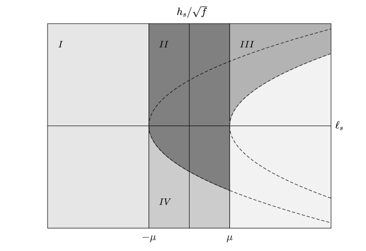
Figure 1: Stark’s problem: the four regions in the $(\ell_{s},h_{s}/\sqrt{f})$ plane.

Table 1: Qualitative description of the trajectories in the $(x,y)$ plane for Stark’s problem. We denote by $i$ the imaginary unit.

Region $I$	$\ell_{s}\in(-\infty,-\mu)$; $h_{s}/\sqrt{f}\in(-\infty,+\infty)$
$V(v)$, $U(u)$ roots	${v}_{1}>0$, ${v}_{2}\in i\mathbb{R}$, ${u}_{1}>0$, ${u}_{2}\in i\mathbb{R}$
$v$, $u$ variable	$v\in[-{v}_{1},{v}_{1}]$, $u\in(-\infty,-{u}_{1}]\cup[{u}_{1},+\infty)$
trajectories type	unbounded, self-intersecting, not encircling the origin
Region $II$	$\ell_{s}\in(-\mu,\mu)$; $h_{s}/\sqrt{f}\in(-\sqrt{2(\mu+\ell_{s})},+\infty)$
$V(v)$, $U(u)$ roots	${v}_{1}>0$, ${v}_{2}\in i\mathbb{R}$, ${u}_{1},{u}_{2}\in\mathbb{C}\setminus\mathbb{R}$
$v$, $u$ variable	$v\in[-{v}_{1},{v}_{1}]$, $u\in(-\infty,+\infty)$
trajectories type	unbounded, self-intersecting, encircling the origin
Region $III$	$\ell_{s}\in(\mu,+\infty)$; $h_{s}/\sqrt{f}\in(\sqrt{-2(\mu-\ell_{s})},+\infty)$
$V(v)$, $U(u)$ roots	${v}_{1}>{v}_{2}>0$, ${u}_{1},{u}_{2}\in\mathbb{C}\setminus\mathbb{R}$
$v$, $u$ variable	$v\in[-{v}_{1},-{v}_{2}]\cup[{v}_{2},{v}_{1}]$, $u\in(-\infty,+\infty)$
trajectories type	unbounded, not self-intersecting
Region $IV$	$\ell_{s}\in(-\mu,\mu)$; $h_{s}/\sqrt{f}\in(-\infty,-\sqrt{2(\mu+\ell_{s})}\,)$
$V(v)$, $U(u)$ roots	${v}_{1}>0$, ${v}_{2}\in i\mathbb{R}$, ${u}_{1}>{u}_{2}>0$
$v$, $u$ variable	$v\in[-{v}_{1},{v}_{1}]$, $u\in(-\infty,-{u}_{1}]\cup[-{u}_{2},{u}_{2}]\cup[{u}_{1},+\infty)$
trajectories type	two types: bounded; unbounded,
	self-intersecting, not encircling the origin

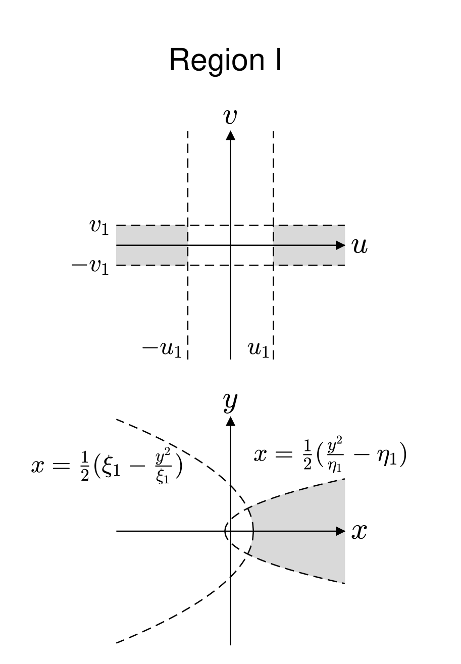
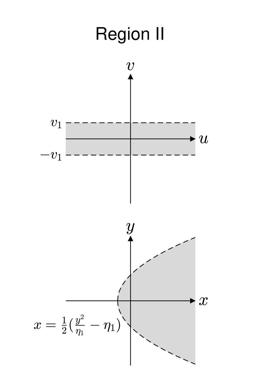
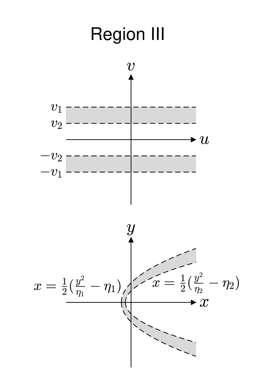
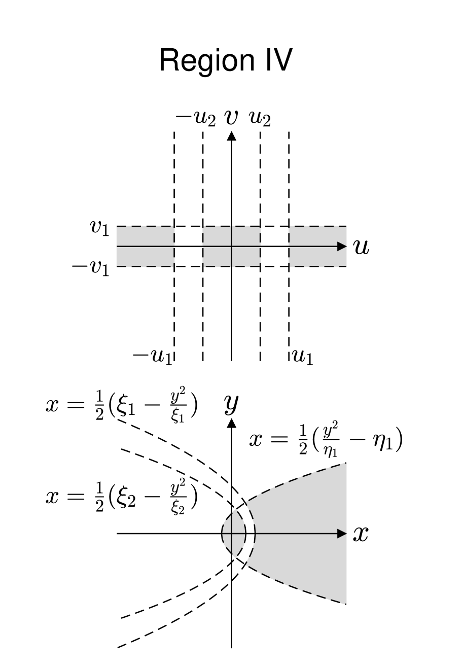
Figure 2: Admissible subsets of the configuration space in $(x,y)$ and $(u,v)$ planes, depending on the region. These subsets are represented by the grey areas; the dashed lines correspond to their boundaries.

Remark 1.

We can have zero velocity points only for some values $\ell_{s},h_{s}$ of the integrals $\mathscr{L}_{s},\mathscr{H}_{s}$. In region $I$ we have the two points

$$(x,y)\in\{(\xi_{1}/2-\eta_{1}/2,\pm\sqrt{\xi_{1}\eta_{1}})\},$$

and in region $IV$ the four points

$$(x,y)\in\{(\xi_{1}/2-\eta_{1}/2,\pm\sqrt{\xi_{1}\eta_{1}}),(\xi_{2}/2-\eta_{1}/2,\pm\sqrt{\xi_{2}\eta_{1}})\}.$$

In regions $II$ and $III$ there cannot be zero velocity points.

Remark 2.

For each region of the $(\ell_{s},h_{s}/\sqrt{f})$ plane, the $v$-component of an orbit is periodic (and bounded). The $u$-component is periodic (and bounded) only if $(\ell_{s},h_{s}/\sqrt{f})$ belongs to region $IV$ and $u^{2}\leq\xi_{2}$. On the contrary, the $u$-component is unbounded if $(\ell_{s},h_{s}/\sqrt{f})$ belongs to one among regions $I$, $II$, $III$, or it belongs to region $IV$, and $u^{2}\geq\xi_{1}$.

Proposition 1.

In case $u(\tau)$ and $v(\tau)$ are periodic solutions of (12), relation

$$\frac{T_{v}}{T_{u}}<1$$ (26)

holds for their periods $T_{u},T_{v}$.

Proof.

The periods $T_{u}$ and $T_{v}$ of the $u$ and $v$ variables can be written as elliptic integrals:

$$T_{u}=\frac{4}{\sqrt{f}}\int_{0}^{\pi/2}\frac{d\varphi}{\sqrt{a_{u}^{2}\cos^{2}\varphi+b_{u}^{2}\sin^{2}\varphi}},\qquad T_{v}=\frac{4}{\sqrt{f}}\int_{0}^{\pi/2}\frac{d\varphi}{\sqrt{a_{v}^{2}\cos^{2}\varphi+b_{v}^{2}\sin^{2}\varphi}},$$

where

$$a_{u}^{2}=\xi_{1}=-\frac{h_{s}}{f}+\sqrt{\frac{h_{s}^{2}}{f^{2}}-\frac{2(\mu+\ell_{s})}{f}},\qquad b_{u}^{2}=\xi_{1}-\xi_{2}=2\sqrt{\frac{h_{s}^{2}}{f^{2}}-\frac{2(\mu+\ell_{s})}{f}},$$

$$a_{v}^{2}=\eta_{1}-\eta_{2}=2\sqrt{\frac{h_{s}^{2}}{f^{2}}+\frac{2(\mu-\ell_{s})}{f}},\qquad b_{v}^{2}=-\eta_{2}=-\frac{h_{s}}{f}+\sqrt{\frac{h_{s}^{2}}{f^{2}}+\frac{2(\mu-\ell_{s})}{f}}.$$

Let $a_{u},b_{u},a_{v},b_{v}$ be the positive square roots of the previous quantities. We note that

$$b_{u}<a_{u}<b_{v}<a_{v}.$$ (27)

Denoting by $M(a,b)$ the arithmetic-geometric mean of two real numbers $a,b$ (see [3]), we have

$$T_{u}=\frac{2\pi}{\sqrt{f}M(a_{u},b_{u})},\qquad T_{v}=\frac{2\pi}{\sqrt{f}M(a_{v},b_{v})}.$$

Since $b_{u}\leq M(a_{u},b_{u})\leq a_{u}$, and $b_{v}\leq M(a_{v},b_{v})\leq a_{v}$, from (27) we obtain

$$M(a_{u},b_{u})<M(a_{v},b_{v}),$$

that corresponds to (26).

∎

3.1 Unstable periodic orbits of brake type

There exists a family of unstable periodic orbits of brake type, ${\bm{x}^{*}}={\bm{x}^{*}}(t;\ell_{s})$, parametrised by $\ell_{s}\in(-\mu,\mu)$.

It is possible to analyse the behaviour of the $u$ and $v$-components of the trajectory in the reduced phase spaces with coordinates $(u,p_{u})$ and $(v,p_{v})$. For this purpose we can take into account the two Hamiltonian dynamics defined by

$$\mathsf{H_{s_{u}}}=\frac{p_{u}^{2}}{2u^{2}}-\frac{2(\mu+\ell_{s})+fu^{4}}{2u^{2}},\qquad\mathsf{H_{s_{v}}}=\frac{p_{v}^{2}}{2v^{2}}-\frac{2(\mu-\ell_{s})-fv^{4}}{2v^{2}},$$

obtained from system (18). $\mathsf{H_{s_{u}}}$ has the two critical points $(p_{u}^{*},\pm u^{*})$, where

$$p_{u}^{*}=0,\qquad u^{*}=\left(\frac{2(\mu+\ell_{s})}{f}\right)^{\frac{1}{4}}.$$

We can show that they are two unstable equilibrium points for the reduced dynamics in the $(u,p_{u})$ plane. In fact, the Jacobian of the Hamiltonian vector field induced by $\mathsf{H_{s_{u}}}$, evaluated in both critical points, is

$$D\mathsf{H_{s_{u}}}=\begin{bmatrix}0&\frac{1}{{\xi^{*}}}\\ 4f&0\\ \end{bmatrix},$$

where

$${\xi^{*}}={u^{*}}^{2}.$$ (28)

At these critical points, the value of $\mathsf{H_{s_{u}}}$ is

$$h_{s}^{*}=-\sqrt{2f(\mu+\ell_{s})},$$ (29)

so that

$${\xi^{*}}=-\frac{h_{s}^{*}}{f}$$ (30)

and $\det D\mathsf{H_{s_{u}}}<0$ at $(p_{u}^{*},\pm u^{*})$.

The level set $\mathsf{H_{s_{v}}}=h_{s}^{*}$ is a closed curve in the $(v,p_{v})$ plane (see Figure 3). Thus, the $v$-component is periodic. This implies that, if $\ell_{s}\in(-\mu,\mu)$ and Stark’s Hamiltonian $\mathscr{H}_{s}$ has the value $h_{s}^{*}$, we have two unstable periodic orbits in the $(u,v)$ plane. They have a constant value of the $u$-component, equal to $\pm u^{*}$, and a constant value of $p_{u}$, equal to zero. Moreover, they are of brake type because each of them develops between two zero velocity points. These are given by $(u^{*},\pm v_{1}^{*})$, with $v_{1}^{*}=v_{1}(h_{s}^{*})$, in one case, and by $(-u^{*},\pm v_{1}^{*})$ in the other. In the $(x,y)$ plane, they correspond to the same periodic orbit $\bm{x}^{*}$, which is a parabolic arc and develops between the zero velocity points $({\xi^{*}}/2-\eta_{1}^{*}/2,\pm\sqrt{{\xi^{*}}\eta_{1}^{*}})$, where $\eta_{1}^{*}=v_{1}^{*2}$. Its trajectory is shown in Figure 4.

The family of brake orbits $\bm{x}^{*}$ exists for values $\ell_{s},h_{s}$ corresponding to the boundary between regions $II$ and $IV$. On this boundary, the values of $\xi_{1}$ and $\xi_{2}$ coincide and are equal to ${\xi^{*}}$.

Remark 3.

For $h_{s}<h_{s}^{*}$ (region $IV$), we have $\xi_{2}<{\xi^{*}}<\xi_{1}$.

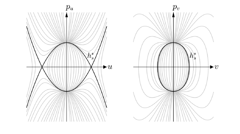
Figure 3: Stark’s problem: phase portraits in the $(p_{u},u)$ and $(p_{v},v)$ planes, for $\ell_{s}=119580$ $\mathrm{k}\mathrm{{}^{3}}\mathrm{m}\mathrm{/}{\mathrm{s}}^{2}$, $f=9.12\times 10^{-9}$ $\mathrm{k}\mathrm{m}\mathrm{/}{\mathrm{s}}^{2}$.

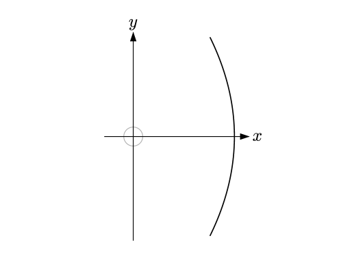
Figure 4: Stark’s problem: unstable periodic orbit of brake type.

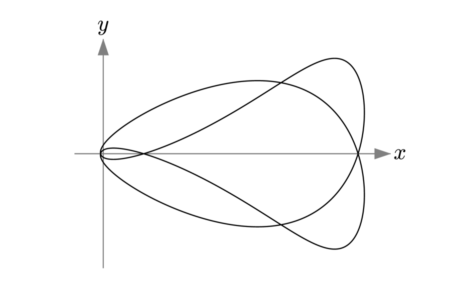
(a) $T_{u}=2T_{v}$

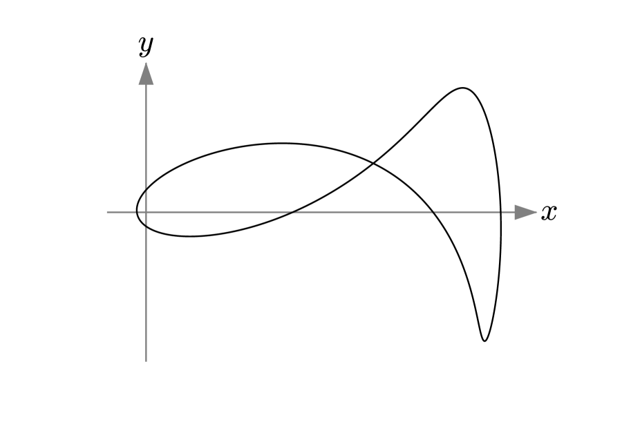
(b) $T_{u}=3T_{v}$

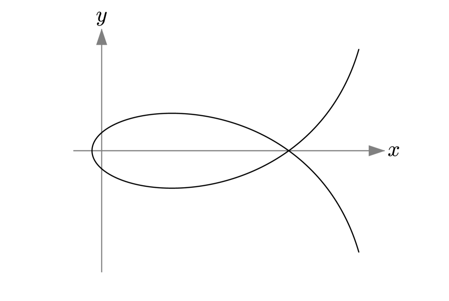
(c) $T_{u}=2T_{v}$

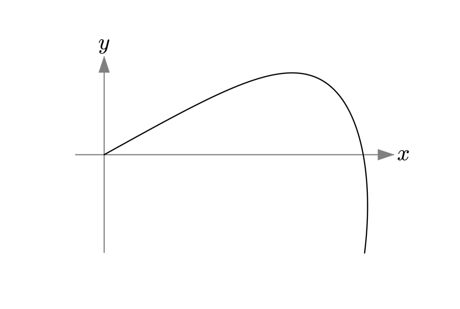
(d) $T_{u}=3T_{v}$

Figure 5: Stark’s problem: some periodic orbits, with $\ell_{s}=348600$ $\mathrm{k}\mathrm{{}^{3}}\mathrm{m}\mathrm{/}{\mathrm{s}}^{2}$, $f=9.12\times 10^{-9}$ $\mathrm{k}\mathrm{m}\mathrm{/}{\mathrm{s}}^{2}$.

3.2 Other periodic orbits

There exists another family of periodic orbits of brake type at the boundary of region $I$, i.e. for $\ell_{s}=-\mu$: they pass through the origin and have a constant value of the $u$-coordinate, equal to zero, in the $(u,v)$ plane, therefore they lie on the $y$ axis in the $(x,y)$ plane. Moreover, there are periodic orbits of brake type in correspondence of $\ell_{s}=\mu$ and $h_{s}<-2\sqrt{f\mu}$. They also pass through the origin and lie on the $y$ axis in the $(x,y)$ plane, but in the $(u,v)$ plane they have a constant value of the $v$-coordinate, equal to zero. If $h_{s}=-2\sqrt{f\mu}$, we obtain the two fixed points $(u,v)=(\pm\sqrt{|h_{s}|/f},0)$ for Stark’s dynamics, corresponding to a single fixed point in the $(x,y)$ plane.
Additional periodic orbits can exist for $(\ell_{s},h_{s}/\sqrt{f})$ belonging to region $IV$, as a consequence of Remark 2. Their peculiarity is that the periods $T_{u}$ and $T_{v}$ are commensurable, that is their quotient $T_{v}/T_{u}$ is rational. In Figure 5 some examples are shown. Note that the orbits in Figures 5(c) and 5(d) are of brake type. In this case, if $T_{u}$ is an odd integer multiple of $T_{v}$, the trajectory passes through the origin as shown in Figure 5(d).

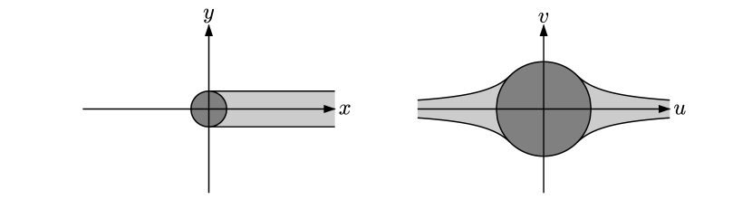
Figure 6: Sun-shadow regions in the $(x,y)$ plane (left), $(u,v)$ plane (right).

4 The Sun-shadow dynamics

The Sun-shadow problem arises by switching dynamics each time the satellite passes through the boundary of the Earth shadow. The flow develops by alternating Kepler’s regime, corresponding to the shadow region, and Stark’s regime, in the out-of-shadow region. As shown in Figure 6, the shadow region is defined as the set $\{(x,y):\ x\geq 0,\ -R\leq y\leq R\}$ in the $(x,y)$ plane. In the $(u,v)$ plane this region has two components: it is the set $\{(u,v):\ -R/u\leq v\leq R/u,\ |u|\geq\sqrt{R}\}$.

At the time $t=0$ of entrance into the shadow, let us consider initial conditions belonging to the set

$$\bigl{\{}(p_{u},p_{v},u,v):\ u>\sqrt{R},\ uv=-R,\ p_{v}u+p_{u}v>0\bigr{\}}.$$ (31)

The last condition is needed to have the velocity vector pointing inside the shadow region. We search for the solutions $(p_{u},p_{v},u,v)$ of the polynomial system

$$\left\{\begin{split}&p_{u}^{2}=2h_{k}u^{2}+2(\mu+\ell_{k})\cr&p_{v}^{2}=2h_{k}v^{2}+2(\mu-\ell_{k})\cr&2c_{k}=p_{v}u-p_{u}v\cr&uv=R\cr\end{split}\right.$$ (32)

with

$$u>\sqrt{R},\qquad v>0,$$

where $c_{k}$ is the value of the angular momentum $\mathscr{C}_{k}$. From system (32), it is possible to obtain the state at the exit point of the shadow region. By eliminating the variables $p_{u},p_{v},v$ we obtain an eight degree polynomial equation in $u$:

$$\begin{split}&(\mu-\ell_{k})^{2}u^{8}-4(\mu-\ell_{k})c_{k}^{2}u^{6}+2\bigl{(}R^{2}(\ell_{k}^{2}-\mu^{2}-4c_{k}^{2}h_{k})+2c_{k}^{4}\bigr{)}u^{4}\cr&-4(\mu+\ell_{k})R^{2}c_{k}^{2}u^{2}+4(\mu+\ell_{k})^{2}R^{4}=0.\cr\end{split}$$ (33)

The roots of (33) come in pairs $\pm u$, which give the same values of $x$. We can select the right value of $x$ using the $y$-component of the Laplace-Lenz integral $\bm{A}_{k}$. Let us call $\bm{U}_{i}=(p_{u_{i}},p_{v_{i}},u_{i},v_{i})^{T}$ the selected solution, corresponding to the state at the entrance point in Stark’s regime. To find the exit point from this regime $\bm{U}_{o}=(p_{u_{o}},p_{v_{o}},u_{o},v_{o})^{T}$, we match the time intervals of $u$ and $v$ to go from $\bm{U}_{i}$ to $\bm{U}_{o}$, that can be computed from equations (19).

In this regime, the angular momentum can change not only in value, but even in sign. Indeed, the satellite can re-enter Kepler’s regime either in the first or third quadrant of the $(u,v)$ plane.

Proposition 2.

Each time the satellite crosses the boundary of the shadow region, we have a leap in energy from $h_{s}$ to $h_{k}$, or vice versa: the variation is equal to $\pm f(\mathrm{bar}{u}^{2}-R^{2}/\mathrm{bar}{u}^{2})/2$, where $\mathrm{bar}{u}$ is the value taken by $u$ at the crossing point. A similar leap occurs from $\ell_{s}$ to $\ell_{k}$, or vice versa. In this case, the variation is equal to $\pm fR^{2}/2$. When the satellite goes back to Stark’s regime, the value of $\mathscr{L}_{s}$ is the same as before crossing the shadow; on the other hand, the energy usually changes unless the orbit is symmetric with respect to the $u$ axis.

Proof.

Assume that the body enters Stark’s regime at the point $(p_{u_{i,1}},p_{v_{i,1}},u_{i,1},v_{i,1})$. Let $h_{s}^{{i,1}}$ be the value of the energy and $\ell_{s}^{\ {i,1}}$ the value of the Laplace-Lenz integral. When the body returns to the shadow region, the integrals vary in the following way:

$$h_{k}^{{o,1}}=h_{s}^{{i,1}}+\frac{f}{2}\biggl{(}u_{o,1}^{2}-\frac{R^{2}}{u_{o,1}^{2}}\biggr{)},$$

$$\ell_{k}^{\ {o,1}}=\ell_{s}^{\ {i,1}}+\frac{f}{2}R^{2},$$

with $u_{o,1}$ the $u$ coordinate of the point on the shadow boundary where the satellite exits from Stark’s regime. When the body enters Stark’s regime again, by passing through the point $(p_{u_{i,2}},p_{u_{i,2}},u_{i,2},v_{i,2})$, similar variations occur:

$$h_{s}^{{i,2}}=h_{k}^{{o,1}}-\frac{f}{2}\biggl{(}u_{i,2}^{2}-\frac{R^{2}}{u_{i,2}^{2}}\biggr{)},$$

$$\ell_{s}^{\ {i,2}}=\ell_{k}^{\ {o,1}}-\frac{f}{2}R^{2}.$$

Thus, we get

$$h_{s}^{{i,2}}=h_{s}^{{i,1}}+\frac{f}{2}\biggl{(}1+\frac{R^{2}}{u_{o,1}^{2}u_{i,2}^{2}}\biggr{)}\bigl{(}u_{o,1}^{2}-u_{i,2}^{2}\bigr{)},$$

$$\ell_{s}^{\ {i,2}}=\ell_{s}^{\ {i,1}},$$

where $h_{s}^{{i,2}}=h_{s}^{{i,1}}$ only if $u_{o,1}=u_{i,2}$. ∎

4.1 Periodic orbits of brake type

We prove the existence of a family of periodic orbits of brake type, $\widehat{\bm{x}}=\widehat{\bm{x}}(t;\ell_{s})$, parametrised by $\ell_{s}$, which are close to the brake periodic orbits $\bm{x}^{*}=\bm{x}^{*}(t;\ell_{s})$ of Stark’s problem, described in Section 3.1. For this purpose, we consider values $\ell_{s}$ in $(-\mu,\mu)$, for which the periodic orbits $\bm{x}^{*}$ exist. In the following we shall restrict the interval $(-\mu,\mu)$ for reasons related to the proof.

The idea of the proof is to search for an initial point $(x,y)=(x_{0},0)$ with $x_{0}>R$, i.e. in Kepler’s regime, allowing to arrive at a zero velocity point $(x_{B},y_{B})$ in Stark’s regime after passing through an exit point $(x_{E},R)$ from the shadow region. We look for an orbit that is symmetric with respect to the $x$ axis, like $\bm{x}^{*}$. Because of the symmetry, $\widehat{\bm{x}}$ oscillates between the points $(x_{B},y_{B})$ and $(x_{B},-y_{B})$. We search for an initial value $x_{0}$ fulfilling

$$x_{0}>{\xi^{*}}/2,$$ (34)

where $({\xi^{*}}/2,0)$ belongs to $\bm{x}^{*}$, see Figure 7(a). The idea behind this choice is that, passing through the shadow, the pushing effect of the solar radiation pressure is lacking. Moreover, we require that $x_{0}$ is such that at the exit point $(x_{E},R)$ the energy fulfils

$$h_{s}<h_{s}^{*},$$ (35)

with $h_{s}^{*}$ given in (29). If $h_{s}>h_{s}^{*}$ we cannot have zero velocity points, see Remark 1.

For the proof, we use the variables $u,v$. The initial point $(x_{0},0)$ corresponds to two possible points $(\pm\sqrt{2x_{0}},0)$ in the $(u,v)$ plane. Similarly, the point $({\xi^{*}}/2,0)$ corresponds to $(\pm\sqrt{{\xi^{*}}},0)$. By symmetry, we can focus only on the $\{u>0\}$ half-plane of the $(u,v)$ plane, see Figure 7(b).

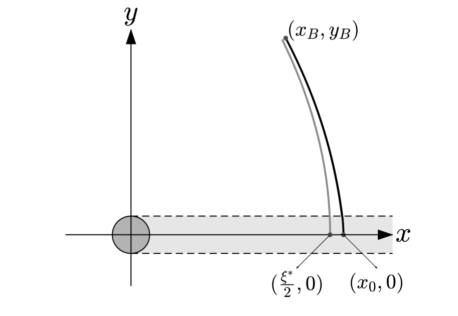
(a) $(x,y)$ plane

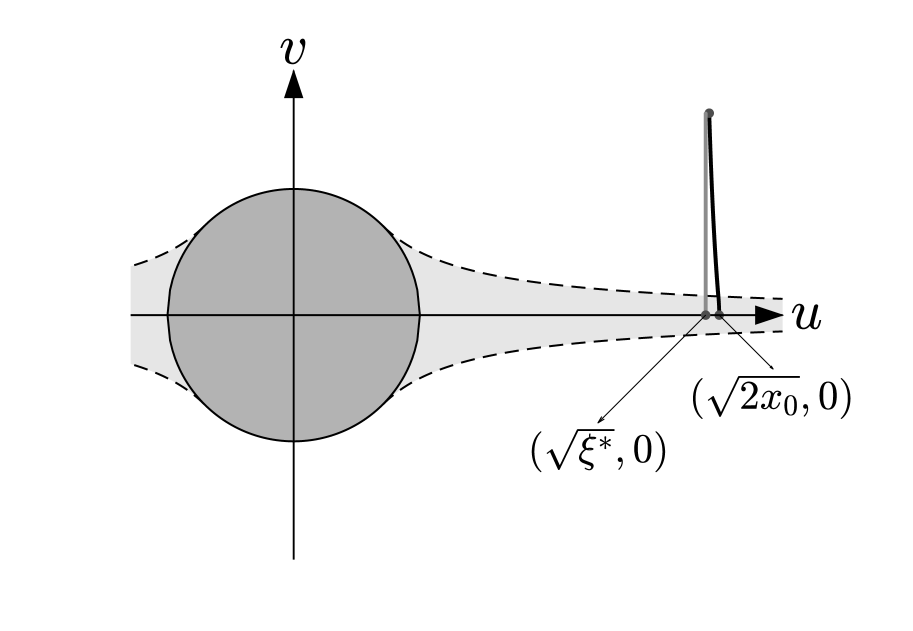
(b) $(u,v)$ plane

Figure 7: A portion of the brake orbit ${\bm{\widehat{x}}}(t;\ell_{s})$ between the horizontal axis and a zero velocity point is represented by the black curve in the $(x,y)$ and $(u,v)$ coordinates. The analogous portion of the brake orbit ${\bm{{x}}}^{*}(t;\ell_{s})$ of Stark’s problem is drawn in grey.

Proposition 3.

If $x_{0}$ is selected so that relations (34), (35) hold, then the exit point $(x_{E},R)$ from the shadow region, with

$$x_{E}=\frac{\xi_{\tiny E}}{2}-\frac{R^{2}}{2\xi_{\tiny E}},$$ (36)

belongs to the unbounded component of the possible configurations corresponding to region IV of Stark’s regime.

Proof.

Because of the symmetry of the orbit with respect to the $x$ axis, in Kepler’s regime the initial state has the form

$$(p_{u},p_{v},u,v)=(0,p_{v_{0}},\sqrt{2x_{0}},0).$$

By system (32) we have

$$p_{v_{0}}=\sqrt{2(\mu-\ell_{k})}$$ (37)

and

$$h_{k}=-\frac{\mu+\ell_{k}}{2x_{0}},$$

where

$$\ell_{k}=\ell_{s}+\frac{f}{2}R^{2}.$$ (38)

Note from relations (37), (38) that we need to restrict the interval of $\ell_{s}$ to $(-\mu,\mu-\frac{f}{2}R^{2})$.

The exit point from the shadow is obtained by solving

$$\left\{\begin{split}&p_{u}^{2}=2h_{k}u^{2}+2(\mu+\ell_{k})\cr&p_{v}^{2}=2h_{k}v^{2}+2(\mu-\ell_{k})\cr&uv=R\cr&p_{u}p_{v}=2uvh_{k},\cr\end{split}\right.$$ (39)

where $p_{v}>0$.

With the last equation we set to zero the $y$-component of the Laplace-Lenz vector, which is a necessary condition for the symmetry with respect to the $x$ axis. There are four possible real solutions of (39), and two of them have positive values of $u$. Between these two, only one corresponds to exiting from the shadow, i.e. fulfils

$$p_{y}=\frac{up_{v}+vp_{u}}{u^{2}+v^{2}}>0.$$

This solution gives the $u$ coordinate at the exit point, whose square is

$$\xi_{\tiny E}=x_{0}+x_{T},$$ (40)

with

$$x_{T}=x_{T}(x_{0})=\sqrt{x_{0}^{2}-a_{k}R^{2}},\qquad a_{k}=\frac{\mu+\ell_{k}}{\mu-\ell_{k}}.$$ (41)

From $\xi_{\tiny E}$, we obtain $x_{E}$ through relation (36), applying the coordinates change (7). Using relation (34), we can write

$$x_{0}={\xi^{*}}/2+\Delta x.$$

We have real values of $\xi_{\tiny E}$ if and only if

$$\Delta x\in\Bigl{(}-\infty,-\frac{{\xi^{*}}}{2}-\sqrt{a_{k}}R\Bigr{]}\cup\Bigl{[}-\frac{{\xi^{*}}}{2}+\sqrt{a_{k}}R,+\infty\Bigr{)}.$$

The last condition is fulfilled for each choice of $\Delta x\geq 0$ if

$$-\frac{{\xi^{*}}}{2}+\sqrt{a_{k}}R\leq 0,$$ (42)

which holds if we further restrict the interval of $\ell_{s}$ to $[{\ell_{s}}^{-},{\ell_{s}}^{+}]$, with

$${\ell_{s}}^{\pm}=-\frac{5}{4}fR^{2}\pm\sqrt{\mu^{2}+\frac{9}{16}f^{2}R^{4}-\frac{5}{2}fR^{2}\mu}.$$

Remark 4.

Since $f\ll 1$, the new range $[{\ell_{s}}^{-},{\ell_{s}}^{+}]$ is slightly smaller than $(-\mu,\mu)$.

The energy in Stark’s regime is

$${\sf h}_{s}(x_{0})=-\frac{\mu+\ell_{k}}{2x_{0}}-\frac{f}{2}\left(x_{0}+x_{T}\right)+\frac{fR^{2}}{2(x_{0}+x_{T})}.$$ (43)

For the proof we need this result:

Lemma 1.

The energy ${\sf h}_{s}$ is a decreasing function of $x_{0}$ in the interval $[\frac{{\xi^{*}}}{2},\infty)$. Moreover, we have

$${\sf h}_{s}({\xi^{*}}/2)>h_{s}^{*}.$$

Proof.

From equation (43), the derivative of ${\sf h}_{s}$ with respect to $x_{0}$ is

$$\frac{d{\sf h}_{s}}{dx_{0}}=\frac{(\mu+\ell_{k})(x_{0}+x_{T})x_{T}-f(x_{0}+x_{T})^{2}x_{0}^{2}-fR^{2}x^{2}_{0}}{2(x_{0}+x_{T})x^{2}_{0}x_{T}}.$$

The denominator is always positive, being $x_{0},x_{T}>0$. We prove that the numerator is negative. Because of relations (29), (30) and (38), this corresponds to showing that

$$(x_{0}+x_{T})\biggl{(}\frac{{{\xi^{*}}}^{2}}{2}x_{T}-(x_{0}+x_{T})x_{0}^{2}\biggr{)}+R^{2}\biggl{(}\frac{1}{2}(x_{0}+x_{T})x_{T}-x_{0}^{2}\biggr{)}<0.$$

This follows from (34) and $x_{0}>x_{T}$. We conclude that $\frac{d{\sf h}_{s}}{dx_{0}}<0$.

Next we prove the second statement of the lemma. We have

$${\sf h}_{s}\left(\frac{{\xi^{*}}}{2}\right)-h_{s}^{*}=-\frac{\mu+\ell_{k}}{{\xi^{*}}}-\frac{f}{4}\Bigl{(}{\xi^{*}}+\sqrt{{\xi^{*}}^{2}-4a_{k}R^{2}}\,\Bigr{)}+\frac{fR^{2}}{{\xi^{*}}+\sqrt{{{\xi^{*}}}^{2}-4a_{k}R^{2}}}-h_{s}^{*}.$$

Using (29), (30), (38) we obtain

$$-\frac{\mu+\ell_{k}}{\xi^{*}}=\frac{h_{s}^{*}}{2}+\frac{f^{2}R^{2}}{2h_{s}^{*}}$$

and we get

$${\sf h}_{s}\left(\frac{{\xi^{*}}}{2}\right)-h_{s}^{*}=\Bigl{(}h_{s}^{*}+\sqrt{{h_{s}^{*}}^{2}-4a_{k}f^{2}R^{2}}\,\Bigr{)}\Biggl{(}-\frac{1}{4}+\frac{f^{2}R^{2}}{2h_{s}^{*}\Bigl{(}-h_{s}^{*}+\sqrt{{h_{s}^{*}}^{2}-4a_{k}f^{2}R^{2}}\,\Bigr{)}}\Biggr{)}.$$

From relation

$$h_{s}^{*}+\sqrt{{h_{s}^{*}}^{2}-4a_{k}f^{2}R^{2}}<0,$$

we conclude that ${\sf h}_{s}({\xi^{*}}/2)-h_{s}^{*}>0$.

∎

Using Lemma 1, we only need to find $x_{0}^{*}>{\xi^{*}}/2$ such that ${\sf h}_{s}(x_{0}^{*})=h_{s}^{*}$ to prove that at the exit time the values of the integrals $(\ell_{s},{\sf h}_{s}(x_{0}))$, with $x_{0}>{\xi^{*}}/2$, belong to region IV. From (29), (30), (38), (41) and (43), solving equation ${\sf h}_{s}(x_{0})=h_{s}^{*}$ corresponds to searching for the roots of

$$g(x_{0})=-4x_{0}^{3}+4{\xi^{*}}x_{0}^{2}+\bigl{(}R^{2}-{\xi^{*}}^{2}+2a_{k}R^{2}\bigr{)}x_{0}-\bigl{(}(2x_{0}-{\xi^{*}})^{2}+R^{2}\bigr{)}x_{T}.$$

From relations (34) and (41), it holds

$$Cx_{0}<x_{T}<x_{0},\qquad C=\sqrt{1-4a_{k}\frac{R^{2}}{{\xi^{*}}^{2}}}.$$ (44)

Thus, we have

$$g_{-}(x_{0})\leq g(x_{0})\leq g_{+}(x_{0}),$$

where

$$\begin{split}&g_{-}(x_{0})=-2x_{0}\bigl{(}4x_{0}^{2}-4{\xi^{*}}x_{0}+{\xi^{*}}^{2}-a_{k}R^{2}\bigr{)},\cr&g_{+}(x_{0})=-(1+C)x_{0}\left(4x_{0}^{2}-4{\xi^{*}}x_{0}+{\xi^{*}}^{2}-\frac{1-C}{1+C}R^{2}-\frac{2}{1+C}a_{k}R^{2}\right).\cr\end{split}$$

The polynomials $g_{+}$ and $g_{-}$ have three roots, but only one is larger than ${\xi^{*}}/2$. Denoting the latter with $x_{0}^{+}$ and $x_{0}^{-}$ respectively, we get

$$x_{0}^{-}=\frac{{\xi^{*}}}{2}+C_{1},\qquad x_{0}^{+}=\frac{{\xi^{*}}+C_{2}}{2},$$

with

$$C_{1}=\frac{R}{2}\sqrt{a_{k}},\qquad C_{2}=R\,\sqrt{\frac{1-C+2a_{k}}{1+C}}.$$

This shows the existence of $x_{0}^{*}>\xi^{*}/2$, solution of ${\sf h}_{s}(x_{0})=h_{s}^{*}$.

Next we show that the exit point belongs to the unbounded component of the configuration set, i.e. that $\xi_{E}>\xi_{1}$ holds for each $x_{0}>x_{0}^{*}$. Since $x_{0}^{-}<x_{0}^{*}<x_{0}^{+}$ and $\xi_{\tiny E}$, given in (40), is an increasing function of $x_{0}$, we have

$$\xi_{\tiny E}(x_{0}^{-})<\xi_{\tiny E}(x_{0}^{*})<\xi_{\tiny E}(x_{0}^{+})$$ (45)

where

$$\begin{split}&\xi_{\tiny E}(x_{0}^{-})=\frac{{\xi^{*}}}{2}+C_{1}+\sqrt{\left(\frac{{\xi^{*}}}{2}+C_{1}\right)^{2}-a_{k}R^{2}},\cr&\xi_{\tiny E}(x_{0}^{+})=\frac{{\xi^{*}}+C_{2}}{2}+\sqrt{\frac{\left({\xi^{*}}+C_{2}\right)^{2}}{4}-a_{k}R^{2}}.\cr\end{split}$$

Relation (42) implies $\xi_{\tiny E}(x_{0}^{-})>{\xi^{*}}$. Thus $\xi_{\tiny E}(x_{0}^{*})>{\xi^{*}}$. Since in region IV we have $\xi_{2}<{\xi^{*}}<\xi_{1}$, and $\xi_{\tiny E}<\xi_{2}$ or $\xi_{\tiny E}>\xi_{1}$, the latter relation holds.

∎

Remark 5.

Proposition 3 yields

$$2x_{0}>\xi_{\tiny E}>\xi_{1}>{\xi^{*}}>\xi_{2}>0,$$

and

$${\xi^{*}}+C_{1}<\xi_{\tiny E}^{*}<{\xi^{*}}+C_{2},$$

where $\xi_{\tiny E}^{*}=\xi_{\tiny E}(x_{0}^{*})$.

To search for a zero velocity point $(x_{B},y_{B})$ we use the coordinates $u,v$ and the fictitious time $\tau$. The maps $u(\tau)$, $v(\tau)$ become stationary at $\tau=\tau_{u},\tau_{v}$ respectively, where

$$\tau_{u} =\int_{u_{1}}^{\sqrt{\xi_{\tiny E}}}\frac{du}{\sqrt{fu^{4}+2h_{s}u^{2}+2(\mu+\ell_{s})}},$$

$$\tau_{v} =\int_{\frac{R}{\sqrt{\xi_{\tiny E}}}}^{v_{1}}\frac{dv}{\sqrt{-fv^{4}+2h_{s}v^{2}+2(\mu-\ell_{s})}}.$$

We search for value of $x_{0}$ such that

$$\tau_{u}=\tau_{v},$$ (46)

which corresponds to reach a zero velocity point.

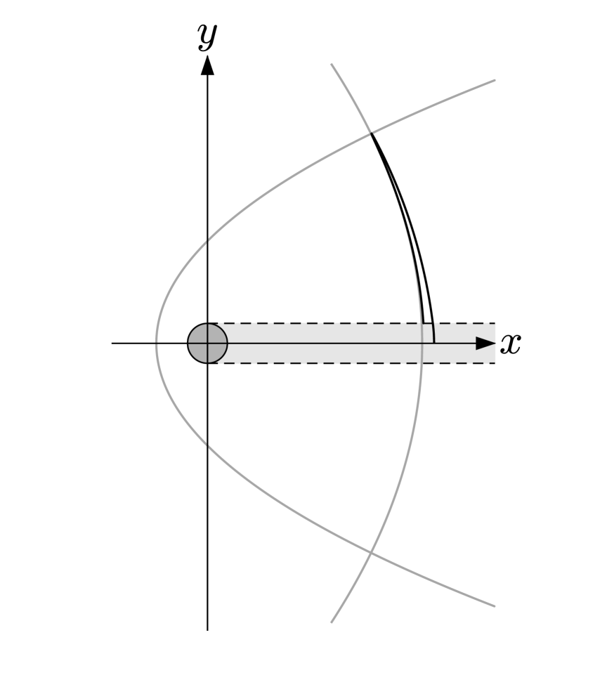
(a) $\tau_{u}<\tau_{v}$

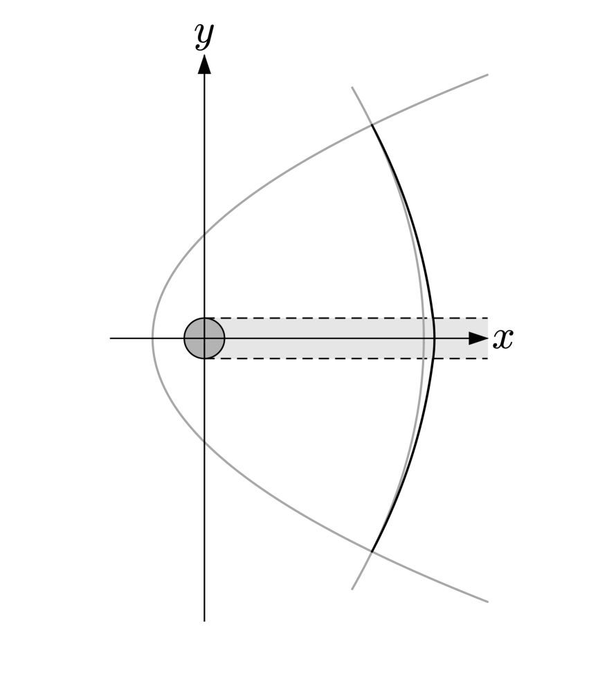
(b) $\tau_{u}=\tau_{v}$

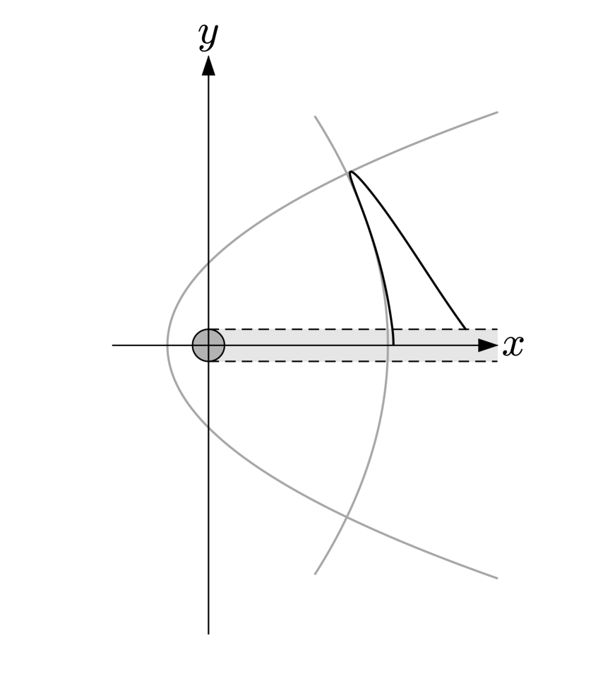
(c) $\tau_{u}>\tau_{v}$

Figure 8: Brake orbit (a) and two close trajectories (b) and (c). The grey arcs of parabola represent the boundaries defining the unbounded admissible subset of the configuration space in Stark’s regime (see Figure 2 for a comparison).

From now on, we use $h_{s}\in J=(-\infty,h_{s}^{*})$ as independent variable, in place of $x_{0}$. Following [1] we can write the integrals $\tau_{u},\tau_{v}$ as

$$\tau_{u}(h_{s}) =\frac{1}{\sqrt{f\xi_{1}}}\int_{0}^{\arcsin r_{\xi}}\frac{d\varphi}{\sqrt{1-\frac{\xi_{2}}{\xi_{1}}\sin^{2}\varphi}},$$ (47)

$$\tau_{v}(h_{s}) =\frac{1}{\sqrt{f\Delta\eta}}\int_{0}^{\arcsin\sqrt{1-\frac{R^{2}}{\xi_{\tiny E}\eta_{1}}}}\frac{d\varphi}{\sqrt{1-\frac{\eta_{1}}{\Delta\eta}\sin^{2}\varphi}},$$ (48)

where

$$r_{\xi}=\sqrt{\frac{\xi_{\tiny E}-\xi_{1}}{\xi_{\tiny E}-\xi_{2}}},\qquad\Delta\eta=\eta_{1}-\eta_{2}.$$

We use the result proved below.

Lemma 2.

The following properties hold:

• $\tau_{u}$ is a strictly increasing function of $h_{s}$ and

  $$\lim_{h_{s}\to h_{s}^{*}}\tau_{u}=+\infty,$$ (49)

• $\tau_{v}$ is not monotone in $h_{s}$ and

  $$\limsup_{h_{s}\to h_{s}^{*}}\tau_{v}<+\infty.$$ (50)

Proof.

i) The derivative of $\tau_{u}$ with respect to $h_{s}$ can be written as

$$\frac{d\tau_{u}}{dh_{s}}=\frac{1}{\sqrt{f\xi_{1}}}\frac{1}{\Delta\xi}\left(\frac{1}{f}\int_{0}^{\arcsin r_{\xi}}\frac{1+\frac{\xi_{2}}{\xi_{1}}\sin^{2}\varphi}{\left(1-\frac{\xi_{2}}{\xi_{1}}\sin^{2}\varphi\right)^{\frac{3}{2}}}d\varphi+\frac{1}{2}\sqrt{\frac{\xi_{1}}{\xi_{\tiny E}}}\frac{\xi_{\tiny E}-\xi_{2}}{r_{\xi}}\ \frac{dr_{\xi}^{2}}{dh_{s}}\right),$$

where

$$\Delta\xi=\xi_{1}-\xi_{2}.$$

Therefore, to prove that $\tau_{u}$ is strictly increasing, it is sufficient to show that

$$\frac{dr_{\xi}^{2}}{dh_{s}}=\frac{d}{dh_{s}}\left(\frac{\xi_{\tiny E}-\xi_{1}}{\xi_{\tiny E}-\xi_{2}}\right)>0.$$ (51)

From relations

$$\begin{split}&\frac{d\xi_{1}}{dh_{s}}=-\frac{2\xi_{1}}{f\Delta\xi}<0,\qquad\frac{d\xi_{2}}{dh_{s}}=\frac{2\xi_{2}}{f\Delta\xi}>0,\cr&\frac{d\xi_{\tiny E}}{dh_{s}}=\frac{\xi_{\tiny E}}{\frac{(\mu+\ell_{k})x_{T}}{2x_{0}^{2}}-\frac{f}{2}\xi_{\tiny E}-\frac{f}{2}\frac{R^{2}}{\xi_{\tiny E}}}<0,\cr\end{split}$$

where the latter follows from (28), (38), (40) and $x_{0}>x_{T}$, we see that

$$\frac{d(\xi_{\tiny E}-\xi_{2})}{dh_{s}}<0.$$

Moreover, we have

$$\frac{d(\xi_{\tiny E}-\xi_{1})}{dh_{s}}>0,$$ (52)

in fact, relations (28), (38) and (40) yield that (52) is equivalent to

$$R^{2}\xi_{1}\left(\frac{1}{x_{0}+x_{T}}-\frac{x_{T}}{2x_{0}^{2}}\right)+\xi_{\tiny E}\xi_{2}-\xi_{1}\frac{{{\xi^{*}}}^{2}}{2x_{0}^{2}}x_{T}>0.$$

which follows from $x_{0}>x_{T}$, $\xi_{2}={\xi^{*}}^{2}/\xi_{1}$ (see (24) and (28)), and Remark 5. This proves (51).

Furthermore, we have

$$\lim_{h_{s}\to h_{s}^{*}}\xi_{1}=\lim_{h_{s}\to h_{s}^{*}}\xi_{2}={\xi^{*}}$$

and (30) holds, so that

$$\lim_{h_{s}\to h_{s}^{*}}\tau_{u}=\frac{1}{\sqrt{f{\xi^{*}}}}\int_{0}^{\frac{\pi}{2}}\frac{d\varphi}{\sqrt{1-\sin^{2}\varphi}}=+\infty.$$

This concludes the proof of i).

ii) We have

$$\tau_{v}<\frac{1}{\sqrt{f\Delta\eta}}\int_{0}^{\pi/2}\frac{d\varphi}{\sqrt{1-\frac{\eta_{1}}{\Delta\eta}\sin^{2}\varphi}}=\frac{1}{\sqrt{f\Delta\eta}}\frac{\pi}{2M\Bigl{(}1,\sqrt{1-\frac{\eta_{1}}{\Delta\eta}}\Bigr{)}},$$

so that

$$\limsup_{h_{s}\to h_{s}^{*}}\tau_{v}\leq\frac{\pi}{2\sqrt[4]{\mu f}}\frac{1}{2\sqrt{1-\frac{-{\xi^{*}}+2\sqrt{\mu/f}}{4\sqrt{\mu/f}}}}<+\infty.$$

∎

Using the previous result, to show that a solution of (46) exists, we only need to find a value of the energy $h_{s}\in J$ such that

$$\tau_{u}(h_{s})<\tau_{v}(h_{s}).$$

Lemma 3.

There exists $\mathrm{bar}{h}_{s}\in J$ and two functions $\tilde{\tau}_{u}(h_{s}),\tilde{\tau}_{v}(h_{s})$ such that

$$\tau_{v}(\mathrm{bar}{h}_{s})>\tilde{\tau}_{v}(\mathrm{bar}{h}_{s})=\tilde{\tau}_{u}(\mathrm{bar}{h}_{s})>\tau_{u}(\mathrm{bar}{h}_{s}).$$

Proof.

Using relation

$$\sqrt{1-\frac{\eta_{1}}{\Delta\eta}\sin^{2}\varphi}<1$$

we get

$$\tau_{v}>\frac{1}{\sqrt{f\Delta\eta}}\arcsin\sqrt{1-\frac{R^{2}}{\xi_{\tiny E}\eta_{1}}}$$

in the interval $J$, where the function $\xi_{\tiny E}\eta_{1}$ is decreasing. Indeed, we have

$$\frac{d(\xi_{\tiny E}\eta_{1})}{dh_{s}}=\frac{\xi_{\tiny E}\eta_{1}}{f}\Biggl{(}\frac{1}{\sqrt{\frac{h_{s}^{2}}{f^{2}}+\frac{2(\mu-\ell_{s})}{f}}}-\frac{1}{\frac{\xi_{\tiny E}}{2}+\frac{R^{2}}{2\xi_{\tiny E}}-\frac{(\mu+\ell_{k})x_{T}}{2fx_{0}^{2}}}\Biggr{)}<0$$

which follows from (43), $x_{0}>x_{T}$ and $\ell_{s}\in[\ell_{s}^{-},\ell_{s}^{+}]$. Thus

$$\xi_{\tiny E}\eta_{1}>\xi_{\tiny E}^{*}\eta_{1}^{*},\qquad\eta_{1}^{*}=\eta_{1}(h_{s}^{*})=-{\xi^{*}}+2\sqrt{\mu/f}.$$

Since $\xi_{\tiny E}^{*}>{\xi^{*}}$ (see Remark 5), we obtain

$$\frac{1}{\sqrt{f\Delta\eta}}\arcsin\sqrt{1-\frac{R^{2}}{\xi_{\tiny E}\eta_{1}}}>\frac{1}{\sqrt{f\Delta\eta}}\arcsin\sqrt{1-\frac{R^{2}}{{\xi^{*}}\eta_{1}^{*}}}.$$

Moreover, we have

$$\left(\frac{\Delta\eta}{2}\right)^{\frac{1}{2}}=\left(\frac{h_{s}^{2}}{f^{2}}+2\frac{\mu-\ell_{s}}{f}\right)^{1/4}<\left(\xi_{1}^{2}+2\frac{\mu-\ell_{s}}{f}\right)^{1/4}<\left(\xi_{1}+\sqrt{\frac{2(\mu-\ell_{s})}{f}}\right)^{1/2}.$$

Hence, we can set

$$\tilde{\tau}_{v}(h_{s})=\frac{1}{\sqrt{2f}\left(\xi_{1}+\sqrt{\frac{2(\mu-\ell_{s})}{f}}\right)^{1/2}}\arcsin\sqrt{1-\frac{R^{2}}{{\xi^{*}}\eta_{1}^{*}}}.$$

Then, using

$$\sqrt{1-\frac{\xi_{2}}{\xi_{1}}\sin^{2}{\phi}}>\cos{\phi},$$

we get

$$\begin{split}&\tau_{u}<\frac{1}{2}\frac{1}{\sqrt{f\xi_{1}}}\log\left(1+\frac{2r_{\xi}}{1-r_{\xi}}\right)<\frac{1}{\sqrt{f\xi_{1}}}\left(\frac{r_{\xi}}{1-r_{\xi}}\right)\cr&=\frac{1}{\sqrt{f\xi_{1}}}\left(\frac{1}{\sqrt{1+\frac{\Delta\xi}{\xi_{\tiny E}-\xi_{1}}}-1}\right)<\frac{1}{\sqrt{f\xi_{1}}}\left(\frac{1}{\sqrt{1+\frac{\Delta\xi}{C_{2}}}-1}\right)\cr\end{split}$$

which follows from $0<r_{\xi}<1$ for $h_{s}\in J$ and Remark 5. From relation

$$\left(1+\frac{1}{\xi_{1}}\sqrt{\frac{2(\mu-\ell_{s})}{f}}\right)^{1/2}<\left(1+\frac{1}{{\xi^{*}}}\sqrt{\frac{2(\mu-\ell_{s})}{f}}\right)^{1/2}$$

we have

$$\tilde{\tau}_{u}(h_{s})=\frac{1}{\sqrt{f}}\frac{\left(1+\frac{1}{{\xi^{*}}}\sqrt{\frac{2(\mu-\ell_{s})}{f}}\right)^{1/2}}{\left(\xi_{1}+\sqrt{\frac{2(\mu-\ell_{s})}{f}}\right)^{1/2}}\frac{1}{\sqrt{1+\frac{\Delta\xi}{C_{2}}}-1}.$$

Set

$$K_{1}=\sqrt{2}\left(1+\frac{1}{{\xi^{*}}}\sqrt{\frac{2(\mu-\ell_{s})}{f}}\right)^{1/2},\qquad K_{2}=\arcsin\sqrt{1-\frac{R^{2}}{{\xi^{*}}\eta_{1}^{*}}}.$$

We obtain $\tilde{\tau}_{u}=\tilde{\tau}_{v}$ in

$$\mathrm{bar}{h}_{s}=-f\left({\xi^{*}}^{2}+\frac{C_{2}^{2}}{4}\frac{K_{1}^{2}}{K_{2}^{2}}\left(2+\frac{K_{1}}{K_{2}}\right)^{2}\right)^{1/2}.$$ (53)

∎

This concludes the proof of the existence of a family of brake periodic orbits $\widehat{\bm{x}}(t;\ell_{s})$ parametrised by $\ell_{s}$.

5 The Sun-shadow map

To study the Sun-shadow dynamics, it is useful to construct a Poincaré-like map. Traditionally, the Poincaré maps of autonomous two-dimensional Hamiltonian systems are defined by fixing the value of the Hamiltonian. This is not possible for the Sun-shadow dynamics, since the Hamiltonian is not conserved along the flow, see Proposition 2. However, here we can fix the value of $\mathscr{L}_{s}$. Indeed, even though $\mathscr{L}_{s}$ is not a constant of motion as well, it assumes the same value in Stark’s regime before and after the satellite crosses the shadow. To define a Poincaré map we also need to introduce a section. The selected section corresponds to the upper boundary of the shadow region in the $(x,y)$ configuration space, i.e. to $y=R$, $x\geq 0$. We consider trajectories leaving the section with $p_{y}>0$, in the outward direction with respect to the shadow region. Since the dependence on the coordinates is decoupled in the variables $u,v$ (see (17), (18)), we decided to use them to define the map. Thus, we define the Sun-shadow map as

$$\begin{split}\mathfrak{S}:{\cal D}\subset\mathbb{R}^{2}&\to\mathbb{R}^{2},\cr(u,p_{u})&\mapsto(u^{\prime},p^{\prime}_{u}),\cr\end{split}$$

where the domain ${\cal D}$ is discussed below, and $(u,p_{u}),(u^{\prime},p^{\prime}_{u})$ belong to the section $\Sigma$ defined as

$$\Sigma=\{(p_{u},p_{v},u,v):\ |u|\geq\sqrt{R},\ uv=R,\ up_{v}>\max(0,-p_{u}v),\ \mathscr{L}_{s}=\ell_{s}\}.$$

The conditions $|u|\geq\sqrt{R}$, $uv=R$ are necessary to select the desired section in the $(x,y)$ configuration space. The condition $up_{v}>-p_{u}v$ is equivalent to $p_{y}>0$ (see (8)). The additional condition, $up_{v}>0$, assures that every point $(u,p_{u})\in\Sigma$ corresponds to only one trajectory. Indeed, there are points $(u,p_{u})$ for which $p_{y}>0$ in both the cases $p_{v}>0$ and $p_{v}<0$.

Proposition 4.

The map $\mathfrak{S}$ is not defined in the points $(u,p_{u})$ with

$$p^{2}_{u}\leq 2(\mu+\ell_{s})+fR^{2}+(f-2(\mu-\ell_{s})/R^{2})u^{4}.$$ (54)

Moreover, in the second and fourth quadrant of the $(u,p_{u})$ plane $\mathfrak{S}$ is not defined if $\ell_{s}>\mu-\frac{fR^{2}}{2}$, while if $\ell_{s}<\mu-\frac{fR^{2}}{2}$ it is not defined only in the points $(u,p_{u})$ with

$$u^{4}\leq\frac{2(\mu+\ell_{s})+fR^{2}}{2(\mu-\ell_{s})-fR^{2}}R^{2}.$$ (55)

Proof.

For each point $(u,p_{u})$ in the domain of the map, we have

$$v=\frac{R}{u},$$

and $p_{v}$ is defined by (18)₂. Condition (54) corresponds to $p_{v}^{2}\leq 0$, that is not possible. In the second and fourth quadrant of the $(u,p_{u})$ plane, the condition $up_{v}>\max(0,-p_{u}v)$ results in

$$p_{v}u>-p_{u}\frac{R}{u}$$

which implies

$$\bigl{(}2(\mu-\ell_{s})-fR^{2}\bigr{)}u^{4}-2(\mu+\ell_{s})-fR^{4}>0.$$

If $\ell_{s}>\mu-\frac{fR^{2}}{2}$, we get

$$u^{4}<\frac{2(\mu+\ell_{s})+fR^{2}}{2(\mu-\ell_{s})-fR^{2}}R^{2}<0,$$

meaning that the map is not defined. On the other hand, if $\ell_{s}<\mu-\frac{fR^{2}}{2}$, the previous condition is fulfilled for

$$u^{4}>\frac{2(\mu+\ell_{s})+fR^{2}}{2(\mu-\ell_{s})-fR^{2}}R^{2}.$$

∎

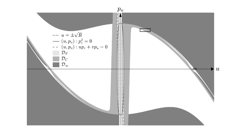
Figure 9: The domain ${{\cal D}}$ of the Sun-shadow map is represented by the white area. $\mathrm{k}\mathrm{{}^{3}}\mathrm{m}\mathrm{/}{\mathrm{s}}^{2}$, $f=9.12\times 10^{-9}$ $\mathrm{k}\mathrm{m}\mathrm{/}{\mathrm{s}}^{2}$. A magnification of the region in the small and smaller rectangles is shown in Figures 11 and 12 respectively.

The domain ${\cal D}\subset\mathbb{R}^{2}$ does not include the points defined in Proposition 55, nor the points corresponding to trajectories which go to infinity or collide with the Earth before going back to $\Sigma$. In Figure 9, for a specific choice of $\ell_{s}$ and $f$, the domain ${{\cal D}}$ is drawn as the white area in a portion of the $(u,p_{u})$ plane. The light grey region represents the set ${\cal D}_{F}$ of forbidden points in Proposition 55. The other two grey areas contain part of the sets ${\cal D}_{\infty}$ (darker) and ${\cal D}_{C}$ (lighter) corresponding to the trajectories which go to infinity and collide with the Earth, respectively.

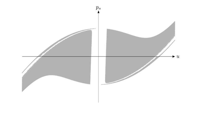
Figure 10: The image of the Sun-shadow map.

Figure 10 shows the image of the domain ${\cal D}$ under $\mathfrak{S}$ in the same portion of the $(u,p_{u})$ plane represented in Figure 9.

Remark 6.

In the image of the map we may have points belonging to ${\cal{D}}_{\infty}$ or ${\cal{D}}_{C}$, so that we cannot iterate the map again.

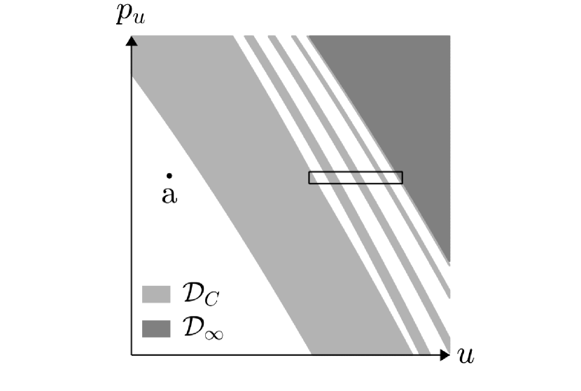
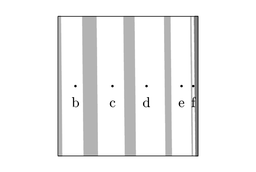
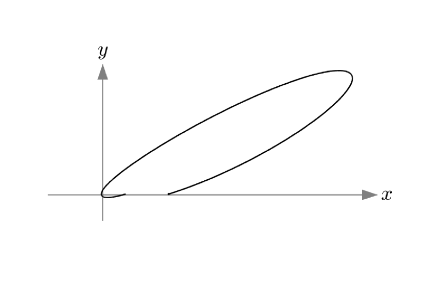
(a)

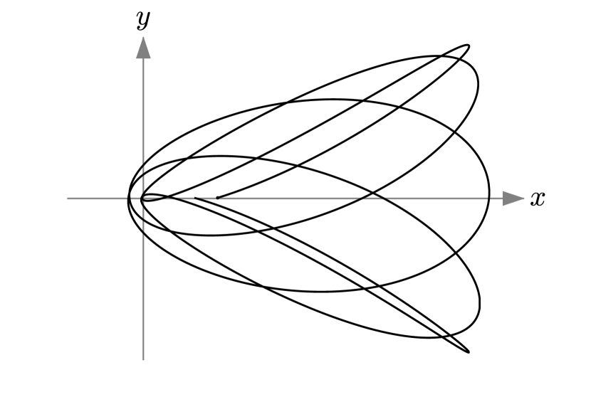
(b)

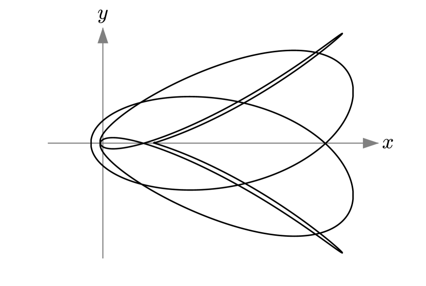
(c)

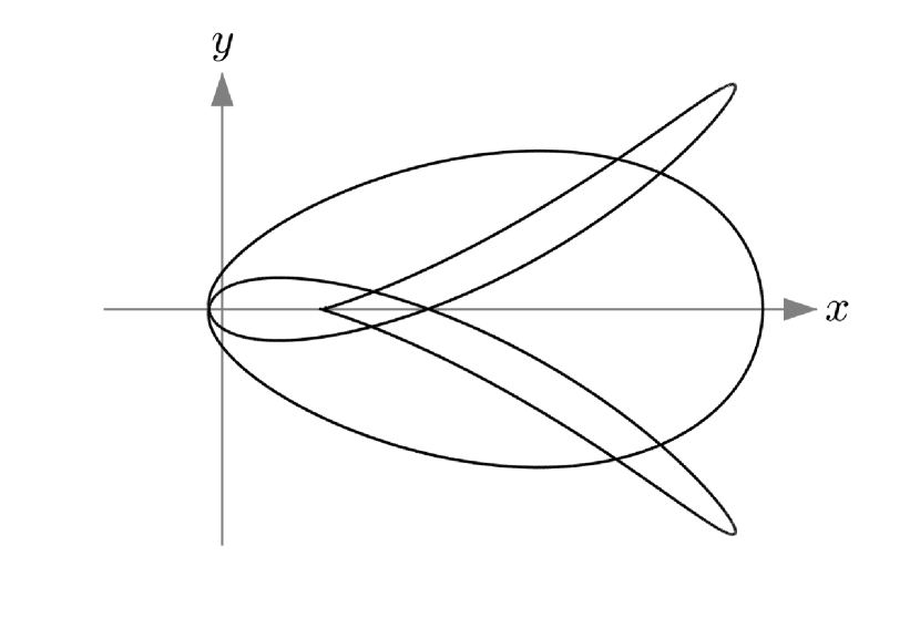
(d)

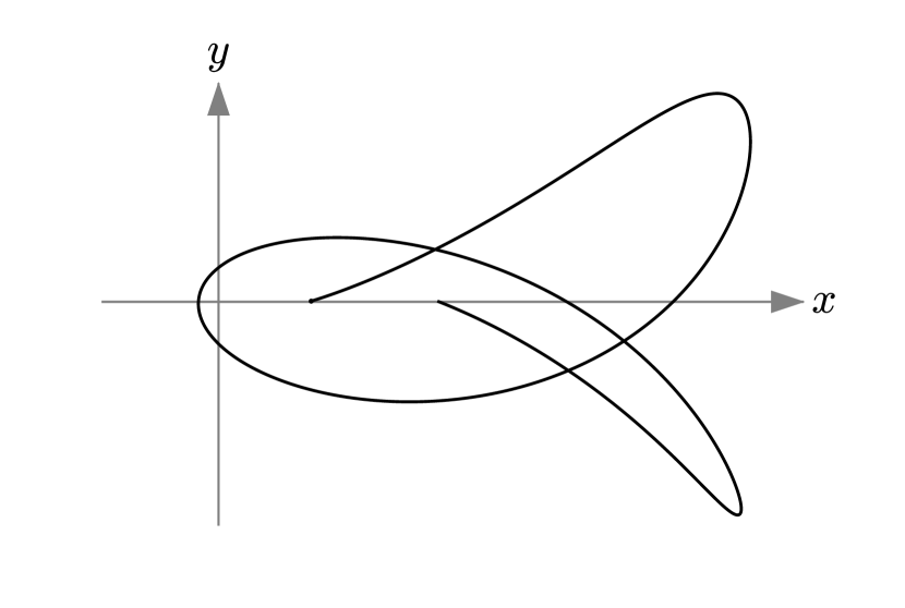
(e)

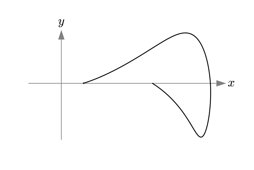
(f)

Figure 11: Orbits with different winding numbers, corresponding to one iteration of $\mathfrak{S}$. The selected initial points are shown in the two top pictures and are labeled with a, b, c, d, e, f. On top right there is the magnification of the small rectangular region on top left.

In Figure 11, the magnification of the larger rectangular region appearing in Figure 9 highlights the complexity of the structure of ${{\cal D}}$. We have selected five points, labelled with b, c, d, e, f, in the white ‘corridors’, and one point, labelled with a, in the larger white region on the left. In the same figure we show the portion of the trajectories corresponding to one iteration of the selected points under the map. A winding number around the origin can be associated to each trajectory by joining with a straight line their initial and final points. The values of this topological invariant are $-4$, $-3$, $-2$, $-1$, $0$, $+1$ for the cases (b), (c), (d), (e), (f), (a), respectively. Since we get a different value for all these cases, the white corridors must belong to different connected components of ${\cal D}$.

Proposition 5.

The map $\mathfrak{S}$ is differentiable in its definition domain ${\cal D}$.

Proof.

Let $\bm{\Phi}_{s}(\tau;{\bm{U}},\tau_{0})$ and $\bm{\Phi}_{k}(\tau;{\bm{U}},\tau_{0})$ be the integral flow of Stark’s and Kepler’s dynamical systems (11), (12). Consider $(u,p_{u})\in{\cal D}$ and the corresponding orbit in the Sun-shadow dynamics. Before it goes back to the section $\Sigma$, the dynamical regime will change $n$ times, with $n$ depending on the shape of the trajectory. The first regime will be always Stark’s, the last will be Kepler’s. Let us introduce a finite sequence of sections $\Sigma_{i}$, $i=0,\ldots,n$ where the dynamics changes, with $\Sigma_{0}=\Sigma_{n}=\Sigma$. Each of them is given by $s_{i}({\bm{U}})=0$: for the section $\Sigma$ we have $s_{i}=uv-R$, while for the intermediate sections, with $i=1,\ldots,n-1$, we have $s_{i}=uv+R$ or $s_{i}=uv-R$ depending on the boundary of the shadow region that is crossed when the dynamics changes. It is possible to define the maps $\mathfrak{S}_{i}$

$$\begin{split}\mathfrak{S}_{i}:{\cal D}_{i}\subset\mathbb{R}^{2}&\to\mathbb{R}^{2},\cr(u^{i},p^{i}_{u})&\mapsto(u^{i+1},p^{i+1}_{u}),\cr\end{split}$$ (56)

where ${\cal D}_{i}$ is made of the points

$${\bm{U}}^{i}=(p^{i}_{u},p^{i}_{v},u^{i},v^{i})^{T}\in\Sigma_{i},\qquad v^{i}=\pm R/u^{i},\qquad p^{i}_{v}=p_{v}(p^{i}_{u},u^{i}).$$

The Sun-shadow map will be given by

$$\mathfrak{S}=\mathfrak{S}_{n-1}\circ...\mathfrak{S}_{2}\circ\mathfrak{S}_{1}\circ\mathfrak{S}_{0}.$$

Thus, we have

$$D\mathfrak{S}(u,p_{u})=\frac{\partial(u^{\prime},p^{\prime}_{u})}{\partial(u,p_{u})}=\frac{\partial(u^{\prime},p^{\prime}_{u})}{\partial(u^{n-1},p^{n-1}_{u})}\frac{\partial(u^{n-1},p^{n-1}_{u})}{\partial(u^{n-2},p^{n-2}_{u})}...\frac{\partial(u^{2},p^{2}_{u})}{\partial(u^{1},p^{1}_{u})}\frac{\partial(u^{1},p^{1}_{u})}{\partial(u,p_{u})}$$ (57)

where

$$\frac{\partial(u^{i+1},p^{i+1}_{u})}{\partial(u^{i},p^{i}_{u})}=A\Big{(}\bm{X}_{i+1}({\bm{U}}_{i+1})\frac{\partial\tau}{\partial{\bm{U}}_{i}}+\frac{\partial\bm{\Phi}_{i+1}}{\partial{\bm{U}}_{i}}(\tau({\bm{U}}_{i}),{\bm{U}}_{i},\tau_{i})\Big{)}\frac{\partial{\bm{U}}_{i}}{\partial(u^{i},p^{i}_{u})},$$

with

$$A=\begin{bmatrix}1&0&0&0\\ 0&0&1&0\end{bmatrix}.$$

The integral flow $\bm{\Phi}_{i+1}$ (resp. $\bm{X}_{i+1}$) is equal to either $\bm{\Phi}_{s}$ or $\bm{\Phi}_{k}$ (resp. $\bm{X}_{s}$ or $\bm{X}_{k}$) depending on the regime between the two sections. The term $\partial\tau/\partial{\bm{U}}_{i}$ can be computed as

$$\frac{\partial\tau}{\partial{\bm{U}}_{i}}=-\frac{1}{\frac{\partial s_{i+1}}{\partial{\bm{U}}}({\bm{U}}_{i+1})\cdot\bm{X}_{i+1}({\bm{U}}_{i+1})}\Big{(}\frac{\partial s_{i+1}}{\partial{\bm{U}}}({\bm{U}}_{i+1})\Big{)}^{T}\ \frac{\partial\bm{\Phi}_{i+1}}{\partial{\bm{U}}_{i}}(\tau({\bm{U}}_{i}),{\bm{U}}_{i},\tau_{i}),$$

see [15], while $\partial\bm{\Phi}_{i+1}/\partial{\bm{U}}_{i}$ fulfils

$$\begin{split}&\frac{d}{d\tau}\Big{(}\frac{\partial\bm{\Phi}_{i+1}}{\partial\bm{U}_{i}}(\tau({\bm{U}}_{i}),{\bm{U}}_{i},\tau_{i})\Big{)}=\frac{\partial\bm{X}_{i+1}}{\partial\bm{U}}\Big{(}\bm{\Phi}_{i+1}(\tau({\bm{U}}_{i}),{\bm{U}}_{i},\tau_{i}),\tau({\bm{U}}_{i})\Big{)}\frac{\partial\bm{\Phi}_{i+1}}{\partial\bm{U}_{i}}(\tau({\bm{U}}_{i}),{\bm{U}}_{i},\tau_{i}),\cr&\frac{\partial\bm{\Phi}_{i+1}}{\partial\bm{U}_{i}}(\tau_{i},{\bm{U}}_{i},\tau_{i})=I,\cr\end{split}$$

with $I$ the identity matrix and $\tau_{i}$ the value of the fictitious time at the section $\Sigma_{i}$.

∎

Proposition 6.

The map $\mathfrak{S}$ is not area-preserving.

Proof.

We give a numerical proof by showing that a circular region of $\Sigma$ is mapped into a region with a different area. In the section $\Sigma$, we can consider a closed curve $\gamma_{0}$ symmetric with respect to the $u$ axis, defined by

$$c\,p_{u}^{2}+(u-u_{C})^{2}=r_{C}^{2}$$

with

$$u_{C}>r_{C}+\Big{(}\frac{2(\mu+\ell_{s})+fR^{2}}{2(\mu-\ell_{s})-fR^{2}}R^{2}\Big{)}^{\frac{1}{4}}.$$

We chose $c=1$ ${\mathrm{s}}^{2}\mathrm{/}\mathrm{k}{\mathrm{m}}^{2}$ so that $\gamma_{0}$ becomes a circumference of radius $r_{C}$ centred at $(u,p_{u})=(u_{C},0)$. We sample it with $m$ points. Each point defines a trajectory in the phase space that we propagate with a Runge-Kutta method of Gauss type, by properly switching dynamics at the boundary between Stark’s and Kepler’s regimes, until its next intersection with the section $\Sigma$. In this way, we obtain the image of the initial points under the Sun-shadow map. The resulting points belong to the closed curve $\gamma_{1}=\mathfrak{S}(\gamma_{0})$. To compute the area $A_{1}$ of the region enclosed by $\gamma_{1}$, first we parametrise it by a variable $\theta$. In particular, for each point on $\gamma_{1}$ we compute the values of the parameter $\theta$:

$$\theta^{1}=0;\qquad\theta^{j}=\theta^{j-1}+\sqrt{(p_{u}^{j}-p_{u}^{j-1})^{2}+(u^{j}-u^{j-1})^{2}},\qquad j=2,\ldots,m$$

where $(u^{j},p_{u}^{j})$ are the coordinates of the points, and $(u^{m},p_{u}^{m})=(u^{1},p_{u}^{1})$. Then, we interpolate the points $(\theta^{j},u^{j}),(\theta^{j},p_{u}^{j})$ by cubic splines. Finally, we compute the area by applying the Gauss-Green formula

$$\int_{A_{1}}dudp_{u}=\int_{\gamma}–p_{u}du+udp_{u},$$

and we get

$$A_{1}=\sum_{j=1}^{m-1}\int_{\theta_{j}}^{\theta_{j+1}}-p_{u}(\theta)\frac{du}{d\theta}(\theta)d\theta+u(\theta)\frac{dp_{u}}{d\theta}(\theta)d\theta.$$

The resulting area $A_{1}$ is different from the area $A_{0}=\pi r^{2}_{C}/c$ of the region enclosed by $\gamma_{0}$. Indeed, assuming that

$$\ell_{s}=348600\ \mathrm{k}\mathrm{{}^{3}}\mathrm{m}\mathrm{/}{\mathrm{s}}^{2},\quad f=9.12\times\nanod\ \mathrm{k}\mathrm{m}\mathrm{/}{\mathrm{s}}^{2},\quad u_{C}=1250\ \mathrm{k}\mathrm{m}^{1/2},\quad r_{C}=250\ \mathrm{k}\mathrm{m}^{1/2},$$

and sampling the initial circumference with $2\times 10^{5}$ points, in double precision we get

$$A_{0}\approx 1.9635\times 10^{5}\ \mathrm{k}{\mathrm{m}}^{2}\mathrm{/}\mathrm{s},\qquad A_{1}\approx 1.9588\times 10^{5}\ \mathrm{k}{\mathrm{m}}^{2}\mathrm{/}\mathrm{s}.$$

∎

5.1 Hyperbolic fixed points

Given $\ell_{s}\in[\ell_{s}^{-},\ell_{s}^{+}]$, the periodic orbit of brake type $\widehat{\bm{x}}(t;\ell_{s})$ gives rise to two fixed points $\widehat{{\bm{\upsilon}}}_{1,2}$ of the Sun-shadow map:

$$\widehat{{\bm{\upsilon}}}_{1}=(\sqrt{\xi_{\tiny E}},-p_{u_{\tiny{E}}}),\qquad\widehat{{\bm{\upsilon}}}_{2}=(-\sqrt{\xi_{\tiny E}},p_{u_{\tiny{E}}}),$$

where $\xi_{\tiny E}$ is given by equation (40) and

$$p_{u_{\tiny{E}}}^{2}=2\widehat{h}_{s}\xi_{\tiny E}+2(\mu+\ell_{s})+f\xi_{\tiny E}^{2},\qquad p_{u_{\tiny{E}}}>0,$$

with $\widehat{h}_{s}$ the energy of $\widehat{\bm{x}}$ in Stark’s regime, $\widehat{h}_{s}\in[\mathrm{bar}{h}_{s},h_{s}^{*})$. The point $\widehat{{\bm{\upsilon}}}_{1}$ lies in the region included into the smaller rectangle appearing in Figure 9.

We can evaluate the Jacobian matrix of the map at $\widehat{{\bm{\upsilon}}}_{j}$, $j=1,2$, using equation (57): it has two real eigenvalues $\lambda^{j}_{1},\lambda^{j}_{2}$ with

$$0<\lambda_{1}^{j}<1<\lambda_{2}^{j}.$$

For example, by taking $\ell_{s}=348600\ \mathrm{k}\mathrm{{}^{3}}\mathrm{m}\mathrm{/}{\mathrm{s}}^{2}$, we obtain $\lambda_{1}^{j}=1.54\times 10^{-4}$ and $\lambda_{2}^{j}=6.48\times 10^{3}$, for $j=1,2$. Thus, the two fixed points are hyperbolic. It follows that the periodic orbit of brake type is unstable.

5.2 Invariant manifolds

Here, we describe the numerical technique used for the computation of the invariant manifolds of the fixed points of the Sun-shadow map. The discussion will be focused on $\widehat{{\bm{\upsilon}}}_{1}$, but the procedure is the same also for $\widehat{{\bm{\upsilon}}}_{2}$.

We took inspiration from the method in [5], thought specifically for planar maps. This algorithm can be applied only to two-dimensional maps which have saddle-type fixed points and whose Jacobian matrix, evaluated at these points, has two real eigenvalues $\lambda_{1},\lambda_{2}$ with $0<\lambda_{1}<1<\lambda_{2}$. As previously shown, the Sun-shadow map $\mathfrak{S}$ and its fixed point $\widehat{{\bm{\upsilon}}}_{1}$ fulfil these requirements. We describe the algorithm for the case of one branch $B$ of the unstable manifold. The stable manifold can be constructed in a similar manner using the inverse map $\mathfrak{S}^{-1}$. The method consists in dividing the branch of the manifold into a sequence of primary segments. A primary segment $V$ is a connected subset of $B$ whose last point is the image of its first point under the map. Given an initial primary $V_{0}$ in a neighbourhood of the fixed point, all the following primaries can be obtained by iterating the map $m$ times:

$$V_{i+1}=\mathfrak{S}(V_{i}),\qquad i=0,\ldots,m-1.$$

The branch will be given by the union of the computed primaries:

$$B=\bigcup_{i}V_{i}.$$

The initial primary is approximated with a segment very close to $\widehat{{\bm{\upsilon}}}_{1}$ along an unstable eigenvector $\bm{\psi}$ of $D\mathfrak{S}(\widehat{{\bm{\upsilon}}}_{1})$. Then, it is corrected by using the technique described in [9], based on the Modified Fast Lyapunov Indicators (MFLI). The lower is the distance of a point from the manifold, the larger is its MFLI. Thus, for each point ${\bm{\upsilon}}$ in the sample of the primary the correction is done as follows:

1. consider a small neighbourhood of ${\bm{\upsilon}}$ in the direction orthogonal to the corresponding primary curve, and sample it uniformly;

2. compute the MFLI of ${\bm{\upsilon}}$ and of each point of the sample;

3. select the point with the larger MFLI.

There is an issue concerning the iterations of the primaries. We observed that, after a few iterations, portions of the primaries are lost because the corresponding trajectories never return to $\Sigma$: by consequence the primaries lose their nature of connected sets. We decided to relax the definition of primaries given by Hobson by admitting primaries with several connected components, that we still denote by $V_{i}$.

We summarize below our algorithm:

1. approximate the initial primary $V_{0}$ with a segment aligned with the eigenvector $\bm{\psi}$ in a small neighbourhood of $\widehat{{\bm{\upsilon}}}_{1}$: this segment is sampled with $n$ points distributed according to the exponential law

   $${\bm{\upsilon}}_{i}={\bm{\upsilon}}_{i-1}+a\ 2^{i}\ \bm{\psi},\qquad i=1,\ldots,n-2,$$

   with ${{\bm{\upsilon}}}_{i}=(u_{i},p_{u_{i}})$ and $a\in\mathbb{R}$. The last one, ${\bm{\upsilon}}_{n-1}$, is the image of ${\bm{\upsilon}}_{0}$ under the map. We call $\tilde{V}_{0}$ the finite set of points approximating $V_{0}$;

2. correct $\tilde{V}_{0}$ by using the MFLI, as previously described;

3. iterate the corrected $\tilde{V}_{0}$ once, and obtain the set

   $$\tilde{V}_{1}=\{\bm{\upsilon^{\prime}}_{i}=(u^{\prime}_{i},p^{\prime}_{u_{i}}),\ i=0,\ldots,n-1\};$$

4. interpolate the points in $\tilde{V}_{1}$ with cubic splines and sample more densely the resulting curve (we still denote by $\tilde{V}_{1}$ the new sample);

5. correct $\tilde{V}_{1}$ by the MFLI, as done for $\tilde{V}_{0}$;

6. iterate the corrected $\tilde{V}_{1}$ under the map $m-1$ times.

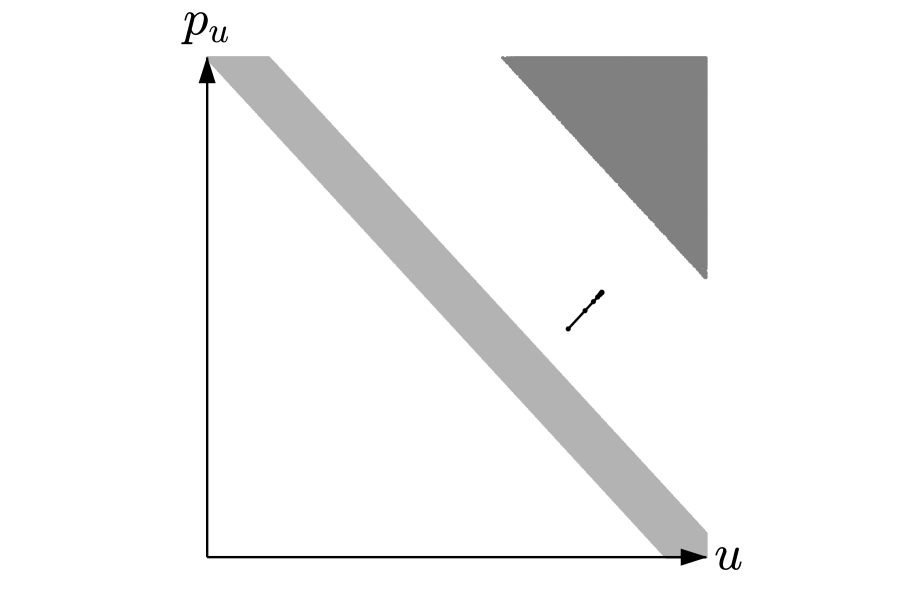
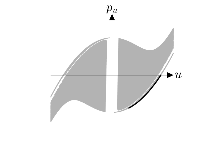
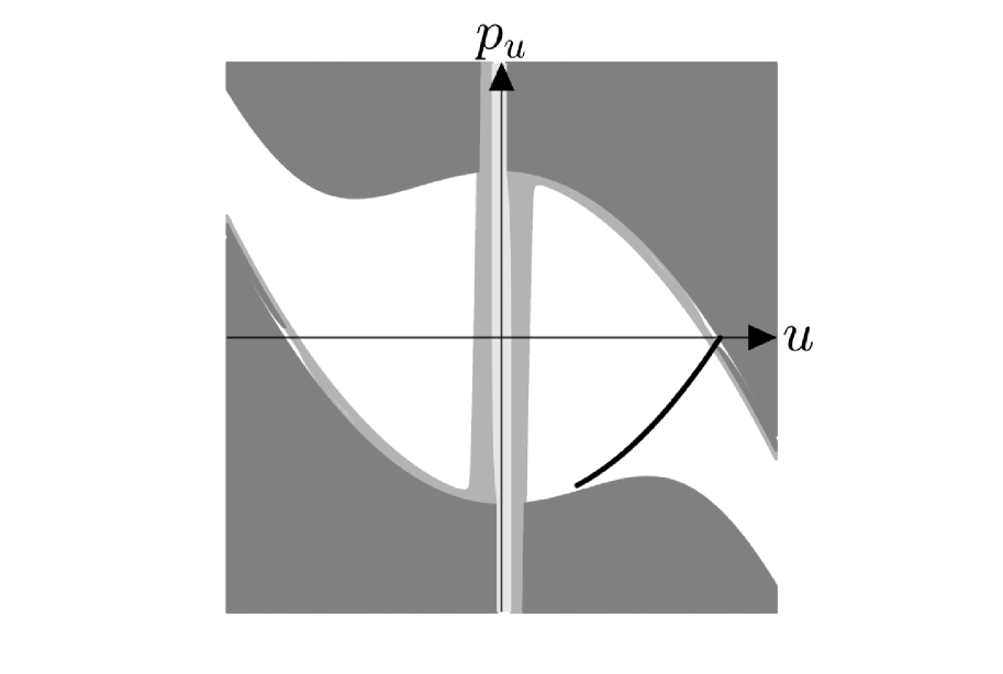
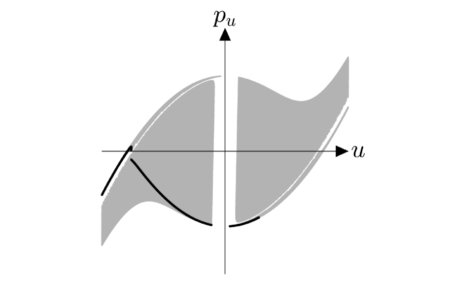
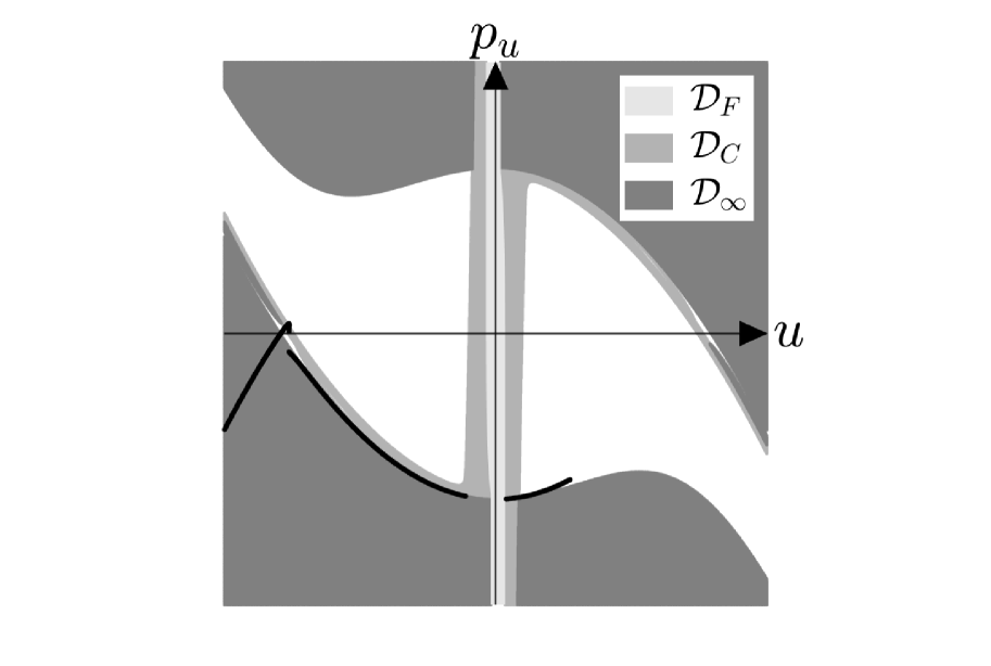
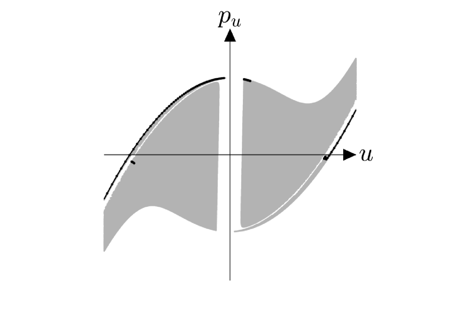
Figure 12: Constructing one branch of the unstable manifold of ${\bm{\hat{\upsilon}}}_{1}$. In the background there are the domain ${\cal D}$ and the forbidden regions ${\cal D}_{F},{\cal D}_{C},{\cal D}_{\infty}$ (left), the image of the map $\mathfrak{S}({\cal D})$ (right). The initial primary, drawn in the top left figure, is located in the smaller rectangle in Figure 9. Here, $\ell_{s}=348600$ $\mathrm{k}\mathrm{{}^{3}}\mathrm{m}\mathrm{/}{\mathrm{s}}^{2}$, $f=9.12\times 10^{-9}$ $\mathrm{k}\mathrm{m}\mathrm{/}{\mathrm{s}}^{2}$.

Figure 12 shows the first steps of the construction of a branch of the unstable manifold. The initial primary $V_{0}$ (top left) is first iterated once under the map (top right). Its image $V_{1}$ intersects the forbidden region ${\cal D}_{C}$ (middle left), and at the second iteration of $\mathfrak{S}$ three components are left (middle right), two of which lie in the $\{u<0\}$ half-plane. Again, their image $V_{2}$ intersects the forbidden regions ${\cal D}_{C}$, ${\cal D}_{\infty}$ (bottom left) and the number of components increases at the successive iteration (bottom right).

In Figure 13 we draw the four (disconnected) branches of the stable and unstable manifold of the fixed point $\widehat{{\bm{\upsilon}}}_{1}$.

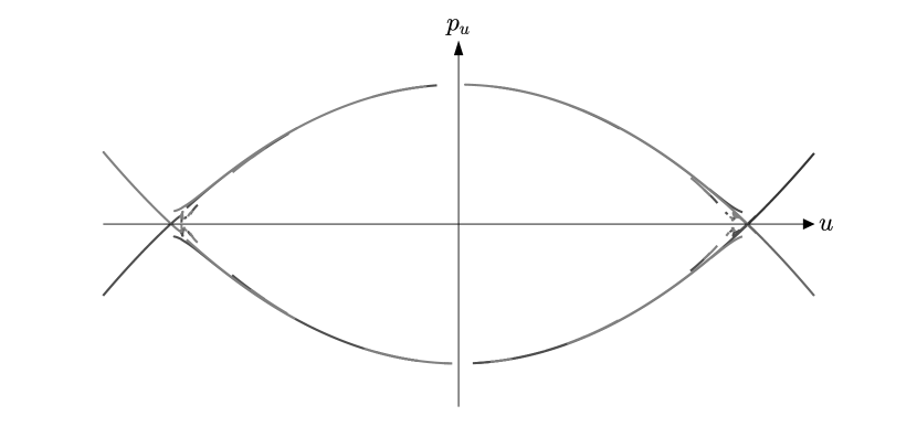
Figure 13: Stable and unstable invariant manifolds of ${\bm{\upsilon}_{1}}$.

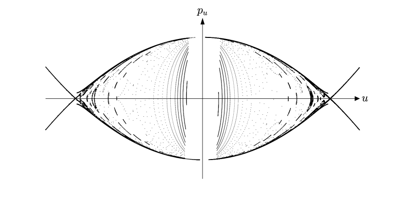
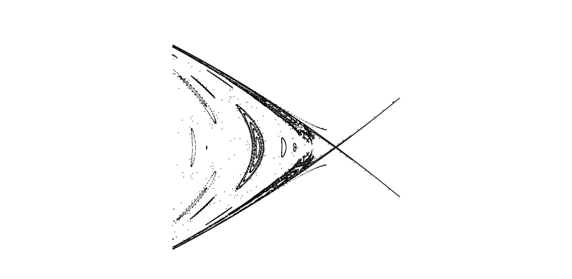
Figure 14: On the top we show a global picture of the Sun-shadow map, with $\ell_{s}=348600$ $\mathrm{k}\mathrm{{}^{3}}\mathrm{m}\mathrm{/}{\mathrm{s}}^{2}$, $f=9.12\times 10^{-9}$ $\mathrm{k}\mathrm{m}\mathrm{/}{\mathrm{s}}^{2}$. At the bottom we zoom in the region close to $\widehat{{\bm{\upsilon}}}_{1}$.

6 Conclusions and open questions

In this paper we have investigated the Sun-shadow dynamics, which is defined by patching together Kepler’s and Stark’s dynamics. After reviewing some relevant features of Stark’s problem, we prove the existence of a family of periodic orbits of brake type. Then, we introduce the Sun-shadow map, by fixing a quantity which is not conserved along the flow. This map is differentiable but is not area preserving. Its domain shows fine structures that underlie interesting phenomena when the map is iterated many times. There is numerical evidence that the fixed points $\widehat{{\bm{\upsilon}}}_{1}$, $\widehat{{\bm{\upsilon}}}_{2}$ related to the periodic orbits of brake type are hyperbolic; their invariant manifolds are constructed by an algorithm specifically created for this purpose. A global picture of this map is drawn in Figure 14, where an enhancement of the region close to the point $\widehat{{\bm{\upsilon}}}_{1}$ is also displayed. We observe evidence of regular and chaotic behaviour, with the presence of several islands: we checked that some of them surround periodic points. In the central region, where we have smaller values of $|u|$, the plotted points show a regular structure, similar to the one of the phase portrait in Figure 3. On the other hand, the regular behaviour seems to be lost in a neighbourhood of $\widehat{{\bm{\upsilon}}}_{1}$, along the stable and unstable branches of its invariant manifold.

This study opens some interesting questions about the Sun-shadow dynamics, which deserve to be further investigated. First, we may wonder whether the winding number associated to the trajectories corresponding to one iteration of the map is bounded from below, see Figure 11. Another interesting question is whether we can show that the islands appearing in Figure 14 correspond to invariant curves around fixed or periodic points. Moreover, we can ask ourselves whether Melnikov’s method can be adapted to prove the existence of chaotic dynamics in this case, where the invariant manifolds of the fixed points $\widehat{{\bm{\upsilon}}}_{1}$, $\widehat{{\bm{\upsilon}}}_{2}$ are made of several connected components (maybe infinitely many) due to the presence of the forbidden regions ${\cal D}_{\infty}$, ${\cal D}_{C}$, see Figure 12. Finally, possible future developments of this work are the extension of the Sun-shadow dynamics to the three-dimensional case, the inclusion of other perturbations (e.g. the Earth oblateness), and the study of the effect of the penumbra.

7 Acknowledgements

The authors have been partially supported by the MSCA-ITN Stardust-R, Grant Agreement n. 813644 under the H2020 research and innovation program. GFG and GB also acknowledge the project MIUR-PRIN 20178CJA2B “New frontiers of Celestial Mechanics: theory and applications”, and the GNFM-INdAM (Gruppo Nazionale per la Fisica Matematica).

Appendix A Appendix

Table 2: Stark’s problem: boundaries of the four regions in the $(\ell_{s},h_{s}/\sqrt{f})$ plane. The features of the trajectories in the $(x,y)$ plane are qualitatively described. $i$ is the imaginary unit.

Regions $I$, $II$	$\ell_{s}=-\mu$; $h_{s}/\sqrt{f}\in(0,+\infty)$
$V(v)$, $U(u)$ roots	${v}_{1}>0$, ${v}_{2}\in i\mathbb{R}$, ${u}_{1}=0$, ${u}_{2}\in i\mathbb{R}$
$v$,$u$ variable	$v\in[-{v}_{1},{v}_{1}]$, $u\in(-\infty,+\infty)$
trajectories type	two types: periodic, brake, passing through the origin;
	asymptotic to the periodic orbit in the future or in the past
Regions $I$, $IV$	$\ell_{s}=-\mu$; $h_{s}/\sqrt{f}\in(-\infty,0)$
$V(v)$, $U(u)$ roots	${v}_{1}>0$, ${v}_{2}\in i\mathbb{R}$, ${u}_{1}>{u}_{2}=0$
$v$, $u$ variable	$v\in[-{v}_{1},{v}_{1}]$, $u\in(-\infty,-u_{1}]\cup\{0\}\cup[u_{1},+\infty)$
trajectories type	two types: brake, periodic, passing through the origin;
	unbounded, self-intersecting, not encircling the origin
Regions $II$, $IV$	$\ell_{s}=(-\mu,\mu)$; $h_{s}/\sqrt{f}=-\sqrt{2(\mu+\ell_{s})}$
$V(v)$, $U(u)$ roots	${v}_{1}>0$, ${v}_{2}\in i\mathbb{R}$, ${u}_{1}={u}_{2}$, $u_{1},u_{2}>0$
$v$, $u$ variable	$v\in[-{v}_{1},{v}_{1}]$, $u\in(-\infty,+\infty)$
trajectories type	two types: periodic, brake; asymptotic to the
	periodic orbit in the future or in the past
Regions $II$, $III$	$\ell_{s}=\mu$; $h_{s}/\sqrt{f}\in(0,+\infty)$
$V(v)$, $U(u)$ roots	${v}_{1}>{v}_{2}=0$, ${u}_{1},{u}_{2}\in\mathbb{C}\setminus\mathbb{R}$
$v$, $u$ variable	$v\in[-{v}_{1},{v}_{1}]$, $u\in(-\infty,+\infty)$
trajectories type	two types: unbounded, not self-intersecting;
	unbounded with $y=0$ and $x\geq 0$
Region $II$	$\ell_{s}=\mu$; $h_{s}/\sqrt{f}\in(-\sqrt{2(\mu+\ell_{s})},0)$
$V(v)$, $U(u)$ roots	${v}_{1}=0$, $v_{2}\in i\mathbb{R}$, ${u}_{1},{u}_{2}\in\mathbb{C}\setminus\mathbb{R}$
$v$, $u$ variable	$v=0$, $u\in(-\infty,+\infty)$
trajectories type	unbounded with $y=0$ and $x\geq 0$
Region $IV$	$\ell_{s}=\mu$; $h_{s}/\sqrt{f}\in(-\infty,-\sqrt{2(\mu+\ell_{s})})$
$V(v)$, $U(u)$ roots	${v}_{1}=0$, ${v}_{2}\in i\mathbb{R}$, ${u}_{1}>{u}_{2}>0$
$v$, $u$ variable	$v=0$, $u\in(-\infty,-{u}_{1}]\cup[-{u}_{2},{u}_{2}]\cup[{u}_{1},+\infty)$
trajectories type	two types: brake, periodic, passing through the origin;
	unbounded, with $y=0$, $x>0$
Region $III$	$\ell_{s}\in(\mu,+\infty)$; $h_{s}/\sqrt{f}=\sqrt{-2(\mu-\ell_{s})}$
$V(v)$, $U(u)$ roots	${v}_{1}={v}_{2}$, $v_{1},v_{2}>0$, ${u}_{1},{u}_{2}\in\mathbb{C}\setminus\mathbb{R}$
$v$, $u$ variable	$v\in\{\pm v_{1}\}$, $u\in(-\infty,+\infty)$
trajectories type	unbounded, not self-intersecting, parabolic

Table 3: Stark’s problem: boundary points in the $(\ell_{s},h_{s}/\sqrt{f})$ plane. The features of the trajectories in the $(x,y)$ plane are qualitatively described. $i$ is the imaginary unit.

Regions $I$, $II$, $IV$	$\ell_{s}=-\mu$; $h_{s}/\sqrt{f}=0$
$V(v)$, $U(u)$ roots	${v}_{1}>0$, ${v}_{2}=0$, ${u}_{1}=0$, ${u}_{2}\in i\mathbb{R}$
$v$,$u$ variable	$v\in[-{v}_{1},{v}_{1}]$, $u\in(-\infty,+\infty)$
trajectories type	two types: periodic, brake, passing through the origin;
	asymptotic to the periodic orbit in the future or in the past
Regions $II$, $III$	$\ell_{s}=\mu$; $h_{s}/\sqrt{f}=0$
$V(v)$, $U(u)$ roots	${v}_{1}=0$, $v_{2}=0$, ${u}_{1},{u}_{2}\in\mathbb{C}\setminus\mathbb{R}$
$v$, $u$ variable	$v=0$, $u\in(-\infty,+\infty)$
trajectories type	unbounded with $y=0$ and $x\geq 0$
Regions $II$, $IV$	$\ell_{s}=\mu$; $h_{s}/\sqrt{f}=-\sqrt{2(\mu+\ell_{s})}$
$V(v)$, $U(u)$ roots	${v}_{1}=0$, ${v}_{2}\in i\mathbb{R}$, ${u}_{1}={u}_{2}$, $u_{1},u_{2}>0$
$v$, $u$ variable	$v=0$, $u\in(-\infty,+\infty)$
trajectories type	fixed point; asymptotic to the fixed point in
	the future and in the past with $y=0$, $x\geq 0$

References

- [1] V. V. Beletski. Space-flight trajectories with a constant-reaction accelerator vector. Translated from Kosmicheskie Issledovaniya, 2(3):408–413, 1964.
- [2] V. V. Beletski. Essays on the Motion of Celestial Bodies. Springer, Basel, 2001.
- [3] D. A. Cox. The arithmetic-geometric mean of gauss. L’Enseignement Mathématique, 30:275–330, 1984.
- [4] S. Ferraz Mello. Analytical study of the Earth’s shadowing effects on satellite orbits. Celestial Mechanics, 5:80–101, 1972.
- [5] D. Hobson. An Efficient Method for Computing Invariant Manifolds of Planar Maps. Journal of Computational Physics, 104:14–22, 1993.
- [6] C. Hubaux and A. Lemaître. The impact of Earth’s shadow on the long-term evolution of space debris. Celestial Mechanics and Dynamical Astronomy, 116:79–95, 2013.
- [7] C. Hubaux, A.-S Libert, N. Delsate, and T. Carletti. Influence of Earth’s shadowing effects on space debris stability. Advances in Space Research, 51:25–38, 2013.
- [8] Y. Kozai. Effects of the Solar-Radiation Pressure on the Motion of an Artificial Satellite. Smithsonian Contributions to Astrophysics, 6:109–112, 1960.
- [9] E. Lega and M. Guzzo. Three-dimensional representations of the tube manifolds of the planar restricted three-body problem. Physica D: Nonlinear Phenomena, 325:41–52, 2016.
- [10] M. L. Lidov. Secular effects in the evolution of orbits under the influence of radiation pressure. Translated from Kosmicheskie Issledovaniya, 7(4):467–484, 1969.
- [11] A. Milani, A. A. Nobili, and P. Farinella. Non-gravitational perturbations and satellite geodesy. IOP Publishing, Bristol, 1987.
- [12] P. Musen. The Influence of the Solar Radiation Pressure on the Motion of an Artificial Satellite. Journal of Geophysical Research, 65(5):1391–1396, 1960.
- [13] R. W. Parkinson, H. M. Jones, and I. I. Shapiro. Effects of Solar Radiation Pressure on Earth Satellite Orbits. Science, 131(3404):920–921, 1960.
- [14] P. J. Redmond. Generalization of the Runge-Lenz Vector in the Presence of an Electric Field. Physical Review, 133(5):1352–1353, 1964.
- [15] C. Simo. On the Analytical and Numerical Approximation of Invariant Manifolds. In Editions Frontières, editor, Modern Method in Celestial Mechanics, pages 285–329. Benest, D., Froeschle, C., Observatoire de la Côte d’azur, 1989.