Optics Design of Vertical Excursion Fixed-Field Alternating Gradient Accelerators

Abstract

Vertical excursion fixed-field alternating gradient accelerators can be designed with tunes that are invariant with respect to momentum and trajectories that are scaled images of each other displaced only in the vertical direction. This is possible using guiding fields that have a vertical exponential increase, with a skew quadrupole component in the magnet body and a solenoid component at the magnet ends. Because of the coupling this introduces, orbit and optics calculations and optimisation of parameters need to be performed numerically. In this paper, idealised magnetic fields are calculated from first principles, taking into account end fields. The parameter dependence of the optics and the dynamic aperture of the ring are calculated for the example of a ring with an approximately 25 m circumference that accelerates proton beams from 3 MeV to 12 MeV. The paper reports for the first time the design of such an accelerator lattice using tools specifically devised to analyse transverse coupled optics without the need for approximations.

I Introduction

The idea of a vertical excursion Fixed-Field Alternating Gradient accelerator (vFFA) [1, 2] can be traced back to the discovery of the original FFA concept [3, 4, 5], although relatively little emphasis was placed on the vFFA option at the time. In a vFFA, the beams move vertically when accelerated in contrast to the original FFA where the orbits stay in a horizontal plane. The idea has since been revived independently by Brooks, who has pointed out several potential applications of such a machine [6].

To avoid any confusion, we use the notation hFFA and vFFA in this paper to distinguish between the horizontal and vertical arrangements.

When used to accelerate electrons in the ultra-relativistic regime, a vFFA can deliver continuous electron beams because the path length is independent of momentum, in contrast with ordinary cyclotrons. Such a machine has been called an electron cyclotron [1]. Recently a continuous proton beam accelerator has been proposed by Mori [7] for the production of high power muon beams based on the vFFA concept.

The feature of a finite dispersion function only in the vertical direction is unique among particle accelerators. The momentum compaction factor is zero as a result of the zero horizontal dispersion function. The path length is independent of the beam momentum so that the beam dynamics behaviour is closer to that of a linear accelerator. This is advantageous for muon acceleration at ultra-relativistic energies in a muon collider or a neutrino factory. There is no need to ramp the magnetic field strength or to change the RF acceleration frequency according to the beam momentum. If adopted as a synchrotron radiation source, light rays of different radiation spectra are separated vertically because the beam momentum is a function of vertical position. The zero momentum compaction factor including higher order terms of momentum deviation also opens up novel lattice design strategies towards short bunch operation [8]. For crystalline beam formation in a ring accelerator, zero dispersion in the horizontal direction could eliminate the use of taper cooling [9]. These are just a few examples of possible vFFA applications. A practical feature is that the footprint of the main magnets in a vFFA is reduced compared to a cyclotron or an hFFA, although the magnets are taller.

Unlike an hFFA, a vFFA separates the shape of the ring (as seen from above) from the so-called scaling conditions. The scaling conditions are, first, the shape of orbits for different momenta in hFFAs are photographic enlargement of each other, whereas in vFFAs the orbits are identical apart from a vertical translation. Secondly, effective focusing strength normalized by the particle’s momentum is constant for all the momenta. Those two conditions make the transverse tune constant over the whole range of acceleration. The magnetic field variation in an hFFA, which applies to each field component, is

$$B/B_{0}=\left(r/r_{0}\right)^{k}$$ (1)

where $r_{0}$ is the reference radius measured from the machine centre and $B_{0}$ is the magnetic field at the reference radius. $k$ is the geometrical field index defined as $k=\left(r/B\right)\left(\partial B/\partial r\right)$, which determines the field strength as a function of the distance from the machine centre. In a vFFA the magnetic field satisfies the scaling conditions

$$B/B_{0}=\exp\big{(}m(y-y_{0})\big{)}$$ (2)

where $y_{0}$ is the reference position in the vertical coordinate and $B_{0}$ is the magnetic field at the reference position. $m$ is the normalised field gradient defined as $m=\left(1/B\right)\left(\partial B/\partial y\right)$. This does not involve the geometry of the ring. As long as stable optics exist, the ring shape can be arbitrary [10].

Note that there is a family of FFAs which do not obey the scaling conditions, referred to as ‘non-scaling’. However, here we consider only a vFFA design where the scaling conditions hold true.

vFFAs rely on a magnetic field where all three components increase exponentially in the vertical direction. As shown in section II, it is possible to create such magnetic fields with a semi-analytical approach consistent with Maxwell’s equations. With a proper combination of these magnets closed orbits and stable optics can be found corresponding to a ring accelerator.

As Brooks pointed out [6], the beams are predominantly confined by a skew quadrupole component in the middle of the lattice magnets. The particle motion in the horizontal and vertical planes is not independent. However the source of the coupling is not only from the skew quadrupole component in the magnet body. As described in section II, there is a potentially strong solenoid field at both ends of the magnet which introduces additional mixing between the horizontal and vertical motions. In fact, the maximum magnetic field is driven by this longitudinal end field in our design. When the magnet is long compared with the fringe field fall-off and the bending angle per cell is small, a 45 degree rotation of the physical horizontal and vertical coordinates is sufficient to decouple the particle motion, as in the case of [6]. This is not the case, however, when the magnet is short and the bending angle per cell is of the order of 10 degrees, which is the case for the majority of accelerator designs up to a few GeV and is discussed below. Edge focusing, weak focusing and higher order multipoles also contribute. The beams experience a mixture of normal and skew components as they pass through each cell.

The complication due to this mixing makes it challenging to derive essential accelerator parameters analytically such as transverse tune and beta functions. In this paper the stability of the optics and the beam dynamical behaviour in a vFFA are determined by numerical modelling. The $4{\times}4$ transfer matrix is obtained from particle tracking. The eigenvalues and eigenvectors of the matrix elements are used to analyse the coupled motion. Further particle tracking is used to explore the stable phase space volume.

Our future plan at the ISIS Neutron and Muon Source Facility aims for a proton driver of 1.2 GeV kinetic energy to provide 1.25 MW beam power with a ring of about 150 m circumference [11]. With vFFA optics, a reasonable choice for the ring would have a total of 25 cells, each of 6 m length. To support the design work, construction of a 25 m circumference vFFA with 10 focusing cells is being considered as a scaled-down, prototype ring. It is planned that this ring will use the ISIS Front End Test Stand (FETS) as an injector [12] and has therefore been provisionally accorded the name FETS-FFA.

The purpose of this paper is to discuss the procedure used in the design of the prototype vFFA. However the methodology can be applied to any similar vFFA, including the applications discussed above.

II Magnetic Field Model and Lattice Geometry

II.1 Magnet Field Model

In a vFFA, the scaling condition requires magnetic fields that increase exponentially in the vertical direction. In the following, the $x$-axis is horizontal, the $y$-axis is vertical and the $z$-axis is in the longitudinal direction. We set the (arbitrary) reference position $y_{0}=0$ in Eq. (2). The mid-plane of a vFFA rectangular magnet is defined where the horizontal coordinate is zero. The horizontal field component becomes zero when the current source of the magnetic field has mirror symmetry about the mid-plane. All three components of the magnetic field are described by a polynomial expansion to order $N$ in $x$ and the vertical field variation on the mid-plane is described by a function of $g(z)$:

$$B_{x}\left(x,y,z\right) =B_{0}\exp(my)\sum_{i=0}^{N}b_{xi}\left(z\right)x^{i},$$ (3)

$$B_{y}\left(x,y,z\right) =B_{0}\exp(my)\sum_{i=0}^{N}b_{yi}\left(z\right)x^{i},$$

$$B_{z}\left(x,y,z\right) =B_{0}\exp(my)\sum_{i=0}^{N}b_{zi}\left(z\right)x^{i}.$$

Maxwell’s laws can be used to derive the recursive relations between the coefficients

$$b_{x0}\left(z\right) =0,$$

$$b_{y0}\left(z\right) =g(z),$$

$$b_{z0}\left(z\right) =\frac{1}{m}\frac{dg}{dz},$$

and

$$b_{x,i+1}\left(z\right) =-\frac{1}{i+1}\left(mb_{yi}+\frac{db_{zi}}{dz}\right),$$

$$b_{y,i+2}\left(z\right) =\frac{m}{i+2}b_{x,i+1},$$

$$b_{z,i+2}\left(z\right) =\frac{1}{i+2}\frac{db_{x,i+1}}{dz}.$$

When a magnet is sufficiently long, in the middle of a magnet in the longitudinal direction where $g(z)$ can be taken as constant and all the derivatives of $g(z)$ taken as zero, Eq. (3) reduces to the standard multipole series expansion of $B_{x}=-B_{0}\exp\left(my\right)\sin\left(mx\right)$, $B_{y}=B_{0}\exp\left(my\right)\cos\left(mx\right)$, $B_{z}=0$. It is worth noting that, when it is expanded again as a series, normal multipoles and skew multipoles alternate in turn, e.g. the first term is a normal dipole, the second term is a skew quadrupole, the third term is a normal sextupole, the fourth term is a skew octupole as Eq. (II.1) shows. In practice, it suggests that the magnetic fields of Eq. (3) may be fabricated with a combination of normal and skew multipoles up to some orders.

$$-\frac{B_{x}}{B_{0}} = \exp\left(my\right)\sin\left(mx\right)$$

$$= 0+mx+\frac{m^{2}}{2!}\left(2xy\right)+\frac{m^{3}}{3!}\left(-x^{3}+3xy^{2}\right)$$

$$+ \frac{m^{4}}{4!}\left(-4x^{3}y+4xy^{3}\right)+...,$$

$$\frac{B_{y}}{B_{0}} = \exp\left(my\right)\cos\left(mx\right)$$

$$= 1+my+\frac{m^{2}}{2!}\left(-x^{2}+y^{2}\right)+\frac{m^{3}}{3!}\left(-3x^{2}y+y^{3}\right)$$

$$+ \frac{m^{4}}{4!}\left(x^{4}-6x^{2}y^{2}+y^{4}\right)+....$$

Fringe fields are an important feature of FFA optics, and in this study we chose to model the magnetic field with a hyperbolic tangent function,

$$g(z)=\frac{1}{2}\left[\tanh\left(\frac{z+M/2}{L}\right)-\tanh\left(\frac{z-M/2}{L}\right)\right]$$

where $M$ is the magnet length and $L$ is a parameter related to the fringe field extent. The field is symmetric with $g(z)=g(-z)$. More complicated field profiles will be considered as the hardware design matures. To illustrate the field profiles, the 3D magnetic fields are shown in Fig. 1 where the parameters of Table 1 are used. The order of polynomial $N$ is determined numerically by examining the convergence properties of the field and, where tracking is performed, the tune.

Table 1: Dimension and strength of the magnet model shown in Fig. 1.

Parameter	Value
Magnet length ($M$)	0.4 m
Fringe field extent ($L$)	0.2 m
$B_{0}$	1 T
Normalised field gradient ($m$)	1.28 m-1
Order of polynomials $N$ in Eq. (3)	10

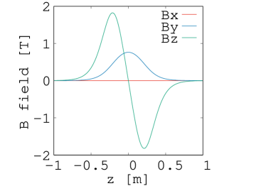
(a) $x=0$ m

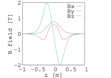
(b) $x=0.05$ m

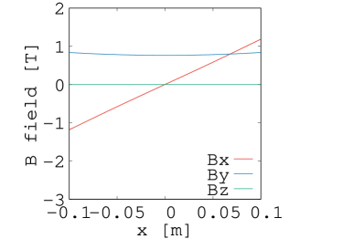
(c) $z=0$ m

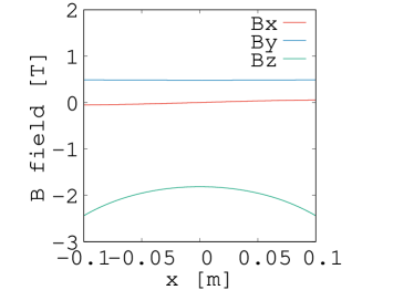
(d) $z=0.20$ m

Figure 1: $B_{x}$, $B_{y}$ and $B_{z}$ fields along the longitudinal axis ((a) and (b)) and the horizontal axis ((c) and (d)). The centre of the magnet is at $x=0,z=0$. In all cases, $y=0$. The field profiles in (b) are shown off-midplane to demonstrate a non-zero horizontal field $B_{x}$. The field profile in (d) is shown in the magnet end region to demonstrate a non-zero longitudinal field $B_{z}$.

In practice the vFFA magnet can be a superposition of many field maps described by Eq. (3). As long as the field strength changes according to $\exp(my)$ in all directions, the combined fields satisfy the scaling conditions. For example in section IV two such fields are superimposed with coordinates shifted in the horizontal direction by $+x_{c}$ and $-x_{c}$ respectively while maintaining the scaling conditions.

II.2 Number of Cells

Unlike ordinary accelerators where nonlinear magnetic fields exist either through fabrication errors or for correction of chromaticity around the central momentum, FFAs have strong nonlinearity in the magnetic fields in order to correct the chromaticity for the whole momentum range. Systematic nonlinear resonances should be avoided as much as possible. In addition, one of the eventual goals of our study is to accelerate high intensity beams in the vFFA where nonlinearity of the space charge potential is a concern, especially strong space charge driven 4^th order resonances [13].

To maximise the resonance-free space in the transverse tune diagram, the total number of cells is chosen as a multiple of 5. With this number of cells, systematic 5^th order resonances always coincide with integer resonances. It may be possible to find resonance-free regions of tune space 0.25 in cell tune away from 5^th order magnetic and 4^th order space charge resonances.

A superperiod structure can also be devised in a FFA ring by introducing several families of magnets. However, in our design, the ring comprises a simple repetition of a unit cell. We design the prototype 12  MeV ring with 10 cells.

II.3 Geometric Layout

FODO and FDF triplet lattices are considered in this paper. The lattice parameters are shown in Table 2. The geometry of the rings is described by a regular polygon with each side corresponding to a cell in the FDF triplet case or half-cell in the FODO case. Figures 2(a) and 2(c) may be used for guidance.

Table 2: Geometrical parameters of FODO and FDF triplet focusing lattices. Magnets were placed symmetrically about the centre of each side of the polygon.

Parameter	FODO	FDF Triplet
Bend angle per cell	36 deg	36 deg
Cell length	1.25 m (half)	2.50 m
Bd magnet length	0.50 m	0.24 m
Bf magnet length	0.50 m	0.40 m
Space between Bd and Bf	0.75 m	0.08 m
Bd horizontal wedge angle	-20 deg	0 deg
Bf horizontal wedge angle	+46 deg	0 deg
Double coil shift ($x_{c}$)	$\pm$0.02 m	$\pm$0.02 m
Fringe field extent ($L$)	0.15 m	0.20 m
Relative displacement ($x_{s}$)	$\pm$0.17 m	0 m
Tilt angle ($t_{f}$)	0 deg	0 deg

In the FODO lattice, a combination of a magnet with normal bending angle (Bf) and a magnet with reverse bend (Bd) is placed centrally on each side of the polygon. The number of polygon sides is twice the number of cells. Bd is displaced from the polygon edge by a distance $x_{s}$ radially towards the ring centre while Bf is displaced by $x_{s}$ radially away from the ring centre to follow the scalloped orbit of the beam.

The net bending angle per cell in the FODO is 36 degrees. As Bd bends the beams away from the ring centre, Bf must bend the beam by more than 36 degrees. To keep the beam round the gap centre of each magnet, a sector type magnet with curvature following the beam orbit is preferable. The sector-type magnet is modelled by splitting the Bf and Bd magnets into seven segments. The cell tune variation is less than $10^{-3}$ when seven or more segments are used, which was considered an acceptable precision for the model. Each segment is a rectangular type magnet but with finite angle between neighbouring segments. The fields of all the rectangular magnets are superimposed in the modelling.

In a FDF triplet lattice, Bf, Bd and Bf magnets are positioned symmetrically about the centre of each side of the polygon. All three magnets have rectangular shape. A sector magnet has not been considered to keep the magnet fabrication simple. As the bending angle per magnet is less than in the FODO lattice, the beam does not deviate so strongly from the magnet midplane. Lattice optimisation with the displacement parameter $\pm x_{s}$, the tilt angle $t_{f}$ of Bf with respect to Bd, magnet length and fringe field extent is discussed in section IV and the Appendix.

III Closed Orbit and Stable Optics

III.1 Finding a Closed Orbit

Given the lattice geometry, the normalised gradient $m$ and field strengths $B_{0d}$ and $B_{0f}$ from Eq. (3) of the Bd and Bf magnets respectively, the periodic orbit of a single cell (closed orbit) is numerically found by an algorithm minimising the difference between 4D transverse phase space coordinates at the entrance and the exit of the cell. The entrance and the exit are chosen at the centres of the long straight sections, where the field leakage from the magnets is at a minimum but not necessarily zero. The magnetic fields from the magnet in the cell and from magnets in the upstream and downstream cells are superimposed to account for this field leakage.

The closed orbits for the FODO lattice and FDF triplet are shown in Fig. 2. Magnetic fields along the orbit are also shown where $B_{x}$, $B_{y}$ and $B_{z}$ are defined with respect to the coordinate parallel to a side of the polygon.

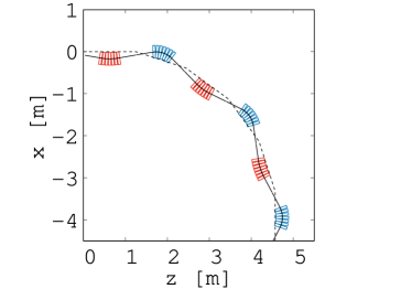
(a) FODO: orbit

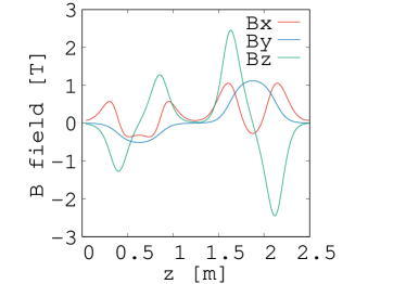
(b) FODO: fields

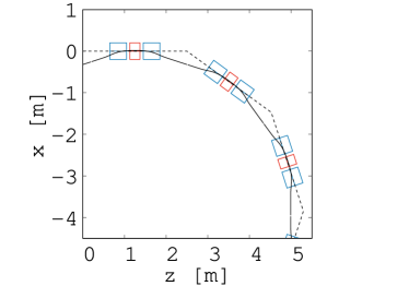
(c) FDF triplet: orbit

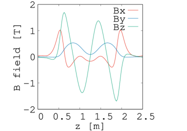
(d) FDF triplet: fields

Figure 2: Closed orbits for FODO (a) and FDF triplet lattices (c). The dashed line indicates the polygon with 20 sides for the FODO lattice and with 10 sides for the FDF triplet. Bd and Bf magnets are marked with by red and blue boxes respectively. In the FODO lattice, seven rectangular magnets mimic a sector magnet. Bd is shifted inward with respect to one side of polygon by $x_{s}$ and Bf is shifted outward by $x_{s}$. The magnetic fields along the orbit in a cell for 12 MeV beam energy are shown for FODO (b) and FDF triplet (d).

III.2 Orbits with Different Momenta

Because of the finite horizontal field in a vFFA, particles travelling at a fixed energy do not stay in a horizontal plane but experience an oscillation in the vertical direction as the beam goes round the ring. Orbits for different energies are displaced vertically, for example as the beam is accelerated. Projections of the closed orbits for different particle momenta, shown in Fig. 3, reveal interesting features. Since the magnetic field increases exponentially, the vertical projection shows that the orbit separation with a constant increase of momentum shrinks logarithmically.

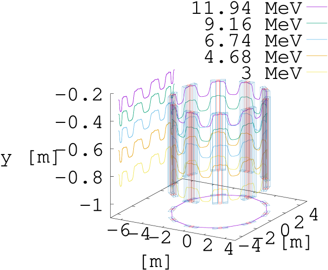
Figure 3: Closed orbits for different momenta in the FDF triplet lattice. The locations of the Bd and Bf magnets are indicated by red and blue boxes respectively. The ratio of magnet strength $B_{0d}/B_{0f}$=-0.20 and the value of the normalised field gradient $m$ is fixed at 1.28 m^-1. Path length is constant for the entire momentum range, in other words, the momentum compaction factor is zero.

Horizontal projections of the orbits are actually identical, despite the vertical shift, and this confirms the earlier observation that the momentum compaction factor is zero over the entire momentum range.

III.3 Finding Stable Optics

Once the closed orbit is found, the next step is to determine whether the motion around it is stable by calculating the transverse eigentunes. Particles are tracked through the cell with an offset in each transverse coordinate in order to determine the 4$\times$4 transverse transfer matrix $T$. This transfer matrix clearly shows non-zero off-diagonal matrix elements (e.g. $T_{13}$ and $T_{14}$) because of the skew quadrupole component from the body field and solenoid fields at the magnet ends. The former comes from the exponentially increasing field in Eq. (3).

Two transverse tunes, denoted by $q_{u}$ and $q_{v}$, are obtained as arguments of the conjugate pairs of complex eigenvalues of the 4$\times$4 transfer matrix $T$, The amplitude functions (the $\beta$-functions) of the FDF triplet lattice are calculated from the eigenvectors according to the Willeke-Ripken formalism [14] and are shown in Fig. 4.

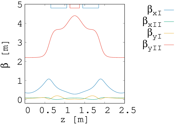
Figure 4: Beta functions $\beta_{xI}$, $\beta_{xII}$, $\beta_{yI}$, $\beta_{yII}$ according to the procedure by Willeke-Ripken [14]. The magnet positioning is shown at the top, the red box corresponding to the Bd magnet and the blue box to the Bf magnet.

In the following discussion, we will focus mainly on the FDF triplet lattice design.

IV Parameter search

IV.1 Orbit Control

In conventional accelerators, local orbit correction is provided by dipole magnets that are excited individually depending on the distortion along the beam trajectory. The orbit is corrected in the horizontal direction by a dipole magnet with a vertical field and in the vertical direction by a dipole with a horizontal field. In a vFFA, a vertical orbit corrector could be designed in the same way, but the horizontal orbit corrector may require a dipole magnet with a large gap, probably more than half a metre, spanning the orbit excursion in the vertical direction, and this would be challenging to implement.

The double coil design mentioned above enables horizontal orbit correction. Two pairs of coils, shifted horizontally with respect to their midplanes, can be excited with different currents. Tuning the currents can enable tuning of the profile of the vertical field along the horizontal direction while maintaining the scaling condition. The effect on cell tune is small as we expect from the usual method of orbit correction using dipole magnets. In Fig. 5, horizontal orbits are shown with different coil excitations together with the corresponding variation in tune. The orbit moves by several centimetres while the variation in cell tune is less than 0.01.

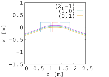
(a) orbit shift in FDF triplet

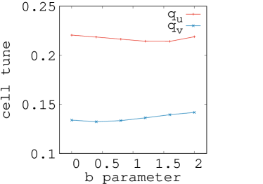
(b) tune shift in FDF triplet

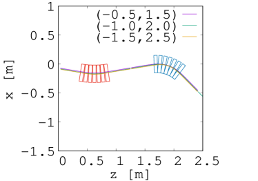
(c) orbit shift at Bd in FODO

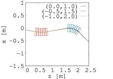
(d) orbit shift at Bf in FODO

Figure 5: Orbit shift controlled by a double coil design. A bracket $(b,1-b)$ indicates the relative excitation of outer coil $b$ to inner coil $1-b$. The total excitation is kept at unity. By having different excitation patterns of outer and inner coils, the orbit position can be controlled with little change of tune.

IV.2 Optics Optimisation

In an hFFA, two tuning parameters are used to change the orbit and optics: the field index $k$, defined in Eq. (1), and the ratio of the field strengths of the normal (Bf) and reverse (Bd) bending magnets. The field index $k$ defines the focusing and defocusing strength of the magnet body. The field ratio controls the ratio of normal and reverse bending fields, which enables manipulation of the orbit scalloping and hence focusing and defocusing action at the edge of the magnets.

Similarly in a vFFA, the normalised field gradient $m$ and the ratio of the field strengths of Bf and Bd are the main parameters used to adjust optical features. Figure 6 shows the area in $(m,B_{0d}/B_{0f})$ space that gives stable optics and significant dynamic aperture for the FDF triplet lattice. The dynamic aperture on the corresponding $(q_{u},q_{v})$ space is also shown, where $q_{u}$ and $q_{v}$ are the tunes in the decoupled space $(u,p_{u},v,p_{v})$ [15].

Dynamic aperture, the region of phase space in which the beam can be transported around the ring, is estimated by particle tracking. Particles are tracked having initial values $(u,p_{u},v,p_{v})=(\sqrt{iu_{0}},0,0,0)$ and $(u,p_{u},v,p_{v})=(0,0,\sqrt{jv_{0}},0)$. $u_{0}$ and $v_{0}$ are chosen to correspond to a single particle amplitude of $A_{0}=5\,\pi$ mm mrad in normalised space and $i$ and $j$ are positive integers. The dynamic aperture is estimated as $A=(i_{\mathrm{max}}+j_{\mathrm{max}})A_{0}$ where $i_{\mathrm{max}}$ and $j_{\mathrm{max}}$ correspond to the largest values of $i$ and $j$ for which the particle survives 100 turns. A more detailed study of dynamic aperture is described in section V.

Similar figures for slightly different geometries are shown in Appendix A. The baseline parameters of the FDF triplet lattice, $B_{0d}/B_{0f}=-0.20$ and $m=1.28$ m^-1, were chosen for further study, owing to the excellent dynamic aperture.

(a) $m$ and $B_{0d}/B_{0f}$ space.

(b) $q_{u}$ and $q_{v}$ space.

Figure 6: Stable area in $m$ and $B_{0d}/B_{0f}$ space and $q_{u}$ and $q_{v}$ space. The colour code indicates the maximum amplitude of betatron oscillation $A=(i_{\mathrm{max}}+j_{\mathrm{max}})A_{0}$ where $A_{0}=5\pi$ mm mrad in normalised space, $i_{\mathrm{max}}$ and $j_{\mathrm{max}}$ are the indices corresponding to the largest value of $i$ for $u$ space or $j$ for $v$ space for which the particle survives 100 turns.

IV.3 Edge Focusing

During the process of identifying the triplet configuration and physical dimension of the magnets, the edge focusing can be adjusted in simulation by moving the magnets. We have looked at the effect on the area of stable optics coming from two variations: one through the tilt angle $t_{f}$ of Bf magnets with respect to Bd magnet, and the other from the relative horizontal displacement, $x_{s}$, between the Bd and Bf magnets.

Figure 7 shows the stable area when $t_{f}$ changes from -2 to +6 degrees. A positive angle indicates Bf is relatively more aligned with the orbit. Figure 8 shows the stable area when $x_{s}$ changes from -0.04 to +0.04 m. A positive displacement indicates Bf moves away from the ring centre and Bd moves towards the ring centre. With a tilt imposed on Bf, the range of $m$ giving stable optics is reduced. With a displacement $x_{s}$, a stronger correlation between $m$ and $B_{0d}/B_{0f}$ appears.

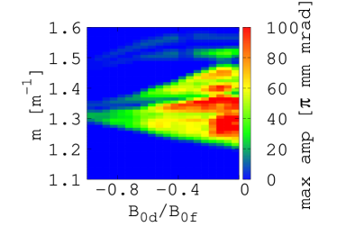
(a) $t_{f}$=-2 deg

(b) $t_{f}$=-2 deg

(c) $t_{f}$=0 deg

(d) $t_{f}$=0 deg

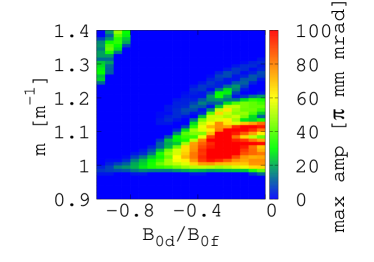
(e) $t_{f}$=2 deg

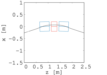
(f) $t_{f}$=2 deg

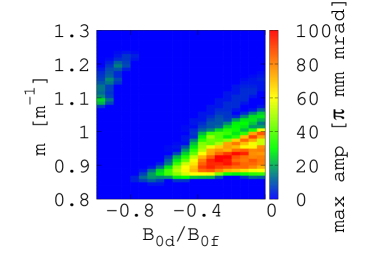
(g) $t_{f}$=4 deg

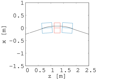
(h) $t_{f}$=4 deg

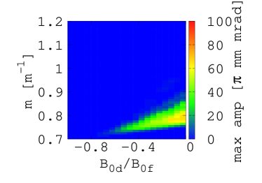
(i) $t_{f}$=6 deg

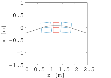
(j) $t_{f}$=6 deg

Figure 7: Stable area in $m$ and $B_{0d}/B_{0f}$ space depending on the tilt angle $t_{f}$ of Bf with respect to Bd and representative orbit for each case. Parameters of the representative orbits are listed in Table 3.

Table 3: Parameters of the representative orbits in Fig. 7.

$t_{f}$ [deg]	$B_{0d}/B_{0f}$	$m$ [m-1]	$q_{u}$	$q_{v}$
-2	-0.20	1.42	0,2285	0.1577
0	-0.20	1.28	0.2141	0.1394
2	-0.20	1.10	0.2264	0.1048
4	-0.20	0.93	0.2224	0.0736
6	-0.20	0.76	0.2164	0.0386

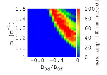
(a) $x_{s}$=-0.04 m

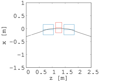
(b) $x_{s}$=-0.04 m

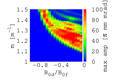
(c) $x_{s}$=-0.02 m

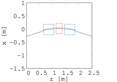
(d) $x_{s}$=-0.02 m

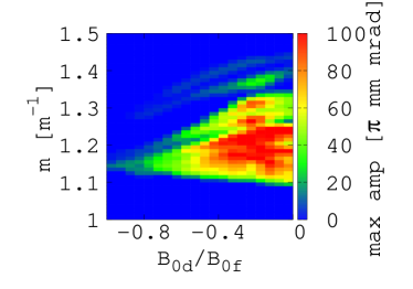
(e) $x_{s}$=0.0 m

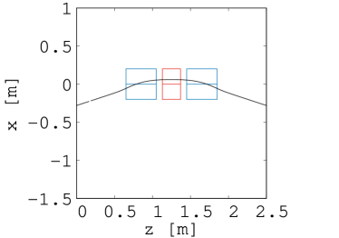
(f) $x_{s}$=0.0 m

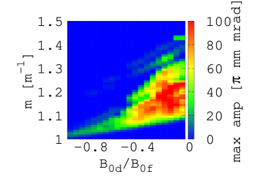
(g) $x_{s}$=0.02 m

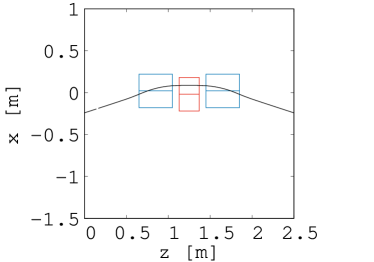
(h) $x_{s}$=0.02 m

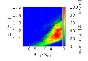
(i) $x_{s}$=0.04 m

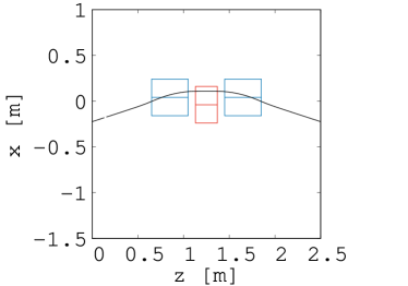
(j) $x_{s}$=0.04 m

Figure 8: Stable area in $m$ and $B_{0d}/B_{0f}$ space depending on radial displacement $x_{s}$ of Bf with respect to Bd and representative orbit for each case. Parameters of the representative orbits are listed in Table 4.

Table 4: Parameters for the representative orbits in Fig. 8.

$x_{s}$ [m]	$B_{0d}/B_{0f}$	$m$ [m-1]	$q_{u}$	$q_{v}$
-0.04	-0.40	1.44	0.2266	0.1131
-0.02	-0.40	1.31	0.2245	0.1133
0.00	-0.40	1.22	0.2220	0.1147
+0.02	-0.40	1.14	0.2342	0.1089
+0.04	-0.40	1.10	0.2259	0.1155

V Aperture

V.1 Dynamic Aperture

Dynamic aperture is estimated by particle tracking, but it is not straightforward to give a precise interpretation of the concept when the optics between the two transverse planes is coupled. Two steps were considered to provide an estimate that would be practically useful for accelerator design. As in the algorithm described above, particles were tracked having initial coordinate values $(x,p_{x},y,p_{y})=(ix_{0},0,0,0)$ and $(x,p_{x},y,p_{y})=(0,0,jy_{0},0)$ with respect to the closed orbit for a number of integer values of $i$ and $j$. This gives an estimate of the horizontal and vertical phase space where beams can be injected into the ring. Because of the coupling between the two planes, particles starting in one physical plane explore the 4D phase space, and do not remain in the 2D sub-space, but may not exhaustively explore the full 4D region. Figure 9 shows the surviving particles. To investigate the dependence of this dynamic aperture estimate on the number of turns, results with a different number of tracking turns are superimposed in the plots. The figure shows that there is only a small difference between the dynamic aperture defined by tracking for 100 turns and 1000 turns and almost no difference if the number of turns is more than 1000.

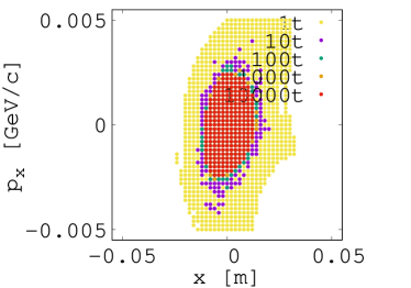
(a) $x$-$p_{x}$

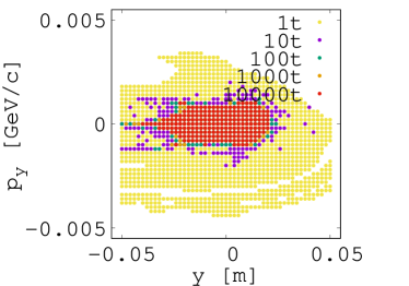
(b) $y$-$p_{y}$

Figure 9: Dynamic aperture in physical $x$-$p_{x}$ and $y$-$p_{y}$ planes. Results from tracking through a different number of turns: 1, 10, 100, 1000, 10000 turns are superimposed. The dynamic aperture defined by tracking for 100 turns and 1000 turns has only a small difference and converges when the number of turns is more than 1000.

In order to explore the accepted phase space more thoroughly, particles were tracked having random initial position and momentum in the 4D phase space. The results of the first step help to define the appropriate volume in 4D phase space where the particles should be randomly allocated: it should be large enough to cover the entire dynamic aperture. The ability of each particle to survive when tracked for 1000 turns of the ring is checked. The 4D phase space coordinates of the surviving particles define the 4D phase space volume and we identify dynamic aperture through projections onto the $u$-$p_{u}$ and $v$-$p_{v}$ linearly decoupled 2D phase spaces [15]. The coordinates of the particles surviving after tracking are also plotted. We assume that if the phase space area before and after the tracking have approximately the same shape and size, we are assured that the dynamic aperture defined above is stable and consistent, as shown in Fig. 10. In either plane, the normalised dynamic aperture is about 30 $\pi$ mm mrad. Projections of the 4D phase space volume to other planes are also depicted.

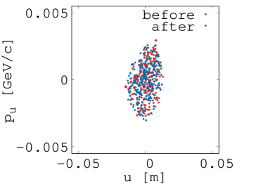
(a) $u$-$p_{u}$

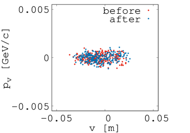
(b) $v$-$p_{v}$

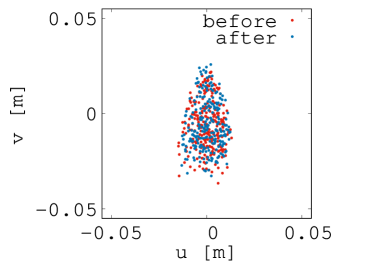
(c) $u$-$v$

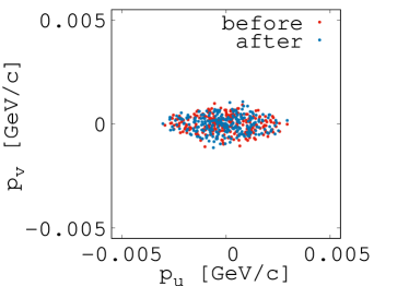
(d) $p_{u}$-$p_{v}$

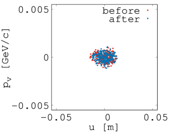
(e) $u$-$p_{v}$

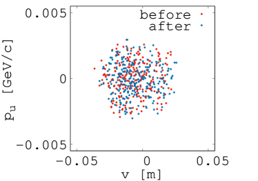
(f) $v$-$p_{u}$

Figure 10: Dynamic aperture defined by surviving particles in 4D space after 1000 turns. Red dots show the initial coordinates and blue dots are the final coordinates. Projections onto the decoupled spaces ((a) $u$-$p_{u}$ and (b) $v$-$p_{v}$) show that normalised dynamic aperture is estimated to be about 30 $\pi$ mm mrad. Projections of the 4D phase space volume onto other planes are also depicted.

V.2 Physical Aperture

Knowing the normalised dynamic aperture is about 30$\pi$ mm mrad, the mechanical aperture as well as beam core emittance after multi-turn painting injection are defined in Table 5. To convert un-normalised emittance at 3 MeV to beam size, values $\beta_{xI,\mathrm{max}}$=1.0 m and $\beta_{yII,\mathrm{max}}$=4.6 m are used according to Fig. 4. Contributions to the beam size from other planes are ignored since $\beta_{xII,\mathrm{max}}$ and $\beta_{yI,\mathrm{max}}$ are relatively small.

Table 5: Specifications of beam core emittance and mechanical aperture.

	normalised	un-normalised	$x$ size	$y$ size
	[$\pi$ mm mrad]	[$\pi$ mm mrad]	[mm]	[mm]
Beam core	5 – 10	62.5 – 125	8 – 11	17 – 24
Collimator
aperture	10 – 20	125 – 250	11 – 16	24 – 34
Chamber
aperture	–	–	$\pm$30	$\pm$350

VI Summary

In designing a vFFA, it is necessary to take into account coupling in the transverse planes, both for calculation of optics and optimisation of accelerator parameters. Strong coupling arises from the skew quadrupole components in the vFFA magnet body and also from longitudinal field components in the end fields. In this paper, we have employed tools to properly analyse these coupled optics. Assuming an idealised magnetic field model that satisfies Maxwell equations and has field strength increasing exponentially in the vertical direction, a design procedure has been established, with parameters such as the normalised field gradient $m$ and the ratio of Bd and Bf field strengths used to tune the optics. A prototype vFFA, accelerating proton beams from 3 MeV to 12 MeV, was used as an example. The design procedure is applicable to any vFFA since no approximation – such as small bending angle per cell – was made. An optics solution was found that is robust against small variation of parameters and gives large dynamic aperture.

Appendix A Benchmark of Simulation Codes

The design of the lattice has been performed throughout with SCODE+ [16]. This code was benchmarked against two other codes: FixField (previously named JBT) [17] and OPAL [18] comparing eigentunes as shown in Table 6. Eigentunes are constant for the whole range of momentum as expected.

Table 6: Comparison of results from three different codes.

	$q_{u}$	$q_{v}$
SCODE+	0.2178	0.1342
FixField	0.2198	0.1335
OPAL	0.2199	0.1340

Appendix B Stability of Lattices with Slightly Different Geometry

The stability of other lattices with slightly different geometry has also been investigated. Figures 11, 12 and 13 show the effect of varying the lengths of the Bd and Bf magnets and fringe field extent respectively. There is a non-zero drift space between the Bd and Bf magnets into which the overlapping fringe fields penetrate.

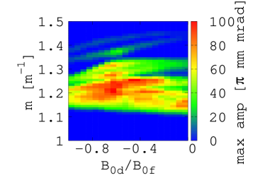
(a) Bd=0.16 m

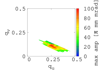
(b) Bd=0.16 m

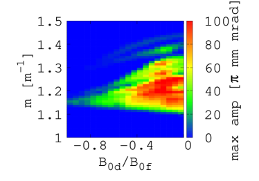
(c) Bd=0.24 m

(d) Bd=0.24 m

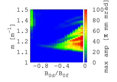
(e) Bd=0.32 m

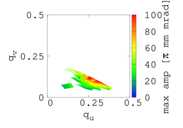
(f) Bd=0.32 m

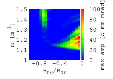
(g) Bd=0.40 m

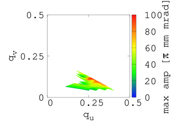
(h) Bd=0.40 m

Figure 11: Stable area in $m$ and $B_{0d}/B_{0f}$ space and in $q_{u}$ and $q_{v}$ space depending on the length of Bd.

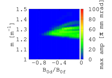
(a) Bf=0.24 m

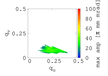
(b) Bf=0.24 m

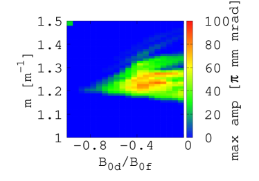
(c) Bf=0.32 m

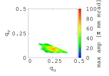
(d) Bf=0.32 m

(e) Bf=0.40 m

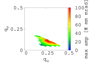
(f) Bf=0.40 m

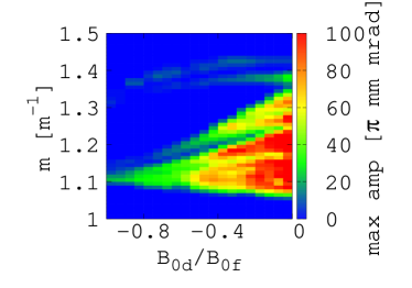
(g) Bf=0.48 m

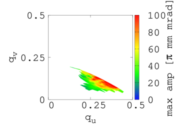
(h) Bf=0.48 m

Figure 12: Stable area in $m$ and $B_{0d}/B_{0f}$ space and in $q_{u}$ and $q_{v}$ space depending on the length of Bf.

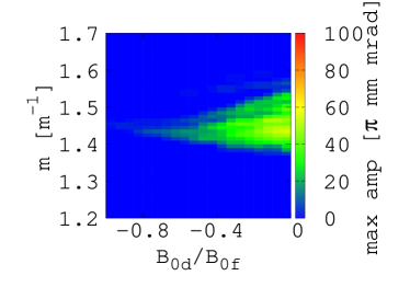
(a) L=0.150 m

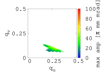
(b) L=0.150 m

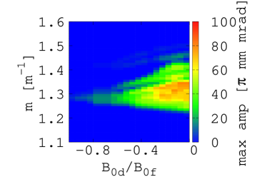
(c) L=0.175 m

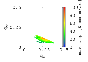
(d) L=0.175 m

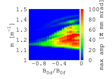
(e) L=0.200 m

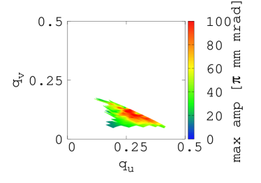
(f) L=0.200 m

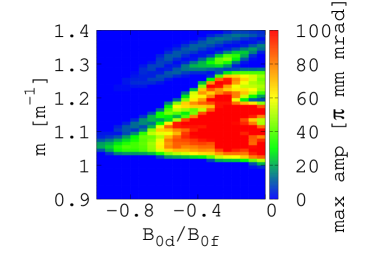
(g) L=0.225 m

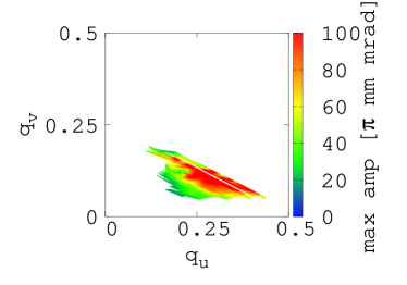
(h) L=0.225 m

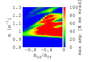
(i) L=0.250 m

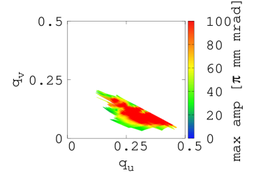
(j) L=0.250 m

Figure 13: Stable area in $m$ and $B_{0d}/B_{0f}$ space and in $q_{u}$ and $q_{v}$ space depending on the fringe field extent $L$.

References

- [1] T. Ohkawa, Bull. APS 30 (1955) 20.
- [2] J. Teichmann, Sov. J. At. Energ. 12 (1963) 507.
- [3] T. Ohkawa, Proc. Annual meeting of JPS (1953).
- [4] K. R. Symon, D. W. Kerst, L. W. Jones, L. J. Laslett, and K. M. Terwillinger, Phys. Rev. 103 (1956) 1837.
- [5] A. A. Kolomensky and A. N. Lebedev, Theory of Cyclic Accelerators (North-Holland, Amsterdam, 1966), p. 332.
- [6] S. Brooks, Phys. Rev. ST Accel and Beams 16 (2013) 084001.
- [7] Y. Mori, Y. Yonemura and H. Arima, Memoirs of the Faculty of Engineering, Kyushu University, Vol.77, No.2, December 2017.
- [8] I. Martin, et. al., Phys. Rev. ST Accel and Beams 14 (2011) 040705.
- [9] M. Ikegami, H. Sugimoto, H. Okamoto, Journal of the Physical Society of Japan Vol. 77, No. 7, July, 2008, 074502.
- [10] J.-B. Lagrange, et. al., Proc. of International Particle Accelerator Conference 2019, TUPTS068 (2019) 2075.
- [11] J. Thomason, https://www.isis.stfc.ac.uk/Pages/ isis-ii-working-group-report16266.pdf
- [12] A. Letchford, et. al., Proc. of International Particle Accelerator Conference 2015 (2015) 3959.
- [13] S. Machida, Nuclear Instruments and Methods in Physics Research A384 (1997), 316.
- [14] F. Willeke and G. Ripken, AIP Conf. Proc. 184 (1989) 758.
- [15] G. Parzen, acc-phys/9510006 31 Oct 1995 - arXiv.
- [16] S. Machida, ICFA BD Newsletter 43 Ed. C. R. Prior (2007) 54.
- [17] J-B. Lagrange et. al., JINST 13 (2018) P09013.
- [18] A. Adelmann, et. al., https://arxiv.org/abs/1905.06654, 2019.
Acknowledgements.
We wish to acknowledge fruitful discussion with S. J. Brooks and the support of members of the ISIS Accelerator and Design Divisions. We also thank C. R. Prior for careful reading of the manuscript.Appendix A Benchmark of Simulation Codes