Experimental demonstration of multimode microresonator sensing by machine learning

Abstract

A multimode microcavity sensor based on a self-interference microring resonator is demonstrated experimentally. The proposed multimode sensing method is implemented by recording wide band transmission spectra that consist of multiple resonant modes. It is different from previous dissipative sensing scheme, which aims at measuring the transmission depth changes of a single resonant mode in a microcavity. Here, by combining the dissipative sensing mechanism and the machine learning algorithm, the multimode sensing information extracted from a broadband spectrum can be efficiently fused to estimate the target parameter. The multimode sensing method is immune to laser frequency noises and robust against system imperfection, thus our work presents a great step towards practical applications of microcavity sensors outside the research laboratory. The voltage applied across the microheater on the chip was adjusted to bring its influence on transmittance through the thermo-optic effects. As a proof-of-principle experiment, the voltage was detected by the multimode sensing approach. The experimental results demonstrate that the limit of detection of the multimode sensing by the general regression neural network is reduced to 6.7% of that of single-mode sensing within a large measuring range.

I INTRODUCTION

Optical microphotonic sensors have excellent performance in terms of high responsivity, high sensitivity, and small foot-print (Jiang et al., 2020; Qian et al., 2018; Xue et al., 2019). One specific class of the microphotonic sensors, the so-called microcavity sensor supporting whispering gallery modes (WGMs), has attracted much research interest in recent years (Song, 2019; Zou et al., 2012; Chen et al., 2017; Zhang et al., 2017; Qin et al., 2019). With ultrahigh optical quality (Q) factors and ultrasmall mode volume, strongly localized WGMs lead to significant enhancement of light-matter interaction. So the environment perturbations, such as pressure, temperature, and force, could be detected with great sensitivity in WGM sensors. Typical microcavity sensing is implemented by measuring the resonant spectral changes, including the induced changes in resonant frequency, spectrum linewidth, and transmission depth (Foreman et al., 2015; Zhang et al., 2018; Zhi et al., 2017; La Notte et al., 2014). In conventional waveguide-coupled WGM sensors, the reactive interaction could only induce a frequency shift, which could be detected by high precision scanning lasers. Due to the limited scanning range and slow scanning rate, only a single optical resonance was measured to perform the sensing in most previous studies (La Notte et al., 2014).

However, the single-mode sensing performance might be restricted with the single information channel (Foreman et al., 2015; Zhang et al., 2018). In a WGM microcavity, various WGMs in wavelength are present with different azimuthal mode numbers, polarizations, quality factors, and so on. Generally speaking, these WGMs provide diverse sensing modalities. They are just like different sensing information collected by multiple sensors in the another sensing scene, where a target parameter is also detected by multiple sensor sources. By the aid of the existing sensor fusion technology, these different informations from multiple sensors could be effectively merged so that the resulting target parameter has less uncertainty than would be possible when these sensors were used individually (Khaleghi et al., 2013). Therefore, the sensing performance can be improved significantly by employing multiple WGMs, since the information that associate with other high-Q resonances are collected (Zhu et al., 2010, 2011; Kim et al., 2012; Yi et al., 2010; Mallik et al., 2018). In practice, there are two challenges to preventing such multimode sensing: (1) As noted above, scanning a wide range spectrum is a time-consuming process and also demanding a high-cost scanning laser. Besides, the laser frequency may be not stable and the cavity frequencies are also sensitive to thermal fluctuations (Zhu et al., 2011). (2) The responses of different WGMs to an unknown target parameter are different in general. This is due to the material and geometry dispersion of the microcavity WGMs, and also wavelength-dependent light-matter interaction. Without the sensing fusion algorithm, it is also difficult to estimate a parameter by measuring the responses of different WGMs. Therefore, the analysis of the full spectrum is regarded as time- and resource-consuming.

In this work, self-interference microring resonator (SIMRR) based multimode sensing is experimentally demonstrated. With the help of the dissipative sensing mechanism (Ren et al., 2016, 2019), a machine learning algorithm is used to fuse the multimode sensing data of a SIMRR. Because dissipative sensing is robust against frequencies noises, transmission depths of multiple resonant modes or all the intensity samples in the spectra, instead of their resonant frequencies, are considered as the sensing data. The SIMRR based multimode sensing principle has been theoretically proposed in Ref. (Hu et al., 2020). By probing the experimental system with a broadband laser source, these transmission depths of multiple resonant modes or full spectra are easily collected for training the artificial neural network (ANN) and estimating the object parameter. The trained ANN develops a prediction model. After the model is validated with the test set, its output is the “estimated” measurement result. It is worth noting that the spectra are not fitted in all data processing. Compared with the single-mode dissipative sensing, the SIMRR-based multimode sensing method improves the detecting accuracy considerably. The proposed method has great potential to offer a simple, robust, and high-sensitive sensing platform with low detecting cost.

II MUlTIMODE SENSING MECHANISM

The conventional add-drop microring resonator (ADMRR) consists of a microring resonator sandwiched between two parallel waveguides. In the typical amplitude transmittance of an ADMRR, a Lorentzian line shape is periodically repeated along the wavelength axis. Owing to almost the same spectral shifts in multiple resonances, it is often used to monitor the target parameter by measuring a resonant frequency shift, which is referred to as dispersive sensing. As demonstrated in our previous works (Ren et al., 2016, 2019; Hu et al., 2020; Wan et al., 2018), the SIMRR’s spectrum shows a feature of modulated extinction ratio over a large wavelength range, and the SIMRR is more robust against the laser frequency noises by converting frequency shift into changing of extinction ratio. The dissipative sensing based on SIMRR is enhanced by the Vernier effect due to the interference effect.

Therefore, the SIMRR-based multimode sensor is taken as an example, and the principle of the proposed multimode microcavity sensor is explained. As shown in Fig.1(a), the SIMRR consists of is a microring resonator that is coupled by a sensing arm waveguide two times. When a SIMRR is used as a sensor, the sensing arm waveguide is exposed to the target analyte to be detected. The sensing target can trigger the phase shift with different wavelengths under an optical path of the sensing arm waveguide. Eventually, distinct phenomena are exhibited in its transmission spectra, including the modulated transmission depth and spectrum linewidth. Its typical transmittance is displayed in the inset of Fig.1(a). In contrast to the ADMRR, the SIMRR shows a strong wavelength-dependent response (Feng et al., 2017; Ma et al., 2019). Although optical modes with different mode family, polarization, and orbital angular momentum can be excited in a WGM microcavity, the multimode sensing method is mainly hindered by the difficulty of full-spectrum analysis employing a frequency tracking method. Consequently, the existing WGM sensing methods, including dispersive and dissipative sensing, always focus on measuring the spectral change at a single resonance and results in the throw away of spectral shift data analysis in other resonances.

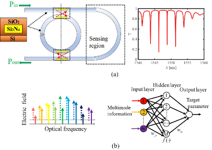
Figure 1: The proposed multimode sensing mechanism. (a) Structural diagram of a SIMRR-based sensor design and typical amplitude transmittance of a SIMRR. (b) An ANN assisted multimode sensing information fusion for predicting the target parameter.

Based on previous efforts on the single-mode dissipative sensing, the multimode sensing has been theoretically investigated in SIMRR-based sensor (Hu et al., 2020). Theoretical studies predict a significant enhancement of the detection accuracy. The single-mode sensing can be performed with different sensitivity based on the spectral change of each resonance. These sensitivities have to be estimated and accounted for in the process of estimating an eventual result. Therefore, one key issue is how to merge the sensing information from multiple resonances. In the sensor fusion technology, the neural network is particularly well suited for the combination of multiple sensing information (Khaleghi et al., 2013; Yu and Fan, 2011; Hall and Llinas, 1997; Dong et al., 2009; Bishop, 1995). Hence, we propose the supervised machine learning algorithm to fuse these multimode sensing informations. As shown in Fig.1(b), a back propagating-ANN (BP-ANN) is used to merge these transmission depth changes from multiple resonances. The multimode fusion model based on BP-ANN is built to estimate the target parameter. In the input layer, the input variables are more accurately described as an input set, since it generally consists of multiple independent variables (multiple transmission depth changes from multiple resonances), rather than a single value. A hidden layer is located between the input and output layers of the algorithm, where the function applies weights $w_{ji}$ to the inputs and directs them through an activation function $f(\cdot)$ as its output. In the output layer, the ultimate output is the summation of the product of the output signals in the hidden layer and another weight factor ($w_{m}$), and it is the estimated value of the target parameter.

The detailed process of implementation is as follows. Firstly, the related original data, including training and test sets, are collected for the BP-ANN. To train the network, the supervised learning algorithm requires a training set of paired inputs and known output labels. Then, the training set needs to be collected in advance. That is to say, many groups of transmission depths of multiple resonances are experimentally collected with known target parameter values before the measurement is started. After this, the actual measurement is performed by the SIMRR-based sensor, and an additional group of transmission depths is collected as the test set. Secondly, the network is trained by a back-propagation algorithm, which adjusts weights according to the gradient descent method (Bishop, 1995). The training process is completed after the training goal error is achieved. The purpose of the training is to establish the nonlinear mapping relationship between the input variables (a group of transmission depths) and the output variable (corresponding target parameter). Finally, the generalization ability of the trained network is investigated. The test set is input into the trained network, and the eventual measurement result is the output by BP-ANN. Here, it is emphasized that the training set should be collected before the measurement is performed by the SIMRR-based sensor in practice, so the real-time performance may be preserved.

The proposed multimode sensing method aided by the machine learning algorithm can be exploited in other multimode microcavity resonators. The multimode sensing information can be selected as the changes in resonant frequency, transmission depth, and spectrum linewidth of multiple resonances or their combination. The multimode sensing information fusion technology can also be performed with the help of the other effective fusion algorithms (Dong et al., 2009). In general, the proposed multimode sensing can achieve higher accurate results compared to the single-mode sensing.

III DEVICE FABRICATION AND EXPERIMENTAL SETUP

To demonstrate the multimode sensing, we fabricated a SIMRR sensor based on a Si ₃N ₄ wafer. The inset of Fig.2 displayed an optical microscopy picture of the fabricated SIMRR sensor, with a microheater composed of a metal stripe that zigzagged its way across the upper cladding right above the sensing waveguide arm. The wafer consists of a bottom layer of $500\,\mathrm{\mu m}$ silicon, a middle layer of $3\,\mathrm{\mu m}$ wet oxidation SiO ₂, and a top layer of $350\,\mathrm{nm}$ Si ₃N ₄. E-beam lithography with hydrogen-silsesquioxane (HSQ) resist was used to write the circuit pattern of SIMRR into the top layer of the wafer. Then an inductively-coupled plasma (ICP) source was used to etch Si ₃N ₄ films with O ₂/CHF ₃ gas mixtures. After stripping the resist with a buffered oxide etchant (BOE), a $3\,\mathrm{\mu m}$ thick silicon dioxide layer, acting as an upper cladding, was deposited on the Si ₃N ₄ films by a plasma-enhanced chemical vapor deposition (PECVD) process. As shown in the inset of  Fig.1(a), the cross-section of the microring and waveguide was $2\,\mathrm{\mu m}\times 350\,\mathrm{nm}$. By using e-beam evaporation, a metal layer of $300\,\mathrm{nm}$ Au and $10\,\mathrm{nm}$ Ti was successively deposited and twisted around the upper cladding right above the U-shaped sensing arm waveguide to form the microheater. The radius of the microring was $100\mathrm{\,\mu m}$, and the initial length of the sensing arm waveguide was $250\,\mathrm{\mu m}$. The gap between the microring and waveguide was $200\,\mathrm{nm}$, and the waveguide loss coefficient $\alpha$ was about $0.67\,\mathrm{dB/cm}$. Here, the voltage applied across the microheater is directly selected as the target parameter. It is noted that the temperature of the buried sensing arm waveguide was not calibrated in this work because it was difficult to directly measure its temperature.

The experimental setup for SIMRR-based multimode sensing is shown in Fig.2. The detecting system was excited by a broad-band laser light source (CLD 1015, Thorlabs) with over $120\,\mathrm{nm}$ spectral bandwidth. Two tapered lens fiber components were used to couple the power into and extract the power out of the SIMRR, respectively. The measured coupling loss of lens fibers is $3\,\mathrm{dB/facet}$. Compared with transverse magnetic (TM) polarization WGM mode, the transverse electric (TE) mode has a higher quality factor and sensitivity. In the experiment, a polarization controller located before the first tapered lens fiber was used to adjust the polarization state of the cavity mode. The TE mode was selected by comparing the quality factor of different polarization. An optical spectrum analyzer (OSA) was used to acquire the spectra containing multiple resonances. By adjusting the applied voltage within the set range, many groups of transmission depths were extracted as the original data for the multimode sensing. It is expected that the cost of multimode sensor would be further reduced in the future, by employing a charged coupled device (CCD) and a reflection grating to directly acquire the cavity mode intensities (Daria et al., 2020), instead of using the OSA for measuring the transmission spectra (Jin et al., 2011; Acharyya et al., 2019).

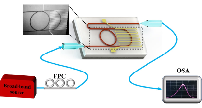
Figure 2: Schematic of the experimental setup of self-interference microring sensor launched by a broad-band laser source. FPC, fiber polarization controller, OSA, optical spectrum analyzer. An optical microscopy picture of the SIMRR device is shown in the inset of the figure, and the microheater is twisted around the upper cladding right above the sensing arm waveguide.

IV EXPERIMENTAL RESULTS AND MULTIMODE SENSING BASED ON ARTIFICIAL NEURAL NETWORK

IV.1 Raw data collection

Since the SIMRR shows a strong wavelength-dependent response, its broadband spectra contain rich frequency domain information. These transmission depths of multiple resonances extracted from the spectra were considered as the original data. They were processed by a supervised machine learning algorithm as described above. First of all, the processing models built by the BP-ANN required sufficient labeled data for training (Tcherniavskaia and Saetchnikov, 2011; Azad et al., 2016). To do so, we varied the DC voltages applied across the microheater and collected the corresponding transmission spectra of the SIMRR sensor. Here, the voltage generated by a DC source could be tuned from 0 to $4\,\mathrm{V}$ with a precision of $0.1\,\mathrm{V}$. Fig.3(a) shows the measured transmission spectra for the cases of the voltage applied across the micro-heater U=0, 1.5, 3.5 V. Here, only transmission spectra at three applied voltages are displayed so that the spectral variations are easy to be identified in the stacked figures. Within the wavelength range from $1500\,\mathrm{nm}$ to $1620\mathrm{\,nm}$, there are multiple strong and narrow resonant dips present. These dips represent resonant modes inside the SIMRR excited by the broad-band laser source. Transmission spectra at U=0 V are taken as an example to illustrate these resonant modes, which are marked by the square labels at the corresponding transmission depths. In the wavelength range, the spectra containing 49 resonant modes need to be collected for the sensing purpose. In the experiment, a variable optical attenuator was used to control the power of the laser at the level of $100\,\mathrm{\mu W}$. Then, with such low excitation power, the laser was coupled into the SIMRR through tapered lens fiber. The power level caused that the nonlinear effect in the microcavity could be neglected. Moreover, the frequency interval between these modes is enough large, and the interactions between these modes cannot occur. Besides, these transmission dips in transmission spectra were exhibited based on a plurality of different baselines. The baselines were formed mainly due to the wavelength-dependent output intensity distribution of the broad-band laser source. The other part is due to the wavelength sensitive fiber coupling efficiency in the detecting system.

Fig.3(b)-(d) separately displayed the transmission dips near $1535.2\,\mathrm{nm}$,$1569.7\,\mathrm{nm}$ and $1601.5\,\mathrm{nm}$ when the DC voltage applied across the microheater is changed from 0.3 V to 3.5 V with the step size of 0.2 V. They were indicated by the attached shadows in Fig.3(a). As shown in Fig.3(b), for the transmission dip near $1535.2\,\mathrm{nm}$, its transmission depth gets bigger with the increasing of the applied DC voltage. In Fig.3(c), the transmission depth near $1569.7\,\mathrm{nm}$ does not show a monotonous change with the change of the applied DC voltage. When the applied voltages were larger than 2.9 $\mathrm{V}$, the baselines showed a significant reduction in their intensities away from resonance. The transmission intensity fluctuation maybe stems from the interference instability inside the SIMRR. Therefore, it is unable to use the transmission dip near $1569.7\,\mathrm{nm}$ to implement dissipative sensing. However the proposed multimode sensing by BP-ANN is independent of the linear change of transmission depth, and the transmission dip near $1569.7\,\mathrm{nm}$ can be still used for multimode sensing. So the multimode sensing is robust against the choice of transmission dip. While near $1601.5\,\mathrm{nm}$ in Fig.3(d), the transmission depth gets smaller with the increasing of the applied DC voltage. Near $1535.2\,\mathrm{nm}$ or $1601.5\,\mathrm{nm}$, in the voltage range of 0 to 4 $\mathrm{V}$, the transmission depth change is not strictly linear with the increase of the applied voltage. Then the single-mode dissipative sensing could be performed in a relatively small voltage range, within which the dashed lines were marked in the figures.

Strictly speaking, the spectral shifts of all WGMs, including the changes in the resonant frequency, spectrum linewidth, and transmission depth, could be considered as the effective sensing information in nature. Nevertheless, in WGM-based sensing fields, the conventional approaches mainly focus on measuring the spectral change of single resonance. The single information channel scheme wastes a lot of sensing information from the other resonances. It is well known that the sensing model can give more accurate results with the help of multi-sensor fusion technology (Khaleghi et al., 2013). The sensor fusion is the ability to bring together inputs from a set of heterogeneous or homogeneous sensors and history values of sensor data to form a single model (Hall and Llinas, 1997; Dong et al., 2009). The sensor fusion technology is based on the measurement results by multiple sensors. The studies demonstrate that the resolution of the target parameter by this optimal fusing process is better than a single sensor’s measurement (Rao, 1998). In the case of SIMRR based sensor, the spectral shifts from multiple resonances can be regarded as multiple independent measurements by multiple sensors. The conventional single-mode dissipative sensing can be considered as the measurement by a single sensor. If these multimode sensing information are fused effectively, the multimode sensing method must outperform the best single sensor (single mode dissipative sensing).

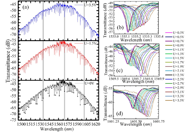
Figure 3: (a) With the micro-heater driven by various DC voltages (U=0, 1.5, 3.5 V), the experimentally measured transmission spectra of the SIMRR sensor excited by a broadband laser source, and the transmission dips near $1535.2\,\mathrm{nm}$, $1569.7\,\mathrm{nm}$ and $1601.5\,\mathrm{nm}$ are indicated by the shadows. When the DC voltages applied across the micro-heater is changed from 0.3 V to 3.5 V with the step size of 0.2 V, the experimental transmission spectra near $1535.2\,\mathrm{nm}$ (b), $1569.7\,\mathrm{nm}$ (c), and $1601.5\,\mathrm{nm}$ (d).

IV.2 Cross-validation based on the artificial network

Subsequently, the BP-ANN was successfully applied for fusing the multimode sensing information. Fig.4(a) displays a BP-ANN based signal processing procedure for the proposed multimode sensing in Section 2. In the experimental works, the BP-ANN was built to accurately estimate the voltage applied across the microheater. First, it is necessary to prepare the training set before the measurement process is started. As the sensor was used in practice, the test set was obtained by collecting a group of transmission depths within the wavelength range. It was noted that the data with unknown output voltage (unlabeled) were independent of the ones used for training, and the same data was not shared between the training set and the test set. The training set was standardized. Its data normalization could save training time and improve BP-ANN’s performance. The BP-ANN was then trained based on the training set (labeled), resulting in the development of a prediction model. Before the prediction model was validated with the test set, the test set was processed with the same standardization as the training set for scaling.

Based on the experimental results, the original data sample consists of pairs of an input vector (a group of transmission depths) and the corresponding setting voltage. If the original data sample is used as a training dataset, the voltage is commonly denoted as the target (or label). If it is selected as a test dataset, the voltage is used to compare with the result by the BP-ANN. The supervised machine learning models were developed through the K-fold cross-validation (CV) (Imamura et al., 2019). The schematic illustration of the K-fold CV is displayed in Fig.4(b). In the K-fold CV, the original data samples are randomly partitioned into K subsamples. Of the K subsamples, a single subsample is selected as the test set for validating the model, and the remaining K-1 subsamples are implemented as the training set. In this research, the training and test sets were selected from the original data samples according to the above cross-validation. Under a selection of training and test sets, the estimate process is executed by the BP-ANN. A detailed account of the BP-ANN procedure to perform the SIMRR multimode sensing can be found in Ref. (Hu et al., 2020). Due to random weight initialization in the BP-ANN before training, the output result by the BP-ANN fluctuates when it is operated each time. Here, the estimate process by the BP-ANN was repeatedly carried out n times, because its output accuracy could be improved by averaging n times estimate results. To calculate the MSE of the multimode sensing, the CV process was repeated K times (the folds), where each of the K subsamples is used exactly once as the test set. We calculated the mean square errors (MSE) between K desired output voltages and the K results from the folds, and the value is considered as the MSE of the multimode sensing. In the studies, there are 41 voltage values present when the voltage applied across the micro-heater is adjusted from 0 to 4 $\mathrm{V}$ with the step size of 0.1 $\mathrm{V}$. Then, the number of original data samples is 41, and the CV approach is taken from 41 sub-samples (41-fold). All data samples are used for training and testing, and each data sample is used for validation exactly once. Such measurement process could be made without loss of generality, and it is also an appropriate selection for objective error estimates of the multimode sensing.

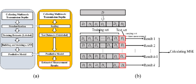
Figure 4: (a) A BP-ANN based signal processing procedure for the proposed multimode sensing. (b) Illustration of the K-fold cross-validation (CV).

IV.3 Results and discussion

As shown in Fig.5(a)-(b), the influence of related parameters on measurement results, such as learning rate, number of neurons in the hidden layer, number of repeated estimates by the BP-ANN, and training goal error, were studied to optimize the sensor performance. The initial parameter values were set as follows: the node number of 10 in the hidden layer, the training goal error of $1\times 10^{-6}$, and the number of repeated estimates of 100. Fig.5 shows the MSE versus the learning rate, and an optimal learning rate value was selected as 0.007 with the minimum MSE. Similarly, the number of neurons in the hidden layer, the number of repeated measurements, and training goal error were successively optimized, and the final parameters are selected as the node number of 5 in the hidden layer, the training goal error of $1\times 10^{-12}$, and the number of repeated measurements of 60.

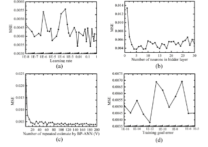
Figure 5: Influence of the network parameters on its measurement results, MSE versus (a) learning rate, (b) number of neurons in the hidden layer, (c) number of repeated estimate by the BP-ANN, and (d) training goal error.

With above-mentioned CV method, results by the BP-ANN were compared with actual reference values in Fig.6(a)-(d). We tested our method by seeding the BP-ANN with partial experimental data, i.e. with the number of resonances. Comparing the estimated values of the voltage and their corresponding experimental values, the precision increases with the number of resonances. There are few measurement errors between measurement results and their actual experimental values, except at the first and last two test indexes. At several edge test indexes, large measurement errors often occur because of the poor generalization ability of the trained BP-ANN. To evaluate the multimode sensing’s performance fairly, four edge test indexes were removed from the voltage measurement range. The MSE by the BP-ANN was averaged over all the test indexes except four edge test indexes. As the numbers of applied resonances in the proposed multimode sensing are 1, 10, 30, and 49, the values of their MSE are 0.1377, 0.093, 0.035, and $3.9\times 10^{-3}$, respectively, as shown in Fig.6(e). It is proved that the sensitivity is improved when more information inquired by the multimode sensing method.

The corresponding MSE versus the voltage was also displayed in Fig.6 (d). In the case, as the voltage applied across the microheater was adjusted from 0.0 to 4.0 $\mathrm{V}$ with the step size 0.1 $\mathrm{V}$, these original samples were numbered as test indexes from 1 to 41. When 49 resonances in Fig.3(a) is used in the multimode sensing, the value of the MSE is $3.9\times 10^{-3}$. For the multimode sensing scheme using the BP-ANN, the root-mean-square error (RMSE) is approximately equal to its limit of detection (LOD) (Hu et al., 2020). Then, the LOD of the multimode sensing is 0.062$\,\mathrm{V}$. As a comparison, the single-mode dissipative sensing was also implemented by measuring the change in the transmission depth of a single resonance. The detailed derivation of its LOD was provided in Appendix A. The LOD of the single-mode dissipative sensing near $1535.2\,\mathrm{nm}$ and $1601.5\,\mathrm{nm}$ are $0.15\,\mathrm{V}$ and $0.293\,\mathrm{V}$, respectively. The LOD achieves the optimal value for sensing near $1535.2\,\mathrm{nm}$, in comparison with the LOD values at other transmission dips. The optimal LOD of single-mode sensing is at least 2.4 times greater than that of the multimode sensing. Moreover, the multimode sensing can achieve the lower LOD within the broad voltage range of $0.2\,\mathrm{V}\leqslant U\leqslant 3.8\,\mathrm{V}$. Therefore, the experimental results proved that the performance of the multimode sensing method is superior to that of the single mode sensing.

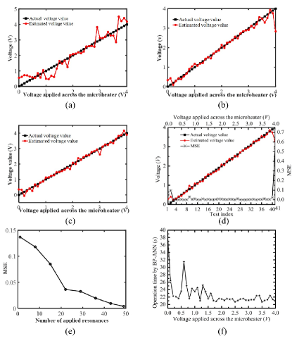
Figure 6: When the numbers of applied resonances in the sensing are 1 (a), 10 (b) and 30 (c) comparison between the estimated values of the voltage and their corresponding actual values. (d) With the number of applied resonances $n=49$, comparison between the estimated values of the voltage and their corresponding actual values versus voltage applied across the microheater, and MSE versus voltage applied across the microheater. (e) MSE versus the number of applied resonances. (f) Operation time by the BP-ANN versus voltage applied across the microheater.

The multimode SIMRR sensor’s time resolution was essentially set by the response time of the SIMRR, or roughly the SIMRR photon lifetime. In the detecting system, the scanning time by the OSA limited the time resolution of such measurements to a few seconds. When the BP-network is operated on a personal computer with Intel Core i5 2.3 GHz CPU and 8 GB memory, the operation time by the BP-ANN versus voltage applied across the microheater is displayed in Fig.6(f), where the measurement process by the BP-ANN is repeatedly performed 60 times. The average operation time of the BP-ANN is about 22.72 seconds. When the BP-ANN algorithm was run on a computer with Intel Core i7 3.7 GHz CPU and 16 GB memory, the averaged operation time was shortened to 3.78 seconds. Therefore, our approach promises the real time sensing applications with low LOD, where the experimental data acquisition time is also on the order of seconds. The ultimate operation time of our method is restricted by algorithm. In practice, two approaches can be taken to employ supervised machine learning algorithm with an even shorter time in the future. One approach is to adopt advanced fusion algorithm (deep neural networks) to accelerate operation and shorten the training time. The second approach is to transmit a big multimode sensing data to the cloud server via the 5G network, which is used to execute the algorithm with faster speed. In such a way, it is possible to realize real-time measurement performed on the multimode SIMRR sensor with low LOD.

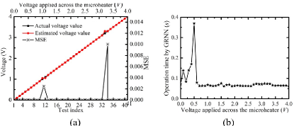
Figure 7: All the intensity samples in the spectra at $1500\thinspace\mathrm{nm}\leq\lambda\leq 1620\thinspace\mathrm{nm}$ are used to form the original data, and the GRNN algorithm is adopted to develop the predictive model. (a) The comparison between the estimated values of the voltage and their corresponding actual values versus voltage applied across the microheater, and MSE versus voltage applied across the microheater. (b) Operation time by the GRNN versus voltage applied across the microheater.

In the end, the BP-ANN was replaced with the general regression neural network (GRNN) to develop the predictive model. The GRNN has an excellent nonlinear approximation performances under small-sample data-set or unstable data (Rooki, 2016). The GRNN consists of an input layer, a hidden layer and an output layer where there is one hidden neuron for each training pattern in hidden layer. The GRNN is a one-pass learning algorithm with a highly parallel structure, and the smoothing factor is the only free parameter in GRNN. The multimode sensing informations are further expanded as the complete spectra signal, where the original sensing informations can never be lost in the frequency domain. All the intensity samples in the spectra at $1500\thinspace\mathrm{nm}\leq\lambda\leq 1620\thinspace\mathrm{nm}$ were used to form the original data, including the training and test sets. The CV method was also applied in the case. Because the output result by the GRNN fluctuates slightly when it is operated each time. Therefore, it is unnecessary to perform multiple estimates for each test voltage, and the GRNN was operated only once. With the optimized smoothing factor value of 1.3, the measurement outputs are shown in Fig.7 (a). It is observed that we get the very accurate results except that there are few errors in two test indices. The value of MSE is $1.02\times 10^{-4}$, and its LOD is close to 0.01$\,\mathrm{V}$. The optimal LOD of single-mode sensing is almost 15 times greater than that of the multimode sensing by the GRNN. The reason is that all the intensity samples in the transmission dips contain complete sensing information, and their participation in the fusion algorithm significantly enhance the performance. In addition, Fig.7(b) displays the operation time by the GRNN versus voltage applied across the microheater. The averaged operation time was shortened to 0.0808 second (a computer with Intel Core i7 3.7 GHz CPU and 16 GB memory).

In our previous research, theoretical studies proved that the LOD of the multimode sensing is more than two orders of magnitude lower than that of the single mode sensing (Hu et al., 2020). In the experiment, the LOD of the multimode sensing can be further improved by increasing the number of the training set. The estimation accuracy by the BP-ANN partly depends on the number of the training set (Hu et al., 2020). In the experiments, limited by the resolution of the voltage (0.1 $\mathrm{V}$), only 40 samples appear in the training set (one-sample test) with the voltage varied from 0 to 4 $\mathrm{V}$. Therefore, if the voltage resolution is sufficient, the training set can be constructed with enough number of samples, and the measurement accuracy by the ANN can exhibit a remarkable enhancement.

V Conclusions

In conclusion, a universal multimode sensing method has been experimentally demonstrated based on the SIMRR on a silicon nitride photonic chip. The detecting system is launched by a broad-band laser source, and the transmission depths of multiple resonances are extracted from the collected spectra as effective sensing features and merged by a BP-ANN. Compared with the single-mode dissipative sensing, the proposed SIMRR multimode sensing provides the following advantages: (i) The BP-ANN is applied to realize the nonlinear mapping relationship between a group of transmission depths and the target parameter to be detected. Hence, the measurement range is no longer restricted by the linear operation and can be expanded greatly. (ii) The multimode sensing information is fused fully by using the BP-ANN, and the LOD can be reduced considerably. (iii) In future application, for the detecting system excited by a broadband laser source, only a charged coupled device (CCD) can be used to acquire directly cavity mode intensities in combination to a designed reflection grating. (iv) More importantly, with abundant multimode sensing data, the multimode SIMRR sensing method promises multi-parameter sensing applications (Hu et al., 2020). This will bring benefits to reduce the detection cost. The SIMRR-based multimode sensing should thus provide a powerful platform to realize a simple, robust, and high-sensitive sensing scheme with low detecting cost.

Funding

The work was supported by National Key Research and Design program (2016YFA0301300); the National Natural Science Foundation of China (NSFC) (60907032, 61675183 and 61675184); Zhejiang Provincial Natural Science Foundation of China under Grant No.LY20F050009; Open Fund of the State Key Laboratory of Advanced Optical Communication Systems and Networks, China (2020GZKF013).

Disclosures

The authors declare no conflicts of interest.

Appendix A - Computation of the limit of detection of single mode dissipative sensing in the experiment

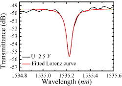
Figure A.1: At $U=2.5\,\mathrm{V}$, the experimental transmission spectra and its fitted Lorentz lineshape near $1535.2\,\mathrm{nm}$, which are indicated by the black and red solid lines, respectively.

The transmission depth change near $1535.2\,\mathrm{nm}$ was used to perform the single mode dissipative sensing, and Fig.A.1 shows the experimental transmission dip at $U=2.5\,\mathrm{V}$. They were fitted by a Lorentz lineshape curve, which can be described by the following expression,

$$I=I_{0}+\frac{2A}{\pi}\frac{\Gamma}{4(\lambda-\lambda_{0})^{2}+\Gamma^{2}}$$ (A.1)

where $I_{0}=-49.394\,\mathrm{dB},$$\lambda_{0}=1535.223\,\mathrm{nm},$$\Gamma=0.0594\,\mathrm{nm},$ and $A=-0.579\,\mathrm{dB}.$ The amplitude noises are the difference between the experimental transmission spectra and its fitted Lorentz lineshape (White and Fan, 2008; Ghasemi et al., 2014). Assuming that the amplitude noise follows a Gaussian distribution, its standard deviation $\sigma$ was approximately equal to $0.2085$$\,\mathrm{dB}$. The LOD of the single- mode dissipative sensing can be written as,

$$LOD=\frac{\sigma}{S_{I}}$$ (A.2)

where $S_{I}$ denotes the single mode dissipative sensitivity. Fig.3(b) shows the experimental transmission dip near $1535.2\,\mathrm{nm}$ as the applied voltage was changed. The single-mode dissipative sensing was realized by measuring the transmission depth changes with different sensitivities ($S_{I}$). Aided by the dashed line marked in Fig.3(b), the averaged sensitivity is about $1.389\,\mathrm{dB/V}$ at $1.7\,\mathrm{V}\leqslant U\leqslant 3.5\,\mathrm{V}$. Hence, the LOD of the single-mode dissipative sensing is 0.15$\,\mathrm{V}$ according to Eq. (2). In the same way, for the transmission dips in Fig.3 (d), its LOD value is about $0.293\,\mathrm{V}$, where the noise standard deviation $\sigma$ is $0.3779$$\,\mathrm{dB}$, and its average sensitivity is 1.293$\,\mathrm{dB/V}$ at $1.3\,\mathrm{V}\leqslant U\leqslant 3.3\,\mathrm{V}$.

References

- Jiang et al. (2020) X. Jiang, A. J. Qavi, S. H. Huang, and L. Yang, Matter 3, 371 (2020).
- Qian et al. (2018) Y. Qian, Y. Zhao, Q.-l. Wu, and Y. Yang, Sensors and Actuators B: Chemical 260, 86 (2018).
- Xue et al. (2019) T. Xue, W. Liang, Y. Li, Y. Sun, Y. Xiang, Y. Zhang, Z. Dai, Y. Duo, L. Wu, K. Qi, et al., Nature communications 10, 1 (2019).
- Song (2019) Q. Song, Sci. China Phys. Mech. Astron 62, 074231 (2019).
- Zou et al. (2012) C. Zou, C. Dong, J. Cui, F. Sun, Y. Yang, X. Wu, Z. Han, and G. Guo, SCIENTIA SINICA Physica, Mechanica & Astronomica 42, 1155 (2012).
- Chen et al. (2017) W. Chen, Ş. K. Özdemir, G. Zhao, J. Wiersig, and L. Yang, Nature 548, 192 (2017).
- Zhang et al. (2017) X. Zhang, Y. Yang, H. Bai, J. Wang, M. Yan, H. Xiao, and T. Wang, Photonics Research 5, 516 (2017).
- Qin et al. (2019) G.-Q. Qin, M. Wang, J.-W. Wen, D. Ruan, and G.-L. Long, Photonics Research 7, 1440 (2019).
- Foreman et al. (2015) M. R. Foreman, J. D. Swaim, and F. Vollmer, Advances in optics and photonics 7, 168 (2015).
- Zhang et al. (2018) Y.-n. Zhang, T. Zhou, B. Han, A. Zhang, and Y. Zhao, Nanoscale 10, 13832 (2018).
- Zhi et al. (2017) Y. Zhi, X.-C. Yu, Q. Gong, L. Yang, and Y.-F. Xiao, Advanced Materials 29, 1604920 (2017).
- La Notte et al. (2014) M. La Notte, B. Troia, T. Muciaccia, C. E. Campanella, F. De Leonardis, and V. Passaro, Sensors 14, 4831 (2014).
- Khaleghi et al. (2013) B. Khaleghi, A. Khamis, F. O. Karray, and S. N. Razavi, Information fusion 14, 28 (2013).
- Zhu et al. (2010) J. Zhu, S. K. Ozdemir, Y.-F. Xiao, L. Li, L. He, D.-R. Chen, and L. Yang, Nature photonics 4, 46 (2010).
- Zhu et al. (2011) J. Zhu, Ş. K. Özdemir, L. He, D.-R. Chen, and L. Yang, Optics express 19, 16195 (2011).
- Kim et al. (2012) W. Kim, S. K. Ozdemir, J. Zhu, F. Monifi, C. Coban, and L. Yang, Optics Express 20, 29426 (2012).
- Yi et al. (2010) X. Yi, Y.-F. Xiao, Y. Li, Y.-C. Liu, B.-B. Li, Z.-P. Liu, and Q. Gong, Applied Physics Letters 97, 203705 (2010).
- Mallik et al. (2018) A. K. Mallik, G. Farrell, M. Ramakrishnan, V. Kavungal, D. Liu, Q. Wu, and Y. Semenova, Optics Express 26, 31829 (2018).
- Ren et al. (2016) H. Ren, C.-L. Zou, J. Lu, L.-L. Xue, S. Guo, Y. Qin, and W. Hu, IEEE Photonics Technology Letters 28, 1469 (2016).
- Ren et al. (2019) H. Ren, C.-L. Zou, J. Lu, Z. Le, Y. Qin, S. Guo, and W. Hu, JOSA B 36, 942 (2019).
- Hu et al. (2020) D. Hu, C.-l. Zou, H. Ren, J. Lu, Z. Le, Y. Qin, S. Guo, C. Dong, and W. Hu, Sensors 20, 709 (2020).
- Wan et al. (2018) S. Wan, R. Niu, H.-L. Ren, C.-L. Zou, G.-C. Guo, and C.-H. Dong, Photonics Research 6, 681 (2018).
- Feng et al. (2017) J. Feng, R. Akimoto, Q. Hao, and H. Zeng, IEEE Photonics Technology Letters 29, 771 (2017).
- Ma et al. (2019) K. Ma, Y. Zhang, H. Su, C. Yu, and J. Wang, Journal of Lightwave Technology 37, 3728 (2019).
- Yu and Fan (2011) Z. Yu and S. Fan, Optics express 19, 10029 (2011).
- Hall and Llinas (1997) D. L. Hall and J. Llinas, Proceedings of the IEEE 85, 6 (1997).
- Dong et al. (2009) J. Dong, D. Zhuang, Y. Huang, and J. Fu, Sensors 9, 7771 (2009).
- Bishop (1995) C. M. Bishop, Neural networks for pattern recognition (Oxford university press, 1995).
- Daria et al. (2020) K. Daria, S. Gregor, H. Lothar, M. Johannes, H. Andreas, L. Kerstin, F. Wolfgang, and K. Christian, Light: Science & Applications submitted. (2020).
- Jin et al. (2011) L. Jin, M. Li, and J.-J. He, Optics letters 36, 1128 (2011).
- Acharyya et al. (2019) N. Acharyya, M. Maher, and G. Kozyreff, Optics express 27, 34997 (2019).
- Tcherniavskaia and Saetchnikov (2011) E. Tcherniavskaia and V. Saetchnikov, Journal of Applied Spectroscopy 78, 457 (2011).
- Azad et al. (2016) A. K. Azad, L. Wang, N. Guo, H.-Y. Tam, and C. Lu, Optics express 24, 6769 (2016).
- Rao (1998) N. S. Rao, A fusion method that performs better than best sensor, Tech. Rep. (Oak Ridge National Lab., TN (United States), 1998).
- Imamura et al. (2019) G. Imamura, K. Shiba, G. Yoshikawa, and T. Washio, Scientific reports 9, 1 (2019).
- Rooki (2016) R. Rooki, Measurement 85, 184 (2016).
- White and Fan (2008) I. M. White and X. Fan, Optics express 16, 1020 (2008).
- Ghasemi et al. (2014) F. Ghasemi, M. Chamanzar, A. A. Eftekhar, and A. Adibi, Analyst 139, 5901 (2014).