Solving path dependent PDEs with LSTM networks and path signatures

Abstract.

Using a combination of recurrent neural networks and signature methods from the rough paths theory we design efficient algorithms for solving parametric families of path dependent partial differential equations (PPDEs) that arise in pricing and hedging of path-dependent derivatives or from use of non-Markovian model, such as rough volatility models [34]. The solutions of PPDEs are functions of time, a continuous path (the asset price history) and model parameters. As the domain of the solution is infinite dimensional many recently developed deep learning techniques for solving PDEs do not apply. Similarly as in [44], we identify the objective function used to learn the PPDE by using martingale representation theorem. As a result we can de-bias and provide confidence intervals for then neural network-based algorithm. We validate our algorithm using classical models for pricing lookback and auto-callable options and report errors for approximating both prices and hedging strategies.

1. Introduction

Deep neural networks trained with stochastic gradient descent algorithms are extremely successful in number of applications such as computer vision, natural language processing, generative models or reinforcement learning [25]. As these methods work extremely well in seemingly high-dimensional settings, it is natural to investigate their performance in solving high-dimensional PDEs. Starting with the pioneering work [28, 19], where probabilistic representation has been used to learn PDEs using neural networks, recent years have brought an influx of interest in deep PDE solvers. As a result there is now a number of efficient algorithms for solving linear and non-linear PDEs, employing probabilistic representations, that work in high dimensions [6, 8, 24, 26, 4].

The methods in [28, 19] approximate a solution to a single PDE at a single point in space. The first paper to extend the above techniques to families of parametric PDEs with approximations across the whole domain was [44]. In this paper we extend this to parametric families of path-dependent PDEs (PPDEs). Let $B\subseteq\mathbb{R}^{p},p\geq 1$ be a parameter space. Consider $F=F(t,\omega;\beta)$ satisfying

(1.1) $$\begin{split}&\bigg{[}\partial_{t}F+b\nabla_{\omega}F+\frac{1}{2}\text{tr}\left[\nabla_{\omega}^{2}F\sigma^{*}\sigma\right]-rF\bigg{]}(t,\omega;\beta)=0\,,\\ &F(T,\omega;\beta)=g(\omega;\beta)\,,\,\,\,t\in[0,T]\,,\,\,\omega\in C([0,T];\mathbb{R}^{d})\,,\,\,\beta\in B\,.\end{split}$$

Here $t\in[0,T]$, $\omega\in C([0,T];\mathbb{R}^{d})$ and $\beta\in B$ and $b,\sigma,r$ and $g$ are functions of $(t,\omega;\beta)$ which specify the problem. Notice that we are dealing with an equation in an infinite dimensional space. The derivatives $\nabla_{\omega}$ and $\nabla_{\omega}^{2}$ are derivatives on the path space $C([0,T];\mathbb{R}^{d})$, see Appendix A, introduced in [18, 14, 16] in the context of functional Itô calculus.

The Feynman–Kac theorem provides a probabilistic representation for $F$ and so Monte Carlo methods can be used to approximate $F$ for a single fixed $(t,\omega;\beta)$. Nevertheless, it is clear that approximating the PPDE solution $F$ across the whole space $[0,T]\times C([0,T];\mathbb{R}^{d})\times B$ is an extremely challenging task. A key step is efficiently encoding the information in $\omega$ in some finite dimensional structure.

Equations of the form (1.1) arise in mathematical finance with $F$ representing a price of some (path-dependent) derivative. In this context $\beta$ would be model parameters, $t$ the current time and $\omega$ a path “stopped at $t$” representing the price history of some assets. Moreover $\nabla_{\omega}F$ is an object which, in many models, gives access to a “hedging strategy” which is of key importance for risk management purposes. Having an approximation of $F$ that can be quickly evaluated for any $\beta\in B$ is essential for model calibration (see e.g. [31]).

1.1. Main contributions

The main contributions in this paper are the following:

1. We provide two methods for efficiently encoding the paths $\omega$ using long-short-term-memory (LSTM)-based deep learning methods and path-signatures to approximate the solution of a parabolic PPDE on the whole domain and parameter space.

2. We provide methods for removing bias in the approximation and a posteriori confidence intervals for then neural network-based approximation.

3. The algorithms we develop are applicable to parametric families of solutions and hence can be used for efficient model calibration from data.

4. The algorithms we develop provide approximation of $\nabla_{\omega}F$ thus providing access to the hedging strategies.

5. We test the algorithms for various models and study their relative performance. The code for our proposed methods and for the numerical experiments can be found at
   https://github.com/msabvid/Deep-PPDE.

1.2. Overview of existing methods

Let us now provide a brief overview of other methods available in the literature. As has already been mentioned, the probabilistic methods for deep PDE solvers were first explored in [28, 19] (providing solution for a single point in time and space). These methods were further extended in [9, 39, 32, 5] to build deep learning solvers for non-linear PDEs. In [44] the probabilistic methods were extended to families of parametric PDEs with approximations across the whole domain. A different (non-probabilistic) approach was adopted in [42]. There a deep neural network is directly trained to satisfy the differential operator, initial and boundary conditions. This relies on automatic differentiation to calculate the gradient of the network in terms of its input. Related algorithms are being developed in the so-called physics inspired machine learning [40] where one uses PDEs as regulariser of the neural network. See [20] for a survey of recent efforts to solve PDEs in high dimension using deep learning.

Deep Learning methods that approximate the solution of PPDEs have been studied in [41], where the authors extend the work from [42] and they use a LSTM network to include the path-dependency of the solution of the PPDE. A different approach is proposed in [34] where the authors first discretise the space to approximate a PPDE by high-dimensional classical PDE, and use deep BSDE solver approach to solve it.

Unlike the methods mentioned earlier, the algorighms in this paper can be used for parametric families of solutions of PDEs (PPDEs). Having approximation of $F(\cdot;\beta)$ for any $\beta\in B$ allows for swift calibration of models to market data (e.g options prices) since we also have access to $\nabla_{\beta}F$ using automatic differentiation. This is particularly appealing for high dimensional problems or for models for which computation of the pricing operator is costly. This line of research has been recently studied in various settings and with various datasets [31, 36, 3, 43, 29, 33, 38]. Recent work in [17, 22] use Neural SDEs to perform a data-driven model calibration i.e. without using a prior assumption on the form of the dynamics of the price process.

1.3. Outline

In Section 2 we define the notion of Path Dependent PDE, relying on Functional Itô Calculus, and we introduce the Feynman–Kac formula extended for path-dependent functionals. Section 3 develops the martingale representation of the discounted price of a path-dependent option, and how it can be used to retrieve the hedging strategy. Section 4 develops the algorithms to approximate the solution of a linear PPDE, built on the probabilistic representation of the solution of the PPDE, and the properties of the conditional expectation and the martingale representation of the discounted price. We finally provide some numerical experiments in Section 5.

1.4. Notation

We will use the following notation

• $t\wedge s=\min(t,s)$

• Let $m,d,\kappa,p,N\in\mathbb{N}$, $B\subseteq\mathbb{R}^{p}$. Let $F:[0,T]\times C([0,T],\mathbb{R}^{d})\times B\rightarrow\mathbb{R}^{m}$ such that $F(\cdot,\cdot;\beta)$ is a non-anticipative functional for all $\beta\in B$ (see Section 2 and Appendix A). We denote a neural network with weights $\theta\in\mathbb{R}^{\kappa}$ approximating $F$ as:

  $$\mathcal{R}_{\theta}[F]:[0,T]\times\mathbb{R}^{N}\times B\rightarrow\mathbb{R}^{m}$$

  where a path $\omega\in C([0,T],\mathbb{R}^{d})$ is encoded by an element of $\mathbb{R}^{N}$ (see Sections 4.1, 4.2).

• $\nabla_{\omega}F(t,\omega;\beta)$ and $\nabla_{\omega}^{2}F(t,\omega;\beta)$ are the vector and matrix denoting the first and second order path-derivatives (see Appendix A) of a non-anticipative functional. Furthermore, the space of non-anticipative functionals admitting time-derivative up to first order and path-derivative up to second order, in addition to satisfying the boundedness property of their time and path-derivatives (Appendix A) is denoted by $\mathbb{C}^{1,2}$.

• $\text{Sig}^{(n)}_{[t_{i},t_{j}]}$ denotes the path signature up to the $n$-th iterated integral of a path $(\omega_{t})_{t\in[t_{i},t_{j}]}$.

2. PPDE-SDE relationship

Appendix A provides a brief review of the notion of non-anticipative functionals and their path derivatives. In short, a non-anticipative functional $F:[0,T]\times C([0,T],\mathbb{R}^{d})\rightarrow\mathbb{R}$ does not look into the future, i.e. given $t\in[0,T]$ and two different paths $\omega,\omega^{\prime}\in C([0,T],\mathbb{R}^{d})$ such that $\omega_{s\wedge t}=\omega^{\prime}_{s\wedge t}\,\,\,\forall s\in[0,T]$, then $F(t,\omega)=F(t,\omega^{\prime})$.

The following result allows to represent the solution of a linear PPDE with terminal condition as the expected value of a random variable. Fix a probability space $(\Omega,\mathcal{F},\mathbb{P})$, and consider a continuous process $(X_{t})_{t\in[0,T]}$ given by

(2.1) $$dX_{t}^{\beta}=b(t,(X_{t\wedge s}^{\beta})_{s\in[0,T]};\beta)dt+\sigma(t,(X_{t\wedge s}^{\beta})_{s\in[0,T]};\beta)dW_{t}$$

where $b,\sigma$ are non-anticipative functionals and $(W_{t})_{t\in[0,T]}$ is a Brownian motion, and $\beta\in B\subseteq\mathbb{R}^{p}$. Furthermore, assume that $b,\sigma$ are such that the SDE admits a unique strong solution. On the other hand, let $F$ satisfy the following conditions:

1. it is regular enough admitting time derivative up to first order and path-derivatives up to second order (as defined in Appendix A).

2. it is the solution of the following linear PPDE,

   (2.2) $$\begin{split}&\bigg{[}\partial_{t}F+b\nabla_{\omega}F+\frac{1}{2}\text{tr}\left[\nabla_{\omega}^{2}F\sigma^{*}\sigma\right]-rF\bigg{]}(t,\omega;\beta)=0\,,\\ &F(T,\omega;\beta)=g(\omega;\beta)\,,\,\,\,t\in[0,T]\,,\,\,\omega\in C([0,T];\mathbb{R}^{d})\,,\,\,\beta\in B\,.\end{split}$$

Then one can establish a probabilistic representation of $F(t,\omega;\beta)$ via the Feynman-Kac formula. In the following result, we assume $\beta$ fixed, and we abuse the notation to write $F(t,\omega):=F(t,\omega;\beta)$.

Theorem 2.1 (Feynman-Kac formula for path-dependent functionals, see Th. 8.1.13 in  [2]).

Consider the functional $g:C([0,T],\mathbb{R}^{d})\rightarrow\mathbb{R}$, continuous with respect to the distance $d_{\infty}(\omega,\omega^{\prime}):=\sup_{t\in[0,T]}|\omega(t)-\omega^{\prime}(t)|$. If for every $(t,\omega)\in\left([0,T],C([0,T],\mathbb{R}^{d})\right)$ the functional $F\in\mathbb{C}^{1,2}$ verifies (2.2), then $F$ has the probabilistic representation

(2.3) $$F(t,\omega)=e^{-r(T-t)}\mathbb{E}\left[g((X_{t})_{t\in[0,T]})\bigg{|}(X_{t\wedge s})_{s\in[0,T]}=(\omega_{t\wedge s})_{s\in[0,T]}\right].$$

with $(X_{t})_{t\in[0,T]}$ given by (2.1).

A direct consequence of the Feynman–Kac formula for path-dependent functionals is that solving (2.2) is equivalent to pricing the path-dependent option with payoff at $T$ given by $g((X_{s})_{s\in[0,T]})\in L^{2}(\mathcal{F}_{T})$ where $(X_{t})_{t\geq 0}$ is the solution of (2.1) and $(\mathcal{F}_{t})_{t\geq 0}$ denotes the filtration generated by $(X_{t})_{t\geq 0}$. We will build two algorithms based on two different approaches:

1. Option pricing using the martingale representation theorem (Algorithm 3).

2. Considering the conditional expectation in  (2.3) as the orthogonal projection of $g(X_{T})$ on $\mathcal{L}^{2}(\mathcal{F}_{t})$ where $(\mathcal{F}_{t})_{t\geq 0}$ is the filtration generated by $(X_{t})_{t\geq 0}$ (Algorithm 2).

3. Option pricing via Martingale Representation Theorem

In this section we assume constant interest rate and a complete market but the results readily extend to the case of stochastic interest rates and incomplete markets.

Let $(\Omega,\mathcal{F},\mathbb{Q})$ be a probability space where $\mathbb{Q}$ is the risk-neutral measure. Consider an $\mathbb{R}^{d}$-valued Wiener process $W=(W^{j})_{j=1}^{d}=((W^{j}_{t})_{t\geq 0})_{j=1}^{d}$. We will use $(\mathcal{F}^{W}_{t})_{t\geq 0}$ to denote the filtration generated by $W$. Consider an $D\subseteq\mathbb{R}^{d}$-valued, continuous, stochastic process $X=(X^{i})_{i=1}^{d}=((X^{i}_{t})_{t\geq 0})_{i=1}^{d}$ that is adapted to $(\mathcal{F}^{W}_{t})_{t\geq 0}$. We will use $(\mathcal{F}_{t})_{t\geq 0}$ to denote the filtration generated by $X$.

We recall that we denote by $\beta\in B\subseteq\mathbb{R}^{p}$ the family of parameters of the dynamics of the underlying asset (for instance, in the Black–Scholes model with fixed risk-free rate, $\beta$ denotes the volatility). Let $g:C([0,T],\mathbb{R}^{d})\times B\to\mathbb{R}$ such that $g(\cdot,\beta)$ is a measurable function for each $\beta\in B\subseteq\mathbb{R}^{p}$. We shall consider contingent claims of the form $g((X_{s}^{\beta})_{s\in[0,T]};\beta)$. This means that we can consider path-dependent derivatives. Finally, let $r$ be some risk-free rate, and consider, for each $\beta$, the SDE

$$dX_{t}^{\beta}=rX_{t}^{\beta}dt+\sigma(t,(X_{s\wedge t}^{\beta})_{s\in[0,T]};\beta)dW_{t}.$$

We immediately see that $\bar{X}_{t}^{\beta}=(e^{-rt}X_{t}^{\beta})_{t\in[0,T]}$ is a (local) martingale.

In order to price an option at time $t$ with payoff $g$, under appropriate assumptions on $g$ and $\sigma$, the random variable

$$M_{t}^{\beta}:=\mathbb{E}\left[e^{-rT}g((X_{s}^{\beta})_{s\in[0,T]};\beta)\bigg{|}\mathcal{F}_{t}^{\beta}\right]$$

is square-integrable. $M_{T}^{\beta}=e^{-rT}g((X_{s}^{\beta})_{s\in[0,T]})$ is the discounted payoff at $T$. Hence $F(t,(X_{t\wedge s}^{\beta})_{s\in[0,T]};\beta)=e^{rt}M_{t}^{\beta}$ is the fair price of the option with payoff $g$ at time $t$. By the Martingale representation theorem, for each $\beta$ there exists a unique $\mathcal{F}_{t}$-adapted process $Z_{s}^{\beta}$ with $\mathbb{E}\left[\int_{0}^{T}(Z_{s}^{\beta})^{2}ds\right]<\infty$ such that

(3.1) $$M_{T}^{\beta}=\mathbb{E}[M_{T}^{\beta}|\mathcal{F}_{0}]+\int_{0}^{T}Z_{s}^{\beta}dW_{s}.$$

In order to retrieve the real hedging strategy from the martingale representation, it is necessary to apply the Itô formula for non-anticipative functionals of a continuous semimartingale, see [18, 15]:

Proposition 3.1.

. Let $X$ be a continuous semimartingale defined on $(\Omega,\mathcal{F},\mathbb{Q})$. Then, for any non-anticipative functional $F\in\mathbb{C}^{(1,2)}$ (introduced in Section 1.4) and any $t\in[0,T]$, we have

(3.2) $$\begin{split}dF(t,(X_{s\wedge t})_{s\in[0,T]})=&\partial_{t}F(t,(X_{s\wedge t})_{s\in[0,T]})dt+\nabla_{\omega}F(t,(X_{s\wedge t})_{s\in[0,T]})dX_{t}\\ &+\frac{1}{2}\text{tr}\left((\nabla_{\omega}^{2}F(t,(X_{s\wedge t})_{s\in[0,T]}))dX_{t}dX_{t}\right).\end{split}$$

Let $\bar{F}_{t}:=e^{-rt}F(t,(X_{t\wedge s}^{\beta})_{s\in[0,T]};\beta)$ be the discounted price of the option with payoff $g$ at time $t$. Then, using (3.2),

(3.3) $$d\bar{F}_{t}=\left(-rF+\partial_{t}F+\frac{1}{2}\text{tr}(\nabla_{\omega}^{2}F\sigma^{*}\sigma)+rX_{t}\nabla_{\omega}F\right)e^{-rt}dt+\nabla_{\omega}F\cdot e^{-rt}\sigma dW_{t}\,.$$

Moreover, $\bar{F}_{t}$ is the value of the discounted portfolio at $t$ (since the market is complete) thus the coefficient of $dt$ in (3.3) is 0. Noting that $d\bar{X}_{t}^{\beta}=e^{-rt}\sigma(t,(X_{t\wedge s}^{\beta})_{s\in[0,T]};\beta)dW_{t}$, we get

$$d\bar{F}_{t}=\nabla_{\omega}Fd\bar{X}_{t}.$$

Hence after replacing in (3.1) one can retrieve the hedging strategy

(3.4) $$M_{t}^{\beta}=\mathbb{E}[M_{t}^{\beta}|\mathcal{F}_{0}]+\int_{0}^{t}\nabla_{\omega}F\,d\bar{X}_{s}^{\beta},\quad M_{T}^{\beta}=e^{-rT}g((X_{s}^{\beta})_{s\in[0,T]};\beta)\,.$$

Both $M_{t}^{\beta}$ and the stochastic integral in (3.4) are martingales. This will be used in Section 4.4 to build a learning task to solve the BSDE (3.1) to jointly approximate the fair price of the option $F$, and the hedging strategy $\nabla_{\omega}F$.

4. Deep PPDE solver Methodology

In this section we present the PPDE solver methodology consisting on the data simulation scheme (Section 4.1). We briefly define the signature of a path, that we will use as a path feature extractor (Section 4.2). We describe two optimisation tasks to approximate the price of path-dependent derivatives, relying on conditional expectation properties (Section 4.3), and on the martingale representation of the discounted price (Section 4.4). We present the learning scheme leveraging the learning methods, the different deep network architectures considered, and the path signatures (Section 4.6). Finally, we present the evaluation metrics used in the numerical experiments (Section 4.7).

4.1. Data simulation scheme

We consider the SDE with path-dependent coefficients

(4.1) $$dX_{t}^{\beta}=rX_{t}^{\beta}dt+\sigma((X_{t\wedge s}^{\beta})_{s\in[0,T]};\beta)dW_{t},\,\,\,t\in[0,T]\,,\,\,\,X(0)=x_{0},$$

and the path-dependent payoff, $g:C([0,T],\mathbb{R}^{d})\times B\to\mathbb{R}$. We will consider two different time discretisations.

1. First, a fine time discretisation $\pi^{f}:=\{0=t_{0}^{f}<t_{1}^{f}<\ldots<t_{N}^{f}=T\}$ used by the numerical SDE solver to sample paths from (4.1).

2. We consider a second, coarser, time discretisation $\pi^{c}:=\{0=t_{0}^{c}<t_{1}^{c}<\ldots<t_{N}^{c}=T\}\subseteq\pi^{f}$ on which we learn the deep learning approximation of the price of the option.

Furthermore, we fix the distribution of $\beta\in B\subseteq\mathbb{R}^{p}$. We will denote the discretisation of $(X_{t}^{\beta})_{t\in[0,T]}$ in $\pi^{f}$ using Euler scheme as $(X^{\beta,\pi^{f}}_{t})_{t\in\pi^{f}}$

4.2. Path signatures as feature extractors of paths

The input to $\mathcal{R}_{\theta}[F]$ is a discretisation of elements of $[0,T]\times C([0,T],\mathbb{R}^{d})\times B$. given by the numerical approximation from the SDE solver, $(x_{t}^{\beta,\pi^{f}})_{t\in\pi^{f}}\in\mathbb{R}^{N}$. If $\pi^{f}$ is a fine partition of $[0,T]$, then the input to $\mathcal{R}_{\theta}[F]$ will be high dimensional. We explore two alternatives to avoid feeding the whole path to the neural network. The first naive approach is feeding the path generated with the SDE solver on $\pi^{f}$ but evaluated on the coarser time discretisation $(x_{t}^{\beta,\pi^{f}})_{t\in\pi^{c}}$. In such approach the information carried by the path in the the points of $\pi^{f}$ that are not in $\pi^{c}$ is lost. Alternatively, we use path signatures to capture a description of the path on $\pi^{f}$, and provide it as an input to the neural network.

We refer the reader to Appendix B and the references therein for supplementary material on path signatures. Let $T((\mathbb{R}^{d})):=\bigoplus_{k=0}^{\infty}(\mathbb{R}^{d})^{\otimes k}$ be a tensor algebra space. Then, the signature of $X:[a,b]\rightarrow\mathbb{R}^{d}$ is an element of the tensor algebra $T((\mathbb{R}^{d}))$,

$$\text{Sig}_{a,b}(X)=(1,S(X)_{a,b}^{(1)},S(X)_{a,b}^{(2)},\ldots)\in T((\mathbb{R}^{d})).$$

where

$$S(X)_{a,t}^{(k)}=\int_{a<t_{1}<t_{2}<\ldots<t_{k}<t}dX_{t_{1}}\otimes\ldots\otimes dX_{t_{l}}\in T^{k}(\mathbb{R}^{d})$$

In short, the signature of a path determines the path essentially uniquely (up to time reparametrisations), providing top-down description of the path: low order terms of the signature capture global properties of the path (for instance $S(X)_{a,b}^{(1)}$ provides the change of each of the path coordinates between $a$ and $b$), whereas higher order terms give information on the local structure of the path.

Let $(x_{t}^{\beta,\pi^{f}})_{t\in\pi^{f}}$ be the discretisation of a path on $\pi^{f}$ generated by the SDE solver. Then we encode it as stream of signatures as follows

(4.2) $$(y_{t_{k}}^{\beta,\pi^{f}})_{t_{k}\in\pi^{c}}:=\left(\text{Sig}_{[t_{k},t_{k+1}]}^{(n)}(x_{t}^{\beta,\pi^{f}})_{t\in\pi^{f}}\right)_{t_{k}\in\pi^{c}},$$

i.e. such that each element of $(y_{t_{k}}^{\beta,\pi^{f}})_{t_{k}\in\pi^{c}}$ is the signature of $(x_{t}^{\beta,\pi^{f}})_{t\in\pi^{f}}$ between consecutive steps of $\pi^{c}$.

4.3. Learning conditional expectation as orthogonal projection

The following theorem recalls a well known property of conditional expectations:

Theorem 4.1.

Let $X\in\mathcal{L}^{2}(\mathcal{F})$. Let $\mathcal{G}\subset\mathcal{F}$ be a sub $\sigma$-algebra. There exists a random variable $Y\in\mathcal{L}^{2}(\mathcal{G})$ such that

(4.3) $$\mathbb{E}[|X-Y|^{2}]=\inf_{\eta\in\mathcal{L}^{2}(\mathcal{G})}\mathbb{E}[|X-\eta|^{2}].$$

The minimiser, $Y$, is unique and is given by $Y=\mathbb{E}[X|\mathcal{G}]$.

The theorem tells us that the conditional expectation is an orthogonal projection of a random variable $X$ onto $\mathcal{L}^{2}(\mathcal{G})$. To formulate the learning task in our problem, we replace $X$ in (4.3) by $e^{-r(T-t)}g((X_{s}^{\beta})_{s\in[0,T]};\beta)$. We also replace $\mathcal{G}$ by $\mathcal{F}^{\beta}_{t}$, and $\mathcal{F}$ by $\mathcal{F}_{T}^{\beta}$. Then by Theorem 4.1

$$\begin{split}F(t,(X_{s}^{\beta})_{s\in[0,T]};\beta)&=\mathbb{E}[e^{-r(T-t)}g((X^{\beta}_{s})_{s\in[0,T]};\beta)|\mathcal{F}_{t}^{\beta}]\\ \ &=\arg\inf_{\eta\in\mathcal{L}^{2}\left(\mathcal{F}_{t}\right)}\mathbb{E}[|e^{-r(T-t)}g((X_{s}^{\beta})_{s\in[0,T]};\beta)-\eta|^{2}]\end{split}$$

By the Doob–Dynkin Lemma [13, Th. 1.3.12] we know that every $\eta\in L^{2}(\mathcal{F}_{t}^{\beta})$ can be expressed as $\eta=h_{t}((X^{\beta}_{s\wedge t})_{s\in[0,T]})$ for some appropriate measurable $h_{t}$. For the practical algorithm we restrict the search for the function $h_{t}$ to the class that can be expressed as deep neural networks.

We then consider deep network approximations of the price of the path-dependent option at any time $t_{k}^{c}$ in the time partition $\pi^{c}$, either by directly using the path evaluated at each time step of $\pi^{c}$ or by using the stream of signatures (4.2):

(4.4) $$\text{i)}\,\,(\mathcal{X}_{t}^{\beta,\pi^{f}})_{t\in\pi^{c}}:=(x_{t}^{\beta,\pi^{f}})_{t\in\pi^{c}}\qquad\text{or ii)}\,\,(\mathcal{X}_{t}^{\beta,\pi^{f}})_{t\in\pi^{c}}:=(y_{t}^{\beta,\pi^{f}})_{t\in\pi^{c}}$$

and set the learning task as

(4.5) $$\theta^{*}=\operatorname*{arg\,min}_{\theta}\mathbb{E}_{\beta}\left[\mathbb{E}_{(X_{t}^{\beta,\pi^{f}})_{t\in\pi^{f}}}\left[\sum_{k=0}^{N}\left(e^{-r(T-t_{k})}g((X_{t}^{\beta,\pi^{f}})_{t\in\pi^{f}};\beta)-\mathcal{R}_{\theta}[F](t_{k},(\mathcal{X}_{t}^{\beta,\pi^{f}})_{t\in\pi^{c}},\beta)\right)^{2}\right]\right]\,.$$

We observe that the inner expectation in (4.5) is taken across all paths generated using the numerical SDE solver on (4.1) on $\pi^{f}$ for a fixed $\beta$ and it allows to price an option for such $\beta$. The outer expectation is taken on $\beta$ for which the distribution is fixed (as specified in the data simulation scheme), thus allowing to find the optimal neural network weights $\theta^{*}$ to price the parametric family of options.

Algorithm 1 Data simulation

  Initialisation: $N_{\text{trn}}\in\mathbb{N}$ large, distribution of $\beta$.

  for $i:1:N_{\text{trn}}$ do

      Generate training paths $(x_{t}^{\beta,\pi^{f},i})_{t\in\pi^{f}}$ using the numerical SDE solver on  (4.1) and sampling from the distribution of $\beta$ .

  end for

  if Network input is path discretisation at $\pi^{c}$ then

     $(\mathcal{X}_{t}^{\beta,\pi^{f},i})_{t\in\pi^{c}}$ := $(x_{t}^{\beta,\pi^{f},i})_{t\in\pi^{c}}$

  else

     $(\mathcal{X}_{t_{k}}^{\beta,\pi^{f},i})_{t_{k}\in\pi^{c}}:=\left(\text{Sig}_{[t_{k},t_{k+1}]}^{(n)}(X_{t}^{\beta,\pi^{f},i})_{t\in\pi^{f}}\right)_{t_{k}\in\pi^{c}}$ i.e. $\mathcal{X}$ is the process of signatures of the path between consecutive time-points of $\pi^{c}$.

  end if

  return  $(x_{t}^{\beta,\pi^{f},i})_{t\in\pi^{c}},(\mathcal{X}_{t_{k}}^{\beta,\pi^{f},i})_{t_{k}\in\pi^{c}}$ for $i=1,\ldots,N_{\text{trn}}$.

Algorithm 2 Learning orthogonal projection

  Initialisation: Weights $\theta$ of networks $\mathcal{R}[F]_{\theta}$, $N_{\text{trn}}\in\mathbb{N}$ large, distribution of $\beta$.

  Use SGD to find $\theta^{*}$, where in each iteration of SGD we generate a batch of paths (or a batch of stream of signatures) using Algorithm 1.

$$\theta^{*}={\operatorname*{arg\,min}_{\theta}}\,\,\,\mathbb{E}^{\mathbb{Q}^{N_{\text{trn}}}}\left[\sum_{k=0}^{N_{\text{steps}}-1}\left(e^{-r(T-t_{k})}g((X_{t}^{\beta,\pi^{f}})_{t\in\pi^{f}})-\mathcal{R}[F]_{\theta}(t_{k},(\mathcal{X}_{t}^{\beta,\pi^{f}})_{t\in\pi^{c}},\beta)\right)^{2}\right]$$

where $\mathbb{E}^{\mathbb{Q}^{N_{\text{trn}}}}$ denotes the empirical mean.

  return  $\theta^{*}$.

4.4. Learning martingale representation of the option price

From Section 3, for fixed $\beta$ the discounted price of the option with payoff $g$ is given by

(4.6) $$M_{T}^{\beta}=\mathbb{E}[M_{T}^{\beta}|\mathcal{F}_{0}]+\int_{0}^{T}\nabla_{\omega}F\,d\bar{X}_{s}^{\beta}.$$

Since both $(M_{t}^{\beta})_{t\in[0,T]}$ and the stochastic integral are martingales, after taking expectations conditioned on $\mathcal{F}_{s}^{\beta},\mathcal{F}_{t}^{\beta}$ on both sides for $s<t\leq T$ one gets

(4.7) $$M_{t}^{\beta}=M_{s}^{\beta}+\int_{s}^{t}\nabla_{\omega}F\,d\bar{X}_{s}^{\beta}.$$

After replacing the pair $s,t$ in (4.7) by all possible consecutive times in $\pi^{c}$, one obtains a backward system of equations starting from the final condition $M_{T}^{\beta}=e^{-rT}g((X_{t}^{\beta})_{t\in\pi^{f}};\beta)$

(4.8) $$M_{t_{k}}^{\beta}=M_{t_{k-1}}^{\beta}+\int_{t_{k-1}}^{t_{k}}\nabla_{\omega}F\,d\bar{X}_{s}^{\beta},\,\,\,\,k=N,\ldots,1.$$

Considering the deep learning approximations of the price of the option and the hedging strategy with two neural networks whose input is either the path evaluated on $\pi^{c}$ or the stream of signatures (4.2), and replacing them in (4.8) then the sum of the $L^{2}$-errors that arise from (4.8) yields the optimisation task to learn the weights of $\mathcal{R}[F]_{\theta},\mathcal{R}[\nabla_{\omega}F]_{\phi}$:

(4.9) $$\begin{split}(\theta^{*},\phi^{*}):=&\operatorname*{arg\,min}_{(\theta,\phi)}\mathbb{E}_{\beta}\bigg{[}\mathbb{E}_{(X_{t}^{\beta,\pi^{f}})_{t\in\pi^{f}}}\bigg{[}\left(g((X_{t}^{\beta,\pi^{f}})_{t\in\pi_{f}};\beta)-\mathcal{R}[F]_{\theta}(t_{N},(\mathcal{X}_{t}^{\beta,\pi^{f}})_{t\in\pi^{c}};\beta)\right)^{2}+\\ &\qquad\qquad\qquad\qquad\qquad\qquad\sum_{m=0}^{N-1}|\mathcal{E}^{(\theta,\phi)}_{m+1}|^{2}\bigg{]}\bigg{]}\,,\\ \mathcal{E}^{(\eta,\theta)}_{m+1}:=&e^{-rt_{m+1}}\mathcal{R}[F]_{\theta}(t_{m+1},(\mathcal{X}_{t}^{\beta,\pi^{f}})_{t\in\pi^{c}};\beta)-e^{-rt_{m}}\mathcal{R}[F]_{\theta}(t_{m},(\mathcal{X}_{t}^{\beta,\pi^{f}})_{t\in\pi^{c}};\beta)\\ &\quad-e^{-rt_{m}}\mathcal{R}[\nabla_{\omega}F]_{\phi}(t_{m},(\mathcal{X}_{t}^{\beta,\pi^{f}})_{t\in\pi^{c}};\beta)\sigma(t_{m},(\mathcal{X}_{t}^{\beta,\pi^{f}})_{t\in\pi^{c}};\beta)\Delta W_{t_{m}}\,,\end{split}$$

where as before $(\mathcal{X}_{t}^{\beta,\pi^{f}})_{t\in\pi^{c}}$ denotes the choice of the input used in the learning algorithm.

Learning task in pseudocode is provided in Algorithm 3.

Algorithm 3 Learning Martingale representation

  Initialisation: Weights $\theta,\phi$ of networks $\mathcal{R}[F]_{\theta},\mathcal{R}[\nabla_{\omega}F]_{\phi}$, $N_{\text{trn}}\in\mathbb{N}$ large, distribution of $\beta$.

   Use SGD to find $(\theta^{*},\phi^{*})$, where in each iteration of SGD we generate a batch of paths (or a batch of stream of signatures) using Algorithm 1.

$$\begin{split}(\theta^{*},\phi^{*}):=&\operatorname*{arg\,min}_{(\theta,\phi)}\mathbb{E}^{\mathbb{Q}^{N_{\text{trn}}}}\bigg{[}\left(g((X_{t}^{\beta,\pi^{f}})_{t\in\pi_{f}};\beta)-\mathcal{R}[F]_{\theta}(t_{N},(\mathcal{X}_{t}^{\beta,\pi^{f}})_{t\in\pi^{c}};\beta)\right)^{2}\\ &\qquad\qquad+\sum_{m=0}^{N-1}|\mathcal{E}^{(\theta,\phi)}_{m+1}|^{2}\bigg{]}\,,\\ \mathcal{E}^{(\eta,\theta)}_{m+1}:=&e^{-rt_{m+1}}\mathcal{R}[F]_{\theta}(t_{m+1},(\mathcal{X}_{t}^{\beta,\pi^{f}})_{t\in\pi^{c}};\beta)-e^{-rt_{m}^{c}}\mathcal{R}[F]_{\theta}(t_{m},(\mathcal{X}_{t}^{\beta,\pi^{f}})_{t\in\pi^{c}};\beta)\\ &\quad-e^{-rt_{m}}\mathcal{R}[\nabla_{\omega}F]_{\phi}(t_{m},(\mathcal{X}_{t}^{\beta,\pi^{f}})_{t\in\pi^{c}};\beta)\sigma(t_{m},(\mathcal{X}_{t}^{\beta,\pi^{f}})_{t\in\pi^{c}};\beta)\Delta W_{t_{m}}\,,\end{split}$$

where $\mathbb{E}^{\mathbb{Q}^{N_{\text{trn}}}}$ denotes the empirical mean.

  return  $(\theta^{*},\phi^{*})$.

4.5. Unbiased PPDE solver

An unbiased estimator of the solution of the PPDE at any $t\in[0,T]$ can be obtained with a Monte Carlo estimator using the Feynman–Kac theorem. We will use notation from Section 3 and fix $\beta\in B$ as the parameters and $t\in[0,T]$ as the current time. From (3.4) we see that with $M_{t}=e^{-rt}F(t,(X^{\beta}_{t\wedge s})_{s\in[0,T]};\beta)$ we have

$$M_{t}=M_{T}-\int_{t}^{T}e^{-rs^{\prime}}\big{[}(\nabla_{\omega}F)\sigma\big{]}(s^{\prime},(s^{\prime},(X^{\beta}_{s^{\prime}\wedge s})_{s\in[0,T]};\beta)\,dW_{s^{\prime}}\,.$$

If we replace the exact gradient $\nabla_{\omega}F$ by $\mathcal{R}_{\phi}[\nabla_{\omega}F]$ we can use this as control variate. Let

$$M_{t}^{\text{cv},\phi}:=M_{T}-\int_{t}^{T}e^{-rs^{\prime}}\big{(}\mathcal{R}_{\phi}[\nabla_{\omega}F]\sigma\big{)}(s^{\prime},(s^{\prime},(X^{\beta}_{s^{\prime}\wedge s})_{s\in[0,T]};\beta)\,dW_{s^{\prime}}\,.$$

While $\mathbb{V}\text{ar}[M_{t}]=0$ for a good approximation $\mathcal{R}_{\phi}[\nabla_{\omega}F]$ to $\nabla_{\omega}F$ we will have $\mathbb{V}\text{ar}[M^{\text{cv},\phi}_{t}]$ small. Consider $(W^{i})_{i=1}^{N}$, $N$ i.i.d copies of $W$. Let $\mathbb{Q}^{N}:=\frac{1}{N}\sum_{i=1}^{N}\delta_{X^{i}}$ be the empirical approximation of the risk neutral measure. Then

(4.10) $$F(t,(X^{\beta}_{t\wedge s})_{s\in[0,T]};\beta)\approx e^{rt}\mathbb{E}^{\mathbb{Q}^{N}}\big{[}M_{t}^{\text{cv},\phi}|\mathcal{F}_{t}\big{]}\,.$$

Central Limit Theorem tells us that

$$\mathbb{Q}\left(F(t,(X^{\beta}_{t\wedge s})_{s\in[0,T]};\beta)\in\left[e^{rt}\,\mathbb{E}^{\mathbb{Q}^{N}}\left[M^{\text{cv},\phi}_{t}|\mathcal{F}_{t}\right]\pm z_{\alpha/2}\frac{\Sigma}{\sqrt{N}}\right]\right)\to 1\quad\text{as}\quad N\to\infty\,.$$

Here $\Sigma^{2}:=\mathbb{V}\text{ar}[e^{rt}M^{\text{cv},\phi}_{t}]$ is small by construction and $z_{\alpha/2}$ is such that $1-\text{CDF}_{Z}(z_{\alpha/2})=\alpha/2$ with $Z$ the standard normal distribution. Hence (4.10) is a very accurate approximation even for small values of $N$ since $\Sigma^{2}=\mathbb{V}\text{ar}[e^{rt}M^{\text{cv},\phi}_{t}]$ is small by construction.

An unbiased approximation of $F(t,(X^{\beta}_{t\wedge s})_{s\in[0,T]};\beta)$ together with confidence intervals can be obtained using Algorithm 4.

Algorithm 4 Unbiased PPDE solver

  Input: current time $t$, path history $(x_{t\wedge s}^{\pi^{f}})_{s\in\pi^{f}}$, model parameters $\beta$, confidence level $\alpha$, $N_{MC}\in\mathbb{N}$, optimal weights $\phi^{*}$ for $\mathcal{R}[\nabla_{\omega}F]_{\phi^{*}}$.

   Use Algorithm 1 to generate $N_{MC}$ paths using the numerical SDE solver on (4.1) starting from $(t,x_{t}^{\beta,\pi^{f}})$, obtaining

$$(x_{s}^{\beta,\pi^{f},i})_{s\in\pi^{c}},(\mathcal{X}_{s}^{\beta,\pi^{f},i})_{s\in\pi^{c}}\,\,\text{for}\,\,i=1,\ldots,N_{MC}$$

such that for each $i$, $(x_{t\wedge s}^{\beta,\pi^{f},i})_{s\in\pi^{c}}=(x_{t\wedge s}^{\beta,\pi^{f}})_{s\in\pi^{c}}$.

   Use the generated $N_{MC}$ paths to calculate

$$\begin{split}F^{\text{MC}}(t,(x_{t\wedge s}^{\beta,\pi^{f}})_{s\in\pi^{c}};\beta)=&\,\,\mathbb{E}^{\mathbb{Q}^{N_{MC}}}\left[e^{rt}M_{t}^{cv,\phi^{*}}\,\big{|}\,(X^{\beta}_{t\wedge s})_{s\in[0,T]}=(x_{t\wedge s}^{\beta,\pi^{f}})_{s\in\pi^{c}}\right]\\ (\Sigma^{\text{MC}})^{2}:=&\,\,\mathbb{V}\text{ar}^{\mathbb{Q}^{N_{MC}}}\left[e^{rt}M_{t}^{cv,\phi^{*}}\,\big{|}\,(X^{\beta}_{t\wedge s})_{s\in[0,T]}=(x_{t\wedge s}^{\beta,\pi^{f}})_{s\in\pi^{c}}\right]\end{split}$$

where

$$M_{t}^{cv,\phi^{*}}:=e^{-rT}g((X_{s}^{\beta,\pi^{f}})_{s\in\pi^{f}},\beta)-\sum_{s\in\pi^{c},s\geq t}e^{-rs}(\mathcal{R}[\nabla_{\omega}F]_{\phi^{*}}\sigma)(s,(\mathcal{X}_{s}^{\beta,\pi^{f}})_{s\in\pi^{c}})\Delta W_{s},$$

and $\mathbb{E}^{\mathbb{Q}^{N_{MC}}},\mathbb{V}\text{ar}^{\mathbb{Q}^{N_{MC}}}$ denote the empirical mean and the empirical variance of the Monte Carlo estimator.

   Calculate the confidence interval of the unbiased estimator:

$$I:=\left(F^{\text{MC}}(t,(x_{t\wedge s}^{\beta,\pi^{f}})_{s\in\pi^{c}};\beta)\pm z_{\alpha/2}\frac{\Sigma^{\text{MC}}}{\sqrt{N_{MC}}}\right).$$

  return  de-biased estimate $F^{\text{MC}}(t,(x_{t\wedge s}^{\beta,\pi^{f}})_{s\in\pi^{c}};\beta)$ and confidence interval $I$.

4.6. Network architectures: LSTM and Feed Forward Networks

We explore using LSTM networks and Feed Forward Networks (Appendix C) for the parameterisation of $F,\nabla_{\omega}F$ in algorithms 2, 3.

4.6.1. Feedforward networks

Let $\mathcal{R}[F]_{\theta}$ be a feedforward network. Since it needs to be a non-anticipative functional, then we will train it using

$$\mathcal{R}[F]_{\theta}(t_{k},(\mathcal{X}_{t}^{\beta,\pi^{f}})_{t\in\pi^{c}},\beta):=\mathcal{R}[F]_{\theta}(t_{k},(\mathcal{X}_{t_{k}\wedge t}^{\beta,\pi^{f}})_{t\in\pi^{c}},\beta)$$

to make $\mathcal{R}[F]_{\theta}$ non-anticipative. If the input is the stream of signatures (4.2), then we abuse the notation for

$$(\mathcal{X}_{t_{m}\wedge t_{k}}^{\beta,\pi^{f}})_{t_{k}\in\pi^{c}}:=\left(\text{Sig}_{[t_{k},t_{k+1}]}^{(n)}(x_{t\wedge t_{m}}^{\beta,\pi^{f}})_{t\in\pi^{f}}\right)_{t_{k}\in\pi^{c}}$$

i.e. the stopped stream of signatures at $t_{m}$ is the stream of signatures of the path $(x_{t\wedge t_{m}}^{\beta,\pi^{f}})_{t\in\pi^{c}}$ stopped at $t_{m}$.

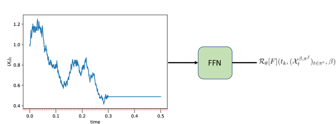
Figure 4.1. Diagram FFN network using stopped path as input

4.6.2. LSTM networks

Recurrent neural networks are a more natural approach to parametrise non-anticipative functionals, since their sequential output is adapted to the input, in the sense that $\mathcal{R}[F]_{\theta}(t_{k},(x_{t}^{\beta,\pi^{f}})_{t\in\pi^{c}})$ is built without looking into the future of the path at $t_{k}$ (Figure 4.2).

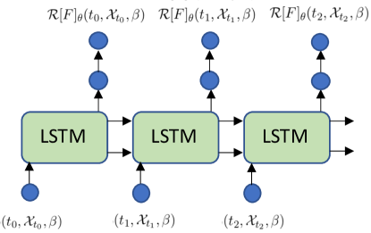
Figure 4.2. Diagram of LSTM network using path as input

Figure 4.3 displays the deep learning setting in the particular case where we use the stream of signatures (4.2) as an input to the LSTM network.

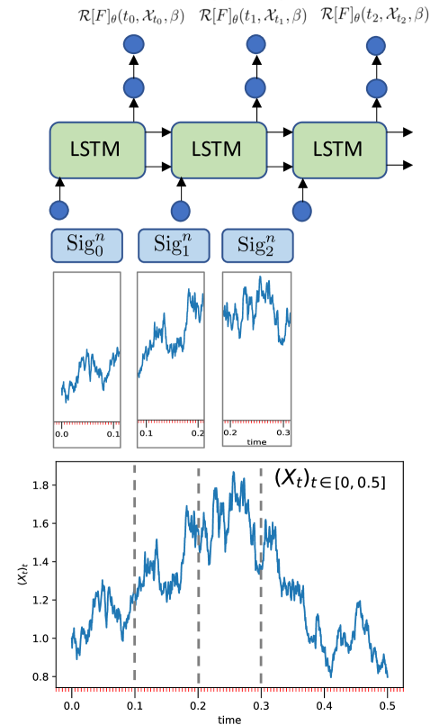
Figure 4.3. Diagram of LSTM network using path signature as input

4.7. Evaluation scheme

In this section we provide the evaluation measures of the deep solvers introduced in Algorithms 2 and 3.

4.7.1. Integral error of the option price parametrisation

We provide the absolute integral error of the solution of the path-dependent PDE, calculated on a test set for a fixed $\beta$. Recall that the Feynman–Kac formula tells us that the solution of the PPDE has a stochastic representation

$$F(t,\omega;\beta)=e^{-r(T-t)}\mathbb{E}\left[g((X_{t}^{\beta})_{t\in[0,T]};\beta)|(X_{t\wedge s}^{\beta})_{s\in[0,T]}=(\omega_{t\wedge s}^{\beta})_{s\in[0,T]}\right].$$

where $F:[0,T]\times C([0,T],\mathbb{R}^{d})\times B\to\mathbb{R}$ and the asset follows the the SDE (4.1). We denote by $F^{MC}:[0,T]\times\mathbb{R}^{N}\times B\to\mathbb{R}$ as the approximation of the price of the option calculated on a discretised path using $10^{6}$ Monte Carlo samples.

$$\mathcal{E}_{\text{integral}}^{\beta}=\mathbb{E}^{N_{\text{trn}}}\left[\sum_{t_{k}\in\pi^{c}}(t_{k+1}-t_{k})\cdot\left|F^{MC}\left(t_{k},(X_{t}^{\beta,\pi^{f}})_{t\in\pi^{c}};\beta\right)-\mathcal{R}[F]_{\theta}\left(t_{k},(\mathcal{X}_{t}^{\beta,\pi^{f}})_{t\in\pi^{c}};\beta\right)\right|\right].$$

4.7.2. Integral error of the hedging strategy parametrisation

We additionally evaluate the parametrisation of the hedging strategy in Algorithm 3 by calculating its absolute integral error

$$\mathcal{E}_{\text{hedging}}^{\beta}=\mathbb{E}^{N_{\text{trn}}}\left[\sum_{t_{k}\in\pi^{c}}(t_{k+1}-t_{k})\cdot\left|\nabla_{\omega}F^{MC}\left(t_{k},(X_{t}^{\beta,\pi^{f}})_{t\in\pi^{c}};\beta\right)-\mathcal{R}[\nabla_{\omega}F]_{\phi}\left(t_{k},(\mathcal{X}_{t}^{\beta,\pi^{f}})_{t\in\pi^{c}};\beta\right)\right|\right]$$

where we denote by $\nabla_{\omega}F^{MC}\left(t_{k},(X_{t}^{\beta,\pi^{f}})_{t\in\pi^{c}};\beta\right)$ as the approximation of the path derivative on a discretised path. It is approximated using $10^{6}$ Monte Carlo samples using (A.1).

4.7.3. Stochastic integral of the hedging strategy as a control variate

In Section 4.5, the discounted price is approximated by the estimator with low variance

$$M_{t}^{\text{cv},\phi}:=M_{T}-\int_{t}^{T}e^{-rs^{\prime}}\big{(}\mathcal{R}_{\phi}[\nabla_{\omega}F]\sigma\big{)}(s^{\prime},(s^{\prime},(X^{\beta}_{s^{\prime}\wedge s})_{s\in[0,T]};\beta)\,dW_{s^{\prime}}\,.$$

The correlation between the stochastic integral and $M_{T}$ should be close to $1$ in order to yield a good control variate (see  [23, Chapter 4.1]) and hence a good approximation of the hedging strategy. We provide the correlation between $M_{T}$ and the stochastic integral with $t=0$, and $x_{0}=1$.

$$\rho\left(M_{T},\int_{0}^{T}e^{-rs^{\prime}}\big{(}\mathcal{R}_{\phi}[\nabla_{\omega}F]\sigma\big{)}(s^{\prime},(s^{\prime},(X^{\beta}_{s^{\prime}\wedge s})_{s\in[0,T]};\beta)\,dW_{s^{\prime}}\right).$$

5. Numerical experiments

5.1. Black Scholes model and lookback option

Take a $d$-dimensional Wiener process $W$. We assume that we are given a symmetric, positive-definite matrix (covariance matrix) $\Sigma$ and a lower triangular matrix $C$ s.t. $\Sigma=CC^{*}$. The risky assets will have volatilities given by $\sigma^{i}$. We will (abusing notation) write $\sigma^{ij}:=\sigma^{i}C^{ij}$, when we don’t need to separate the volatility of a single asset from correlations. The risky assets under the risk-neutral measure are then given by

(5.1) $$dS^{i}_{t}=rS^{i}_{t}\,dt+\sigma^{i}S^{i}_{t}\sum_{j}C^{ij}dW^{j}_{t}\,.$$

Consider the lookback path-dependent payoff given by:

$$g\left((S_{t})_{t\in[0,T]}\right)=\left[\max_{t\in[0,T]}\sum_{i}S^{i}_{t}-\sum_{i}S^{i}_{T}\right]_{+}$$

We take $d=2$, $r=5\%$, $\Sigma^{ii}=1$, $\Sigma^{ij}=0$ for $i\neq j$. In our first two experiments where we learn the solution of the PPDE using Algorithms 2 and 3, we will try two different volatility values, $\sigma^{i}=30\%$ or $\sigma^{i}=100\%$. That is, in these two experiments we solve separetely two PPDEs, rather than a whole family of PPDEs. In the third experiment we solve a parametric family of PPDEs by sampling $\sigma^{i}$ from $[0,0.4]$.

We take the maturity time $T=0.5$. We divide the time interval $[0,T]$ in 1000 equal time steps in the fine time discretisation, i.e. $\pi^{f}=\{0=t_{0}<\ldots<t_{N}=T,N=1\,000\}$, and the following coarser time discretisation with 10 timesteps at which the network learns the prices: $\pi^{c}=\{0=t_{0}<\ldots<t_{10}=T\}\subset\pi^{f}$.

We train our models with batches of 200 random paths $(s_{t_{k}}^{i})_{n=0}^{N_{\text{steps}}}$ sampled from the SDE (5.1) using Euler scheme with $N_{\text{steps}}=100$. The assets’ initial values $s_{t_{0}}^{i}$ are sampled from a lognormal distribution $S_{0}\sim\exp((\mu-0.5\sigma^{2})\tau+\sigma\sqrt{\tau}\xi)$, where $\xi\sim\mathcal{N}(0,1),\mu=0.08,\tau=0.1$.

In our experiments, Feed-forward networks consist of four hidden layers with 100 neurons each each of them followed by the activation function ReLU$(x)=\max(0,x)$. If we use LSTM networks, then we append a feed-forward network to each output of the LSTM with two layers and ReLU activation functions, to ensure that each output of the model can take values in $\mathbb{R}^{m}$.

All the path signatures are calculated up to the fourth iterated integral, and are calculated on the path or on the lead-lag transform of the path (see Appendix B).

5.1.1. Experiment 1 - Learning conditional expectation (Algorithm 2)

We present results using the learning task (4.5), and different combinations of network architectures and network input. Results are shown in Table 1.

LSTM networks combined with path signatures consistently give better results than feedforward networks. It is remarkable from Figure 5.1 that one can see how path signatures start making a difference when the volatility of the underlying in the SDE (5.1) increases. Observe that the loss depicted in Figure 5.1 does not go down to 0. This comes from the fact that when we learn the conditional expectation, we are looking to find the $L^{2}$-distance between a random variable which is $\mathcal{F}_{T}$-measurable and its orthogonal projection on $\mathcal{F}_{t}\subsetneq\mathcal{F}_{T}$.

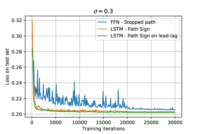
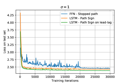
Figure 5.1. Loss on test set in terms of training iterations

Table 1. Evaluation of PPDE solver using algorithm 2.

Net. type	Net. input	$\sigma$	$\mathcal{E}_{\text{integral}}$
FFN (baseline)	Path	$0.3$	$8.64\times 10^{-3}$
LSTM	Path	$0.3$	$5.88\times 10^{-3}$
LSTM	Path sign	$0.3$	$5.75\times 10^{-3}$
LSTM	Path sign on lead-lag transf	$0.3$	$\mathbf{4.45\times 10^{-3}}$
FFN (baseline)	Path	1	$3.96\times 10^{-2}$
LSTM	Path	$1$	$3.09\times 10^{-2}$
LSTM	Path sign	$1$	$2.42\times 10^{-2}$
LSTM	Path sign on lead-lag transf	$1$	$\mathbf{1.73\times 10^{-2}}$

5.1.2. Experiment 2 - Learning Martingale Representation (Algorithm 3)

We present results using the learning task (4.9). Results are shown in Table 2. We observe in Table 1 that a combination of LSTM networks and path signatures provide the best results, and we restrict our experiments to this setting. We stress out that the obtained integral errors used in this method are slightly better than the errors we obtain after learning the conditional expectation (Table 1). We hypothesise that this is given due to higher structure of the solution contained in the loss function built to solve the BSDE.

Table 2. Evaluation of PPDE solver using algorithm 3.

Net. type	Net. input	$\sigma$	$\mathcal{E}_{\text{integral}}$	$\mathcal{E}_{\text{hedging}}$	$\rho$
LSTM	Path sign	$0.3$	$4.5\times 10^{-3}$	$2.02\times 10^{-4}$	$0.997$
LSTM	Path sign lead-lag	$\mathbf{0.3}$	$\mathbf{3.86\times 10^{-3}}$	$2.08\times 10^{-4}$	$\mathbf{0.998}$
LSTM	Path sign	$1$	$2.11\times 10^{-2}$	$3.3\times 10^{-3}$	$0.995$
LSTM	Path sign lead-lag	$\mathbf{1}$	$\mathbf{1.60\times 10^{-2}}$	$3.33\times 10^{-3}$	$0.994$

5.1.3. Experiment 3 - Learning parametric PPDE

: We incorporate the volatility $\sigma^{i},i=1,\ldots,d$ of the Black-Scholes model (5.1) as an input to the networks in order to solve a parametric family of PPDEs using Algorithm 3. $\sigma$ is uniformly sampled from $[0,0.4]$. Results in Table 3 show that parametric learning is shown to work as the error is consisten across the parameter range, with slightly higher errors for higher values of the volatility.

Table 3. Evaluation of parametric PPDE solver using using algorithm 3 and $\sigma$ as input to LSTM network

Method	$\sigma$	Net. type	Net. input	$\mathcal{E}_{\text{integral}}$	$\mathcal{E}_{\text{hedging}}$
Martingale repr.	0.05	LSTM	Path sign lead-lag	$6.47\times 10^{-3}$	$3.6\times 10^{-2}$
Martingale repr.	0.1	LSTM	Path sign lead-lag	$7.7\times 10^{-3}$	$1.4\times 10^{-2}$
Martingale repr.	0.15	LSTM	Path sign lead-lag	$8.16\times 10^{-3}$	$8.1\times 10^{-3}$
Martingale repr.	0.2	LSTM	Path sign lead-lag	$8.73\times 10^{-3}$	$6.4\times 10^{-3}$
Martingale repr.	0.25	LSTM	Path sign lead-lag	$9.3\times 10^{-3}$	$7.1\times 10^{-3}$
Martingale repr.	0.3	LSTM	Path sign lead-lag	$1.0\times 10^{-2}$	$7.5\times 10^{-3}$
Martingale repr.	0.35	LSTM	Path sign lead-lag	$1.07\times 10^{-2}$	$8.6\times 10^{-3}$

5.2. Heston model and autocallable option

In this experiment we consider the 1-dimensional Heston model with stochastic volatility

$$\begin{split}dS_{t}&=\sqrt{V_{t}}S_{t}dW_{t}^{S},\quad S_{0}=s_{0}\\ dV_{t}&=\kappa(\mu-V_{t})dt+\eta\sqrt{V_{t}}dW_{t}^{V},\quad V_{0}=v_{0},\\ d\langle W^{S},W^{V}\rangle_{t}&=\rho dt\end{split}$$

where we take $\kappa=3$, $\mu=0.3$, $\eta=1$, $\rho=0.6$, $v_{0}=s_{0}=1$.

We aim to price an autocallable option (see for example [1]) on $(S_{t})_{t\in[0,T]}$. Consider $m$ observation dates, $t_{1}<\ldots<t_{m}$, a barrier value $B$, premature payoffs $Q_{1},\ldots,Q_{m}$, and a redempetion payoff $q(s)$.

Given a path $(S_{t})_{t\in[0,T]}$ and the corresponding prices at the observation dates $S_{t_{1}},\ldots,S_{t_{m}}$ then the discounted payoff of the univariate autocallable option is given by:

$$g((S_{t})_{t\in[0,T]})=\begin{cases}Q_{j}\quad\text{if}\quad S_{t_{i}}<B\leq S_{t_{j}}\quad\forall i<j,\\ q(S_{m})\quad\text{if}\quad S_{t_{j}}<B\quad\forall j\end{cases}$$

The price of the autocallable option at current time $\tau$ is given by its expected (discounted) payoff. For example, if the option has 2 observation times, and $\tau=0$, then

$$\begin{split}F(t,(s_{t\wedge\tau})_{\tau\in[0,T]})&:=\mathbb{E}[g\left((S_{t})_{t\in[0,T]}\right)|(S_{t\wedge\tau})_{\tau\in[0,T]}=(s_{t\wedge\tau})_{\tau\in[0,T]}]\\ &=Q_{1}\mathbb{E}[\mathds{1}_{B\leq S_{t_{1}}/S_{0}}]+Q_{2}\mathbb{E}[\mathds{1}_{B>S_{t_{1}}/S_{0}}\mathds{1}_{B\leq S_{t_{2}}/S_{0}}]+\mathbb{E}[q(S_{T})\mathds{1}_{B>S_{t_{1}}/S_{0}}\mathds{1}_{B>S_{t_{2}}/S_{0}}]\\ \end{split}$$

We use the parameters in table 4 for the option payoff.

Table 4. Parameters of the autocallable option

Parameter	Value
Maturity	$T=0.5$ years
Barrier	$B=1.02$
No. of observation dates	$m=2$
Observation dates	2,4 months
Premature payoffs	$Q_{1}=1.1,Q_{2}=1.2$
Redemption payoff	$q(s)=0.9s$

Results of the approximation of the PPDE using Algorithm 3 are provided in Table 5. Figure 5.2 displays the Monte Carlo approximation of the PPDE solution and the LSTM approximation

Table 5. Evaluation of PPDE solver using Heston model, autocallable option and algorithm 3.

Method	Net. type	Net. input	$\mathcal{E}_{\text{integral}}$	$\mathcal{E}_{\text{hedging}}$	$\rho$
Martingale repr.	LSTM	Path sign lead-lag	$1.4\times 10^{-2}$	$1.8\times 10^{-2}$	$0.948$

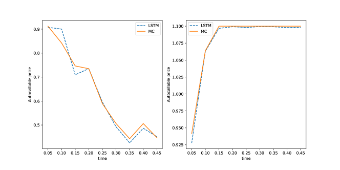
Figure 5.2. Monte Carlo price and predicted price using LSTM networks trained using the Martingale representation of the price for two different paths of the underlying share

6. Conclusions

In this paper we implement two numerical methods to approximate the solution of a parametric family of PPDEs.

$$\begin{split}&\bigg{[}\partial_{t}F+b\nabla_{\omega}F+\frac{1}{2}\text{tr}\left[\nabla_{\omega}^{2}F\sigma^{*}\sigma\right]-rF\bigg{]}(t,\omega;\beta)=0\,,\\ &F(T,\omega;\beta)=g(\omega;\beta)\,,\,\,\,t\in[0,T]\,,\,\,\omega\in C([0,T];\mathbb{R}^{d})\,,\,\,\beta\in B\,.\end{split}$$

by using the probabilistic representation of $F(t,\omega;\beta)$ given by Feynman-Kac formula. This representation allows to tackle the problem of solving the PPDE, as pricing an option where the underlying asset follows a certain SDE in the risk neutral measure. This is the setting of our numerical experiments, where we price lookback and autocallable options using properties of the conditional expectation (algorithm 2) or the martingale representation of the price (algorithm 3). In the latter algorithm, we parametrise $\nabla_{\omega}F$ by a neural network, which in some models provides the hedging strategy. We combine path signatures to encode the information in $\omega$ in some finite dimensional structure together with LSTM networks to model non-anticipative functionals, that in our experiments provide a higher accuracy than Feed Forward Networks.

Appendix A Functional Ito Calculus

In this section we define the notion of path-dependent PDE. and we review the theory that it relies on, Functional Ito calculus [18, 2]. Consider the space of càdlàg paths in $[0,T]$, $D([0,T],\mathbb{R}^{d})$. The space of stopped paths is the quotient space

$$\Lambda_{T}:=\left([0,T]\times D([0,T],\mathbb{R}^{d})\right)/\sim$$

defined by the equivalence relationship

$$(t,\omega)\sim(t^{\prime},\omega^{\prime})\Leftrightarrow t=t^{\prime}\text{ and }(\omega_{s\wedge t})_{s\in[0,T]}=(\omega^{\prime}_{s\wedge t})_{s\in[0,T]}.$$

Consider a functional $F:\Lambda_{T}\rightarrow\mathbb{R}$. The continuity of $F$ is defined with respect to the metric in $\Lambda_{T}$:

$$d_{\infty}((t,\omega),(t^{\prime},\omega^{\prime}))=\sup_{s\in[0,T]}|\omega_{s\wedge t}-\omega^{\prime}_{s\wedge t^{\prime}}|+|t-t^{\prime}|$$

Furthermore, a functional $F$ is boundedness preserving if for every compact set $K\subset\mathbb{R}^{n}$, and $\forall t_{0}\in[0,T]$ there exists a constant $C>0$ depending on $K,t_{0}$ such that

$$\forall t\in[0,t_{0}],\quad\forall(t,\omega)\in\Lambda_{T},\quad(\omega_{s})_{s\in[0,t]}\subset K\Rightarrow F(t,\omega)<C.$$

And finally we define, when the limit, exists the horizontal derivative of a functional $F$

$$\partial_{t}F(t,\omega):=\lim_{h\rightarrow 0^{+}}\frac{F(t+h,\omega)-F(t,\omega)}{h}$$

and the vertical derivative

(A.1) $$\nabla_{\omega}F(t,\omega):=(\partial_{i}F(t,\omega),i=1,\ldots,d)\in\mathbb{R}^{d}$$

where

$$\partial_{i}F(t,\omega):=\lim_{h\rightarrow 0}\frac{F(t,(\omega_{t\wedge s})_{s\in[0,T]}+he_{i}\mathbf{1}_{[t,T]})-F(t,(\omega_{t\wedge s})_{s\in[0,T]})}{h}$$

with $e_{i}$ the canonical basis of $\mathbb{R}^{d}$. The functional $\nabla_{\omega}F:\Lambda_{T}\rightarrow\mathbb{R}^{d}$ is well defined in the quotioent space $\Lambda_{T}$, and therefore one can calculate higher order path derivatives by repeating the same operation when the limit exists.

A functional $F:\Lambda_{T}\rightarrow\mathbb{R}$ belongs to $\mathbb{C}^{1,2}$ if:

1. It is continuous.

2. It is boundedness preserving.

3. It has continuous, boundedness preserving derivatives $\partial_{t}F,\nabla_{\omega}F,\nabla_{\omega}^{2}F$.

Appendix B The signature of a path

Iterated integrals of piece-wise regular multi-dimensional paths were first studied by K.T. Chen [10, 11], and the study of their properties was extended for continuous paths of bounded variation in [27].

Given a $d$-dimensional path $X:[a,b]\rightarrow\mathbb{R}^{d}$, we denote the coordinate paths $(X_{t}^{1},\ldots,X_{t}^{d})$ where each $X^{i}:[a,b]\rightarrow\mathbb{R}$.

For each $i=1,\ldots,d$ the first iterated integral of the $i$-th coordinate path is

$$S(X)^{i}_{a,t}:=\int_{a<s<t}dX^{i}_{s}=X^{i}_{t}-X^{i}_{a}.$$

Note that since $S(X)^{i}_{[a,\cdot]}:[a,b]\rightarrow\mathbb{R}$ is also a continuous path, we can integrate it again along any of the coordinate paths to obtain the second iterated integral: for any $i,j$,

$$S(X)^{i,j}_{a,t}:=\int_{a<s<t}S(X)^{i}_{a,s}dX^{j}_{s}=\int_{a<r<s<t}dX^{i}_{r}dX^{j}_{s}.$$

This process can be repeated to obtain any coordinate of the $k$-th iterated integral:

$$S(X)^{i_{1},\ldots,i_{k}}_{a,t}=\int_{a<t_{1}<t_{2}<\ldots<t_{k}<t}dX_{t_{1}}^{i_{1}}\ldots dX_{t_{k}}^{i_{k}}$$

We introduce the concept of tensor algebera $T((\mathbb{R}^{d}))$, which is where the signature of an $\mathbb{R}^{d}$-valued path takes its values.

Definition B.1.

Consider the basis of a vector space $E$ given by $\{e_{1},e_{2},\ldots,e_{d}\}$, and the successive tensor powers $E^{\otimes n}$, which can be identified with the space of degree $n$ in $d$ variables

$$\sum_{i_{1}\ldots i_{n}\in\{1,\ldots,d\}}\lambda_{i_{1},\ldots,i_{n}}e_{i_{1}}\ldots e_{i_{n}}$$

The tensor algebra space denoted by $T((E))$ is then defined as

$$T((E)):=\left\{(a_{0},a_{1},\ldots,a_{n},\ldots)\,|\,\forall n\geq 0,a_{n}\in E^{\otimes n}\right\}$$

The $n$-th truncated tensor algebra space is

$$T^{n}(E):=\bigoplus_{i=1}^{n}E^{\otimes n}$$

Thus, the $k$-th iterated integral of $X$ can be defined as

$$S(X)_{a,t}^{(k)}=\int_{a<t_{1}<t_{2}<\ldots<t_{k}<t}dX_{t_{1}}\otimes\ldots\otimes dX_{t_{l}}\in T^{k}(\mathbb{R}^{d})$$

Definition B.2.

Let $\mathcal{I}$ denote all the set of multi-indices $(i_{1},\ldots,i_{k})$ with $k\geq 0$ and $i_{j}\in\{1,\ldots,d\}$. The signature of $X:[a,b]\rightarrow\mathbb{R}^{d}$ is an element of the tensor algebra $T((\mathbb{R}^{d}))$,

$$\text{Sig}_{a,b}(X)=(S(X)^{I}_{a,b})_{I\in\mathcal{I}}=(1,S(X)_{a,t}^{(1)},S(X)_{a,t}^{(2)},\ldots)\in T((\mathbb{R}^{d})).$$

B.1. The signature of a data stream

So far we have built the path signature on continuous trajectories. In financial data, one normally deals with data streams, i.e. trajectories defined by a sequence of time points $(x^{\pi}_{t_{i}})_{i=1,\ldots,N}$. The common approach to define the signature of this data stream is via the iterated integrals of its piece-wise linear interpolation.

B.2. Machine Learning and the signature method

For a premier on the use of the signature in Machine Learning, we refer the reader to [12] and for a rigorous treatment of the signature properties the reader can refer to [27]. We state however the following two properties that motivate using the signature of a path in Machine Learning.

1. The terms of the signature decay in size factorially [37, Lemma 2.1.1], i.e.

   $$\left\|S(X)_{a,t}^{(k)}\right\|\leq\frac{C(X)^{k}}{k!}$$

   where $C(X)$ depends on $X:[a,b]\rightarrow\mathbb{R}^{d}$ and $\|\cdot\|$ is a tensor norm in $T^{k}(\mathbb{R}^{d})$. As a consequence of this, it is usual in machine learning to truncate the signature up until a certain depth $n$, obtaining

   $$\text{Sig}^{(n)}_{[a,b]}(X)=(1,S(X)_{a,t}^{(1)},S(X)_{a,t}^{(2)},\ldots,S(X)_{a,t}^{(n)})$$

2. The signature is rich enough that every continuous function of the path can be approximated by a linear function of its truncated signature. More precisely, the universality result given in Theorem 3.1 of  [35] tells us that any continuous functional on the paths can be approximated up until any accuracy $\varepsilon$ by a linear combination of the coordinates of the truncated path signature $\text{Sig}^{(n)}_{[a,b]}(X)$, for some $n:=n_{\varepsilon}$.

B.3. Lead-lag transform

We finally introduce the lead-lag transform of a a data stream  [21], that to write Ito integrals as linear functionals on the signature of the lead-lag transformed path.

More specifically, given a stream of data $(x^{\pi}_{t_{i}})_{i=1,\ldots,N}$, then we define the lead-transformed stream as

$$x^{\pi,\text{lead}}_{j}=\begin{cases}x^{\pi}_{t_{i}}\text{ if }j=2i\\ x^{\pi}_{t_{i}}\text{ if }j=2i-1\end{cases}$$

and the lag-transformed stream as

$$x^{\pi,\text{lag}}_{j}=\begin{cases}x^{\pi}_{t_{i}}\text{ if }j=2i\\ x^{\pi}_{t_{i}}\text{ if }j=2i+1\end{cases}.$$

The resulting lead-lag transformed stream is:

$$(x^{\pi,\text{lead-lag}}_{t_{i}})_{i=1,\ldots,2N}=(x^{\pi,\text{lead}}_{t_{i}},x^{\pi,\text{lag}}_{t_{i}})_{i=1,\ldots,2N}.$$

Appendix C Deep Neural Networks for function approximation

C.1. Feedforward neural networks

A fully connected artificial neural network is given by by a composition of affine transformations and non-linear activation functions. Fix $L$ as the number of layers, then the space of parameters of the network is given by

$$\Pi=(\mathbb{R}^{l^{1}\times l^{0}}\times\mathbb{R}^{l^{1}})\times(\mathbb{R}^{l^{2}\times l^{1}}\times\mathbb{R}^{l^{2}})\times\cdots\times(\mathbb{R}^{l^{L}\times l^{L-1}}\times\mathbb{R}^{l^{L}})\,,$$

hence if we denote the parameters of a network by

$$\theta:=((W^{1},b^{1}),\ldots,(W^{L},b^{L}))\in\Pi\,.$$

and by denoting the $i$-th network layer by $M^{i}$ such that

$$M^{i}(z_{i-1})=\varphi^{i}(W^{i}z_{i-1}+b^{i})$$

with $\varphi$ being a non-linear activation function such as $\tanh$ or the sigmoid, then the reconstruction of $\mathcal{R}_{\theta}:\mathbb{R}^{l^{0}}\to\mathbb{R}^{l^{L}}$ can be written recursively by

(C.1) $$y:=\mathcal{R}_{\theta}(z_{0})=W^{L}z^{L-1}+b^{L}\,,\,\,\,\,z^{k}=M^{k}(z_{k-1})\,.$$

C.2. Long Short Term Memory Networks

Long Short Term Memory (LSTM) networks [30] are an example of Recurrent Neural Networks, which are useful when the input is a sequence of points

$$\{x_{0},x_{1},\ldots,x_{n}\}.$$

Each element $x_{t}$ of the input sequence is fed to the Recurrent Neural Network which in addition to returning an output $y_{t}$, also stores some information (or hidden state) $a_{t}$ that is used to perform computations in the next step: More formally,

$$\mathcal{R}_{\theta}(x_{t},a_{t-1})=(y_{t},a_{t}).$$

LSTM networks are designed to tackle the problem of exploding or vanishing gradients that plain RNN suffer from (see[7]). They do this by regulating the information carried forward by the hidden state given each input of the sequence, using the so-called gates. Specifically, the operations performed for the $i$-th element of the sequence $x_{i}$, receiving the hidden state $a_{t-1}:=(h_{t-1},c_{t-1})$ are:

$$i_{t} =\sigma(W_{xi}x_{t}+b_{xi}+W_{hi}h_{t-1}+b_{hi})$$

$$f_{t} =\sigma(W_{xf}x_{t}+b_{xf}+W_{hf}h_{t-1}+b_{hf})$$

$$g_{t} =\tanh(W_{xg}x_{t}+b_{xg}+W_{hg}h_{t-1}+b_{hg})$$

$$o_{t} =\sigma(W_{xo}x_{t}+b_{xo}+W_{ho}h_{t-1}+b_{ho})$$

$$c_{t} =f_{t}\odot c_{t-1}+i_{t}\odot g_{t}$$

$$h_{t} =o_{t}\odot\tanh(c_{t})$$

in addition, since $h_{t}\in(0,1)$, we add a linear layer

$$y_{t}=W_{hy}h_{t}+b_{hy}.$$

Where $x_{t}\in\mathbb{R}^{d},W_{x*}\in\mathbb{R}^{k\times d},b_{x*}\in\mathbb{R}^{k}$, $k\in\mathbb{Z}_{+}$, and $\odot$ is the element-wise multiplication of two vectors.

References

• [1] T. Alm, B. Harrach, D. Harrach, and M. Keller. A Monte Carlo pricing algorithm for autocallables that allows for stable differentiation. Journal of Computational Finance, 17(1), 2013.
• [2] V. Bally, L. Caramellino, R. Cont, F. Utzet, and J. Vives. Stochastic integration by parts and functional Itô calculus. Springer, 2016.
• [3] C. Bayer and B. Stemper. Deep calibration of rough stochastic volatility models, 2018.
• [4] C. Beck, S. Becker, P. Cheridito, A. Jentzen, and A. Neufeld. Deep splitting method for parabolic PDEs, 2019.
• [5] C. Beck, W. E, and A. Jentzen. Machine Learning Approximation Algorithms for High-Dimensional Fully Nonlinear Partial Differential Equations and Second-order Backward Stochastic Differential Equations. Journal of Nonlinear Science, 29(4):1563–1619, Jan 2019.
• [6] C. Beck, L. Gonon, and A. Jentzen. Overcoming the curse of dimensionality in the numerical approximation of high-dimensional semilinear elliptic partial differential equations, 2020.
• [7] Y. Bengio, P. Simard, and P. Frasconi. Learning long-term dependencies with gradient descent is difficult. IEEE transactions on neural networks, 5(2):157–166, 1994.
• [8] J. Berner, P. Grohs, and A. Jentzen. Analysis of the Generalization Error: Empirical Risk Minimization over Deep Artificial Neural Networks Overcomes the Curse of Dimensionality in the Numerical Approximation of Black–Scholes Partial Differential Equations. SIAM Journal on Mathematics of Data Science, 2(3):631–657, Jan 2020.
• [9] Q. Chan-Wai-Nam, J. Mikael, and X. Warin. Machine Learning for semi linear PDEs, 2018.
• [10] K.-T. Chen. Integration of paths, geometric invariants and a generalized Baker-Hausdorff formula. Annals of Mathematics, pages 163–178, 1957.
• [11] K.-T. Chen. Integration of paths–a faithful representation of paths by noncommutative formal power series. Transactions of the American Mathematical Society, 89(2):395–407, 1958.
• [12] I. Chevyrev and A. Kormilitzin. A primer on the signature method in machine learning. arXiv preprint arXiv:1603.03788, 2016.
• [13] S. N. Cohen and R. J. Elliott. Stochastic calculus and applications. Springer, 2015.
• [14] R. Cont and D. Fournie. A functional extension of the Ito formula. Comptes Rendus Mathematique, 348(1-2):57–61, 2010.
• [15] R. Cont and D.-A. Fournié. Functional Itô calculus and stochastic integral representation of martingales. The Annals of Probability, 41(1):109–133, Jan 2013.
• [16] R. Cont and Y. Lu. Weak approximation of martingale representations. Stochastic Processes and their Applications, 126(3):857–882, 2016.
• [17] C. Cuchiero, W. Khosrawi, and J. Teichmann. A Generative Adversarial Network Approach to Calibration of Local Stochastic Volatility Models. Risks, 8(4):101, Sep 2020.
• [18] B. Dupire. Functional Itô calculus. Quantitative Finance, 19(5):721–729, 2019.
• [19] W. E, J. Han, and A. Jentzen. Deep Learning-Based Numerical Methods for High-Dimensional Parabolic Partial Differential Equations and Backward Stochastic Differential Equations. Communications in Mathematics and Statistics, 5(4):349–380, Nov 2017.
• [20] W. E, J. Han, and A. Jentzen. Algorithms for Solving High Dimensional PDEs: From Nonlinear Monte Carlo to Machine Learning, 2020.
• [21] G. Flint, B. Hambly, and T. Lyons. Discretely sampled signals and the rough Hoff process. Stochastic Processes and their Applications, 126(9):2593–2614, Sep 2016.
• [22] P. Gierjatowicz, M. Sabate-Vidales, D. Šiška, L. Szpruch, and Žan Žurič. Robust pricing and hedging via neural SDEs, 2020.
• [23] P. Glasserman. Monte Carlo methods in financial engineering. Springer, 2013.
• [24] L. Gonon, P. Grohs, A. Jentzen, D. Kofler, and D. Šiška. Uniform error estimates for artificial neural network approximations for heat equations, 2020.
• [25] I. Goodfellow, Y. Bengio, A. Courville, and Y. Bengio. Deep Learning. MIT press, 2016.
• [26] P. Grohs, F. Hornung, A. Jentzen, and P. von Wurstemberger. A proof that artificial neural networks overcome the curse of dimensionality in the numerical approximation of black-scholes partial differential equations, 2018.
• [27] B. Hambly and T. Lyons. Uniqueness for the signature of a path of bounded variation and the reduced path group. Annals of Mathematics, pages 109–167, 2010.
• [28] J. Han, A. Jentzen, et al. Solving high-dimensional partial differential equations using deep learning. arXiv:1707.02568, 2017.
• [29] A. Hernandez. Model calibration with neural networks. Available at SSRN 2812140, 2016.
• [30] S. Hochreiter and J. Schmidhuber. Long short-term memory. Neural computation, 9(8):1735–1780, 1997.
• [31] B. Horvath, A. Muguruza, and M. Tomas. Deep Learning Volatility, 2019.
• [32] C. Huré, H. Pham, and X. Warin. Deep backward schemes for high-dimensional nonlinear PDEs, 2020.
• [33] A. Itkin. Deep learning calibration of option pricing models: some pitfalls and solutions, 2019.
• [34] A. Jacquier and M. Oumgari. Deep PPDEs for rough local stochastic volatility, 2019.
• [35] D. Levin, T. Lyons, and H. Ni. Learning from the past, predicting the statistics for the future, learning an evolving system, 2013.
• [36] S. Liu, A. Borovykh, L. A. Grzelak, and C. W. Oosterlee. A neural network-based framework for financial model calibration. Journal of Mathematics in Industry, 9(1), Sep 2019.
• [37] T. J. Lyons, M. Caruana, and T. Lévy. Differential equations driven by rough paths. Springer, 2007.
• [38] W. A. McGhee. An artificial neural network representation of the SABR stochastic volatility model. Available at SSRN 3288882, 2018.
• [39] H. Pham, X. Warin, and M. Germain. Neural networks-based backward scheme for fully nonlinear PDEs, 2019.
• [40] M. Raissi, P. Perdikaris, and G. E. Karniadakis. Physics-informed neural networks: A deep learning framework for solving forward and inverse problems involving nonlinear partial differential equations. Journal of Computational Physics, 378:686–707, 2019.
• [41] Y. F. Saporito and Z. Zhang. PDGM: a Neural Network Approach to Solve Path-Dependent Partial Differential Equations, 2020.
• [42] J. Sirignano and K. Spiliopoulos. DGM: A deep learning algorithm for solving Partial Differential Equations. arXiv:1708.07469, 2017.
• [43] H. Stone. Calibrating rough volatility models: a convolutional neural network approach, 2019.
• [44] M. S. Vidales, D. Siska, and L. Szpruch. Unbiased deep solvers for parametric PDEs, 2018.