Inferring the concentration of dark matter subhalos perturbing strongly lensed images

Abstract

We demonstrate that the perturbations of strongly lensed images by low-mass dark matter subhalos are significantly impacted by the concentration of the perturbing subhalo. For subhalo concentrations expected in $\Lambda$CDM, significant constraints on the concentration can be obtained at HST resolution for subhalos with masses larger than about $10^{10}M_{\odot}$. Constraints are also possible for lower mass subhalos, if their concentrations are higher than the expected scatter in CDM. We also find that the concentration of lower mass perturbers down to $\sim 10^{8}M_{\odot}$ can be well-constrained with a resolution of $\sim 0.01^{\prime\prime}$, which is achievable with long-baseline interferometry. Subhalo concentration also plays a critical role in the detectability of a perturbation, such that only high concentration perturbers with mass $\lesssim 10^{9}M_{\odot}$ are likely to be detected at HST resolution. If scatter in the $\Lambda$CDM mass-concentration relation is not accounted for during lens modeling, the inferred subhalo mass can be biased by up to a factor of 3(6) for subhalos of mass $10^{9}M_{\odot}$($10^{10}M_{\odot}$); this bias can be eliminated if one varies both mass and concentration during lens fitting. Alternatively, one may robustly infer the projected mass within the subhalo’s perturbation radius, defined by its distance to the critical curve of the lens being perturbed. With a sufficient number of detections, these strategies will make it possible to constrain the halo mass-concentration relation at low masses in addition to the mass function, offering a probe of dark matter physics as well as the small-scale primordial power spectrum.

1. Introduction

A key prediction of the Cold Dark Matter (CDM) paradigm is the existence of a large number of dark matter subhalos around galaxies, with masses that go down to $<1M_{\odot}$ for the smallest halos (Green et al., 2004). The vast majority of these subhalos are expected to be entirely devoid of stars, as their primordial gas would have been heated sufficiently by the ultraviolet background during reionization to escape the shallow potential wells of these subhalos. In the past few years, hydrodynamical cosmological simulations that include radiative transfer effects have estimated that star formation is suppressed entirely in dark matter halos with virial masses lower than $10^{8}$-$10^{9}M_{\odot}$ (Sawala et al., 2016), where the exact threshold depends on the details of the gas heating and cooling. The observed ultrafaint satellites of the Milky Way galaxy, such as those recently discovered in the Dark Energy Survey (Bechtol et al., 2015), are thus expected to inhabit dark matter halos that lie just above this threshold (Brown et al., 2014). Detecting a large population of dark matter halos with masses $\lesssim 10^{9}M_{\odot}$ is thus a crucial test of CDM.

Many well-motivated particle models for dark matter diverge from the CDM paradigm, with very different predictions for small-scale structure. For example, in warm dark matter models (WDM), the thermal motion of free-streaming dark matter particles erased small-scale structure before nonlinear collapse would have occurred; as a result, the number of dark matter subhalos is suppressed below a particular mass threshold (typically below $\sim 10^{9}M_{\odot}$ for viable models; Bose et al. 2017), and galaxies form with lower central densities (Lovell et al., 2014). In hidden sector models, dark matter particles can interact among themselves via a hidden force (Feng et al., 2009). A sufficiently high self-interaction cross section can lower the central density of low-mass halos and subhalos compared to that of CDM (Rocha et al., 2013; Elbert et al., 2014). However, the particle model of dark matter is not the only possible factor that can alter the small-scale matter power spectrum: certain types of inflation models can produce a running (departure from power law) in the primordial power spectrum (Kobayashi & Takahashi, 2011; Ashoorioon & Krause, 2006; Minor & Kaplinghat, 2015), suppressing power at small scales Garrison-Kimmel et al. 2014). Whether primordial or through late-time effects, all of these alternative cosmological paradigms make distinct predictions for both the abundance and central densities of dark matter halos of a given mass.

Strong gravitational lensing provides a powerful probe of the dark matter distribution on dwarf galaxy scales, since the lensed images of a background source can undergo visible perturbations due to the presence of dark matter subhalos as well as dark matter halos that lie along the line of sight to the lens galaxy. Recently a few detections of dark substructures in gravitational lenses have been reported by observing their effect on highly magnified images. Two of these were discovered in the SLACS dataset (Vegetti et al., 2010, 2012), while more recently, a subhalo was reported by Hezaveh et al. (2016) to have been detected in an ALMA image of the lens system SDP.81 (ALMA Partnership et al., 2015). In order to test the expected mass function of halos in CDM, a robust estimate of the mass of these perturbing dark matter halos is very important; unfortunately however, the total inferred mass of the perturbers is highly dependent on their assumed density profile and tidal radius (Minor et al., 2017; Vegetti et al., 2014). One approach to test CDM is to simply assume that the perturbers follow a Navarro-Frenk-White (NFW) profile (or a truncated form thereof), since the dark matter halos in CDM N-body simulations are well fit by this profile (Navarro et al., 1996). This approach is supported by recent results from hydrodynamical simulations that subhalos below $10^{9}M_{\odot}$ are near the threshold for star formation and hence may not be significantly altered by baryon physics (Fitts et al., 2017; Sawala et al., 2016; Ocvirk et al., 2016). Even under this assumption, however, there is some expected scatter in the central density of halos of a given mass, embodied by the concentration parameter $c_{200}=r_{200}/r_{s}$; hence, assuming that subhalos follow a tight mass-concentration relation without scatter may also bias the inferred masses.

Estimating the mass of a perturbing subhalo is not the only quantity of importance, however. We argue that constraining the concentration of perturbing dark matter subhalos is equally important as the total mass, since different particle models for dark matter (or even inflation physics) can differ widely in their predictions for the central densities of dark matter halos (Lovell et al., 2014; Rocha et al., 2013). Thus, an important question is whether the concentration of perturbing dark matter halos can be meaningfully constrained in addition to their masses. If the perturber’s concentration significantly affects the strength of the perturbation to the local lensing deflection, then in principle meaningful constraints on the concentration are possible. Indeed, recently Gilman et al. (2020) have shown that constraints on subhalo concentrations are possible for lensed quasars, at least in a statistical sense. If concentrations of individual subhalos can be constrained from their perturbations of lensed arcs, this approach may not only achieve a more robust mass estimate, but may provide an additional probe of the small-scale power spectrum beyond simply testing the CDM halo mass function.

In this paper we simulate and model hundreds of mock lensing data to investigate the effect of dark matter subhalo concentration on lensing perturbations. We show that constraints on dark matter subhalo concentrations are indeed possible, and provide a powerful probe of the small-scale matter power spectrum. In addition, we will show that making the approximation that subhalos follow an exact mass-concentration relation (without scatter) during modeling of substructure perturbations can result in biased mass inferences, by up to a factor of $\sim$6 or so. Hence, even if dark matter is indeed cold and collisionless, scatter in the mass-concentration relation cannot be ignored if one aims to test the expected CDM halo mass function at dwarf galaxy scales via strong lensing.

We organize the paper as follows: in Section 2, we describe our lens modeling software and simulated data. In Section 3 we investigate how well the perturber’s concentration can be constrained, both at HST resolutions as well as at higher resolutions expected from next-generation telescopes. In Section 4, we will investigate the effect of halo concentration on the detectability of substructure perturbations. In Section 5 we will discuss the physical interpretation of the degeneracy between mass and concentration in terms of the size of the subhalo’s lensing perturbation. Next, in Section 6.1 we explore the expected bias (in CDM) in the inferred perturber’s mass if scatter in halo concentration is unaccounted for, while in Section 6.2 we demonstrate that bias in these cases is eliminated by using the mass estimator of Minor et al. (2017). Finally, in Section 7 we discuss the physical interpretation of the concentration constraints, and in Section 8 we discuss the effect of tidal stripping on our results. We conclude in Section 9.

2. Lens modeling and mock data

2.1. Lens simulation and modeling procedure

To investigate the effect of subhalo concentration, we generate a grid of mock data that explores a variety of different subhalo masses, concentrations, positions in the lens plane, and lens redshifts. For the primary lens we use a power-law ellipsoidal projected density profile, plus an external shear term in the potential. We adopt parameters such that it closely resembles the lens SDSSJ0946+1006, for which Vegetti et al. (2010) detected a perturbing subhalo. For our primary mock data grid, we generate simulated images using the pixel size of the Hubble Space Telescope (HST) ACS camera ($0.045^{\prime\prime}$) and the actual HST point-spread function (PSF) pixel map used by Vegetti et al. (2010). For a small subset of these data, we will also generate and model a high-resolution version with $0.01^{\prime\prime}$ pixel size (described in Section 3.2). The source galaxy is created using an elliptical Gaussian profile with two possible sizes, corresponding to unlensed widths of 0.03 and 0.06 arcseconds.

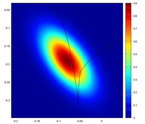
(a) mock source

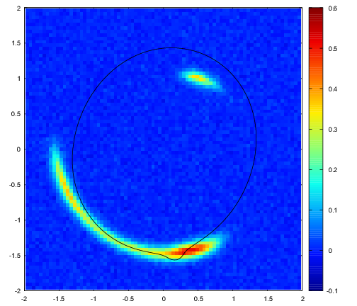
(b) mock data image

Figure 1.— Mock source and data image, with a $10^{10}M_{\odot}$ perturber. In panel (a) the mock source is shown with caustic overlaid; note the kink in the caustic generated by the perturbing subhalo. In panel (b) the mock image is shown with critical curve overlaid, where a perturbation is evident in the lower arc.

In our primary mock data images, the subhalo is modeled using a spherical Navarro-Frenk-White (NFW) profile (Navarro et al., 1996), without any tidal truncation. As we show in Section 8, for the majority of subhalo perturbations we expect the subhalo’s tidal radius to be much larger than its NFW scale radius, since the most subhalos will be several tens to hundreds of kiloparsecs away from the host galaxy center (Minor et al., 2017). Since the Einstein radius of the lens typically corresponds to a few kiloparsecs in the lens plane, most of that distance lies along the line of sight to the lens plane, i.e. the plane containing the center of the host galaxy. Thus, in most cases the tidal radius will not affect the lensing dramatically, however we will investigate the effect of tidal truncation in detail in Section 8.

Since the Hubble PSF is relatively undersampled compared to the pixel size, the images produced can be sensitive to how the ray-tracing is done, particularly near the critical curve. To mitigate this, we split each image pixel into N$\times$N subpixels and ray-trace the center point of each subpixel to the source plane, assigning it the surface brightness given by the source profile at the position of the ray-traced point. These surface brightness values are then averaged to find the surface brightness of the image pixel. After the ray-tracing is complete, the resulting pixel values are then convolved with the PSF and Gaussian noise is added (similar to the noise level in SDSSJ0946+1006) to generate the mock image. An example with a $10^{10}M_{\odot}$ perturber is shown in Figure 1. We find that 3$\times$3 splitting achieves sufficient accuracy without adding too much computational burden; a greater number of subpixels changes the surface brightness values very little while adding significant computational cost.

Our primary method for modeling the mock data uses a parameterized surface brightness profile, with the ray tracing as outlined above. This allows for relatively rapid exploration of the parameter space, which consists of both lens and source model parameters, hence reducing computational cost compared to reconstructing pixellated sources. However, for the purposes of constraining the detailed properties of subhalos, using an elliptical Gaussian profile would be too restrictive a prior, for two reasons: 1) actual galaxies rarely (if ever) have perfectly elliptical contours and Gaussian profiles; 2) even if the true source is Gaussian (as with our mock data), if one is modeling a subhalo with an incorrect mass or concentration, this systematic can often be (at least partially) absorbed into the inferred source galaxy by perturbing the isophotes or deviating from a Gaussian profile. This is also the case if the data are perturbed by a subhalo and one is not including a subhalo in the model at all. Thus, if one does not allow enough freedom in the source galaxy model, the constraints on concentration and mass may appear stronger than they really are.

For our modeling runs where we focus on constraining the concentrations of subhalos (Sections 3.1 and 3.2), we therefore adopt the following approach: we start with a Sersic profile where the isophotes are “generalized ellipses” with a radial coordinate defined by

$$r_{0}(x,y)=\left(|x-x_{0}|^{C_{0}+2}+\left|\frac{y-y_{0}}{q}\right|^{C_{0}+2}\right)^{\frac{1}{C_{0}+2}}$$ (1)

where $q$ is the axis ratio and $C_{0}$ is the “boxiness” parameter, such that $C_{0}=0$ corresponds to a perfectly elliptical profile. We then add Fourier mode perturbations to the isophotes, as follows:

$$r(x,y)=r_{0}(x,y)\left\{1+\sum_{m=1}^{N}\left[a_{m}\cos(m\theta)+b_{m}\sin(m\theta)\right]\right\}$$ (2)

From experimentation we find that parameter exploration can become difficult beyond 4-5 Fourier modes, and the $m=2$ mode is quite degenerate with the axis ratio parameter $q$. Thus, in our primary fits, we include the modes $m=1,3,4,5,6$, with sine and cosine terms for each. For high $m$ modes, fluctuations can easily become quite rapid, leading to noisy source solutions. To regulate this, we switch to the scaled amplitudes $\alpha_{m}=ma_{m}$, $\beta_{m}=mb_{m}$, which are the amplitudes of the azimuthal derivative $dr/d\theta$. By using these scaled amplitudes as free parameters, we can set an upper prior limit on the rate of change of the contours that applies equally to all modes. Our method for perturbing the isophotes is essentially identical to that employed by the GALFIT algorithm for fitting galaxy images (Peng et al., 2010), except that instead of including a phase angle parameter, we use the scaled amplitudes for both sine and cosine terms as free parameters; this ensures that there is no coordinate singularity in the limit of very small amplitudes. While our source model may not exhibit all the freedom that a pixellated source does, it nonetheless allows for a wide range of source morphologies.

The parameter exploration is done using the PolyChord algorithm, which is a variant of nested sampling that accommodates a large number of parameters and produces the Bayesian model evidence as well as posterior samples. In each case, the simulated image is first fit without a perturbing subhalo in the model, then the procedure is repeated with a subhalo included in the model. We then calculate the Bayes factor, defined as the ratio of Bayesian evidences $K=\mathcal{E}_{sub}/\mathcal{E}_{nosub}$. In practice we find that a subhalo is detected (such that the posterior includes the correct location of the subhalo) if $K\gtrsim 3$. However, in cases that are just above this threshold (up to $K\sim 10$ or so), there is a large uncertainty in the subhalo’s position and mass, and in a few cases multiple modes exist, including one or more fictitious modes in addition to the correct one. Moreover, in real life additional systematics may complicate detection by introducing false positives: the primary lens model may differ from the actual lens profile, e.g. by having non-elliptical contours or twisted isodensity contours, and thus a fictitious subhalo might be preferred to make up these deficiencies. In addition, a more flexible source model (such as source pixel inversion; Suyu et al. 2006; Vegetti & Koopmans 2009) may absorb small lensing perturbations into the source, resulting in a non-detection. With this in mind, for each mock data analysis, we conservatively call the results a detection if the Bayes factor $K$ is greater than 10.

2.2. Mock data grid

The density of subhalos is parameterized by the concentration $c_{200}\equiv r_{200}/r_{s}$ where $r_{200}$, $r_{s}$ are the NFW (approximate) virial radius and scale radius respectively. When simulating different subhalo concentrations, we aim to cover the expected scatter for a dark matter subhalo’s given mass in $\Lambda$CDM simulations. For field halos, N-body simulations generally agree that dark matter halo concentrations follow a log-normal distribution with dispersion $\sigma_{\log c}\approx 0.11$ dex, although there has been slight variations in the median concentration of subhalos of given mass depending on the cosmological model adopted. These differences are generally smaller than the scatter, so for our purposes it is sufficient to adopt a single mass-concentration relation for our mock data, which we take from Dutton & Macciò (2014). Thus for each subhalo, we will choose concentrations according to

$$\log c=\log\bar{c}(M,z)+\Delta_{c}\sigma_{\log c}$$ (3)

where $\Delta_{c}$ will range from -2 up to 3. The high upper value for $\Delta_{c}$ is motivated by the fact that subhalos are expected to have slightly higher concentrations compared to field halos, since more dense subhalos are more likely to survive tidal stripping.

We justify this as follows. Moliné et al. (2017) found in the Via Lactea and Elvis simulations that the subhalo median concentration is approximately equal to the median value for field halos, multiplied by a factor $\mathcal{F}=(1+b\log(x_{sub}))$, where $b=-0.54$ and $x_{sub}=r_{sub}/r_{vir}$ is the ratio of the subhalo’s distance from the host galaxy center to the host galaxy’s virial radius. While it is unclear whether this factor differs significantly for large elliptical galaxy hosts, we can at least use it to guide our intuition about what concentrations may be expected among perturbing subhalos. If we consider subhalos of median concentration and use $\Delta_{c}\sigma_{\log c}$ as a proxy for the “boost” in concentration subhalos get over field halos, then we can set $\Delta_{c}\sigma_{\log c}\approx\mathcal{F}$ and find roughly what $x_{sub}$ corresponds to a given $\Delta_{c}$. For example, we find that for $\Delta_{c}=1\sigma_{\log c}$ above the median field value, the subhalos are located at $\approx 0.3$ times the virial radius. Many subhalos are located at or within such a radius, so we can expect that such a boost in concentration is relatively common for subhalos; in addition, if one assumes that subhalos experience a similar scatter in concentration as field halos (Moliné et al., 2017), concentrations 2$\sigma$ above the median field value should not be uncommon among subhalos, with a small percentage reaching as high as 3$\sigma$ above the median. For $\Delta_{c}=2\sigma_{\log c}$, one finds that subhalos are located at $\approx 0.06$ times the virial radius; only a very small fraction of subhalos lie within this radius. Again, given the scatter, it follows that in CDM only a very small fraction of subhalos will have concentrations $3\sigma$ higher than the median field value.

In view of the above considerations, our mock data grid consists of the following parameter values:

• Lens redshift $z_{lens}$: 0.2, 0.5. We keep the primary lens’s Einstein radius the same for either redshift (implying a somewhat more massive primary lens, by roughly a factor of 2.5, at the higher redshift). The source redshift is kept fixed at $z_{src}=2$.

• Subhalo (untruncated) mass $m_{200}$: $10^{8}M_{\odot}$, $10^{9}M_{\odot}$, $10^{10}M_{\odot}$.

• Subhalo concentration $c_{200}$, given by equation 3 where $\Delta_{c}$ takes the following values: -2, -1, 0, 1, 2, 3.

• Subhalo’s projected distance from the (unperturbed) critical curve: $-0.15^{\prime\prime}$, $-0.08^{\prime\prime}$, $-0.01^{\prime\prime}$, $0.06^{\prime\prime}$, $0.13^{\prime\prime}$ (where negative values are outside the critical curve, positive values inside). Note, these distances are measured with respect to the nearest point where the critical curve would be if there were no perturbation present.

• Source size, given by width of Gaussian surface brightness profile $\sigma_{s}$: $0.03^{\prime\prime}$, $0.06^{\prime\prime}$. We refer to these as “small” and “large” source galaxies respectively. To make a detection more likely, the small source is moved slightly closer to the caustic curve compared to the large source.

In total, we have a grid of 360 mock lenses. In all of our modeling runs, the position of the subhalo $x_{sub}$ and $y_{sub}$ and all of the primary lens parameters are varied freely. We will model the subhalo and source galaxy in three different ways:

• Method 1: The mass $m_{200}$ and concentration $c_{200}$ are both varied during the fit, and the source is modeled with a Sersic profile with boxiness parameter and five Fourier modes (described in Section 2.1). We focus on these modeling runs in Sections 3.1 and 3.2. Since the more flexible source model increases the computational burden, only a subset of the above mock data are modeled for these sections.

• Method 2: The mass $m_{200}$ and concentration $c_{200}$ are both varied during the fit, and the source is modeled with a Gaussian profile. We focus on these modeling runs to explore detectability of perturbations in Sections 4, and the degeneracy between mass and concentration in Section 5.

• Method 3: Only the mass $m_{200}$ is varied freely, while the concentration is always set to the median value $\bar{c}(M,z)$ during the fit. The source is modeled with a Gaussian profile. These fits are explored in Sections 6.1 and 6.2.

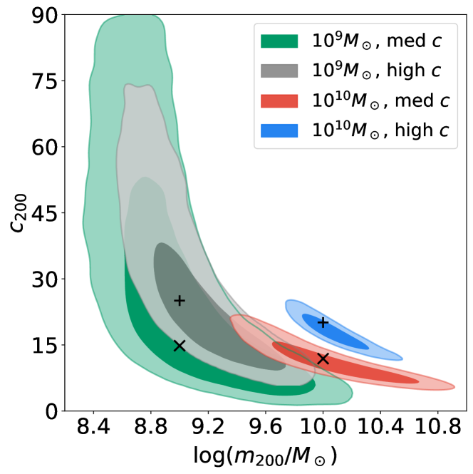
Figure 2.— Joint posteriors in log-mass $\log(m_{200}/M_{\odot})$ and concentration $c_{200}$ of perturbing subhalos in four of our mock data fits at HST resolution and $z_{lens}=0.2$. Green and grey contours represent posteriors for $10^{9}M_{\odot}$ subhalos with concentrations at the median value $\bar{c}(M,z)$ and 2$\sigma$ above the median, respectively; red and blue contours represent $10^{10}M_{\odot}$ subhalos, again at the median and 2$\sigma$ above the median respectively. The ‘x’ markers denote the “true” values for these parameters for the median concentration cases, while the ‘+’ markers denote the true values for the high concentration cases.

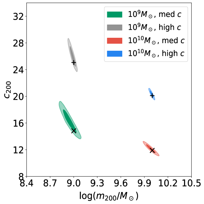
Figure 3.— Joint posteriors in log-mass $\log(m_{200}/M_{\odot})$ and concentration $c_{200}$ of $10^{8}M_{\odot}$ and $10^{9}M_{\odot}$ perturbing subhalos, inferred using high-resolution simulated images with pixel size $\sim 0.01^{\prime\prime}$ and PSF width equal to twice the pixel size. Green and grey contours represent posteriors for $10^{8}M_{\odot}$ subhalos with concentrations at 2$\sigma$ below the median value $\bar{c}(M,z)$ and equal to the median value, respectively; red and blue contours represent $10^{9}M_{\odot}$ subhalos, again at 2$\sigma$ below the median and at the median respectively. The ‘x’ markers denote the “true” values for these parameters for the median concentration cases, while the ‘+’ markers denote the true values for the high concentration cases.

In all modeling runs, the mass is allowed to vary from $10^{6}M_{\odot}-10^{11}M_{\odot}$ and is parameterized as $\log m_{200}$ with a uniform prior over this range (this is equivalent to assuming a logarithmic prior in the subhalo’s mass). We use $\log(m_{200}/M_{\odot})$ as our parameter to allow for better initial coverage of the parameter space during the nested sampling, since the subhalo mass ranges over several orders of magnitude during the fit. When varying the concentration, we use $c_{200}$ as our parameter directly with a logarithmic prior in this parameter covering the range (0.5,100). The host galaxy is modeled with an ellipsoidal power law profile, where all parameters are varied: $b$, $\alpha$, $q$, $\theta$, $x_{c}$ and $y_{c}$ (the Einstein radius, density log-slope, axis ratio, orientation angle, and center coordinates respectively).

3. Constraints on subhalo concentration and mass

3.1. Mass-concentration constraints at HST resolution

Since most $10^{9}M_{\odot}$ subhalos and all $10^{10}M_{\odot}$ subhalos are detected with high significance in our modeling runs, we now investigate the resulting constraints in both mass and concentration for some representative cases. In Figure 2 we plot joint posteriors in $\log(m_{200}/M_{\odot})$ and $c_{200}$ for subhalos at $z_{lens}=0.2$ placed at the closest point to the critical curve (just $0.01^{\prime\prime}$ outside the unperturbed critical curve), for the “large” source galaxy cases. Posteriors are plotted for $10^{9}M_{\odot}$ and $10^{10}M_{\odot}$ subhalos with concentrations at the median value $\bar{c}(M,z)$ and 2$\sigma$ above the median in each case.

In all cases, a degeneracy exists between mass and concentration, since a perturbation of similar size can be produced by increasing the mass while decreasing the concentration, or vice versa (this relationship will be explored in detail in Section 5). Although the constraints on concentration are weak for $10^{9}M_{\odot}$ subhalos, there is nevertheless a lower bound on concentration, and this was generally true for all of the fits that satisfy our detection criterion (Section 2). Nevertheless, impressive constraints on the concentration can be obtained for $10^{10}M_{\odot}$ subhalos. In the median concentration case for which $c_{true}=11.9$, we infer a 50th percentile value $c_{fit}=14.9_{-5.8}^{+8.1}$ where the uncertainties give the 95% credible interval. For the high concentration case where $c_{true}=20.1$, we infer $c_{fit}=22.3_{-4.5}^{+5.6}$. Remarkably, these uncertainties are smaller than the expected 2$\sigma$ scatter in concentration for $10^{10}M_{\odot}$ halos. In principle, it follows that even with a small number of such detections at HST resolution, one may be able to distinguish between the mass-concentration relation expected in CDM (for subhalos) versus alternate scenarios such as warm or self-interacting dark matter (if one assumes the standard power-law spectrum of inflationary perturbations).

All of the cases shown in Figure 2 are for subhalos whose projected position is just outside the critical curve (by $0.01^{\prime\prime}$). To investigate the constraints for subhalos further away from the critical curve, in Figure 5 we plot the resulting constraints for a high-concentration $10^{10}M_{\odot}$ subhalo at different positions: the grey contours correspond to a subhalo at the innermost position, $0.13^{\prime\prime}$ inside the critical curve; red contours are for a subhalo close to the critical curve (same as blue contours in Figure 2); blue contours are for a subhalo at the outermost position, $0.15^{\prime\prime}$ outside the critical curve. Interestingly, the constraints for the outermost subhalo (blue) are nearly as good compared to the subhalo close to the critical curve, whereas the uncertainties are significantly weaker for the innermost subhalo. Nevertheless, significant constraints are obtained in each of these cases.

3.2. Mass-concentration constraints at high resolution

Although the constraints on concentration are weak for $\lesssim 10^{9}M_{\odot}$ subhalos at HST resolution, we can ask whether better constraints will be possible for higher resolutions, e.g. using long baseline interferometry or next-generation very large telescopes. To investigate this, we simulate lenses similar to those shown in Figure 2, but with $10^{8}M_{\odot}$ and $10^{9}M_{\odot}$ subhalos, imaged with pixels four times smaller than HST ($\sim 0.013^{\prime\prime}$ compared to $\sim 0.049^{\prime\prime}$ for HST) and assuming a Gaussian PSF whose width is twice the pixel size. Note that both the Thirty Meter Telescope and Giant Magellan Telescope will exceed this resolution; in principle the ALMA radio telescope array can reach this resolution at long baseline, although the pixel noise is highly correlated due to the interferometry.

The high-resolution constraints on concentration and mass are shown in Figure 3. Remarkably, at this resolution the concentration for $10^{9}M_{\odot}$ subhalos can be well constrained even for low concentrations. At median concentration with $c_{true}=14.83$, we infer $c_{fit}=15.78_{-2.08}^{+2.31}$, much smaller than the expected scatter in concentration at this mass for $\Lambda$CDM. Even more remarkably, meaningful constraints are obtained for $10^{8}M_{\odot}$ even at median or low concentrations whereas neither of these subhalos were even detected to high significance at the HST resolution (in fact the low-concentration perturbation was not detected at all). The latter results should be interpreted with some caution, since it is possible that if the source model is allowed more freedom than in our model (e.g. for pixellated sources), perturbations as small as $10^{8}M_{\odot}$ might be at least partially absorbed into the reconstructed source, possibly weakening the constraints; as pixellated source inversions are computationally intensive, we do not investigate this possibility here. Nevertheless, we conclude that significant constraints on the mass-concentration of perturbing subhalos, possibly down to $10^{8}M_{\odot}$, will be possible for next generation telescopes that attain resolutions $\sim 0.01^{\prime\prime}$ or better.

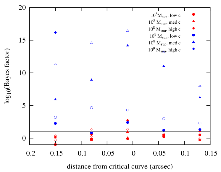
Figure 4.— Log-Bayes factors $\log_{10}K$ versus distance from the critical curve for the subset of mock data at $z_{lens}=0.2$, shown up to $\log_{10}K=20$ (all $10^{10}M_{\odot}$ subhalos exceed this range and therefore are not shown). The black line represents the threshold for which we consider a subhalo “detection” to have occurred, corresponding to $\log_{10}K\gtrsim 1$. Filled markers denote the lenses for which the “small” source galaxy is being lensed, while open markers correspond to the “large” source being lensed (with unlensed widths given by $0.03^{\prime\prime}$ and $0.06^{\prime\prime}$ respectively). The distances are measured from the nearest point on the unperturbed critical curve, with negative values lying outside the critical curve and vice versa.

4. Detections

To examine which subhalo perturbations are actually detectable, in Figure 4 we plot the logarithm of the Bayes factor, $\log_{10}K$, against the subhalo distance from the (unperturbed) critical curve for a subset of lenses from our mock data runs. The dashed line represents our detection criterion, namely $\log K>1$; all cases where $\log K$ is greater than 20 are not shown in the plot (this includes all subhalos with mass $10^{10}M_{\odot}$). Red markers denote $10^{8}M_{\odot}$ subhalos, while blue markers denote $10^{9}M_{\odot}$ subhalos. We only show the subset of concentrations with $\Delta_{c}=(-2,0,2)$, (i.e. 2$\sigma$ below the median, at the median, or 2$\sigma$ above the median); these are denoted by circles, triangles, and diamonds respectively. Filled markers denote lenses generated using the “small” source galaxy, while open markers correspond to the “large” source galaxy.

Note that nearly all $10^{9}M_{\odot}$ subhalos are unambiguously detected, with the exception of the low-concentration subhalos with small sources—these hover near the threshold of detectability, unless very close to the critical curve. This does not mean that the subhalo does not perturb these small sources noticeably (it certainly does), but rather the perturbation is small enough that it can be degenerate with the parameters governing the primary lens. In addition, because the primary lens parameters are less well constrained with the small source, there is more freedom to vary them and possibly mimic the subhalo perturbation. However, we can conclude that all $10^{9}M_{\odot}$ perturbations with large sources and/or concentrations at or above the median are apparently detectable at HST resolutions, at least if they lie within $\sim 0.1$” from the critical curve. One important caveat should be given here, however: for the fits in this section, the source was modeled as a Gaussian without Fourier modes. If more freedom is allowed to the source (e.g. with Fourier modes, or with a pixellated source), it is possible that a few of these cases may be well-modeled without a subhalo, since the perturbation may be absorbed into the source itself while still achieving a good fit.

For $10^{8}M_{\odot}$ the story is very different: at most a few subhalos were unambigiuously detected, with the clearest detection occurring when the subhalo has a high concentration, is perturbing a small source, and is very close to the critical curve. In general, the smaller source galaxy is more favorable for detection due to the small size of the perturbation: a rapid variation in surface brightness is required for the perturbation to be noticeable at all, unless the concentration is quite high (as the open diamonds show). We conclude that relatively few (if any) $10^{8}M_{\odot}$ subhalos will be detected at HST resolutions in CDM, and those that are detected are very likely to have high concentrations; again however, it is possible that with a more flexible source model, even these cases may be well-modeled without a subhalo.

At the higher lens redshift, $z_{lens}=0.5$, the results are essentially the same, hence we omit the figure for this case. We note however that most of the Bayesian evidences are slightly lower compared to $z_{lens}=0.2$. Indeed, nearly all of the subhalo perturbations are less pronounced at higher redshift, due to the fact that the angular size of the NFW scale radius is smaller at higher redshift. Since the ratio of angular diameter distances $D_{lens}(z=0.5)/D_{lens}(z=0.2)\approx 0.5$, the scale radius at the higher redshift appears smaller by nearly this factor (although not precisely, since halos have lower concentrations at higher redshift). Thus the noticeable extent of a subhalo’s perturbation is smaller at high redshift, at least for a primary lens of fixed Einstein radius. As a result, none of the $10^{8}M_{\odot}$ subhalos were unambiguously detected at $z_{lens}=0.5$, even if placed very close to the critical curve. Nevertheless, nearly all $10^{9}M_{\odot}$ subhalos are detected, with the exception of the low-concentration + small source cases with subhalo placed at the extreme positions inside or outside the critical curve.

These results imply that with HST-like resolution, perturbing subhalos of mass $<10^{9}M_{\odot}$ are more likely to be detected if they have a concentration at or above the median expected value for $\Lambda$CDM. For $\sim 10^{8}M_{\odot}$ subhalos, only high-concentration subhalos have a chance to be detected, and only if they are quite close to the critical curve; for $z_{lens}\gtrsim 0.5$, detection of such low-mass subhalos is unlikely in any configuration.

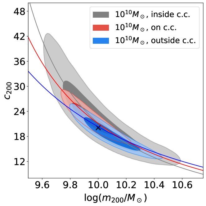
Figure 5.— Joint posteriors for a $10^{10}M_{\odot}$ perturbing subhalo, at different projected positions with respect to the critical curve (and $z_{lens}=0.2$). Grey, red and blue contours correspond to subhalos located $0.13^{\prime\prime}$ inside, $0.01^{\prime\prime}$ outside, and $0.15^{\prime\prime}$ outside the critical curve respectively. The ‘x’ marks the true values for these parameters. The solid curves represent the set of points ($\log(m_{200})$,$c_{200}$) for which the subhalo contains the same projected mass within the perturbation radius $r_{\delta c}$ of the best-fit model in each case.

5. Physical interpretation of the degeneracy between concentration and mass

Note that the correlation in the inferred concentration versus mass is slightly different in the posteriors for each subhalo position in Figure 5, with noticeably different “tilt”. What determines this correlation? In Minor et al. (2017) we showed that for subhalo perturbations, a characteristic perturbation radius can be defined, within which the subhalo’s projected mass is determined robustly, provided the log-slope of the primary galaxy’s density profile is also well-determined. This subhalo perturbation radius $r_{\delta c}$ is defined as the projected distance from the subhalo’s center to the point where the critical curve is perturbed the most, and to good approximation typically lies along the line from the primary galaxy’s center to the position of the subhalo. To check whether this mass is robustly determined for the $10^{10}M_{\odot}$ case plotted here, we used the following procedure: first, we calculated $r_{\delta c}$ for the best-fit model in each case, and the corresponding mass within this radius; next, for an array of $m_{200}$ values over the range of the posteriors, we calculated what concentration is required to keep the mass within $r_{\delta c}$ constant, using a numerical root finder. The resulting curves are plotted in Figure 5, with colors matching the corresponding posterior. Note that the overall correlation is recovered very well, indicating the perturbation radius is well constrained; the tilts differ because the inferred $r_{\delta c}$ is different in each case, due to the differing subhalo positions.

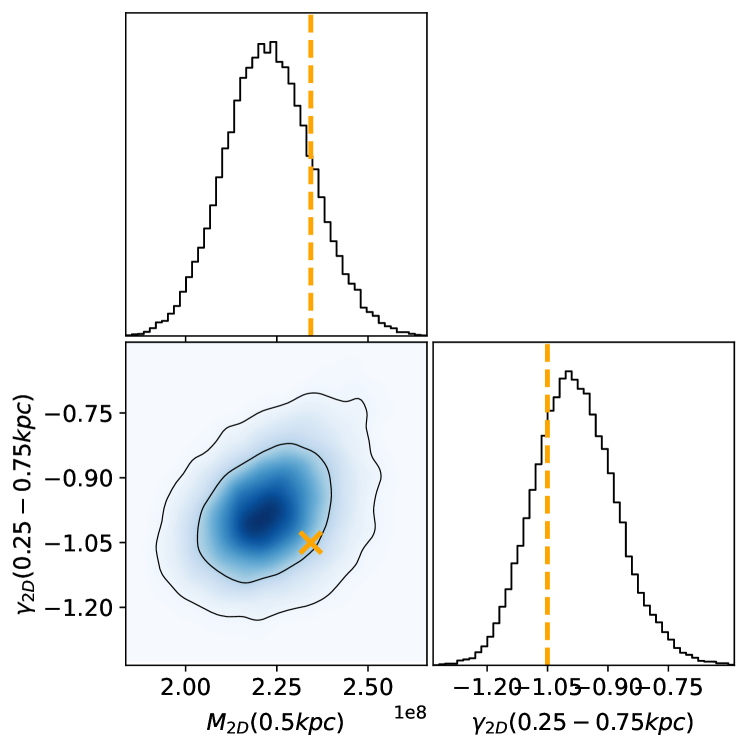
Figure 6.— Joint posterior in the projected subhalo mass within 0.5 kpc, $M_{2D}($0.5kpc$)$, versus the average log-slope of the density profile from 0.25 to 0.75 kpc, $\gamma_{2D}($0.25-0.75kpc$)$. The mock data was produced with a perturbing subhalo of mass $m_{200}=10^{10}M_{\odot}$ and concentration 2$\sigma$ above the median CDM value, whose posterior in $m_{200}$ and $c_{200}$ is shown as the blue contour in Figure 2. After fitting the mock data, the subhalo’s inferred perturbation radius $r_{\delta c}\approx$ 0.5 kpc, so we choose the projected mass and log-slope around this radius as our derived parameters. The actual parameter values are given by the orange marker. Note that, unlike $m_{200}$ and $c_{200}$, there is no significant degeneracy between these two parameters and the mass is well-constrained to within $\approx 10\%$.

Since the subhalo’s projected mass within the perturbation radius can be determined robustly, another way to cast the results is to infer a derived parameter $M_{2D}(r_{\delta c,bf})$ where $r_{\delta c,bf}$ is the approximate best-fit perturbation radius from the fit. Likewise, as a proxy for concentration, one can define a derived parameter $\gamma_{2D}$ as the average density log-slope in the vicinity of the perturbation radius, since this is the region where the subhalo’s perturbation should yield the most information about the profile. For example, in Figure 6 we plot joint posteriors for the perturbing subhalo of mass $m_{200}=10^{10}M_{\odot}$ and concentration $2\sigma$ above the median CDM value (whose posterior in $m_{200}$ and $c_{200}$ is shown as the blue contour in Figure 2). For this subhalo, the best-fit perturbation radius $r_{\delta c}\approx 0.5^{\prime\prime}$, so we choose this radius to evaluate $M_{2D}($0.5kpc$)$. We likewise define the average log-slope of the density profile from 0.25 to 0.75, $\gamma_{2D}(0.25-0.75$kpc$)$. Note that there is almost no discernible degeneracy between these two parameters, and $M_{2D}$ is well-constrained to within $\approx 10\%$. These inferences can be compared to dark matter simulations provided the simulation resolution is sufficiently high. Note that, unlike $M_{2D}$, there is no guarantee that the inferred log-slope will be independent of the subhalo profile chosen; its robustness may depend on the actual interval chosen for evaluating the slope. Nevertheless, the advantage of switching to log-slope is that it is more straightforward to compare to simulations and among different lensing solutions, as it does not depend on defining a theoretical $r_{200}$ or $m_{200}$ for a subhalo. In a companion paper (Minor et al. 2020, in prep), we use exactly this approach when modeling the subhalo detected in the gravitational lens SDSSJ0946+1006 (Vegetti et al., 2010).

Although we have explained how the degeneracy between subhalo mass and concentration arises, we must still understand what determines the inferred limits on the concentration. In Section 7 we will investigate what is physically constraining the subhalo concentration at the high and low ends, and whether tidal truncation significantly alters these constraints.

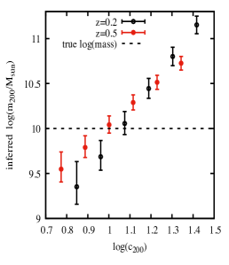
(a) $10^{10}M_{\odot}$ subhalo

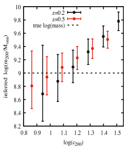
(b) $10^{9}M_{\odot}$ subhalo

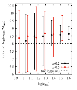
(c) $10^{8}M_{\odot}$ subhalo

Figure 7.— Inferred subhalo mass $m_{200}$ plotted against the subhalo’s actual (log) concentration $c_{200}$, where the modeling assumes the subhalo’s concentration to be at the median value for $\Lambda$CDM during the fit. Black (red) points show the 50th percentile inferred value for $m_{200}$ for lenses at $z_{lens}=0.2$ ($z_{lens}=0.5$), while error bars show the 95% credible intervals. Dashed line shows the subhalo’s true mass in each case. The log-concentrations chosen for the mock data (horizontal axis) differ from the median value $\log\bar{c}(M,z)$ by (-2$\sigma$, -1$\sigma$, 0, 1$\sigma$, 2$\sigma$, 3$\sigma$) where $\sigma\approx 0.11$ is the scatter in concentration observed in $\Lambda$CDM simulations.

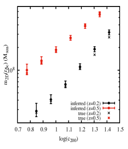
(a) robust mass, $10^{10}M_{\odot}$

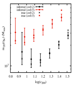
(b) robust mass, $10^{9}M_{\odot}$

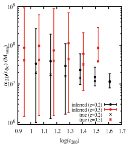
(c) robust mass, $10^{8}M_{\odot}$

Figure 8.— Constraint on the subhalo’s projected mass enclosed within its perturbation radius $r_{\delta c}$, plotted against the subhalo’s actual (log) concentration $c_{200}$ where the modeling assumes the concentration to be at the median value for $\Lambda$CDM during the fit. Plotting conventions are the same as in Figure 7, except that the corresponding true values $M_{2D,true}$ are plotted with a black ‘x’ for $z=0.2$, and a red asterisk for $z=0.5$.

6. Can scatter in the mass-concentration relation be ignored when modeling subhalo perturbations?

6.1. Bias in the inferred subhalo mass

Several recent lens modeling studies have modeled subhalo perturbations using an NFW profile, under the assumption that the concentration takes on the median value for $\Lambda$CDM, ignoring the expected scatter in subhalo concentrations (Despali et al., 2018; Ritondale et al., 2019; Li et al., 2017). However, Figure 2 already suggests that the effect can be substantial: for example, if a $10^{10}M_{\odot}$ subhalo has a concentration 2$\sigma$ above the median (the rightmost ‘x’ in the figure), but one assumes that it has a median concentration (which is a factor of $\sim$1.7 smaller), the inferred mass indicated by the posterior will be substantially larger. The reason is straightforward: if one underestimates the concentration, then more mass is required to generate a sufficiently large perturbation (this is discussed in detail in Section 5).

Here we investigate to what extent the inferred mass of a subhalo can be biased due to scatter in concentration, if one assumes the subhalo’s concentration is determined by the median value $\bar{c}(M,z)$ expected in $\Lambda$CDM. We model all of the mock data described in Section 2.2, varying the subhalo’s position and $\log(m_{200})$ parameters while keeping the concentration set to $\bar{c}(m_{200},z_{lens})$ during the fit.

In Figure 7 we plot the inferred subhalo mass $m_{200}$ versus the subhalo’s actual concentration (or rather, log-concentration) for each of the subhalo masses in our mock data grid ($10^{10}M_{\odot}$, $10^{9}M_{\odot}$, $10^{8}M_{\odot}$ correspond to 7(a), 7(b), 7(c) respectively). The circles show the 50th percentile inferred values, while the error bars show the 95% credible interval; black bars are for $z_{lens}=0.2$, while red bars are for $z_{lens}=0.5$. In each subplot, recall that the actual concentrations range from being -2$\sigma$ below the median value, all the way up to 3$\sigma$ above the median value, with the third bar from the left corresponding to subhalos at the median concentration. The subhalo was located near the critical curve (at $0.01^{\prime\prime}$ outside) for all the cases plotted. For $10^{10}M_{\odot}$ and $10^{9}M_{\odot}$, the “large” source galaxy was used since the uncertainties are somewhat smaller in these cases, whereas for $10^{8}M_{\odot}$, the small source was used since a greater number of detections occurred in this case.

In Figure 7(a), one can see that for lenses at $z=0.2$, $10^{10}M_{\odot}$ subhalos that are 1$\sigma$ above the median have an inferred mass that is biased high by nearly a factor of 3, while subhalos 1$\sigma$ below the median are biased low by a factor of $\sim$2. At 2$\sigma$ the bias is even more severe, roughly a factor of $\sim$6. The corresponding bias at $z=0.5$ is somewhat smaller, roughly half as large (a factor of $\sim$3) for concentrations $2\sigma$ above the median; this pattern is similar for the $10^{9}M_{\odot}$ case. For $10^{9}M_{\odot}$ perturbers (Figure 7(b)) the bias is not as severe, but nevertheless $m_{200}$ is biased by a factor of $\sim$2 for subhalos whose concentrations are 1$\sigma$ above the median, and between 3-4 for subhalos 2$\sigma$ above the median. For $10^{8}M_{\odot}$, only the subhalos above the median concentration were detected at all; in these cases however, we see bias of roughly a factor of 3, albeit with large uncertainties.

Although one might expect that very few subhalos ($\sim$5%) would happen to have concentrations 2$\sigma$ away from the median, and hence the mass is unlikely to be biased by a factor greater than 2, this may not be the case, for two reasons. 1) Subhalos tend to have systematically higher concentrations than field halos, as a result of tidal interactions with the host galaxy; hence, a greater proportion of subhalos at high concentration is likely. 2) For subhalos of mass $\lesssim 10^{9}M_{\odot}$, high-significance detections are more likely to occur for subhalos whose concentrations are above the median value. Thus, even in $\Lambda$CDM one may expect that the inferred subhalo mass may be biased significantly in many cases, possibly up to a factor of 6, if scatter in concentration is neglected when modeling lenses.

Finally, an additional source of bias in the inferred perturber mass comes from the fact that many perturbing halos may actually be unassociated halos along the line-of-sight to the lens, rather than subhalos (Xu et al., 2012; Li et al., 2017; Çaǧan Şengül et al., 2020). If the redshift of the perturber differs significantly from the redshift of the primary lens, this may bias the inferred halo mass if unaccounted for during the lens modeling (Despali et al., 2018). In principle this bias can be quantified using the same methodology in this paper, with a corresponding redshift scaling of the inferred mass (especially the projected mass $M_{2D}(r_{\delta c})$) depending on the unknown perturber redshift. We leave this analysis to future work.

6.2. Testing the robust subhalo mass estimator

If subhalos are indeed well-approximated by a spherical NFW profile with only modest tidal truncation in most cases, then a straightforward way to overcome the bias in the inferred mass is to vary both the mass and concentration as free parameters. In fact, we have seen in Section 3.1 that this approach can yield important constraints about the concentration itself. Nevertheless, it is useful to have a mass estimate that is robust even if the assumed density profile is incorrect (e.g. due to incorrect assumptions about the concentration, tidal radius, or log-slope). In Minor et al. (2017) we showed that a robust mass can be defined in terms of the projected mass contained within the subhalo’s perturbation radius $r_{\delta c}$. However, this robust mass estimator was tested using a simulated version of the ALMA lens SDP.81 for which the perturbation radius was very well-constrained; this is not always the case for many of our simulated lenses at HST resolutions with low-mass or low-concentration perturbations.

Thus, it is useful to test whether this mass estimator—the projected mass enclosed within the perturbation radius—is indeed unbiased for the subhalo fits shown in Figure 7. To do this, we carry out the following procedure: 1) Calculate the perturbation radius $r_{\delta c}$ as a derived parameter during the nested sampling run. 2) After the run is finished, choose the median (50th percentile) inferred value of $r_{\delta c}$, which we call $r_{\delta c,fit}$ (one could also use the best-fit point for this). 3) For each point in the chain, calculate the subhalo’s projected mass enclosed within the radius $r_{\delta c,fit}$, which we call $M_{2D,fit}\equiv M_{2D}(r_{\delta c,fit})$; this will be our mass estimator. 4) Plot the resulting posterior in $M_{2D,fit}$ and compare this to the actual projected mass within the same radius, which we call $M_{2D,true}$. The latter point is important, since the true perturbation radius may differ from our inferred value.

The results of this procedure are shown in Figure 8. The conventions are similar to Figure 7, except now we are plotting the mass $M_{2D,fit}$ and comparing to $M_{2D,true}$ in each case, marked with an ‘x’ for $z=0.2$ (or an asterisk for $z=0.5$). In nearly all cases $M_{2D}$ is recovered fairly well: for the $10^{10}M_{\odot}$ perturber (Figure 8(a)), $M_{2D,fit}$ differs from the true value by less than 20% in all cases; the same is true for the $10^{9}M_{\odot}$ and $10^{8}M_{\odot}$ perturbers except for the lowest-concentration case, for which the bias is 26-27% (albeit still within the error bars). In all cases, the bias in the subhalo’s total inferred mass is substantially larger. For example, the $10^{9}M_{\odot}$ perturber with median concentration infers $M_{2D}$ with a bias of 8%, whereas the total inferred mass $m_{200}$ is biased by 123% (over a factor of 2). The numbers become starker for higher concentrations: for the cases with concentrations 2$\sigma$ above the median value, $M_{2D}$ is biased by a factor of 1.18, 0.90, and 0.99 for $\log m_{200}$ = 10, 9, and 8 respectively; the corresponding bias factors in $m_{200}$ are 6.3, 3.6, and 2.6. As expected, the bias in $M_{2D}$ was greatest in the cases for which the inferred perturbation radius $r_{\delta c}$ differed the most from its true value. However, even in cases where the true $r_{\delta c}$ lay outside the 95% probability region, the inferred $M_{2D,fit}$ was biased by less than 20%.

We conclude that the mass estimator from Minor et al. (2017) is indeed robust, even at HST resolutions where the perturbation radius may be comparable to the pixel size, provided one follows the procedure outlined above. More generally, it has the additional advantage of providing physical insight into what is really being constrained during the lensing, as Section 5 demonstrates. The perturbation radius can be calculated numerically via a standard root-finding algorithm; for details we refer the reader to Section 7.3 of Minor et al. (2017). In this way, $r_{\delta c}$ (and the corresponding subhalo mass enclosed within it) can be incorporated into existing lensing codes if desired and calculated as a derived parameter during lens modeling.

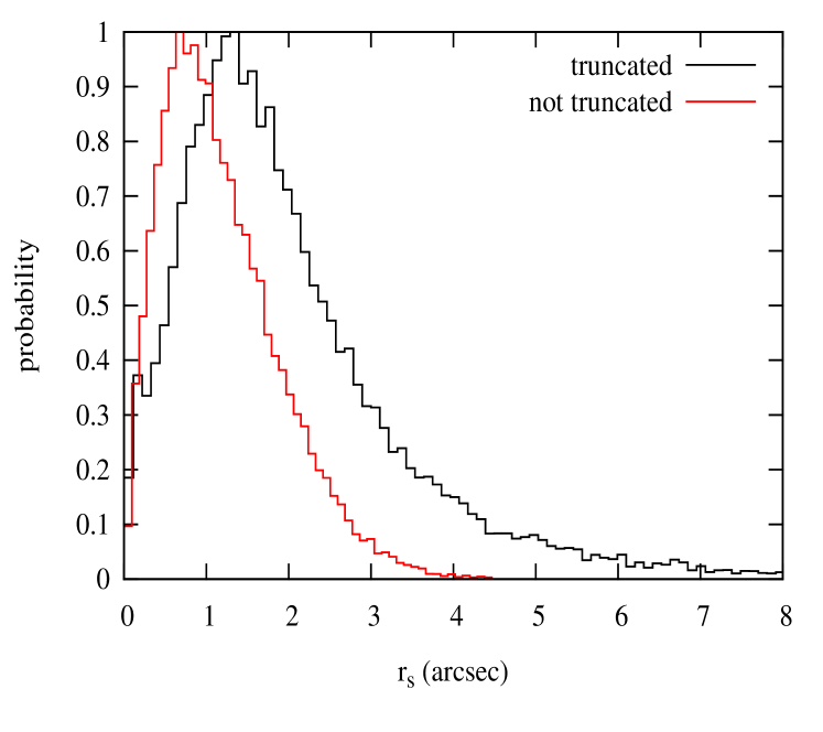
Figure 9.— Derived posteriors in the NFW scale radius $r_{s}$ of a $10^{10}M_{\odot}$ perturber at $z=0.2$. Black curve corresponds to a severely truncated subhalo with truncation radius $r_{t}\approx 0.29^{\prime\prime}$, which was modeled with $r_{t}$ fixed to this value. Red curve corresponds to a non-truncated $10^{10}M_{\odot}$ subhalo that generates a perturbation with the same scale $r_{\delta c}\approx 0.058^{\prime\prime}$. Note that for the truncated subhalo, $r_{s}$ is allowed to be quite large (and hence, low $c_{200}$) because the perturbation is suppressed outside the truncation radius. For most subhalos $r_{t}$ will be much greater than $r_{\delta c}$, so significant lower bounds on $c_{200}$ can be obtained.

7. Discussion: What really constrains the subhalo concentration?

In Section 5 we have shown that the correlation between the inferred subhalo mass and subhalo concentration seen in sufficiently large perturbations (Figures 2, 3) can be explained in terms of the mass enclosed within the perturbation radius being an approximately conserved quantity. However this cannot be the only physical constraint of interest, because it does not explain the upper/lower bounds on the inferred concentration. Here, we discuss the origin of the constraints on the subhalo concentration.

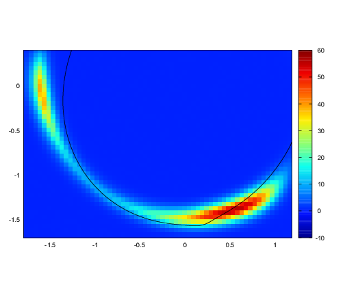
(a) $c=2$   $(m_{200}\approx 2.4\times 10^{12}M_{\odot})$

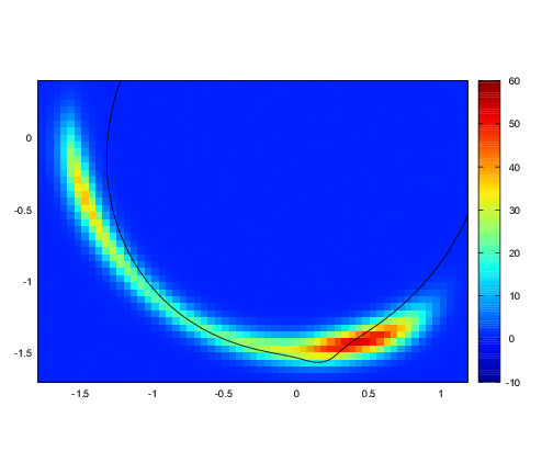
(b) $c=10$   $(m_{200}\approx 5.0\times 10^{10}M_{\odot})$

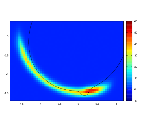
(c) $c=40$   $(m_{200}\approx 3.0\times 10^{9}M_{\odot})$

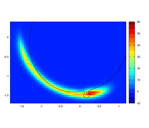
(d) $c=160$   $(m_{200}\approx 8.2\times 10^{8}M_{\odot})$

Figure 10.— Comparison of the image perturbation produced by a subhalo with perturbation radius $r_{\delta c}=0.14^{\prime\prime}$, for four different concentrations: $c=2,10,40,160$. For each concentration, the subhalo mass $m_{200}$ is adjusted to produce the same $r_{\delta c}$. Note that for low concentrations ($c=2,10$), the images are perturbed far beyond the perturbation radius, whereas for high concentrations ($c=40,160$) only the immediate vicinity of the perturbation (up to a few times the perturbation radius) is affected. For reference, the perturbation size $r_{\delta c}=0.14^{\prime\prime}$ is the same as that produced by a $10^{10}M_{\odot}$ subhalo at the same location, with concentration $2\sigma$ above the median (blue contour in Figure 2).

In general, all of the subhalos that were detected in our mock data, no matter how small, produced a lower bound on the inferred concentration. This is the case even for $10^{8}M_{\odot}$ and low-concentration $10^{9}M_{\odot}$ subhalos for which the perturbation radius $r_{\delta c}$ is comparable to the pixel size, and hence is not well constrained. This indicates that the lower bound is not coming from the immediate neighborhood of the critical curve perturbation, but further out in the lens plane. Indeed, for sufficiently low concentrations, the images are visibly perturbed well beyond $r_{\delta c}$. This can be seen in Figure 10, where a subhalo with a perturbation radius $r_{\delta c}=0.14^{\prime\prime}$ is shown with different concentrations (this is the same $r_{\delta c}$ produced by a $10^{10}M_{\odot}$ subhalo with concentration $2\sigma$ above median, which corresponds to the blue contour in Figure 2). We plot the resulting images for $c=2,10,40,160$; note that the subhalo’s $m_{200}$ is different in each figure, in order to produce the same $r_{\delta c}$ in each case. If the subhalo has too low of a concentration ($c=2,10$ in panels (a) and (b) respectively), the surface brightness far outside the perturbation radius is affected, as well as the overall size of the critical curve itself. To some extent, this can be compensated for by adjusting the primary lens parameters, in particular the Einstein radius and center coordinates, as well as the source galaxy parameters. However, for low enough concentrations, the subhalo mass must be very large to reproduce the critical curve perturbation scale, and adjusting the primary lens/source parameters is not enough to achieve a good fit.

To demonstrate this, we can simulate and model a perturbation where the subhalo is severely truncated, forcing the perturbation to be more local. We generated a mock image using a truncated NFW profile for a $m_{200}=10^{10}M_{\odot}$ (note this is the virial mass in the absence of truncation) with median concentration, and setting the truncation radius $r_{t}$ to be roughly 5 times the perturbation radius ($r_{t}\approx 0.29^{\prime\prime}$, $r_{\delta c}\approx 0.058^{\prime\prime}$). We then fit a subhalo with the truncation radius fixed to the correct value, thus forcing the perturbation to be small outside this region. In Figure 9 we plot the posterior probability in the NFW scale radius $r_{s}$, which is a derived parameter, where the black curve denotes the truncated fit. The red curve denotes the probability for an untruncated $10^{10}M_{\odot}$ subhalo, modeled without truncation, for comparison. The furthest image from the subhalo is approximately 2 arcseconds away, and this is roughly the limit on $r_{s}$ for the non-truncated subhalo. However the scale radius is allowed to be significantly larger (and thus, lower $c_{200}$) for the truncated subhalo, since the truncation prevents the perturbation from extending far beyond $r_{t}$. In reality, subhalos are unlikely to be tidally stripped far within $r_{s}$ without being disrupted altogether. In cases where $r_{t}\gtrsim r_{s}$, the truncation does not significantly affect the lower bound on $c_{200}$.

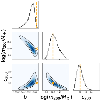
Figure 11.— Joint posteriors for a lens at $z=0.2$ perturbed by a subhalo at that is truncated at $r_{max}\approx 2.16r_{s}$, fit by an NFW profile without truncation. The parameters shown are the host galaxy Einstein radius $b$, subhalo log-mass $\log(m_{200})$, and subhalo concentration $c_{200}$. Note that the inferred subhalo mass and concentration are unbiased by the approximation of no truncation, while the host galaxy’s Einstein radius comes out biased slightly low to offset the extra mass beyond the subhalo’s actual tidal radius.

In contrast to the lower limit on $c_{200}$, we find that the concentration on the high-end is only constrained if the perturbation radius is large enough that the shape of the critical curve perturbation can be distinguished. This requires $r_{\delta c}$ to be at least as large as the PSF width (which in our simulations is roughly $0.05^{\prime\prime}$). Such is the case for all $10^{10}M_{\odot}$ subhalos in our mock data, as well as $10^{9}M_{\odot}$ subhalos with concentrations above the median $\Lambda$CDM value (for both $z=0.2$ and $z=0.5$). This can be seen in panels (c) and (d) of Figure 10, where the surface brightness in the vicinity of the perturbation (up to a few times $r_{\delta c}=0.14^{\prime\prime}$) can be distinguished between $c=40$ and $c=160$, allowing for the concentration to be constrained at the high end for this perturbation scale (blue contour in Figure 2). Such is also the case for the subhalo perturbing the lens SDSSJ0946+1006, whose concentration is higher than 3$\sigma$ above the expected median in CDM, generating $r_{\delta c}\sim 0.3^{\prime\prime}$ as we show in a companion paper (Minor et al. 2020, in prep). However, for our mock data with a $10^{9}M_{\odot}$ subhalo with concentration at the median, we have $r_{\delta c}\approx 0.05^{\prime\prime}$ and there is no significant upper bound on the inferred concentration from the data, as can be seen in Figure 2 (green contour). When the resolution is increased, as in Figure 3, the perturbation is better resolved so that $c_{200}$ is constrained even for a low-concentration $10^{9}M_{\odot}$ subhalo, while a much stronger upper bound on the concentration is achievable for larger perturbations.

8. Effect of tidal stripping on the inferred mass-concentration of subhalos

We have seen that the concentration of $10^{10}M_{\odot}$ subhalos can be significantly constrained even at HST resolution (Figure 2), while lower mass subhalo concentrations can be constrained at higher resolutions (Figure 3). However, our modeling up to now has ignored tidal stripping of subhalos. Since tidal truncation may mimic the effect of having a higher concentration to some extent, here we test whether the mass-concentration constraints are affected by tidal truncation.

$\Lambda$CDM simulations show that tidal stripping results in subhalos being truncated at or above $r_{max}\approx 2.16r_{s}$, while few subhalos are truncated below $r_{max}$ without severe tidal disruption occurring. Hence, we will simulate a truncated NFW subhalo with tidal radius $r_{t}=r_{max}$ and model it with an NFW profile to see if the resulting $m_{200}$ and $c_{200}$ are biased. For truncated subhalos, we use the following “smoothly truncated” profile from Baltz et al. (2009):

$$\rho(r;r_{s},r_{t})=\frac{\rho_{0}}{\frac{r}{r_{s}}\left(1+\frac{r}{r_{s}}\right)^{2}\left(1+\left(\frac{r}{r_{t}}\right)^{2}\right)^{2}}$$ (4)

where $r_{t}$ is the tidal truncation radius. As our test case, we choose $m_{200}=10^{10}M_{\odot}$ and $c_{200}=\bar{c}(M,z)$, solving for the appropriate $\rho_{0}$ and $r_{s}$ values for an NFW profile. We then truncate the profile using $r_{t}=r_{max}=2.16r_{s}$ and generate simulated data using the same procedure as in 2. The effect of truncation on the images is small within the perturbation radius, but quite noticeable outside it; the images near the critical curve are reduced slightly, while the farthest (and least magnified) image is displaced inwards roughly by one pixel-length. In addition, the critical curve as a whole is slightly smaller. This begs the question whether subhalo inferences can be significantly biased by fitting a tidally stripped subhalo with an NFW profile without truncation.

To answer this, we fit this mock image assuming an NFW subhalo as in Section 2. Posteriors in $m_{200}$, $c_{200}$ and host galaxy Einstein radius $b$ are shown in Figure 11. Remarkably, there is no apparent bias in $m_{200}$ and $c_{200}$, despite completely ignoring the tidal truncation; however, the Einstein radius of the primary lens is biased low, in order to reduce the size of the critical curve in the absence of tidal truncation. This is accompanied by a simultaneous slight adjustment of the width and ellipticity of the source galaxy. One can see that in the limit of high concentration and low mass (approximating a truncated subhalo, in a rough sense), the Einstein radius approaches its actual value; in this limit however, the shape of the critical curve perturbation is noticeably altered in the vicinity of the perturbation radius (becoming “sharper” in appearance), degrading the fit. Hence, the best fit is achieved when the primary lens parameters are slightly adjusted, with the result that there is no discernible bias in the inferred subhalo concentration or mass parameters.

From this, we can conclude that tidal truncation is not expected to significantly bias the inferred subhalo mass for perturbers with CDM-like concentrations, at least at HST resolution. Nevertheless, it is possible that for high concentration perturbers, the effect of strong tidal truncation (up to $r_{s}$) is more local and not as easily mimicked by adjusting the primary lens model. For very strong perturbations, it is therefore advisable to include a tidal radius as a model parameter to reduce bias in the inferred subhalo parameters.

9. Conclusions

We have demonstrated that the concentrations of dark matter subhalos perturbing a gravitationally lensed image are an important factor in the strength of the perturbation, allowing for joint constraints on the mass and concentration of subhalos. At HST-like resolutions, we show that the subhalo concentration can be constrained for $\gtrsim 10^{10}M_{\odot}$ subhalos whose concentrations fall within the expected scatter in $\Lambda$CDM (Figure 2); constraints for lower mass subhalos may be possible if their concentrations are higher than the scatter expected in CDM. Looking to the future, we have shown that constraints on perturber concentration are achievable for $\gtrsim 10^{8}M_{\odot}$ subhalos at the $\sim 0.01^{\prime\prime}$ resolution (Figure 3) attainable by long-baseline interferometry and next-generation extremely large telescopes. This will make it possible to constrain the mass-concentration relation of dark matter halos on small scales from strong lensing perturbations. This approach is complementary to testing the expected mass function of $\Lambda$CDM at dwarf galaxy scales and provides a probe of the small-scale matter power spectrum in addition to dark matter physics.

Likewise, the concentration of perturbers plays an important role in the detectability of the perturbation. We have modeled a large number of mock lenses at HST resolution with subhalo perturbations involving a variety of masses and concentrations, in each case fitting a model with versus without a subhalo. For subhalos with masses of $10^{8}M_{\odot}$, the Bayesian evidence strongly favors a subhalo only if the subhalo is quite close to the critical curve and if the concentration is at least $2\sigma$ above the expected median value in $\Lambda$CDM, indicating only the most concentrated $10^{8}M_{\odot}$ subhalos are likely to have detectable perturbations. For $10^{9}M_{\odot}$ subhalos, we find that perturbations are detectable over a broad range of positions (by the same criterion) only if their concentrations are at or above the median value in $\Lambda$CDM. In general, we conclude that perturbing subhalos of mass $<10^{9}M_{\odot}$ may not be detected unless they have concentrations above the median expected value for $\Lambda$CDM.

We have also shown that if scatter in the mass-concentration relation is unaccounted for during lens modeling, the inferred subhalo masses can be biased biased by a factor of 3(6) for subhalos of mass $10^{9}M_{\odot}$($10^{10}M_{\odot}$) (Figure 7). This bias can be eliminated in one of two ways: 1) varying both the concentration and mass as free parameters; 2) instead of inferring the total mass, inferring the projected mass within the subhalo’s perturbation radius, defined by its distance to the critical curve of the lens at the point of maximum perturbation. The latter can be determined much more robustly than the total subhalo mass, with little degeneracy with concentration or density slope, as demonstrated in Figure 6. In practice, both strategies can be combined, providing constraints on both $c_{200}$ and $m_{200}$ for perturbing halos under the assumption of an NFW profile, while also providing a robust mass measurement that holds even if the assumed density profile is incorrect (e.g. if a dark matter larger core is present). We use this approach to model the substructure in the lens SDSSJ0946+1006 in a companion paper (Minor et al. 2020, in prep).

Finally, we have shown that for HST resolutions, even strong tidal truncation has a negligible bias on the inferred subhalo parameters for high-mass subhalos with CDM-like concentrations (Figure 11). We caution, however, that the bias may be more significant for highly concentrated perturbers or at higher resolutions; in such cases, the safest approach may be to include tidal truncation as a model parameter for the subhalo.

As next-generation sky surveys and ground-based extremely large telescopes come online, the ability to measure subhalo concentrations will provide a critical test of the cold dark matter paradigm. The resulting constraints, perhaps in concert with other probes, may provide valuable insights into dark matter physics and the small-scale matter power spectrum.

References

- ALMA Partnership et al. (2015) ALMA Partnership, Vlahakis, C., Hunter, T. R., Hodge, J. A., & et al. 2015, ApJ, 808, L4
- Ashoorioon & Krause (2006) Ashoorioon, A. & Krause, A. 2006, ArXiv High Energy Physics - Theory e-prints
- Baltz et al. (2009) Baltz, E. A., Marshall, P., & Oguri, M. 2009, J. Cosmology Astropart. Phys, 1, 015
- Bechtol et al. (2015) Bechtol, K., Drlica-Wagner, A., Balbinot, E., Pieres, A., Simon, J. D., et al. 2015, ApJ, 807, 50
- Bose et al. (2017) Bose, S., Hellwing, W. A., Frenk, C. S., Jenkins, A., Lovell, M. R., Helly, J. C., Li, B., Gonzalez-Perez, V., & Gao, L. 2017, MNRAS, 464, 4520
- Brown et al. (2014) Brown, T. M., Tumlinson, J., Geha, M., Simon, J. D., Vargas, L. C., VandenBerg, D. A., Kirby, E. N., Kalirai, J. S., Avila, R. J., Gennaro, M., Ferguson, H. C., Muñoz, R. R., Guhathakurta, P., & Renzini, A. 2014, ApJ, 796, 91
- Çaǧan Şengül et al. (2020) Çaǧan Şengül, A., Tsang, A., Diaz Rivero, A., Dvorkin, C., Zhu, H.-M., & Seljak, U. 2020, Phys. Rev. D, 102, 063502
- Despali et al. (2018) Despali, G., Vegetti, S., White, S. D. M., Giocoli, C., & van den Bosch, F. C. 2018, MNRAS, 475, 5424
- Dutton & Macciò (2014) Dutton, A. A. & Macciò, A. V. 2014, MNRAS, 441, 3359
- Elbert et al. (2014) Elbert, O. D., Bullock, J. S., Garrison-Kimmel, S., Rocha, M., Oñorbe, J., & Peter, A. H. G. 2014, ArXiv e-prints
- Feng et al. (2009) Feng, J. L., Kaplinghat, M., Tu, H., & Yu, H.-B. 2009, J. Cosmology Astropart. Phys, 2009, 004
- Fitts et al. (2017) Fitts, A., Boylan-Kolchin, M., Elbert, O. D., Bullock, J. S., Hopkins, P. F., Oñorbe, J., Wetzel, A., Wheeler, C., Faucher-Giguère, C.-A., Kereš, D., Skillman, E. D., & Weisz, D. R. 2017, MNRAS, 471, 3547
- Garrison-Kimmel et al. (2014) Garrison-Kimmel, S., Horiuchi, S., Abazajian, K. N., Bullock, J. S., & Kaplinghat, M. 2014, MNRAS, 444, 961
- Gilman et al. (2020) Gilman, D., Du, X., Benson, A., Birrer, S., Nierenberg, A., & Treu, T. 2020, MNRAS, 492, L12
- Green et al. (2004) Green, A. M., Hofmann, S., & Schwarz, D. J. 2004, MNRAS, 353, L23
- Hezaveh et al. (2016) Hezaveh, Y. D., Dalal, N., Marrone, D. P., Mao, Y.-Y., Morningstar, W., Wen, D., Blandford, R. D., Carlstrom, J. E., Fassnacht, C. D., Holder, G. P., Kemball, A., Marshall, P. J., Murray, N., Perreault Levasseur, L., Vieira, J. D., & Wechsler, R. H. 2016, ApJ, 823, 37
- Kobayashi & Takahashi (2011) Kobayashi, T. & Takahashi, F. 2011, J. Cosmology Astropart. Phys, 1, 26
- Li et al. (2017) Li, R., Frenk, C. S., Cole, S., Wang, Q., & Gao, L. 2017, MNRAS, 468, 1426
- Lovell et al. (2014) Lovell, M. R., Frenk, C. S., Eke, V. R., Jenkins, A., Gao, L., & Theuns, T. 2014, MNRAS, 439, 300
- Minor & Kaplinghat (2015) Minor, Q. E. & Kaplinghat, M. 2015, Phys. Rev. D, 91, 063504
- Minor et al. (2017) Minor, Q. E., Kaplinghat, M., & Li, N. 2017, ApJ, 845, 118
- Moliné et al. (2017) Moliné, Á., Sánchez-Conde, M. A., Palomares-Ruiz, S., & Prada, F. 2017, MNRAS, 466, 4974
- Navarro et al. (1996) Navarro, J. F., Frenk, C. S., & White, S. D. M. 1996, ApJ, 462, 563
- Ocvirk et al. (2016) Ocvirk, P., Gillet, N., Shapiro, P. R., Aubert, D., Iliev, I. T., Teyssier, R., Yepes, G., Choi, J.-H., Sullivan, D., Knebe, A., Gottlöber, S., D’Aloisio, A., Park, H., Hoffman, Y., & Stranex, T. 2016, MNRAS, 463, 1462
- Peng et al. (2010) Peng, C. Y., Ho, L. C., Impey, C. D., & Rix, H.-W. 2010, AJ, 139, 2097
- Ritondale et al. (2019) Ritondale, E., Vegetti, S., Despali, G., Auger, M. W., Koopmans, L. V. E., & McKean, J. P. 2019, MNRAS, 485, 2179
- Rocha et al. (2013) Rocha, M., Peter, A. H. G., Bullock, J. S., Kaplinghat, M., Garrison-Kimmel, S., Oñorbe, J., & Moustakas, L. A. 2013, MNRAS, 430, 81
- Sawala et al. (2016) Sawala, T., Frenk, C. S., Fattahi, A., Navarro, J. F., Theuns, T., Bower, R. G., Crain, R. A., Furlong, M., Jenkins, A., Schaller, M., & Schaye, J. 2016, MNRAS, 456, 85
- Suyu et al. (2006) Suyu, S. H., Marshall, P. J., Hobson, M. P., & Blandford, R. D. 2006, MNRAS, 371, 983
- Vegetti & Koopmans (2009) Vegetti, S. & Koopmans, L. V. E. 2009, MNRAS, 392, 945
- Vegetti et al. (2014) Vegetti, S., Koopmans, L. V. E., Auger, M. W., Treu, T., & Bolton, A. S. 2014, MNRAS, 442, 2017
- Vegetti et al. (2010) Vegetti, S., Koopmans, L. V. E., Bolton, A., Treu, T., & Gavazzi, R. 2010, MNRAS, 408, 1969
- Vegetti et al. (2012) Vegetti, S., Lagattuta, D. J., McKean, J. P., Auger, M. W., Fassnacht, C. D., & Koopmans, L. V. E. 2012, Nature, 481, 341
- Xu et al. (2012) Xu, D. D., Mao, S., Cooper, A. P., Gao, L., Frenk, C. S., Angulo, R. E., & Helly, J. 2012, MNRAS, 421, 2553