Axisymmetric models for neutron star merger remnants with realistic thermal and rotational profiles

Abstract

Merging neutron stars are expected to produce hot, metastable remnants in rapid differential rotation, which subsequently cool and evolve into rigidly rotating neutron stars or collapse to black holes. Studying this metastable phase and its further evolution is essential for the prediction and interpretation of the electromagnetic, neutrino, and gravitational signals from such a merger. In this work, we model binary neutron star merger remnants and propose new rotation and thermal laws that describe post-merger remnants. Our framework is capable to reproduce quasi-equilibrium configurations for generic equations of state, rotation and temperature profiles, including nonbarotropic ones. We demonstrate that our results are in agreement with numerical relativity simulations concerning bulk remnant properties like the mass, angular momentum, and the formation of a massive accretion disk. Because of the low computational cost for our axisymmetric code compared to full 3+1-dimensional simulations, we can perform an extensive exploration of the binary neutron star remnant parameter space studying several hundred thousand configurations for different equation of states.

I Introduction

With densities substantially exceeding those in atomic nuclei, neutron stars (NSs) provide an interesting ‘astrophysical laboratory’ to probe matter under the most extreme conditions and they can deliver physical information that complements other ongoing efforts to understand nuclear matter Lattimer (2012); Benhar and Fantoni (2020). NSs originate in supernova explosions or binary neutron star (BNS) mergers (Abbott and al., 2017a). In either case, they are hot and differentially rotating in the first minute of their lives (Perego et al., 2019; Hanauske et al., 2017). Because of the growing possibilities of detecting them via gravitational wave interferometers and in the whole electromagnetic spectrum (from radio to gamma rays (Abbott and al., 2017b)), and because they involve nuclear matter at densities and temperatures that cannot be probed in terrestrial experiments, BNS remnants have been carefully investigated in a number of recent studies, e.g., Bauswein and Janka (2012); Bauswein et al. (2014); Takami et al. (2014, 2015); Bernuzzi et al. (2015); Bernuzzi (2020).

The physical realism of 3+1 numerical relativity simulations has enormously increased over recent years, but realistic simulations come at the price of several hundred thousand core hours on supercomputers per physical millisecond, which makes an efficient exploration of the remnant parameters impossible. Moreover, studies that focus on the exploration of the microphysics, such as the effects of neutrino oscillations (Wu et al., 2017; Abbar and Duan, 2018; Tamborra and Shalgar, 2020), need physically motivated background models but usually cannot afford at the same time a 3+1 numerical relativity approach. For these reasons very fast, yet still physically reliable, axisymmetric models of newly formed merger remnants are needed.

The vast majority of NS studies neglect differential rotation and assume rigid rotation. The first model of a NS in differential rotation made use of the so-called $j$-constant rotation law (Hachisu, 1986; Komatsu et al., 1989), which is a good qualitative description of the proto-neutron star formed in a core-collapse supernova, where the core rotates faster than the envelope. In order to improve on these approximations, Uryū et al. (2017) proposed a new model for the rotation profile of a BNS merger remnant that mimics the output of dynamical simulations (Shibata et al., 2005; Kastaun and Galeazzi, 2015; Kastaun et al., 2016; Hanauske et al., 2017), where the angular velocity reaches a maximum in the envelope and approaches Keplerian rotation at large radii. Since then, other authors used Uryū and collaborators’ model (Passamonti and Andersson, 2020; Xie et al., 2020; Iosif and Stergioulas, 2021). However, a proper inclusion of the thermal profile of the BNS merger remnant, that can reach temperatures up to a hundred MeV, has not been done yet. Moreover, until recently, hot NS models had been obtained through the so-called effectively barotropic approximation, where all thermodynamical quantities were put in a one-to-one relation (Goussard et al., 1997). This is a strong assumption for a remnant, that is expected to be baroclinic, i.e., not effectively barotropic (Perego et al., 2019). Recently, Camelio et al. (2019) developed a technique to obtain a stationary, hot, differentially rotating, baroclinic NS model, opening the way to a larger class of thermal and rotational profiles.

Modeling BNS merger remnants with stationary codes is an important complementary approach to full hydrodynamical simulations, since it allows for a much faster and wider exploration of the possible parameter space. In addition, stationary configurations can be used as initial profiles for dynamical simulations. Last but not least, the study of stationary configurations provides important indications on stellar stability (Sorkin, 1981, 1982; Friedman et al., 1988; Goussard et al., 1997; Takami et al., 2011; Margalit et al., 2015; Camelio et al., 2018). This is important because unstable stars are more likely to be observed through gravitational, neutrino, and electrodynamic radiation (e.g., Ravi and Lasky, 2014; Lasky et al., 2014; Abbott and al., 2017a, b), allowing for an in-depth study of the involved physics.

In this work, we first develop a model for the stationary remnant of a BNS system at $\sim 10$–$50\,\mathrm{ms}$ after merger, which is differentially rotating, hot, and baroclinic (Sec. II). In particular, we propose new rotation and thermal laws for the remnant and apply the baroclinic formalism developed in Camelio et al. (2019). We then explore the model parameter space and discuss the remnant stability with simple heuristics (Sec. III). We conclude in Sec. IV. In Appendix A, we provide details of our numerical implementation. The parameter space exploration results and the profiles of the most realistic stellar models found are available to the community on Zenodo (Camelio et al., 2020).

Unless otherwise specified, we set $c=G=M_{\odot}=k_{B}=1$. Our code unit for lengths approximately corresponds to $1.477\,\mathrm{km}$, that for angular velocity to $32.31\,\mathrm{kHz\,2\pi\,rad}$, that for energy to $1.115\times 10^{60}\,\mathrm{MeV}$, and that for time to $4.925\,\mathrm{\mu s}$. Moreover, the saturation density is $\rho_{n}=4.339\times 10^{-4}$ and the neutron mass is $m_{n}=8.423\times 10^{-58}$.

II Model

II.1 Equation of state

The equations of state (EOSs) adopted in this work are piecewise polytropes with a crust (Read et al., 2009) and a thermal component (Camelio et al., 2019):

$$\epsilon(\rho,s)=(1+a_{i})\rho+k_{i}\rho^{\Gamma_{i}}+k_{\mathrm{th}}s^{2}\rho^{\Gamma_{\mathrm{th}}},$$ (1)

where $\epsilon,\rho,s$ are respectively the total energy density, the rest mass density, and the entropy per baryon, $a_{i},k_{i},\Gamma_{i}$ are cold piecewise polytropic parameters valid in a given density range $\rho_{i-1}<\rho<\rho_{i}$ and are obtained by fits (Read et al., 2009), $\Gamma_{\mathrm{th}}=1.75$ is the thermal exponent and we set its value so that it is in the range expected for the high-density part of the EOS (Bauswein et al., 2010; Yasin et al., 2018), and $k_{\mathrm{th}}$ is the thermal constant and its value is determined for each EOS so that the thermal pressure at $\rho=2\rho_{n}$ and $s=2\,\mathrm{k_{B}}$ is $30\%$ of the cold pressure. This value has been chosen after inspecting tabulated EOSs and could be easily adjusted for further studies, if needed. We consider a subset of EOSs from Read et al. (2009) that fulfill the most recent radius and maximum mass constraints obtained from nuclear physics and astrophysical observations (Dietrich et al., 2020): ALF2 (Alford et al., 2005), SLy (Douchin and Haensel, 2001), APR4 (Akmal et al., 1998), and ENG (Engvik et al., 1996), see Appendix A.1.

II.2 Euler equation

We determine the NS configuration with our version (Camelio et al., 2018, 2019) of the XNS code (Bucciantini and Del Zanna, 2011; Pili et al., 2014). The code assumes stationarity (and hence axisymmetry), circularity (and hence the absence of meridional currents), and conformal flatness (Isenberg, 2008; Cordero-Carrión et al., 2009). The conformal flatness assumption does not change the theory of the modeling of the neutron star and its stability described in this section; however, the exact values of the total stellar quantities like mass and angular momentum may vary at most up to a few percent with respect to the values obtained in full General Relativity (Iosif and Stergioulas, 2014, 2021). This level of precision is acceptable for this initial study.

It is possible (Camelio et al., 2019) to cast the Euler equation in a form that is reminiscent of thermodynamical equations

$$\mathrm{d}Q(p,F)=\frac{\mathrm{d}p}{\mathcalligra{h}\,\,}-\Omega\mathrm{d}F,$$ (2)

by defining the potential

$$Q(p,F)=-\ln\frac{\alpha(r,\theta)}{\Gamma(r,\theta,F)}-\Omega(r,\theta,F)F,$$ (3)

where $p$ is the pressure, $\mathcalligra{h}\,\,=\epsilon+p$ the total enthalpy density, $r,\theta$ are respectively the quasi-isotropic radius and polar angle coordinates, $\Omega=u^{\phi}/u^{t}$ is the fluid angular velocity seen from infinity ($u$ is the fluid four-velocity), $F=u^{t}u_{\phi}$ is the redshifted angular momentum per unit enthalpy and unit rest mass (Iosif and Stergioulas, 2021), $\alpha$ is the lapse function, and $\Gamma=\alpha u^{t}$ is the Lorentz factor with respect to the zero angular momentum observer. From Eqs. (2)–(3) it follows that the angular velocity $\Omega$ and the enthalpy density $\mathcalligra{h}\,\,$ can be obtained by differentiation:

$$\Omega={} -\left.\frac{\partial Q(p,F)}{\partial F}\right|_{p},$$ (4)

$$\frac{1}{\mathcalligra{h}\,\,}={} \left.\frac{\partial Q(p,F)}{\partial p}\right|_{F}.$$ (5)

The advantage of using the potential $Q$ to define the stellar model is that in this way we can obtain “baroclinic” configurations (Camelio et al., 2019), that allow for a more realistic representation of merger remnants (Perego et al., 2019) than the commonly used “effectively barotropic” approximation. In an effectively barotropic model, one thermodynamical variable fixes all the other ones, while this is not true in a baroclinic model. Note that we choose a version of the potential $Q$ that depends on $F$ instead of $\Omega$ since in a BNS merger remnant the profile of the angular velocity is not monotonic (Kastaun et al., 2016; Uryū et al., 2017; Camelio et al., 2019).

Our model for a BNS merger remnant is defined by the following potential:

$$Q(p,F)={} H(p)+G(F)+bH(p)G(F),$$ (6)

$$H(p)={} \int^{\tilde{\rho}(p)}_{\rho_{0}}\frac{p^{\prime}}{\mathcalligra{h}\,\,\big{(}\tilde{\rho},\tilde{s}(\tilde{\rho})\big{)}}\mathrm{d}\tilde{\rho},$$ (7)

where $b$ is the “baroclinic” parameter, $H(p)$ is the “heat function”, $G(F)$ is the “rotation law”, $\rho_{0}$ is a parameter equivalent to the central density, $\tilde{s}(\rho)$ is (one version of) the “thermal law”, namely a one-to-one relationship between the thermodynamical quantities, and $p^{\prime}$ and $\rho(p)$ the total derivative of $\tilde{p}(\rho)=p\big{(}\rho,\tilde{s}(\rho)\big{)}$ and its inverse, respectively. To solve the Euler equation in a point, one has to solve Eqs. (3)–(4) in order to obtain the pressure $p$ and angular velocity $\Omega$ in that point, get the enthalpy density $\mathcalligra{h}\,\,$ from Eq. (5), and then (optionally) invert the EOS to obtain the other thermodynamical quantities $\rho,s,T$. The quantities $\tilde{s},\tilde{\rho},\tilde{\mathcalligra}{h}\,\,=\mathcalligra{h}\,\,\big{(}\tilde{\rho},\tilde{s}(\tilde{\rho})\big{)}$ that appear in Eq. (7) are equivalent to the physical thermodynamical quantities $s,\rho,\mathcalligra{h}\,\,$ only when the star is effectively barotropic (i.e., $b=0$), in which case $\mathcalligra{h}\,\,$ depends only on the pressure $p$ and the angular speed $\Omega$ depends only on $F$ [cf. Eqs. (4)–(5)] (Abramowicz, 1971).

To complete the definition of our model, we must choose the rotation and thermal laws. For the rotation law, we propose

$$G(F)=\begin{cases}F<F_{0}:&G_{0}-\Omega_{0}F-(\Omega_{M}-\Omega_{0})F\\ &\cdot\left(\left(\frac{F}{F_{0}}\right)^{2}-\frac{1}{2}\left(\frac{F}{F_{0}}\right)^{3}\right)\\ F>F_{0}:&G_{0}-\frac{\Omega_{0}+\Omega_{M}}{2}F_{0}\\ &+\frac{\Omega_{M}}{\sigma}\left(\frac{1+2\sigma(F-F_{0})}{\big{(}1+\sigma(F-F_{0})\big{)}^{3}}-1\right)\end{cases}$$ (8)

where $G_{0},\Omega_{0},\Omega_{M},F_{0}$, and $\sigma$ are free parameters. This rotation law is smooth (its second derivative is continuous), it has an easy analytical form, a minimum (resp. maximum) at the center (resp. at $F_{0}$), and it is Keplerian at large radii. When the star is effectively barotropic ($b=0$), the derivative $\tilde{\Omega}=-G^{\prime}(F)$ is equal to the angular velocity profile, see Fig. 1a and cf. Eqs. (4) and (6). In this case, $\Omega_{0}$ and $\Omega_{M}$ are the axial and maximum angular velocities, the latter reached off-axis exactly at $F_{0}$. $F_{0}$ (resp. $\sigma^{-1}$) is the scale of the variation for the low (resp. high) angular momentum part of the rotation law. To reduce the number of free parameters, we assume that $G_{0}=0$, which implies that $\rho_{0}$ and $\Omega_{0}$ are the central density and axial angular velocity also in the baroclinic case (Camelio et al., 2019), and that $G^{\prime\prime\prime}$ is continuous in $F_{0}$, which leads to

$$F_{0}=\sqrt{\frac{\Omega_{M}-\Omega_{0}}{2\Omega_{M}}}\sigma^{-1}.$$ (9)

During the first tens of milliseconds after the merger, the remnant is not isentropic (Perego et al., 2019): temperature and entropy increase for decreasing density up to a critical value where the temperature peaks. At lower densities the temperature decreases adiabatically, while the entropy per baryon keeps increasing, but with a lower rate. This behavior can be reproduced with our EOS assuming the following thermal law (see Fig. 1b-c):

$$\tilde{s}(\rho)=k_{s}\frac{\rho^{1-\Gamma_{\mathrm{th}}+\Gamma_{T}}}{1+\exp\left(\frac{\rho-\rho_{M}}{\rho_{L}}\right)},$$ (10)

with $\Gamma_{\mathrm{th}}-1>\Gamma_{T}>0$, which implies

$$\tilde{T}(\rho)=2m_{n}k_{\mathrm{th}}k_{s}\frac{\rho^{\Gamma_{T}}}{1+\exp\left(\frac{\rho-\rho_{M}}{\rho_{L}}\right)},$$ (11)

where $\rho_{M}$ is approximately the peak density for the temperature and $\rho_{L}$ is a density scale, $k_{s}$ is a multiplicative constant that sets the scale of the entropy, and $\Gamma_{T}$ is the temperature polytropic index at lower density. Following the description of Perego et al. (2019) of the BNS merger remnant at $\sim 10\,\mathrm{ms}$ after the merger, we set $\rho_{m}=\rho_{L}=\rho_{n}$ and $\Gamma_{T}=2/3$ (i.e., adiabatic expansion in the envelope). At later times (20-30 ms) and in the low-density region $\rho<10^{-4}\rho_{n}$, this value is expected to decrease to $\Gamma_{T}=1/3$ (Perego et al., 2019).

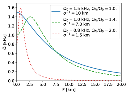
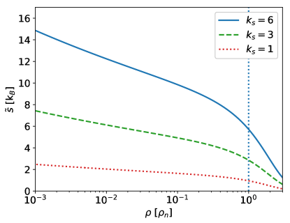
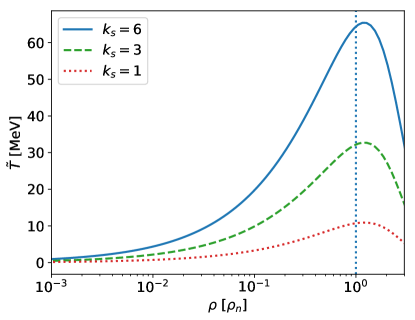
Figure 1: Dependence on the parameters of the rotation and thermal laws. $\tilde{\Omega}=-G^{\prime}(F)$ (top) is minus the derivative of the rotation law and $\tilde{s}$ (center) and $\tilde{T}$ (bottom) are two equivalent versions of the thermal law. If the star is effectively barotropic ($b=0$), then $\Omega=\tilde{\Omega},s=\tilde{s},T=\tilde{T}$. The vertical blue dotted line marks the saturation density.

III Results

III.1 Search

For each EOS, we run about 100,000 simulations in order to explore the parameter space, varying the following six parameters with a uniform distribution:

• central density $\rho_{0}=[2;10]\,\rho_{n}$.

• axial angular velocity $\Omega_{0}=[0;3]$ kHz.

• entropy scale $k_{s}=[1;9]$.

• maximal-to-axial angular velocity ratio $\Omega_{M}/\Omega_{0}=[1;2]$.

• rotation law scale $\sigma^{-1}=[1.5,10]$ km (we report it in km because it can be interpreted, approximately, as the radial scale of the rotation distribution at large distance from the rotation axis).

• baroclinic constant $b=[-2;0]$.

As already discussed, see Sec. II.2, the other parameters are set as follows: $G_{0}=0$, $F_{0}$ from Eq. (9), $\rho_{M}=\rho_{L}=\rho_{n}$, and $\Gamma_{T}=2/3$. The values and ranges of the parameters are chosen to approximately reproduce the models evolved by Hanauske et al. (2017) and Perego et al. (2019) (see Sec. III.4 for a comparison). In particular, we set $b<0$ so that there is a hot ring in the equatorial plane instead of two hot caps in the polar regions and its range is set to resemble the models of Perego et al. (2019) and Kastaun et al. (2016), and to include the effectively barotropic model as special case ($b\to 0$). The numerical details of how we find our solutions with a modified version of the XNS code are reported in Appendix A.2.

We remark that time evolution of the BNS remnant can be mimicked by varying the free input parameters of our model, once the remnant becomes stationary after a $\sim 10\,\mathrm{ms}$ timescale. In fact, shortly after merger, $b\to 0$ on a $t\simeq 50\,\mathrm{ms}$ timescale (Perego et al., 2019) and at later times, if the remnant does not collapse to a black hole, $k_{s}\to 0$ on a $t\simeq 10\,\mathrm{s}$ timescale due to the loss of entropy caused by neutrino emission. On this timescale the central density $\rho_{0}$ increases due to cooling and $\Omega_{M}/\Omega_{0}\to 1$ and $\sigma\to 0$ as the star approaches rigid rotation due to neutrino diffusion and magnetic viscosity (both of which we do not include). Whether the axial angular velocity $\Omega_{0}$ increases or decreases on a longer timescale depends on the total angular momentum loss by neutrino emission and magnetic braking (Ravi and Lasky, 2014; Lasky et al., 2014), on that gained by accretion, and by the evolution of the stellar moment of inertia. However, it is plausible to assume that the BNS merger remnant spins up as it happens for a proto-neutron star (Camelio et al., 2016).

Before discussing the results, we remark that only $\sim$ 7–8$\%$ of the parameter combinations in the searches gives a valid solution of the Einstein and Euler equations. The failure of a particular parameter combination may be due to the physics (e.g., the mass shedding limit has been exceeded) or to numerical issues (i.e., the code is not stable enough; a “false negative”). We increased the stability of the code by choosing physically motivated parameters and by slowly increasing the rotational and thermal content of the star at the beginning of the iterative process (see Appendix A.2). However, it is unavoidable that a fraction of the unsuccessful runs might consist of false negatives. On the other hand, the successful configuration are physical in the sense that they are solutions of the Einstein and Euler equations, but despite our efforts of realistic modeling we cannot be sure that they all approximate the result of dynamical evolution of mergers. For example, a small number of successful parameter combinations (of the order 10) results in stellar models with gravitational mass $M>4$. Considering BNS population scenarios, such high masses are astrophysically unlikely (but not impossible for rapidly rotating models with extremely stiff EOSs (Haskell et al., 2018)) for BNS merger remnants and we will exclude these configurations from the following analysis.

Unless otherwise stated, we will consider the ALF2 EOS in this section. The reason is that we can reliably invert the EOS and obtain the rest mass density $\rho$ and entropy per baryon $s$ from the pressure $p$ and the enthalpy density $\mathcalligra{h}\,\,$ only for this EOS (see Appendix A.1 for details). We checked that the other quantities follow the same qualitative trends of the ALF2 EOS, see for example Fig. 3.

The parameters and stellar quantities of the successful configurations found in the search can be downloaded from Zenodo (Camelio et al., 2020).

III.2 Stellar properties

By exploring several thousand configurations, we find that some combinations of the model parameters are either unphysical or not reproducible with our code, see Fig. 2 and discussion in Sec. III.1. In some cases, there is a reasonable physical motivation for trends observed in Fig. 2: for example, the maximum of the axial angular velocity $\Omega_{0}$ increases with density $\rho_{0}$ (Fig. 2a), since gravity is stronger and it is possible to reach faster rotation without mass shedding, cf. Fig. 4b. Similarly, the maximum of the entropy scale $k_{s}$ increases with increasing density $\rho_{0}$ (Fig. 2b; the other EOSs reach $k_{s}=9$ with a similar trend of ALF2) and the maximum of the axial angular velocity $\Omega_{0}$ is greater for smaller rotation ratio $\Omega_{M}/\Omega_{0}$ (Fig. 2c), due to the necessity for the equatorial angular velocity to be lower than the Keplerian frequency in order to avoid mass shedding. On the other hand, the fact that the maximum of the rotation scale $\sigma^{-1}$ is greater for smaller rotation ratio $\Omega_{M}/\Omega_{0}$ is probably a spurious effect due to numerical issues, since in simulations Hanauske et al. (2017) the distance of the maximum of the angular velocity profile is at larger distances from the rotational axis than what we obtain with our code, see Figs. 2d and 8 and discussion in Sec. III.4. Remarkably, the position of the maximum of the angular velocity $F_{0}$ (which also serves as a scale for the inner part of the rotation law) is correlated with the baroclinic constant $b$, while it is not correlated with the central density $\rho_{0}$ (Figs. 2e-f) and with $k_{s}$.

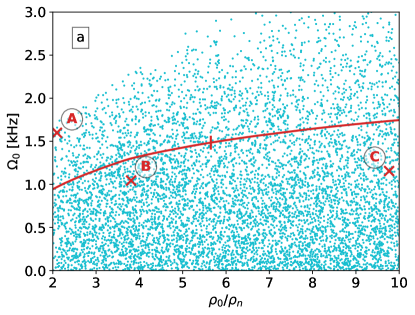
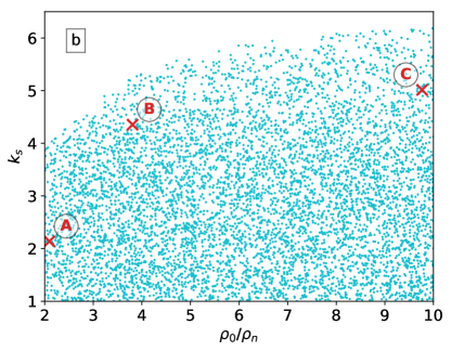
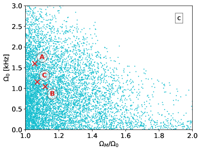
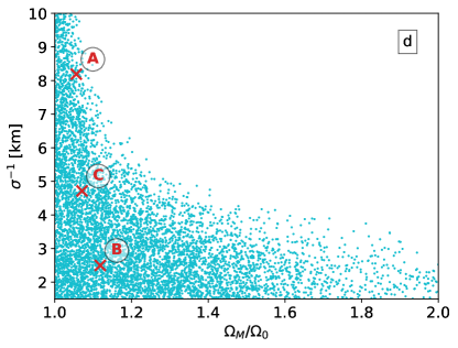
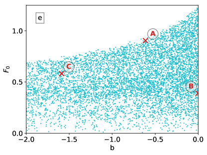
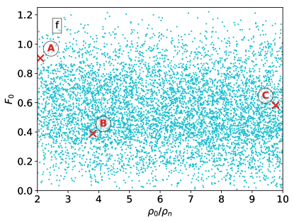
Figure 2: Parameter space of the BNS merger remnant with the ALF2 EOS. The blue dots are the successful runs with $M<4$ and the red line is the rigidly rotating, cold Keplerian curve, on which we marked the marginally stable configuration. We marked with red crosses the model described in Sec. III.4. $\rho_{0}$ is the central density, $\Omega_{0}$ the angular velocity on the rotational axis, $k_{s}$ the entropy scale, $\Omega_{M}/\Omega_{0}$ the ratio between the maximum and axial angular velocity in the rotation law, $\sigma^{-1}$ the rotation law scale, $F_{0}$ the critical point of the rotation law, and $b$ the baroclinic parameter.

For a given central density, the gravitational mass $M$ of our BNS merger remnant model is larger than the nonrotating mass and can even be larger than the cold rigidly rotating Keplerian one, see Fig. 3. In Fig. 4 we show some trends of other stellar quantities. These trends are obvious and expected: the stellar angular momentum $J$ grows with the axial angular velocity $\Omega_{0}$ (Fig. 4a), the maximum of the Keplerian angular velocity $\Omega_{\mathrm{kep}}$ grows with the central density $\rho_{0}$, and the average entropy per baryon $S/M_{0}$ grows with the entropy scale $k_{s}$. The circumferential radius $R_{\mathrm{cir}}$ grows with entropy scale $k_{s}$ (due to an increasing thermal pressure, Fig. 4e) and when the equatorial angular velocity $\Omega_{\mathrm{eq}}$ approaches the Keplerian one $\Omega_{\mathrm{kep}}$ (since the configuration approach mass shedding, Fig. 4f). Assuming that the configuration collapses to a black hole, one can estimate the mass of the accretion disk that remains outside of the innermost stable circular orbit (see discussion in Sec. III.4). The disk mass $M_{\mathrm{disk}}$ also grows when the equatorial angular velocity approaches the Keplerian one, as expected. It is worth pointing out that, when present, the estimated mass of the accretion disk is of the order of that expected from simulations, e.g., Refs. (Hanauske et al., 2017; Radice et al., 2018; Coughlin et al., 2019; Dietrich et al., 2020), and much larger than the one that is expected from a single rotating NS (Margalit et al., 2015; Camelio et al., 2018).

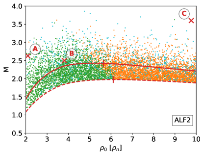
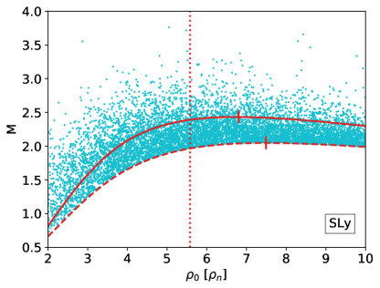
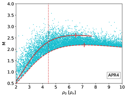
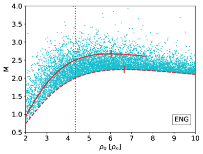
Figure 3: Mass $M$ vs. central density $\rho_{0}$ for each EOS. Plotting conventions as in Fig. 2; in addition the red dashed line is the nonrotating curve on which we marked the maximal mass configuration and the vertical dotted line is the critical density $\rho_{c}$ for the EOS inversion, see Appendix A.1. For the ALF2 EOS, we colored each point according to criterion (16): green and orange points are expected to be stable and unstable, respectively, while we do not known the value of Eq. (16) for blue points (due to numerical issues). We stress that this stability criterion [Eq. (16)] cannot be applied to our model and we report it here only as an indication, see discussion in Sec. III.3 for details.

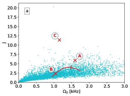
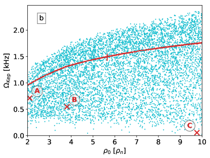
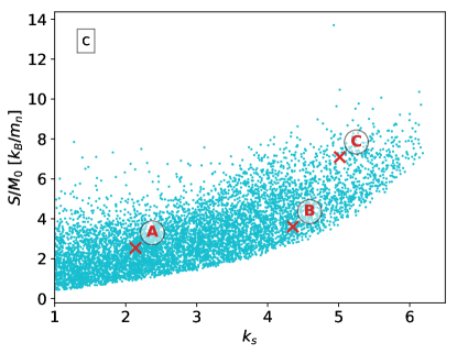
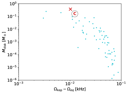
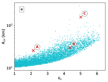
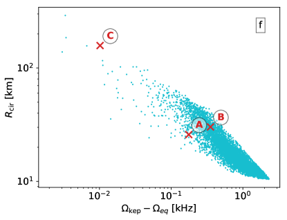
Figure 4: Stellar properties of the BNS merger remnant with the ALF2 EOS. Plotting conventions as in Fig. 2. $\Omega_{0}$ is the angular velocity on the rotational axis, $J$ the angular momentum, $\rho_{0}$ the central density, $\Omega_{\mathrm{kep}}$ the Keplerian angular velocity at the equator, $k_{s}$ the entropy scale parameter, $S/M_{0}$ the average (per baryon mass) stellar entropy, $\Omega_{\mathrm{eq}}$ the angular velocity at the equator, $M_{\mathrm{disk}}$ the expected baryon mass of the accretion disk, and $R_{\mathrm{cir}}$ the circumferential equatorial radius.

III.3 Stability

The solutions that are found for a given EOS are not necessarily dynamically stable. There are many types of instabilities that may be present (for a review see e.g. Friedman and Stergioulas, 2011), and whether or not a particular one is relevant depends on how its associated timescale compares with the timescale of the viscous processes at work. In this paper, we will consider a non-comprehensive set of possible instabilities that may be present in the remnant.

Low $\mathcal{T}/|W|$-instability: The dynamical study of differentially rotating configurations allowed the discovery of the so-called “low-$\mathcal{T}/|W|$ instability” (Centrella et al., 2001; Watts et al., 2005; Passamonti and Andersson, 2020). The low-$\mathcal{T}/|W|$ instability sets in when an oscillation mode co-rotates with the matter in a point of the star. Since in a BNS merger remnant the angular velocity is not monotonic with the radius, it is possible for an oscillation mode to co-rotate with the matter in two points (Passamonti and Andersson, 2020; Xie et al., 2020). Performing the numerical evolution in General Relativity of an initially cold remnant with a rotation law from Uryū et al. (2017), Xie et al. (2020) found that this instability is present for the relatively low value of $\mathcal{T}/|W|=0.16$, where $\mathcal{T}$ is the kinetic energy (not to be confused with the temperature) and $W=M_{p}+\mathcal{T}-M$ is the gravitational binding energy ($M_{p}$ is the proper mass). Similarly, making use of Newtonian gravity, assuming the Cowling approximation, and exploring a larger number of remnant configurations, Passamonti and Andersson (2020) found that this instability may set in for $\mathcal{T}/|W|\gtrsim 0.02$ and as $\mathcal{T}/|W|$ grows it initially becomes more relevant until the mode stabilizes to a specific value of $\mathcal{T}/|W|$. We find that $\mathcal{T}/|W|$ grows for increasing axial angular velocity $\Omega_{0}$ (Fig. 5a), and that the maximum of $\mathcal{T}/|W|$ decreases with increasing entropy scale $k_{s}$ (Fig. 5b) and increasing rotational scale $\sigma^{-1}$ (Fig. 5c). The anti-correlation between $\mathcal{T}/|W|$ and $k_{s}$ is not mediated through the central density $\rho_{0}$ since both $\Omega_{0}$ and $k_{s}$ increase with increasing $\rho_{0}$, cf. Figs. 2a-b. We interpret the anti-correlation of $k_{s}$ and $\mathcal{T}/|W|$ with the fact that, increasing the thermal pressure, the star is less strongly bound. We conclude that a larger entropy content contributes in stabilizing the star against the low-$\mathcal{T}/|W|$ instability.

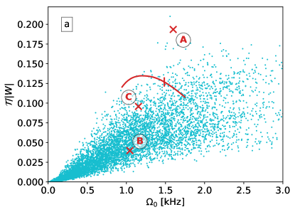
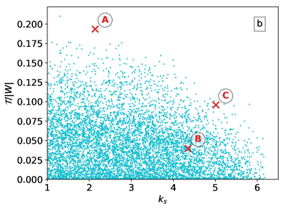
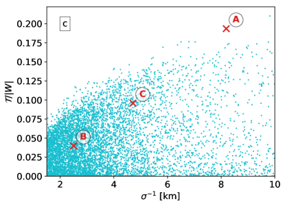
Figure 5: Kinetic-to-gravitational binding energy ratio $\mathcal{T}/|W|$ of the BNS merger remnant with the ALF2 EOS. Plot conventions as in Fig. 2. $\Omega_{0}$ is the angular velocity on the rotational axis, $k_{s}$ the entropy scale parameter, and $\sigma^{-1}$ the rotation law scale.

Convective instability: The convective instability has a local character and sets in when a displaced fluid element is accelerated away from its equilibrium position. In a hot, rotating star, the forces that are applied on a fluid element are gravity, buoyancy (due to the pressure gradient), and the centrifugal force (see e.g. Abramowicz, 2004).

In a non-rotating and hence spherical star, convective instability is driven by buoyancy. In this case, necessary conditions for convective instability are a non-barotropic EOS and entropy (or composition) gradients. For non-rotating NSs, the onset of convective instability is controlled by the Schwarzschild criterion (Thorne, 1966), that is, a star is convectively unstable when the Schwarzschild discriminant $\bar{S}(\bar{r})$ is negative,

$$\bar{S}(\bar{r})=\frac{\mathrm{d}p}{\mathrm{d}\bar{r}}-c_{s}^{2}\frac{\mathrm{d}\epsilon}{\mathrm{d}\bar{r}}<0,$$ (12)

where $\bar{r}$ is the Schwarzschild radius and $c_{s}^{2}$ the speed of sound. As pointed out in Camelio et al. (2019), for our EOS this is identical to

$$\Big{[}(\Gamma_{\mathrm{th}}-1)(1+a_{i})\rho+\Gamma_{i}k_{i}(\Gamma_{\mathrm{th}}-\Gamma_{i})\rho^{\Gamma_{i}}\Big{]}\frac{\mathrm{d}s}{\mathrm{d}\bar{r}}<0,$$ (13)

or, equivalently (since in our case $\Gamma_{\mathrm{th}}<\Gamma_{i}$), a star is unstable against convection if

$$\operatorname{sgn}(\rho_{c}-\rho)\cdot\operatorname{sgn}\left(\frac{\mathrm{d}s}{\mathrm{d}\bar{r}}\right)<0,$$ (14)

where the critical density $\rho_{c}$ happens to be the same critical density for the EOS inversion (see Appendix A.1; the value of $\rho_{c}$ for each EOS is reported in Table 2 and marked with a vertical line in Fig. 3). In our case, since the thermal law for the effective barotropic case is such that $\mathrm{d}s/\mathrm{d}\rho>0$ [we set $\Gamma_{T}=2/3$ in Eq. (10)], Eq. (14) tells us that if the density decreases monotonically from the center outward, then the star is stable in the region with $\rho<\rho_{c}$ and unstable for $\rho>\rho_{c}$.

On the other hand, in isentropic stars the driver for convective instability is the centrifugal force. When the isentropic star is differentially rotating, a necessary criterion for convective stability is (Bardeen, 1970; Friedman and Stergioulas, 2011)

$$\frac{\mathrm{d}j^{2}(r,\pi/2)}{\mathrm{d}r}>0,$$ (15)

where the square of the specific (per unit mass) angular momentum $j=\mathcalligra{h}\,\,u_{\phi}/\rho$ is differentiated along the equatorial plane, $\theta=\pi/2$. As shown in the top panel of Fig. 7, this criterion is generally respected with our differential rotation law.

Having a configuration that is differentially rotating, non-isentropic, and baroclinic (namely non effectively barotropic) at the same time means that the simple criteria (12) and (15) are no more valid. This is due to the fact that not only the gravitational force is no more balanced by the buoyant force alone, but also to the fact that the three forces are not necessary parallel. However, due to the qualitative nature of our discussion, we will still make use of criteria (14) and (15) to allow for this simple remark on the remnant stability: that an increase of $\rho_{0}$ favors a buoyancy-driven convective instability, because configurations with $\rho_{0}>\rho_{c}$ (right of the dotted line in Fig. 3) are convectively unstable (at least in a part of the star), while configurations $\rho_{0}<\rho_{c}$ (left of the dotted line in Fig. 3) are convectively stable if the density decreases monotonically with the radius everywhere (and the entropy increases with the radius). Note that convective instability has been found 30-50 ms after merge in numerical simulations (De Pietri et al., 2018, 2020), and some of our models do have negative entropy gradients at intermediate radii. We remark moreover that this already approximate consideration is valid only for the simplified EOSs we are considering. In a more realistic EOS, the value of $\Gamma_{\mathrm{th}}$ may be density-dependent and the simple non-rotating convective instability criterion we derived, see Eqs. (13)–(14), should be revised.

Axisymmetric secular stability: Another type of instability is the “secular instability”. It sets in when a configuration evolves to a similar one with lower energy (i.e. a stabler one) on a timescale longer than the hydrodynamical one. Here we are concerned with axisymmetric instabilities, which can be determined simply by studying the stationary (axisymmetric) configurations. In practice, a configuration defined by a set of parameters is stable if all configurations close in the parameter space with the same baryon mass $M_{0}$, angular momentum $J$, and total entropy $S$, have a greater gravitational mass $M$. For rigidly rotating, isentropic NSs, secular stability can be checked with the turning point criterion (Sorkin, 1981, 1982; Friedman et al., 1988; Goussard et al., 1997), that is, a star becomes secularly unstable when

$$\left.\frac{\partial M}{\partial\rho_{0}}\right|_{J,S}=0,$$ (16)

where $\rho_{0}$ is the central density. In the case of a cold and non-rotating NS, secular instability implies and is implied by instability against dynamical perturbations (Misner and Zapolsky, 1964), while in general, for a rigidly rotating and isentropic star, secular instability is a sufficient but not necessary condition for instability against dynamical perturbations (e.g., Takami et al., 2011).

In the general case we are interested in, namely differentially rotating, non-isentropic, and baroclinic NSs, the turning point criterion [Eq. (16)] cannot be applied because the number of free parameters is greater than the number of conserved quantities (i.e., $M_{0},S,J$ (Sorkin, 1982)). As an exercise, we applied anyway criterion (16) for the ALF2 EOS (for which we can compute $J$ and $S$) and showed the result in Fig. 3. We stress that this should be taken as an indication for stability, since we know that the turning point criterion cannot be applied to our case (see also footnote 6). In any case, we can draw a couple of simple conclusions from this exercise: (i) we cannot draw a clear stable/unstable line in the $\rho_{0}$-$M$ diagram, since it is a 2-dimensional projection of the 6-dimensional parameter space, and (ii) the marginally stable, cold, nonrotating and the cold, rigidly rotating, Keplerian configurations are in the region of the $\rho_{0}$-$M$ diagram where the transition from stability to instability for our model is expected.

Apart for the turning point criterion criterion, one can try to determine the stability of a configuration directly from the definition (namely that $M$ is a minimum for constant $M_{0},J,S$). A problem of this approach is that two configurations close in the parameter space may not be connected by any dynamical evolution, and therefore it would not make sense to compare their gravitational mass. In the case of the ALF2 EOS, for which we can compute $M_{0}$ and $S$, we tried anyway to look at the variation of $M$ with respect to the parameters, keeping $M_{0},J,S$ constant. Unfortunately, we were not able to draw clear conclusions from this analysis and further work is required.

III.4 Selected models

In this section we show the stellar profiles for three selected models, chosen according to the following criteria:

• A model that is a plausible outcome of a BNS merger.

• The model with $M<4$ that is closest to an effectively barotropic configuration, namely that with the baroclinic parameter $b$ closest to zero, to be compared with model A.

• The model with the greatest disk mass and $M<4$.

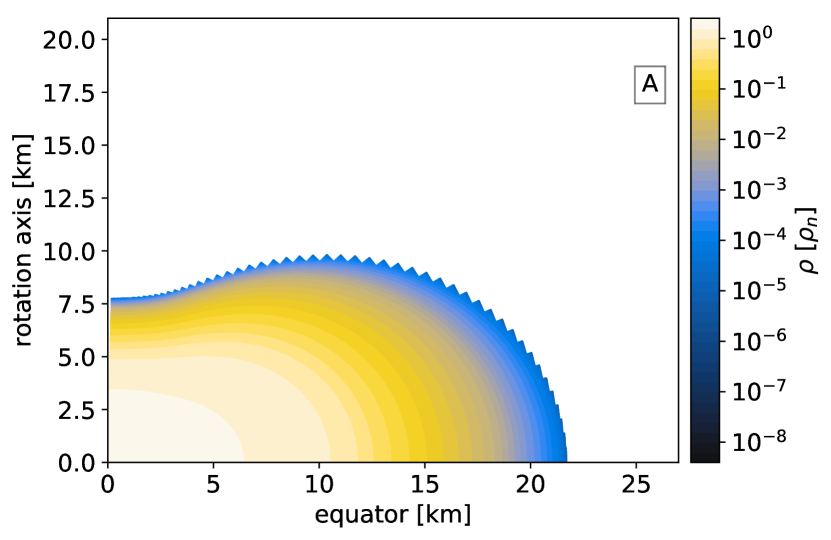
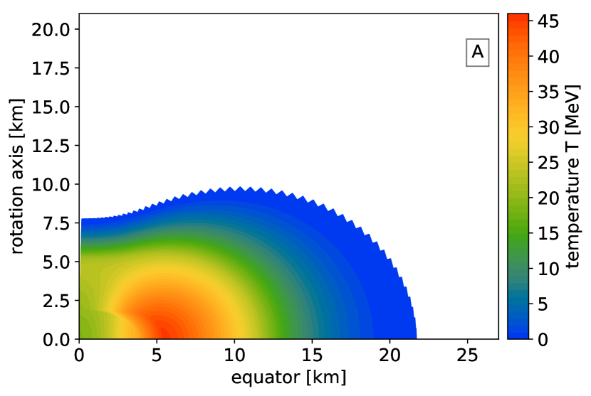
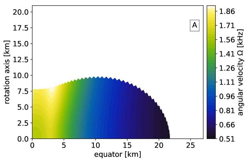
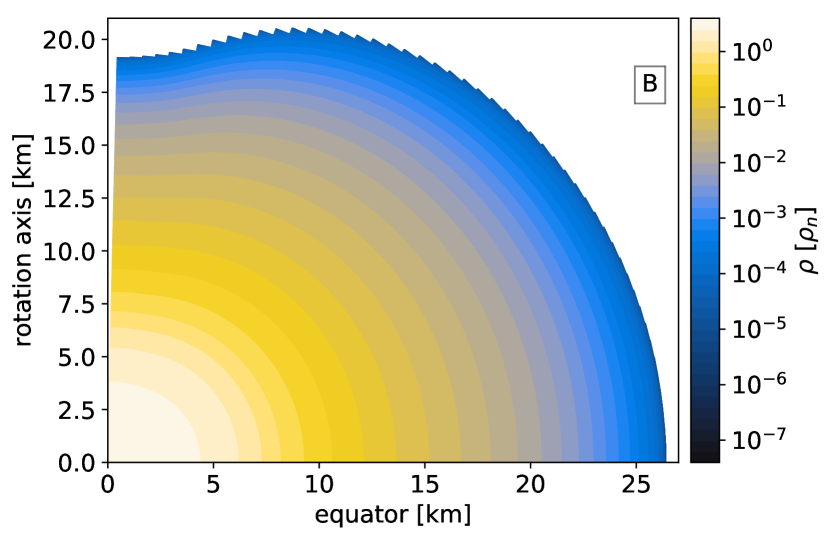
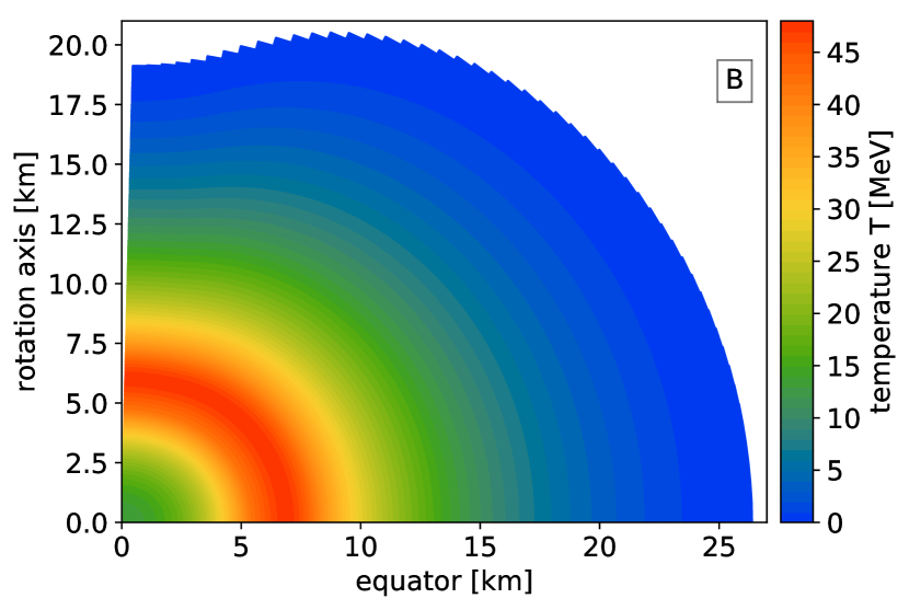
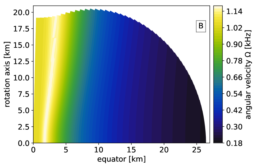
Figure 6: Density $\rho$, temperature $T$, and angular velocity $\Omega$ profiles of models A and B.

The specific model parameters and properties are summarized in Table 1 and their rest mass density, temperature, and angular velocity distribution are shown in Figs. 6–9.

Model A is a realistic BNS merger remnant. Its mass $M$, angular momentum $J$, and central density $\rho_{0}$ are in the expected range, e.g., Tauris et al. (2017); Abbott et al. (2020). Its shape is qualitatively similar to that obtained in simulations, (cf. Fig. 13 in Perego et al. (2019)). The temperature forms a hot ring in the equatorial plane (cf. Fig. 7 of Perego et al. (2019)); the temperature profile is continuous but not smooth due to the fact that the EOS is piecewise defined. The angular velocity curve peaks 3–4 km from the rotational axis (cf. Fig. 5 of Hanauske et al. (2017), where the peak is expected at 7–10 km).

Baroclinicity is fundamental in order to obtain the right thermal distribution. This can be realized comparing the profiles of models A and B (the latter being almost effectively barotropic): in model A the density and temperature isocontours are not parallel and this permits the existence of the hot equatorial ring, while in model B they are parallel and as a consequence the temperature profile has an onion-like shape. This is a consequence of baroclinicity (Camelio et al., 2019).

Between the three chosen models, model C has the biggest circumferential radius and its equatorial angular velocity is the closest to the Keplerian one. Unsurprisingly, a significant amount of matter with large specific angular momentum is present. In case of black hole formation, this matter could form a disk. We followed the approach of Margalit et al. (2015) (see also Shapiro (2004) and Camelio et al. (2018)), namely we computed the baryon mass of the matter whose angular momentum per unit mass $j$ is larger than that of the innermost stable circular orbit of a black hole with the same mass and angular momentum of the original system. This is equivalent to assume that there is no angular momentum transfer or loss during the collapse and that dynamical effects like shocks play no role, which is clearly not true (e.g., Ravi and Lasky, 2014; Lasky et al., 2014), but at the same time it is a first order approximation that allows us to make a semi-quantitative estimations of the expected disk mass $M_{\mathrm{disk}}$. We found it to be $M_{\mathrm{disk}}\approx 0.4\,\mathrm{M_{\odot}}$, which is substantially larger than that expected from the collapse of a marginally stable, Keplerian, rigidly rotating, cold NS (Margalit et al., 2015; Camelio et al., 2018). The disk mass is in the range of what is expected from dynamical simulations (actually at the upper end of the expectations) (Hanauske et al., 2017; Radice et al., 2018; Coughlin et al., 2019; Dietrich et al., 2020; Bernuzzi, 2020; Nedora et al., 2020, 2021). With a large potential energy reservoir of $3.6\times 10^{52}\;{\rm erg}\;(\epsilon/0.05)(M_{\rm disk}/0.4M_{\odot})$, this configuration is a good candidate for launching a powerful short GRB, provided that the energy can be deposited in a low enough density environment. For the latter, one usually assumes that the central object needs to collapse to a black hole, but see Mösta et al. (2020) for the possibility to launch relativistic outflows in the presence of a central neutron star.

In Fig. 8 we compare the profiles of $\Omega(r)$ along the equator for our models A, B, and C and that obtained by Hanauske et al. (2017) from the merger of two $M=1.25$ stars with the ALF2 EOS and a $\Gamma_{\mathrm{th}}=1.8$ thermal component (Hanauske et al. (2017) found that the rotational profile of the remnant is almost independent from the value of $\Gamma_{\mathrm{th}}$, see their Fig. 16). Our model reproduces the qualitative features of the simulated rotational profiles (e.g., the off-axis maximum of the angular velocity), but there are quantitative differences. In particular, the maximum of the angular velocity is much closer to the rotational axis in our models rather than in Hanauske et al. (2017).

In Fig. 9 we show a histogram of the thermodynamical properties of the matter for model B and model C, alike those in Perego et al. (2019). First, we note the defining difference between the (almost) effectively barotropic configuration of model B and the baroclinic (i.e., nonbarotropic) configuration of model C: given a value of the density, there is only one value of temperature that can be obtained in model B, while this is not true for model C. Second, we remark that the models reproduce the qualitative features of the histograms in Perego et al. (2019) (e.g., the polytropic increase of the temperature with the density, the maximum of the temperature reached off-center, and the baroclinicity), but there are quantitative differences, most notably a smaller variation of the temperature for a given density in model C compared to the simulation results of Perego et al. (2019).

In future works, we will refine our model and the code in order to improve the quantitative comparison with the results of dynamical simulations.

We provide the community with 10 realistic BNS remnant models (including model A) with the ALF2 EOS and stellar properties in the ranges $2.4<M<3.5$, $5.5<J<7.5$, $1.5<\rho_{0}/\rho_{n}<4$, $\Omega_{M}/\Omega_{0}>1.05$, compatible to numerical relativity simulations, e.g., Dietrich et al. (2018); Kiuchi et al. (2020), plus models B and C. The stellar profiles and a python script to read them can be downloaded from Zenodo (Camelio et al., 2020). This dataset can be used as background models for microphysical studies or as initial conditions for dynamical evolution.

Table 1: Parameters and stellar quantities of the models shown in Sec. III.4. The EOS is ALF2. The quantities are: central density $\rho_{0}$, axial angular velocity $\Omega_{0}$, entropy scale $k_{s}$, angular velocity ratio $\Omega_{M}/\Omega_{0}$ and rotation law scale $\sigma^{-1}$, baroclinic parameter $b$, gravitational and baryon mass $M$ and $M_{0}$, stellar angular momentum $J$, average entropy per baryon mass $S/M_{0}$, kinetic-to-gravitational energy ratio $\mathcal{T}/|W|$, circumferential radius $R_{\mathrm{cir}}$, Keplerian angular velocity at the equator $\Omega_{\mathrm{kep}}$, angular velocity at the equator $\Omega_{\mathrm{eq}}$, expected disk mass $M_{\mathrm{disk}}$, maximum temperature $T_{\mathrm{max}}$.

quantity	A	B	C
$\rho_{0}$ [$\rho_{n}$]	2.097	3.808	9.767
$\Omega_{0}$ [kHz]	1.599	1.044	1.154
$k_{s}$	2.138	4.354	5.015
$\Omega_{M}/\Omega_{0}$	1.056	1.118	1.071
$\sigma^{-1}$ [km]	8.189	2.497	4.714
$b$	$-0.6136$	$-2.465\times 10^{-4}$	$-1.589$
$M$ [$M_{\odot}$]	2.63	2.50	3.60
$M_{0}$ [$M_{\odot}$]	2.86	2.76	3.84
$J$ [$M_{\odot}^{2}$]	5.92	2.34	11.4
$S/M_{0}$ [$k_{B}/m_{n}$]	2.54	3.60	7.09
$\mathcal{T}/|W|$	0.194	0.0398	0.0958
$R_{\mathrm{cir}}$ [km]	25.9	30.2	158
$\Omega_{\mathrm{kep}}$ [kHz]	0.712	0.547	0.560
$\Omega_{\mathrm{eq}}$ [kHz]	0.536	0.193	0.458
$M_{\mathrm{disk}}$ [$M_{\odot}$]	0.00	0.00	0.372
$T_{\mathrm{max}}$ [MeV]	45.5	47.5	112

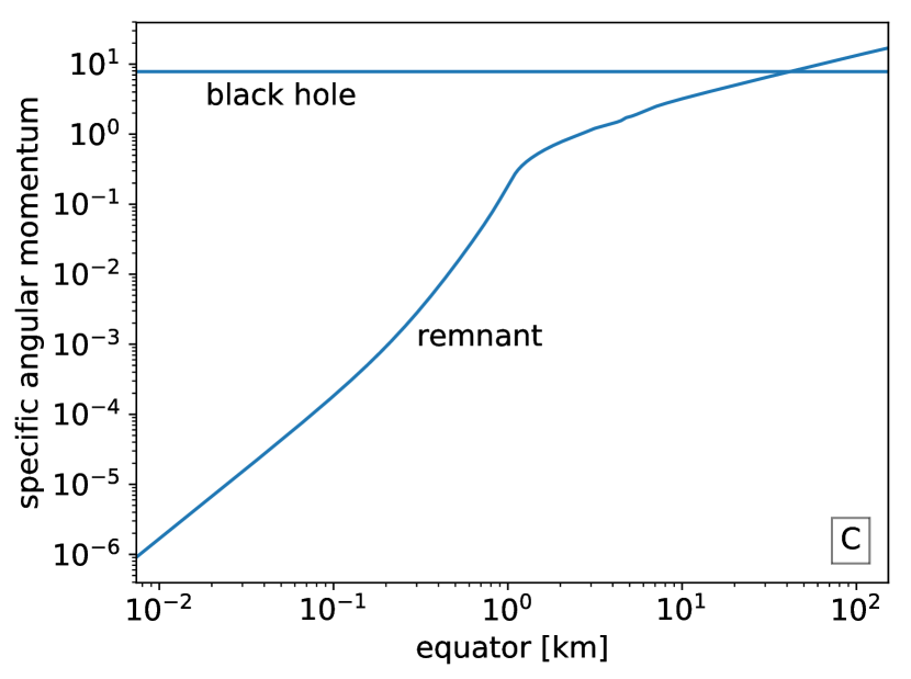
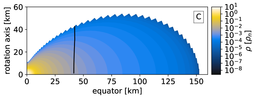
Figure 7: Angular momentum per unit mass along the equator ($j$, top) and density profile ($\rho$, bottom) of model C. In the top panel, the horizontal line is the angular momentum per unit mass of the innermost stable circular orbit of the black hole with the same mass and angular momentum of model C. In the bottom panel, the black line separates the matter expected to fall onto the black hole in case of stellar collapse from that forming the accretion disk.

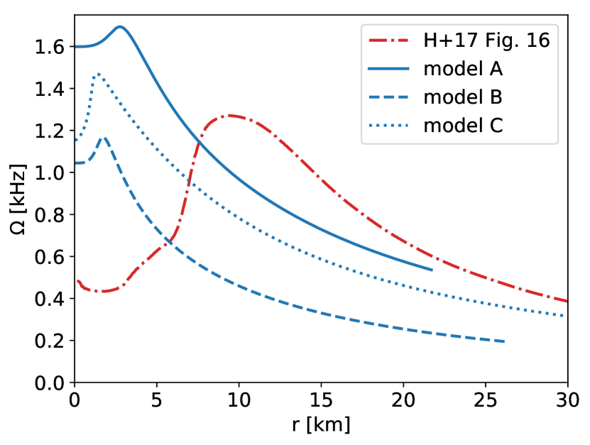
Figure 8: Rotational profiles of models A (straight blue line), B (dashed blue line), and C (dotted blue line) and of the ALF2-M125 $\Gamma_{\mathrm{th}}=1.8$ model of Hanauske et al. (Fig. 16 of Ref. 2017) (dot-dashed red line).

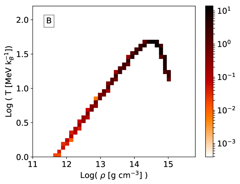
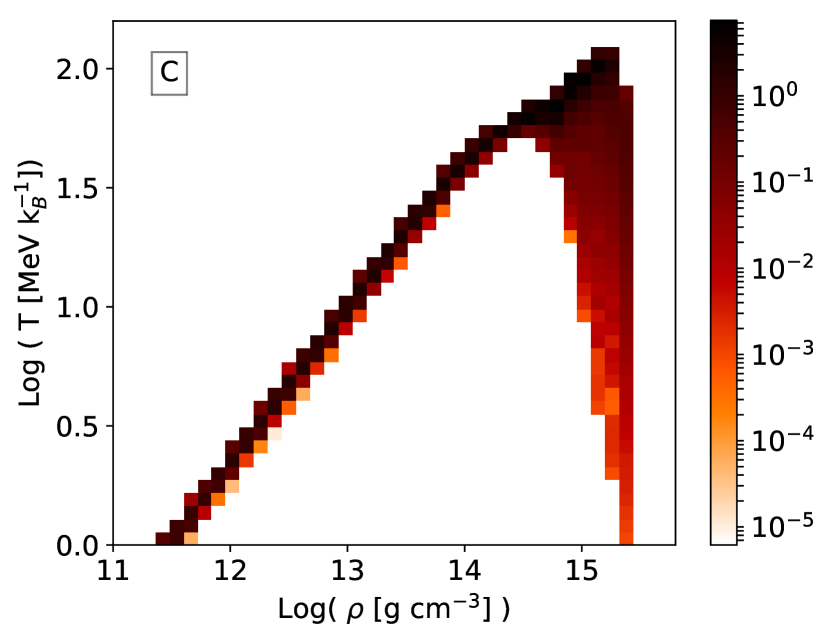
Figure 9: Mass-weighted, normalized histogram of the thermodynamical distribution (temperature vs rest mass density) of matter for models B (top) and C (bottom), to be compared with Perego et al. (2019).

IV Conclusion

In this paper we studied realistic stationary models for post-merger configurations after a BNS merger. We modeled the EOS with cold polytropic pieces (Read et al., 2009) plus a thermal component as described in more detail in (Camelio et al., 2019). Our remnant model is controlled by the central density and other parameters that fix the rotational and thermal distributions. We explored a broad range of post-merger configurations and discussed their stability based on qualitative criteria.

In particular we have

• introduced new rotation and thermal laws, Eqs. (8) and (10), that are motivated by numerical simulations (Hanauske et al., 2017; Perego et al., 2019).

• applied the technique recently developed by Camelio et al. (2019) to BNS merger remnants. We obtained baroclinic (i.e., not effectively barotropic) configurations, which are more suitable to model merger remnants than the effectively barotropic ones (Perego et al., 2019).

• performed an extensive parameter space study in which we included the effects of differential rotation, temperature, and baroclinicity.

Our main results are:

• the central density $\rho_{0}$, the axial angular velocity $\Omega_{0}$, and the thermal scale $k_{s}$ are the parameters that have the largest impact on the global remnant properties, see Fig. 4.

• baroclinicity (implemented with the parameter $b$) is necessary to reproduce the thermodynamical profile of BNS merger remnants, in particular the existence of a hot ring in the equatorial plane (Perego et al., 2019; Kastaun et al., 2016), compare models A and B in Sec. III.4.

• the collapse of a BNS merger remnant to a black hole may generate a massive disk which could provide the central engine to launch a short gamma ray burst (Margalit et al., 2015; Camelio et al., 2018), see Figs. 4d and 7.

• the increase of the central density $\rho_{0}$ may cause convective instabilities and the increase of the axial angular velocity $\Omega_{0}$ may cause low-$\mathcal{T}/|W|$ instability. If no convection is present, an increased thermal content ($k_{s}$) seems to increase stability by reducing the maximal $\mathcal{T}/|W|$ that can be reached by the model.

• we make the results of our parameter search and a set of realistic models available to the community (Camelio et al., 2020).

The approach described here can be extended further:

• an even more realistic description of the remnant physics, namely (i) the inclusion of composition in the model, (ii) the adoption of more realistic EOSs (for example the new piecewise parametrization of O’Boyle et al. (2020) or a tabulated EOS), (iii) the addition of the magnetic field (see Ref.  Lander et al., 2021, for an example of proto neutron star studied in Newtonian gravity), and (iv) the use of a rotation curve that is truly Keplerian by construction, not only because it approaches the Keplerian trend at large radii (like in this work and in Uryū et al. (2017)), but also the Keplerian frequency.

• addition of physically motivated restrictions on the free parameters of the stationary remnant model to simplify the study of its stability and the test of these predictions with dynamical simulations (Hanauske et al., 2017; Camelio et al., 2018) and/or a perturbative study (Krüger and Kokkotas, 2020a, b).

In this way it will be possible to perform realistic fits of the mergers remnant obtained by dynamical simulations.

Appendix A Implementation details

A.1 Equation of state

We adopt a set of EOSs obtained with different methods and different components: ALF2 (nuclear-quark hybrid EOS, Alford et al., 2005), SLy (nuclear EOS from an effective potential, Douchin and Haensel, 2001), APR4 (nuclear EOS from variational method, Akmal et al., 1998), and ENG (relativistic Brueckner-Hartree-Fock nuclear EOS, Engvik et al., 1996). We use the parametrization of Read et al. (2009) to implement them, including the SLy crust (we use only one index $i=1,\ldots,7$ running from the crust to high density). We summarize the EOS properties in Table 2.

In order to recover $\rho,s$ from $\mathcalligra{h}\,\,,p$, we note that Eq. (B14) of Camelio et al. (2019) can be generalized to

$$(\Gamma_{\mathrm{th}}-1)(1+a_{i})\rho+(\Gamma_{\mathrm{th}}-\Gamma_{i})k_{i}\rho^{\Gamma_{i}}\\ =(\Gamma_{\mathrm{th}}-1)\mathcalligra{h}\,\,-\Gamma_{\mathrm{th}}p.$$ (17)

Given a couple of $\mathcalligra{h}\,\,,p$ we can get 0, 1, or more different couples of $\rho,s$, see Fig. 10. It is important to know if the couple $\mathcalligra{h}\,\,,s$ admits at least one solution, because otherwise such couple is not valid and the algorithm should be able to mark that point as “vacuum outside the surface”. On the other hand, whether or not the solution of the EOS is unique is somehow less important because the only quantities that enter in the Einstein and Euler equations for an ideal gas are $\mathcalligra{h}\,\,$ and $p$ and not $\rho$ and $s$. This means that one can find a valid stellar configuration without knowing the rest mass and entropy distributions inside the star.

In the case of a piecewise polytropic EOS such as Eq. (1), the degeneracy can in principle be more problematic than for a 1-piece polytropic one because there can be more than 2 valid $\rho,s$ couples for given $\mathcalligra{h}\,\,,p$. An analysis of the piecewise EOSs considered in this paper shows that this is not the case: the degeneracy is the same of the one-piece polytropic EOS of Camelio et al. (2019), i.e., there is only one critical density $\rho_{c}$ in the range of the last high-density piece, $\rho_{c}>\rho_{6}$. In Table 2 we report the critical density for each EOS considered; apart for the ALF2 EOS, for which $\rho_{c}\simeq 45\rho_{n}$, the other critical densities lie in the range $4\rho_{n}\lesssim\rho_{c}\lesssim 6\rho_{n}$ and are even lower than the central density of the maximal mass configuration of the spherical (nonrotating) model. Since the ALF2 has such a high value of $\rho_{c}$, we can safely choose the low density branch of the solution like we did in Camelio et al. (2019), while we cannot do the same for the other EOSs. For this reason, we are able to compute the total stellar rest mass $M_{0}$, entropy $S$, and disk mass $M_{\mathrm{disk}}$ only for ALF2. All other quantities, such the stellar gravitational mass $M$ and angular momentum $J$, can be computed also for the other EOSs.

Table 2: EOS properties. For each EOS, we report: the EOS high-density polytropic index $\Gamma_{7}$; the EOS thermal constant $k_{\mathrm{th}}$; the temperature $T_{2,2}=T(2\rho_{n},2\,\mathrm{k_{B}})$; the critical density for the EOS inversion $\rho_{c}$; the central density $\rho_{\mathrm{tov}}$ of the maximal mass $M_{\mathrm{tov}}$ non-rotating configuration; the circumferential radius $R_{\mathrm{1.4}}$ of the non-rotating configuration with $M=1.4$; the maximum stellar angular momentum $J_{M}^{r}$, maximum angular rotation $\Omega_{M}^{r}$, and maximal mass $M_{M}^{r}$ on the stable branch of the Keplerian curve of a rigidly rotating and cold NS.

quantity	ALF2	SLy	APR4	ENG
$\Gamma_{7}$	1.890	2.851	3.348	3.168
$k_{\mathrm{th}}$	1.993	1.215	0.9610	1.385
$T_{2,2}$ [MeV]	37.9	23.1	18.3	26.3
$\rho_{\mathrm{c}}$ [$\rho_{n}$]	45.0	5.58	4.44	4.35
$\rho_{\mathrm{tov}}$ [$\rho_{n}$]	6.11	7.49	7.14	6.65
$M_{\mathrm{tov}}$ [$M_{\odot}$]	1.98	2.05	2.19	2.24
$R_{1.4}$ [km]	12.5	11.6	11.2	11.8
$J_{M}^{r}$ [$M_{\odot}^{2}$]	4.07	4.03	4.83	5.03
$\Omega_{M}^{r}$ [kHz]	1.48	1.85	1.98	1.85
$M_{M}^{r}$ [$M_{\odot}$]	2.43	2.43	2.61	2.68

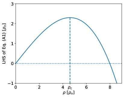
Figure 10: LHS of Eq. (17) for the $\Gamma=3$ EOS of Camelio et al. (2019). $\rho_{c}$ is the critical density for the inversion.

A.2 Neutron star

We used a modified version (Camelio et al., 2018, 2019) of the XNSv2 code (Bucciantini and Del Zanna, 2011; Pili et al., 2014); we refer the reader to the original papers for details on the implementation. The only difference with respect to our previous work (Camelio et al., 2019) is that, at the beginning of the iterative procedure to determine the stellar configuration, we have slowly increased the thermal and rotational content of the star by varying $k_{s}$ and $\Omega_{0}$, in order to increase the stability of the numerical scheme. We set the following parameters in our code:

• inner radial grid: boundary at $r=30\,\mathrm{M_{\odot}}$, $3000$ evenly spaced points,

• outer radial grid: boundary at $1000\,\mathrm{M_{\odot}}$, $3000$ increasingly spaced points,

• absolute tolerance of $\max(\mathcalligra{h}\,\,)$ for convergence: $10^{-11}$,

• planar symmetry,

• $50$ points in the angular grid (in one of the hemispheres),

• $500$ relaxing iterations (see discussion above),

• $30$ Legendre polynomials.

In order to implement the rotation law (8), we define two functions $G_{1}$ and $G_{2}$:

$$G_{1}(F)={} \bar{G}(F)\Theta(F_{0}-F)+G(F)\Theta(F-F_{0}),$$ (19)

$$G_{2}(F)={} G(F)\Theta(F_{0}-F)+\bar{G}(F)\Theta(F-F_{0}),$$ (20)

where $\Theta$ is the step function and

$$\bar{G}(F)=G_{0}-\frac{\Omega_{0}+\Omega_{M}}{2}F_{0}\\ -\Omega_{M}(F-F_{0})-(F-F_{0})^{3}.$$ (21)

We start by solving the system (3)–(4) with $G\equiv G_{1}$. If $F<F_{0}$, then we solve again the system with $G\equiv G_{2}$. We found that in this way we increase the precision of the solution close to the maximum, $F\simeq F_{0}$. Moreover, instead of solving the Newton-Raphson with $F$ as independent variable, we found that it is numerically more stable to solve the equations using $\Omega$ as independent variable, even if the rotation law is defined in $F$.

The heat function [Eq. (7)] is determined by numerical integration.

References

- Lattimer [2012] James M. Lattimer. The nuclear equation of state and neutron star masses. Ann. Rev. Nucl. Part. Sci., 62:485–515, 2012. doi: 10.1146/annurev-nucl-102711-095018.
- Benhar and Fantoni [2020] O. Benhar and S. Fantoni. Nuclear Matter Theory. CRC Press, Boca Raton, 2020.
- Abbott and al. [2017a] B. P. Abbott and al. GW170817: Observation of Gravitational Waves from a Binary Neutron Star Inspiral. Phys. Rev. Lett., 119(16):161101, October 2017a. doi: 10.1103/PhysRevLett.119.161101.
- Perego et al. [2019] Albino Perego, Sebastiano Bernuzzi, and David Radice. Thermodynamics conditions of matter in neutron star mergers. European Physical Journal A, 55(8):124, August 2019. doi: 10.1140/epja/i2019-12810-7.
- Hanauske et al. [2017] Matthias Hanauske, Kentaro Takami, Luke Bovard, Luciano Rezzolla, José A. Font, Filippo Galeazzi, and Horst Stöcker. Rotational properties of hypermassive neutron stars from binary mergers. Phys. Rev. D, 96(4):043004, August 2017. doi: 10.1103/PhysRevD.96.043004.
- Abbott and al. [2017b] B. P. Abbott and al. Multi-messenger Observations of a Binary Neutron Star Merger. ApJ, 848(2):L12, October 2017b. doi: 10.3847/2041-8213/aa91c9.
- Bauswein and Janka [2012] A. Bauswein and H.-Th. Janka. Measuring neutron-star properties via gravitational waves from binary mergers. Phys. Rev. Lett., 108:011101, 2012. doi: 10.1103/PhysRevLett.108.011101.
- Bauswein et al. [2014] A. Bauswein, N. Stergioulas, and H.-T. Janka. Revealing the high-density equation of state through binary neutron star mergers. Phys. Rev. D, 90(2):023002, 2014. doi: 10.1103/PhysRevD.90.023002.
- Takami et al. [2014] Kentaro Takami, Luciano Rezzolla, and Luca Baiotti. Constraining the Equation of State of Neutron Stars from Binary Mergers. Phys. Rev. Lett., 113(9):091104, 2014. doi: 10.1103/PhysRevLett.113.091104.
- Takami et al. [2015] Kentaro Takami, Luciano Rezzolla, and Luca Baiotti. Spectral properties of the post-merger gravitational-wave signal from binary neutron stars. Phys. Rev. D, 91(6):064001, 2015. doi: 10.1103/PhysRevD.91.064001.
- Bernuzzi et al. [2015] Sebastiano Bernuzzi, Tim Dietrich, and Alessandro Nagar. Modeling the complete gravitational wave spectrum of neutron star mergers. Phys. Rev. Lett., 115(9):091101, 2015. doi: 10.1103/PhysRevLett.115.091101.
- Bernuzzi [2020] Sebastiano Bernuzzi. Neutron star merger remnants. General Relativity and Gravitation, 52(11):108, November 2020. doi: 10.1007/s10714-020-02752-5.
- Wu et al. [2017] Meng-Ru Wu, Irene Tamborra, Oliver Just, and Hans-Thomas Janka. Imprints of neutrino-pair flavor conversions on nucleosynthesis in ejecta from neutron-star merger remnants. Phys. Rev. D, 96(12):123015, December 2017. doi: 10.1103/PhysRevD.96.123015.
- Abbar and Duan [2018] Sajad Abbar and Huaiyu Duan. Fast neutrino flavor conversion: Roles of dense matter and spectrum crossing. Phys. Rev. D, 98(4):043014, August 2018. doi: 10.1103/PhysRevD.98.043014.
- Tamborra and Shalgar [2020] Irene Tamborra and Shashank Shalgar. New Developments in Flavor Evolution of a Dense Neutrino Gas. arXiv e-prints, art. arXiv:2011.01948, November 2020.
- Hachisu [1986] I. Hachisu. A Versatile Method for Obtaining Structures of Rapidly Rotating Stars. ApJS, 61:479, July 1986. doi: 10.1086/191121.
- Komatsu et al. [1989] Hidemi Komatsu, Yoshiharu Eriguchi, and Izumi Hachisu. Rapidly rotating general relativistic stars. I - Numerical method and its application to uniformly rotating polytropes. MNRAS, 237:355–379, March 1989. doi: 10.1093/mnras/237.2.355.
- Uryū et al. [2017] Kōji Uryū, Antonios Tsokaros, Luca Baiotti, Filippo Galeazzi, Keisuke Taniguchi, and Shin’ichirou Yoshida. Modeling differential rotations of compact stars in equilibriums. Phys. Rev. D, 96(10):103011, November 2017. doi: 10.1103/PhysRevD.96.103011.
- Shibata et al. [2005] Masaru Shibata, Keisuke Taniguchi, and K ōji Uryū. Merger of binary neutron stars with realistic equations of state in full general relativity. Phys. Rev. D, 71:084021, Apr 2005. doi: 10.1103/PhysRevD.71.084021. URL https://link.aps.org/doi/10.1103/PhysRevD.71.084021.
- Kastaun and Galeazzi [2015] Wolfgang Kastaun and Filippo Galeazzi. Properties of hypermassive neutron stars formed in mergers of spinning binaries. Phys. Rev. D, 91:064027, Mar 2015. doi: 10.1103/PhysRevD.91.064027. URL https://link.aps.org/doi/10.1103/PhysRevD.91.064027.
- Kastaun et al. [2016] W. Kastaun, R. Ciolfi, and B. Giacomazzo. Structure of stable binary neutron star merger remnants: A case study. Phys. Rev. D, 94:044060, Aug 2016. doi: 10.1103/PhysRevD.94.044060. URL https://link.aps.org/doi/10.1103/PhysRevD.94.044060.
- Passamonti and Andersson [2020] A. Passamonti and N. Andersson. Merger-inspired rotation laws and the low-T/W instability in neutron stars. MNRAS, 498(4):5904–5915, September 2020. doi: 10.1093/mnras/staa2725.
- Xie et al. [2020] Xiaoyi Xie, Ian Hawke, Andrea Passamonti, and Nils Andersson. Instabilities in neutron-star postmerger remnants. Phys. Rev. D, 102(4):044040, August 2020. doi: 10.1103/PhysRevD.102.044040.
- Iosif and Stergioulas [2021] Panagiotis Iosif and Nikolaos Stergioulas. Equilibrium sequences of differentially rotating stars with post-merger-like rotational profiles. Monthly Notices of the Royal Astronomical Society, 503(1):850–866, 02 2021. ISSN 0035-8711. doi: 10.1093/mnras/stab392. URL https://doi.org/10.1093/mnras/stab392.
- Goussard et al. [1997] J. O. Goussard, P. Haensel, and J. L. Zdunik. Rapid uniform rotation of protoneutron stars. A&A, 321:822–834, May 1997.
- Camelio et al. [2019] Giovanni Camelio, Tim Dietrich, Miguel Marques, and Stephan Rosswog. Rotating neutron stars with nonbarotropic thermal profile. Phys. Rev. D, 100(12):123001, December 2019. doi: 10.1103/PhysRevD.100.123001.
- Sorkin [1981] R. Sorkin. A Criterion for the Onset of Instability at a Turning Point. ApJ, 249:254, October 1981. doi: 10.1086/159282.
- Sorkin [1982] R. D. Sorkin. A Stability Criterion for Many Parameter Equilibrium Families. ApJ, 257:847, June 1982. doi: 10.1086/160034.
- Friedman et al. [1988] John L. Friedman, James R. Ipser, and Rafael D. Sorkin. Turning Point Method for Axisymmetric Stability of Rotating Relativistic Stars. ApJ, 325:722, February 1988. doi: 10.1086/166043.
- Takami et al. [2011] Kentaro Takami, Luciano Rezzolla, and Shin’ichirou Yoshida. A quasi-radial stability criterion for rotating relativistic stars. MNRAS, 416(1):L1–L5, September 2011. doi: 10.1111/j.1745-3933.2011.01085.x.
- Margalit et al. [2015] Ben Margalit, Brian D. Metzger, and Andrei M. Beloborodov. Does the Collapse of a Supramassive Neutron Star Leave a Debris Disk? Phys. Rev. Lett., 115(17):171101, October 2015. doi: 10.1103/PhysRevLett.115.171101.
- Camelio et al. [2018] Giovanni Camelio, Tim Dietrich, and Stephan Rosswog. Disc formation in the collapse of supramassive neutron stars. MNRAS, 480(4):5272–5285, November 2018. doi: 10.1093/mnras/sty2181.
- Ravi and Lasky [2014] Vikram Ravi and Paul D. Lasky. The birth of black holes: neutron star collapse times, gamma-ray bursts and fast radio bursts. MNRAS, 441(3):2433–2439, July 2014. doi: 10.1093/mnras/stu720.
- Lasky et al. [2014] Paul D. Lasky, Brynmor Haskell, Vikram Ravi, Eric J. Howell, and David M. Coward. Nuclear equation of state from observations of short gamma-ray burst remnants. Phys. Rev. D, 89(4):047302, February 2014. doi: 10.1103/PhysRevD.89.047302.
- Camelio et al. [2020] Giovanni Camelio, Tim Dietrich, Stephan Rosswog, and Brynmor Haskell. Axisymmetric models for neutron star merger remnants with realistic thermal and rotational profiles: dataset, 2020. URL https://zenodo.org/record/4268501.
- Read et al. [2009] Jocelyn S. Read, Benjamin D. Lackey, Benjamin J. Owen, and John L. Friedman. Constraints on a phenomenologically parametrized neutron-star equation of state. Phys. Rev. D, 79(12):124032, June 2009. doi: 10.1103/PhysRevD.79.124032.
- Bauswein et al. [2010] A. Bauswein, H. T. Janka, and R. Oechslin. Testing approximations of thermal effects in neutron star merger simulations. Phys. Rev. D, 82(8):084043, October 2010. doi: 10.1103/PhysRevD.82.084043.
- Yasin et al. [2018] Hannah Yasin, Sabrina Schäfer, Almudena Arcones, and Achim Schwenk. Equation of state effects in core-collapse supernovae. arXiv e-prints, art. arXiv:1812.02002, December 2018.
- Dietrich et al. [2020] Tim Dietrich, Michael W. Coughlin, Peter T. H. Pang, Mattia Bulla, Jack Heinzel, Lina Issa, Ingo Tews, and Sarah Antier. Multimessenger constraints on the neutron-star equation of state and the hubble constant. Science, 370(6523):1450–1453, 2020. ISSN 0036-8075. doi: 10.1126/science.abb4317. URL https://science.sciencemag.org/content/370/6523/1450.
- Alford et al. [2005] Mark Alford, Matt Braby, Mark Paris, and Sanjay Reddy. Hybrid Stars that Masquerade as Neutron Stars. ApJ, 629(2):969–978, August 2005. doi: 10.1086/430902.
- Douchin and Haensel [2001] F. Douchin and P. Haensel. A unified equation of state of dense matter and neutron star structure. A&A, 380:151–167, December 2001. doi: 10.1051/0004-6361:20011402.
- Akmal et al. [1998] A. Akmal, V. R. Pandharipande, and D. G. Ravenhall. Equation of state of nucleon matter and neutron star structure. Phys. Rev. C, 58(3):1804–1828, September 1998. doi: 10.1103/PhysRevC.58.1804.
- Engvik et al. [1996] L. Engvik, E. Osnes, M. Hjorth-Jensen, G. Bao, and E. Ostgaard. Asymmetric Nuclear Matter and Neutron Star Properties. ApJ, 469:794, October 1996. doi: 10.1086/177827.
- Bucciantini and Del Zanna [2011] N. Bucciantini and L. Del Zanna. General relativistic magnetohydrodynamics in axisymmetric dynamical spacetimes: the X-ECHO code. A&A, 528:A101, April 2011. doi: 10.1051/0004-6361/201015945.
- Pili et al. [2014] A. G. Pili, N. Bucciantini, and L. Del Zanna. Axisymmetric equilibrium models for magnetized neutron stars in General Relativity under the Conformally Flat Condition. MNRAS, 439(4):3541–3563, April 2014. doi: 10.1093/mnras/stu215.
- Isenberg [2008] James A. Isenberg. Waveless Approximation Theories of Gravity. International Journal of Modern Physics D, 17(2):265–273, January 2008. doi: 10.1142/S0218271808011997.
- Cordero-Carrión et al. [2009] Isabel Cordero-Carrión, Pablo Cerdá-Durán, Harald Dimmelmeier, José Luis Jaramillo, Jérôme Novak, and Eric Gourgoulhon. Improved constrained scheme for the Einstein equations: An approach to the uniqueness issue. Phys. Rev. D, 79(2):024017, January 2009. doi: 10.1103/PhysRevD.79.024017.
- Iosif and Stergioulas [2014] Panagiotis Iosif and Nikolaos Stergioulas. On the accuracy of the IWM-CFC approximation in differentially rotating relativistic stars. General Relativity and Gravitation, 46(10):1800, October 2014. doi: 10.1007/s10714-014-1800-5.
- Abramowicz [1971] M. A. Abramowicz. The Relativistic von Zeipel’s Theorem. Acta Astron., 21:81, January 1971.
- Camelio et al. [2016] Giovanni Camelio, Leonardo Gualtieri, José A. Pons, and Valeria Ferrari. Spin evolution of a proto-neutron star. Phys. Rev. D, 94(2):024008, July 2016. doi: 10.1103/PhysRevD.94.024008.
- Haskell et al. [2018] B. Haskell, J. L. Zdunik, M. Fortin, M. Bejger, R. Wijnands, and A. Patruno. Fundamental physics and the absence of sub-millisecond pulsars. A&A, 620:A69, December 2018. doi: 10.1051/0004-6361/201833521.
- Radice et al. [2018] David Radice, Albino Perego, Kenta Hotokezaka, Steven A. Fromm, Sebastiano Bernuzzi, and Luke F. Roberts. Binary Neutron Star Mergers: Mass Ejection, Electromagnetic Counterparts and Nucleosynthesis. Astrophys. J., 869(2):130, 2018. doi: 10.3847/1538-4357/aaf054.
- Coughlin et al. [2019] Michael W. Coughlin, Tim Dietrich, Ben Margalit, and Brian D. Metzger. Multimessenger Bayesian parameter inference of a binary neutron star merger. Mon. Not. Roy. Astron. Soc., 489(1):L91–L96, 2019. doi: 10.1093/mnrasl/slz133.
- Friedman and Stergioulas [2011] John L. Friedman and Nikolaos Stergioulas. Stability of relativistic stars. Bulletin of the Astronomical Society of India, 39:21–48, March 2011.
- Centrella et al. [2001] Joan M. Centrella, Kimberly C. B. New, Lisa L. Lowe, and J. David Brown. Dynamical Rotational Instability at Low T/W. ApJ, 550(2):L193–L196, April 2001. doi: 10.1086/319634.
- Watts et al. [2005] A. L. Watts, N. Andersson, and D. I. Jones. The Nature of Low T/—W— Dynamical Instabilities in Differentially Rotating Stars. ApJ, 618(1):L37–L40, January 2005. doi: 10.1086/427653.
- Abramowicz [2004] Marek A. Abramowicz. Rayleigh and Solberg criteria reversal near black holes: the optical geometry explanation. arXiv e-prints, art. astro-ph/0411718, November 2004.
- Thorne [1966] Kip S. Thorne. Validity in General Relativity of the Schwarzschild Criterion for Convection. ApJ, 144:201, April 1966. doi: 10.1086/148595.
- Bardeen [1970] James M. Bardeen. A Variational Principle for Rotating Stars in General Relativity. ApJ, 162:71, October 1970. doi: 10.1086/150635.
- De Pietri et al. [2018] Roberto De Pietri, Alessandra Feo, José A. Font, Frank Löffler, Francesco Maione, Michele Pasquali, and Nikolaos Stergioulas. Convective Excitation of Inertial Modes in Binary Neutron Star Mergers. Phys. Rev. Lett., 120(22):221101, June 2018. doi: 10.1103/PhysRevLett.120.221101.
- De Pietri et al. [2020] Roberto De Pietri, Alessandra Feo, José A. Font, Frank Löffler, Michele Pasquali, and Nikolaos Stergioulas. Numerical-relativity simulations of long-lived remnants of binary neutron star mergers. Phys. Rev. D, 101(6):064052, March 2020. doi: 10.1103/PhysRevD.101.064052.
- Misner and Zapolsky [1964] C. W. Misner and H. S. Zapolsky. High-Density Behavior and Dynamical Stability of Neutron Star Models. Phys. Rev. Lett., 12(22):635–637, June 1964. doi: 10.1103/PhysRevLett.12.635.
- Tauris et al. [2017] T.M. Tauris et al. Formation of Double Neutron Star Systems. Astrophys. J., 846(2):170, 2017. doi: 10.3847/1538-4357/aa7e89.
- Abbott et al. [2020] B.P. Abbott et al. GW190425: Observation of a Compact Binary Coalescence with Total Mass . Astrophys. J. Lett., 892(1):L3, 2020. doi: 10.3847/2041-8213/ab75f5.
- Shapiro [2004] Stuart L. Shapiro. Collapse of uniformly rotating stars to black holes and the formation of disks. The Astrophysical Journal, 610(2):913–919, aug 2004. doi: 10.1086/421731. URL https://doi.org/10.1086%2F421731.
- Nedora et al. [2020] Vsevolod Nedora, Federico Schianchi, Sebastiano Bernuzzi, David Radice, Boris Daszuta, Andrea Endrizzi, Albino Perego, Aviral Prakash, and Francesco Zappa. Mapping dynamical ejecta and disk masses from numerical relativity simulations of neutron star mergers. arXiv e-prints, art. arXiv:2011.11110, November 2020.
- Nedora et al. [2021] Vsevolod Nedora, Sebastiano Bernuzzi, David Radice, Boris Daszuta, Andrea Endrizzi, Albino Perego, Aviral Prakash, Mohammadtaher Safarzadeh, Federico Schianchi, and Domenico Logoteta. Numerical Relativity Simulations of the Neutron Star Merger GW170817: Long-term Remnant Evolutions, Winds, Remnant Disks, and Nucleosynthesis. ApJ, 906(2):98, January 2021. doi: 10.3847/1538-4357/abc9be.
- Mösta et al. [2020] Philipp Mösta, David Radice, Roland Haas, Erik Schnetter, and Sebastiano Bernuzzi. A Magnetar Engine for Short GRBs and Kilonovae. ApJ, 901(2):L37, October 2020. doi: 10.3847/2041-8213/abb6ef.
- Dietrich et al. [2018] Tim Dietrich, David Radice, Sebastiano Bernuzzi, Francesco Zappa, Albino Perego, Bernd Brügmann, Swami Vivekanandji Chaurasia, Reetika Dudi, Wolfgang Tichy, and Maximiliano Ujevic. CoRe database of binary neutron star merger waveforms. Class. Quant. Grav., 35(24):24LT01, 2018. doi: 10.1088/1361-6382/aaebc0.
- Kiuchi et al. [2020] Kenta Kiuchi, Kyohei Kawaguchi, Koutarou Kyutoku, Yuichiro Sekiguchi, and Masaru Shibata. Sub-radian-accuracy gravitational waves from coalescing binary neutron stars in numerical relativity. II. Systematic study on the equation of state, binary mass, and mass ratio. Phys. Rev. D, 101(8):084006, 2020. doi: 10.1103/PhysRevD.101.084006.
- O’Boyle et al. [2020] Michael F. O’Boyle, Charalampos Markakis, Nikolaos Stergioulas, and Jocelyn S. Read. Parametrized equation of state for neutron star matter with continuous sound speed. Phys. Rev. D, 102:083027, Oct 2020. doi: 10.1103/PhysRevD.102.083027. URL https://link.aps.org/doi/10.1103/PhysRevD.102.083027.
- Lander et al. [2021] S K Lander, P Haensel, B Haskell, J L Zdunik, and M Fortin. Magnetic fields in late-stage proto-neutron stars. Monthly Notices of the Royal Astronomical Society, 503(1):875–895, 02 2021. ISSN 0035-8711. doi: 10.1093/mnras/stab460. URL https://doi.org/10.1093/mnras/stab460.
- Krüger and Kokkotas [2020a] Christian J. Krüger and Kostas D. Kokkotas. Fast Rotating Relativistic Stars: Spectra and Stability without Approximation. Phys. Rev. Lett., 125(11):111106, September 2020a. doi: 10.1103/PhysRevLett.125.111106.
- Krüger and Kokkotas [2020b] Christian J. Krüger and Kostas D. Kokkotas. Dynamics of fast rotating neutron stars: An approach in the Hilbert gauge. Phys. Rev. D, 102(6):064026, September 2020b. doi: 10.1103/PhysRevD.102.064026.