Evidence for chromium hydride in the atmosphere of hot Jupiter WASP-31b

Abstract

Context. The characterisation of exoplanet atmospheres has shown a wide diversity of compositions. Hot Jupiters have the appropriate temperatures to host metallic compounds, which should be detectable through transmission spectroscopy.

Aims. We aim to detect exotic species in the transmission spectra of hot Jupiters, specifically WASP-31b, by testing a variety of chemical species to explain the spectrum.

Methods. We conduct a re-analysis of publicly available transmission data of WASP-31b using the Bayesian retrieval framework TauREx II. We retrieve various combinations of the opacities of 25 atomic and molecular species to determine the minimum set that is needed to fit the observed spectrum.

Results. We report evidence for the spectroscopic signatures of chromium hydride (CrH), H₂O, and K in WASP-31b. Compared to a flat model without any signatures, a CrH-only model is preferred with a statistical significance of ${\sim}3.9\sigma$. A model consisting of both CrH and H₂O is found with ${\sim}2.6$ and ${\sim}3\sigma$ confidence over a CrH-only model and an H₂O-only model, respectively. Furthermore, weak evidence for the addition of K is found at ${\sim}2.2\sigma$ over the H₂O+CrH model, although the fidelity of the data point associated with this signature was questioned in earlier studies. Finally, the inclusion of collision-induced absorption and a Rayleigh scattering slope (indicating the presence of aerosols) is found with ${\sim}3.5\sigma$ confidence over the flat model. This analysis presents the evidence for signatures of CrH in a hot Jupiter atmosphere. At a retrieved temperature of $1481^{+264}_{-355}\,\mathrm{K}$, the atmosphere of WASP-31b is hot enough to host gaseous Cr-bearing species, and the retrieved abundances agree well with predictions from thermal equilibrium chemistry. Furthermore, the retrieved abundance of CrH agrees with the abundance in an L-type brown dwarf atmosphere. However, additional retrievals using VLT FORS2 data lead to a non-detection of CrH. Future observations with JWST have the potential to confirm the detection and/or discover other CrH features.

1 Introduction

Soon after the discoveries of the first exoplanets (Wolszczan & Frail 1992; Mayor & Queloz 1995), their atmospheres became a curiosity (e.g. Seager & Sasselov 2000). Nowadays, the confirmed number of exoplanets has exceeded 4000 and this number is expected to increase significantly over the coming years. Even more remarkable than the large number of discoveries itself is the wide parameter space in which these planets are being found: Equilibrium temperatures range from ${\sim}100{-}4050$ K and masses and radii are continuously found within ranges of $0.1{-}10^{4}\,\mathrm{M}_{\oplus}$ and $0.3{-}25\,\mathrm{R}_{\oplus}$. Naturally, an enormous diversity in exoplanet atmospheres can be expected.

Currently, the main method for characterising these exoplanet atmospheres is through transmission spectroscopy (e.g. Crossfield 2015). A transmission spectrum measures the dip in the stellar light when a planet transits in front of its host star. If the planet has an atmosphere, the opacity and, consequently, the apparent planet size change as a function of wavelength. The atmospheric composition and physical structure can be inferred from these variations with wavelength (Seager & Sasselov 2000). Using the Space Telescope Imaging Spectrograph (STIS) on the Hubble Space Telescope (HST), the first detection of an exoplanet atmosphere was the discovery of the sodium (Na) doublet during a transit of the hot Jupiter HD 209458b (Charbonneau et al. 2002). Since then, evidence for the features of a variety of other chemical species has been reported, such as H₂O, CH₄, CO, CO₂, and K (see Madhusudhan (2019) for an overview). Furthermore, the existence of metallic compounds such as TiO, VO, and AlO has been found on several planets (e.g. Sedaghati et al. 2017; Evans et al. 2017; Chubb et al. 2020a).

The search for absorption signatures of metallic compounds is inspired by their detections in brown dwarfs (e.g. Kirkpatrick et al. 1999a; Kirkpatrick 2005; Lodders & Fegley 2006), and they are also predicted to be important species in the temperature ranges of hot exoplanets (e.g. Burrows & Sharp 1999; Woitke et al. 2018). Amongst these metallic compounds, chromium hydride (CrH) and iron hydride (FeH) are relevant in the brown dwarf classification scheme, notably in specifying the transition from L to T dwarfs (Kirkpatrick 2005). The detections of atomic metal species in ultra-hot Jupiters, such as Cr I, Fe I, Mg I, Na I, Ti I, and V I (Hoeijmakers et al. 2018, 2019; Ben-Yami et al. 2020), suggest that the hydrides CrH and FeH can also be expected in the atmospheres of hot exoplanets. Tentative detections of FeH have been reported for four planets: WASP-62b (Skaf et al. 2020), WASP-79b (Sotzen et al. 2020; Skaf et al. 2020), WASP-121b (Evans et al. 2016), and WASP-127b (Skaf et al. 2020), whereas Kesseli et al. (2020) did not find statistically significant detections for 12 planets using high dispersion transmission spectroscopy. Furthermore, evidence for the presence of metal hydrides in the exo-Neptune HAT-P-26b was found by MacDonald & Madhusudhan (2019), who identified three possible candidates to explain these features in the optical part of the transmission spectrum: TiH, CrH, or ScH. Found as part of the Wide Angle Search for Planets (Pollacco et al. 2006), WASP-31b is thought to be in the right temperature range to host metal hydrides.

WASP-31b, which is in orbit around an F-type star, was discovered by Anderson et al. (2011). The planet has a mass of $0.478\,\mathrm{M_{J}}$ and a radius of $1.549\,\mathrm{R_{J}}$, making it one of the lowest density exoplanets known to date. Orbiting at a distance of $0.047\,\mathrm{AU}$ from its host star, it has an equilibrium temperature of $1393\,\mathrm{K}$ (assuming Jupiter’s Bond albedo of $0.34$). Its low density (surface gravity) and high temperature lead to a large scale height, making WASP-31b a suitable candidate for atmospheric characterisation using transmission spectroscopy. Its host star has an effective temperature of $6300\pm 100\mathrm{K}$ and a metallicity of ${-}0.20\pm 0.09\,\mathrm{dex}$. The system age is estimated to be $1^{+3}_{-0.5}\,\mathrm{Gyr}$ (Anderson et al. 2011). Using optical to mid-infrared transmission spectra to probe the atmosphere of WASP-31b, Sing et al. (2015) found a strong potassium (K) feature as well as evidence for the presence of aerosols, both in the form of clouds (grey scatter) and hazes (Rayleigh scatter). Evidence for a grey cloud deck was also obtained by Barstow et al. (2017), whereas other comparative studies found some weak H₂O (Pinhas et al. 2019; Welbanks et al. 2019) and NH₃ features (MacDonald & Madhusudhan 2017; Min et al. 2020). The existence of the K signature has been called into question by recent observations using the FOcal Reducer and low dispersion Spectrograph 2 (FORS2) and the Ultraviolet and Visual Echelle Spectrograph (UVES) on the Very Large Telescope (VLT) (Gibson et al. 2017, 2019) and the Inamori-Magellan Areal Camera and Spectrograph (IMACS) on the Magellan Baade Telescope (McGruder et al. 2020).

In this study, we conduct a re-analysis of the publicly available transmission spectrum of WASP-31b using the TauREx retrieval framework (Waldmann et al. 2015). In Section 2, we describe the observations that were used in this analysis and provide the details of the retrieval setup. The retrieval results are presented in Section 3. In Section 4, we compare our findings with earlier detections and discuss the physical implications before providing the conclusions in Section 5.

2 Methodology

2.1 Observations

The optical and near-infrared transit light curves of WASP-31b were observed using HST and then analysed by Sing et al. (2015). Transits were observed using STIS with the G430L and G750L gratings, providing spectral coverage from $0.29$ to $1.027\,\mu\mathrm{m}$ at a resolution of $530{-}1040$. These were supplemented by observations from $1.1$ to $1.7\,\mu\mathrm{m}$ at R${\sim}70$ using the G141 grism of the Wide Field Camera 3 (WFC3). Sing et al. (2015) combined their observations with photometric measurements in the $3.6$ and $4.5\,\mu\mathrm{m}$ channels obtained using Spitzer’s Infrared Array Camera (IRAC).

From the planetary parameters in Table 1, it can be seen that WASP-31b is larger than Jupiter and orbits close to its host star. Furthermore, with only half of Jupiter’s mass, the planet is one of the lowest density planets known. We calculated the equilibrium temperature assuming Jupiter’s Bond albedo of $0.34$ and a redistribution factor ${f}{=}1$ defining isotropic re-emission; for the lower and upper boundaries, we assumed ${A}{=}0.9,\,{f}{=}1$ and ${A}{=}0.12,\,{f}{=}0.5$, respectively.

Table 1: Planetary parameters

$\mathrm{R_{p}(R_{J})}$	$\mathrm{M_{p}(M_{J})}$	SMA(AU)	$\mathrm{T_{eq}(K)}$	$\mathrm{T_{range}}$	$\mathrm{R_{*}(R_{\odot})}$	$\mathrm{T_{*}(K)}$	Reference
$1.549{\pm}0.050$	$0.478{\pm}0.029$	$0.0466{\pm}0.0004$	$1393$	$869{-}1882$	$1.252{\pm}0.033$	$6302{\pm}102$	Anderson et al. (2011)

2.2 TauREx II

The observed transmission spectra are a complex function of many underlying parameters, and acquiring information about these parameters is known as the inverse, or retrieval, problem. We need to determine, given the planetary spectrum that is observed, what the most likely composition and state of the planetary atmosphere are. The retrieval was conducted using TauREx II (Waldmann et al. 2015), which is a Bayesian retrieval framework based on a forward model that computes 1D atmospheric radiative transfer (Hollis et al. 2013). The propagation of radiation through an atmosphere is strongly dependent on pressure-temperature structure and composition. TauREx maps the correlations between atmospheric parameters and provides statistical estimates on their values.

In planetary atmospheres, there are two forms of interaction between stellar radiation and the gases in an atmosphere: scattering and absorption of radiation. For molecular opacities, TauREx relies on the ExoMol (Tennyson et al. 2016), HITEMP (Rothman et al. 2010), and MoLLIST (Bernath 2020) databases. These databases contain line lists of many molecular species, providing their energy levels and transition probabilities, up to high temperatures. This allows us to compute the wavelength-dependent absorption of a particular species as a function of temperature and pressure. The line lists that are used in our analysis are shown in Table 2. There is a threefold motivation for the choice of chemical species. Firstly, thermal equilibrium chemistry can predict the presence and expected abundances of species as a function of temperature, pressure, and elemental composition (Woitke et al. 2018). Assuming initial solar composition, this predicts the main element-bearing species at the temperatures of hot Jupiters to be, for example, H₂O and CO for oxygen, CO, CO₂, and CH₄ for carbon, and TiO for titanium. Secondly, a possible detection requires the species to have signatures in the observed spectral regime. Knowledge of the absorption signatures of metal hydrides and oxides is informed by their detections in brown dwarfs (e.g. Kirkpatrick et al. 1999a; Lodders & Fegley 2006; Sharp & Burrows 2007), whereas the prominent signatures of Na (near $0.59\,\mu\mathrm{m}$) and K (near $0.77\,\mu\mathrm{m}$) are identifiable in the optical regime (e.g. Charbonneau et al. 2002; Welbanks et al. 2019). Most of the nitrogen is expected to be present in N₂. Being a homonuclear diatomic molecule, N₂ has no prominent signatures in the infrared. NH₃, especially prominent at cool temperatures, is the next main nitrogen-bearing species and does have signatures, motivating its inclusion. Lastly, species such as C₂H₂, HCN, and OH are expected to be related to photochemical processes (e.g. Line et al. 2010; Kawashima & Ikoma 2019).

Table 2: Atomic and molecular data used in this analysis.

Molecule	Wavelength range	Number of lines	Database/reference
AlH	$0.37{-}100\mu$m	36,000	ExoMol: Yurchenko et al. (2018)
AlO	$0.29{-}100\mu$m	4,945,580	ExoMol: Patrascu et al. (2015)
C2H2	$1.00{-}100\mu$m	4,347,381,911	ExoMol: Chubb et al. (2020c)
C2H4	$1.41{-}100\mu$m	49,841,085,051	ExoMol: Mant et al. (2018)
CaH	$0.45{-}100\mu$m	19,095	MoLLIST: Li et al. (2012); Bernath (2020)
CH4	$0.83{-}100\mu$m	34,170,582,862	ExoMol: Yurchenko et al. (2017)
CN	$0.23{-}100\mu$m	195,120	MoLLIST: Brooke et al. (2014)
CO	$0.45{-}100\mu$m	752,976	Li et al. (2015)
CO2	$1.04{-}100\mu$m	11,167,618	HITEMP: Rothman et al. (2010)
CP	$0.67{-}100\mu$m	28,752	MoLLIST: Ram et al. (2014)
CrH	$0.67{-}100\mu$m	13,824	MoLLIST: Burrows et al. (2002); Bernath (2020)
FeH	$0.67{-}100\mu$m	93,040	MoLLIST: Wende et al. (2010)
H2CO	$0.99{-}100\mu$m	12,688,112,669	ExoMol: Al-Refaie et al. (2015)
H2O	$0.24{-}100\mu$m	5,745,071,340	ExoMol: Polyansky et al. (2018)
HCN	$0.56{-}100\mu$m	34,418,408	ExoMol: Barber et al. (2014)
K	$0.29{-}100\mu$m	186	NIST: Kramida et al. (2013); Allard et al. (2016)
MgH	$0.34{-}100\mu$m	30,896	MoLLIST: Gharib-Nezhad et al. (2013)
MgO	$0.27{-}100\mu$m	72,833,173	ExoMol: Li et al. (2019)
Na	$0.24{-}100\mu$m	523	NIST: Kramida et al. (2013); Allard et al. (2019)
NH3	$0.43{-}100\mu$m	16,941,637,250	ExoMol: Coles et al. (2019)
OH	$0.23{-}100\mu$m	54,276	MoLLIST: Yousefi et al. (2018)
ScH	$0.63{-}100\mu$m	1,152,826	LYT: Lodi et al. (2015)
TiH	$0.42{-}100\mu$m	199,072	MoLLIST: Burrows et al. (2005)
TiO	$0.33{-}100\mu$m	59,324,532	ExoMol: McKemmish et al. (2019)
VO	$0.29{-}100\mu$m	277,131,624	ExoMol: McKemmish et al. (2016)

The data in Table 2 were converted into cross-sections and k-tables by Chubb et al. (2020b) in order to feed them into TauREx as part of the ExoMolOP database . In this study, we have used the k-tables with $R{=}\frac{\Delta\lambda}{\lambda}{=}300$. A k-table provides the absorption coefficient as a function of wavelength for a certain temperature and pressure.

Furthermore, TauREx includes the continuum opacity caused by collision-induced absorption (CIA) of H₂-H₂ and H₂-He pairs and a parametrisation for the opacity caused by particle scattering. This represents the interaction between radiation and aerosols, thus quantifying the influence of clouds and hazes. For atmospheric particles that are small relative to the wavelength of the incoming light, there is a strong $\mathrm{\lambda}^{-4}$ dependence of Rayleigh scattering. The opacity due to Rayleigh scattering is based on pre-computed cross-sections (Hollis et al. 2013). Besides that, an optically thick grey cloud cover would lead to a flat opacity as a function of $\mathrm{\lambda}$ and is modelled via the cloud top-pressure $\mathrm{P_{cl}}$. TauREx also contains a more complex cloud model that parametrises the opacity due to the scattering of light by spherical particles, following the Mie theory (Lee et al. 2013). This parametrisation was tried but not found to be significant.

2.3 Retrieval

TauREx searches the multi-dimensional parameter space for solutions through the MultiNest algorithm (Feroz & Hobson 2008; Feroz et al. 2009, 2013). As an output, MultiNest provides the global log-evidence, or simply the Bayesian evidence, which tests the adequacy of the model itself and can be used to compare models of varying complexity. In this comparison, Occam’s razor is applied: Adding a factor of complexity to an atmospheric model is only appropriate when this inclusion gives a significantly better fit to the data. When comparing two models, $\mathcal{M}_{2}$ having an extra atmospheric parameter and thus more complexity than $\mathcal{M}_{1}$, their Bayesian evidence can be used to calculate the ratio of the model probabilities, or the Bayes factor (Kass & Raftery 1995; Waldmann et al. 2015),

$$\mathcal{B}_{21}=\frac{\mathrm{E_{2}}}{\mathrm{E_{1}}},$$ (1)

or to define the detection significance (DS),

$$\mathrm{DS}=\ln(\mathcal{B}_{21})=\ln(\mathrm{E_{2}})-\ln(\mathrm{E_{1}}).$$ (2)

Table 3 shows the empirically calibrated Jeffreys’ scale from Trotta (2008), which we used to quantify the preference for an additional atmospheric parameter: A DS greater than one provides evidence in favour of the more complex model. We refer to this as the ’detection significance’ since more complexity is usually represented by the addition of a particular chemical species to our model.

Table 3: Empirically calibrated Jeffreys’ scale (Jeffreys 1998) with translation to frequentist values specifying the odds in favour of the more complex model, adapted from Trotta (2008).

$\mathrm{DS}$	p-value	$\sigma$	Category
1.0	0.04	2.1	’Weak’ at best
2.5	0.006	2.7	’Moderate’ at best
5.0	0.0003	3.6	’Strong’ at best
11.0	6$\times 10^{-7}$	5.0	’Very strong’

2.4 General setup

The atmospheric models consist of 100 isothermal layers with pressures ranging from $10^{6}$ to $10^{-5}$ Pa. We assumed a hydrogen-dominated atmosphere with a Jupiter-like $\mathrm{He}/\mathrm{H}_{2}{=}0.157$ and used the prior values and temperature boundaries from Table 1. The planetary radius was fitted within ranges of $0.1\,\mathrm{R_{p}}$ around the prior value, and the retrieved presence of a grey cloud cover was allowed in the full pressure range. Furthermore, the chemical abundances were retrieved with volume mixing ratios (VMRs) or abundances between $10^{-10}$ and $10^{-1}$. From the retrieved abundances, the atmospheric molecular weight was then calculated. In the end, up to 28 free parameters can thus be retrieved in the procedure. However, given the limited number of data points and spectral coverage, only a small fraction of these parameters will statistically be required. Together with the feasibility of quantifying the importance of individual molecules, this is one of the main reasons for a bottom-up approach.

In this bottom-up approach, the retrieval was first performed assuming the simplest atmospheric forward model consisting of three free parameters ($\mathrm{R_{p}}$, $\mathrm{T}$, and $\mathrm{P_{cl}}$), which is equivalent to an atmosphere completely lacking spectral signatures. Afterwards, retrievals were done by adding parameters to the atmospheric model in the form of the abundance of a chemical species. The first stage is to compare the models with a single chemical species to the flat model ($\mathrm{R_{p}}$, $\mathrm{T}$, and $\mathrm{P_{cl}}$ only), using the DS (see Eq. 2). As opposed to the flat model, the opacities caused by Rayleigh scattering and CIA are from now on also included. If the addition of a chemical species leads to an improved fit to the data, this results in stronger evidence, and the significance of such a detection is specified by Jeffreys’ scale in Table 3. As a second stage, we tested the inclusion of H₂O plus another species, mainly because H₂O has a prominent absorption feature in the relatively well-covered near-infrared (e.g. Sing et al. 2016; Tsiaras et al. 2018). Evidence levels from these models can be compared to the models containing a single species as well as to the flat model. Lastly, the model with the strongest evidence was expanded by adding the absorption features of the alkali metals Na and K in order to quantify their possible presence.

3 Results

Following the bottom-up approach for WASP-31b, its spectrum was retrieved assuming 53 different atmospheric models. The resulting evidence for each of these models can be seen in Figure 1, and the exact values for the evidence and DSs (see Eq. 2) are shown in Table 4. Starting from the lower left of Figure 1, it can be seen that the flat model without any signatures (only $\mathrm{R_{p}}$, T, and $\mathrm{P_{cl}}$; represented by an orange dot) leads to a Bayesian evidence level of $399.69$. The inclusion of Rayleigh scattering and CIA is labelled as ’Ray+CIA’ and is detected with a confidence level of ${\sim}3.5\sigma$ over the flat model. Except for the ’flat model’, all atmospheric models contain the opacity caused by Rayleigh scattering and CIA.

An increase in the complexity, by adding a single atmospheric species on top of the opacity from Rayleigh scattering and CIA, gives the models that are shown as the cyan dots and which are specified by their accompanying labels. It can be seen that the addition of only a small selection of chemical species leads to an increase in evidence levels. The decrease in evidence seen for several species (e.g. CaH and TiO) is caused by our choice of the lower boundary for the abundances in the retrievals. For example, TiO at $\log(\mathrm{X_{TiO}}){=}{-}10$ would still cause absorption features. A negative DS then means that the abundance of the added species is lower than the retrieval boundary, signifying the abundance at which features are no longer seen.

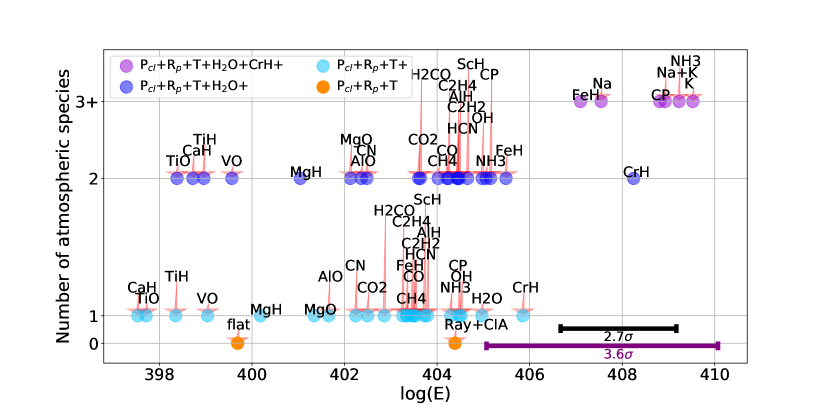
Figure 1: Model comparison for WASP-31b using Bayesian evidence for different atmospheric models. The flat model is shown as the orange dot, whereas cyan dots indicate higher complexity in the form of a chemical species, as labelled. One stage higher, blue dots represent a model that includes H₂O and an additional parameter. For the final stage, the strongest evidence model from lower complexities is complemented by K and potentially Na, as shown by the violet dots. In this final stage, we also tested the inclusion of some of the more likely species of lower levels. The horizontal scale bars indicate the statistical preference for a more complex model, based on Table 3.

At this stage, the strongest preference is found for the inclusion of either CrH or H₂O, with DSs over the flat model of $6.16$ and $5.28$, respectively. Following Jeffreys’ scale (see Table 3), this corresponds to confidence levels of ${\sim}3.9\sigma$ and ${\sim}3.7\sigma$, respectively. Compared to the model containing Rayleigh scattering and CIA, the CrH signature in this single-molecule model is detected at ${\sim}2.3\sigma$. Ascending one stage in complexity, the blue dots show the models consisting of H₂O and another species. It can be seen that the combined inclusion of both H₂O and CrH is preferred, with a DS of $8.56$ (or ${\sim}4.4\sigma$ confidence) over the flat model, or $3.86$ (${\sim}3.2\sigma$) over a model of only Rayleigh scattering and CIA. Compared to a CrH- or H₂O-only model, a model containing both species corresponds to confidence levels of ${\sim}2.6\sigma$ and ${\sim}3.0\sigma$, respectively.

The final stage is given by the violet dots and represents the addition of further atmospheric species to the best models of previous stages, in this case the one containing H₂O and CrH. Regarding the alkali metals, the inclusion of K in the WASP-31b atmospheric model is preferred, with a DS of 1.28 as compared to the H₂O+CrH model, whereas the model that includes both Na and K leads to a DS of 0.68. Hence, statistical evidence is only found for the absorption signature of K. The K detection corresponds to weak evidence at a confidence level of ${\sim}2.2\sigma$ over the H₂O$+$CrH model. The fact that the detection of K is mainly based on a single strong absorption peak can explain this weak evidence since the signature is covered by just a single data point. Naturally, providing a better fit to only one out of 63 data points may correspond to such a weak increase in Bayesian evidence. In this final stage, we also examined the individual additions of FeH, CP, and NH₃ to the H₂O$+$CrH model since these species correspond to the highest evidence levels in the previous stage, which included two atmospheric species. Compared to the H₂O$+$CrH model, the addition of NH₃ or CP leads to a small DS ($0.98$ and $0.56$, respectively) and the addition of FeH leads to a negative DS of ${-}1.15$. None of these are significant according to the Jeffreys’ scale.

Table 4: Resulting Bayesian evidence levels and DSs for WASP-31b. Except for the flat model, every model includes the opacity caused by Rayleigh scattering and CIA.

Model parameters	log(E)	DS
Flat model	399.69
Rayleigh + CIA	404.39	4.70
Compared to flat model
CaH	397.54	-2.16
TiO	397.72	-1.97
TiH	398.36	-1.34
VO	399.04	-0.65
MgH	400.19	0.50
MgO	401.35	1.66
AlO	401.66	1.97
CN	402.25	2.55
CO2	402.50	2.81
H2CO	402.86	3.17
C2H4	403.26	3.57
FeH	403.34	3.65
CH4	403.35	3.66
C2H2	403.46	3.77
CO	403.50	3.80
HCN	403.53	3.84
ScH	403.72	4.03
AlH	403.79	4.10
NH3	404.30	4.60
CP	404.48	4.78
OH	404.52	4.83
H2O	404.97	5.28
CrH	405.86	6.16
Compared to H2O-only model
H2O + TiO	398.38	-6.59
H2O + CaH	398.73	-6.24
H2O + TiH	398.96	-6.00
H2O + VO	399.57	-5.40
H2O + MgH	401.05	-3.92
H2O + MgO	402.13	-2.84
H2O + AlO	402.36	-2.61
H2O + CN	402.48	-2.48
H2O + CO2	403.60	-1.37
H2O + H2CO	403.64	-1.33
H2O + CH4	404.02	-0.95
H2O + CO	404.22	-0.75
H2O + C2H4	404.25	-0.72
H2O + HCN	404.44	-0.53
H2O + C2H2	404.44	-0.52
H2O + AlH	404.48	-0.49
H2O + ScH	404.66	-0.31
H2O + OH	404.98	0.01
H2O + NH3	405.06	0.09
H2O + CP	405.16	0.19
H2O + FeH	405.49	0.52
H2O + CrH	408.25	3.28
Compared to H2O+CrH model
H2O + CrH + FeH	407.10	-1.15
H2O + CrH + Na	407.55	-0.70
H2O + CrH + CP	408.81	0.56
H2O + CrH + Na + K	408.93	0.68
H2O + CrH + NH3	409.23	0.98
H2O + CrH + K	409.53	1.28

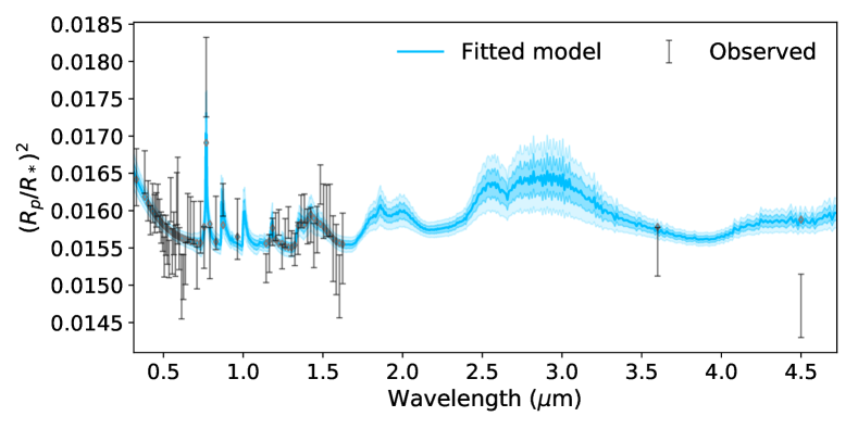
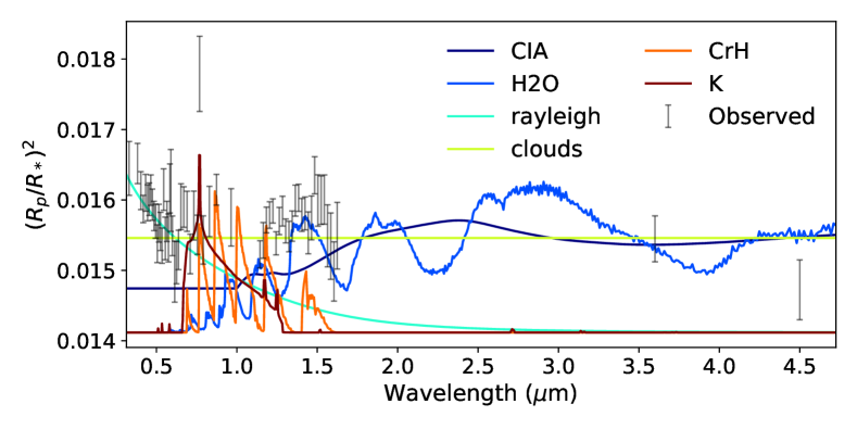
Figure 2: TauREx retrieval results for WASP-31b, with the transmission spectrum and the best-fitting atmospheric model (top) and the individual contributions of each molecule to the opacity (bottom). The vertical error bars indicate the observed transit depths, and the different shadings in the upper panel represent $1$ and $2{\sigma}$ regions.

We conclude that out of the models fitted in this study, the spectrum of WASP-31b is best represented by a model that includes H₂O, CrH, and K in addition to H₂, He, a grey cloud deck, and Rayleigh scattering. This atmospheric model and the observed transmission spectrum of WASP-31b are shown in the upper panel of Figure 2. The lower panel shows the individual contributions of the atmospheric constituents to the opacity. The signatures of H₂O in the near-infrared (around $1.0,1.2$, and $1.4\,\mu\mathrm{m}$; in blue) and K in the visible (around $0.77\,\mu\mathrm{m}$; dark red) are easily recognised, whereas the inclusion of CrH leads to the six absorption signatures between $0.7$ and $1.5\,\mu\mathrm{m}$, as shown by the orange line. On top of that, the navy line represents the continuum opacity provided by CIA, and the presence of aerosols results in two distinct signatures: the grey scattering opacity of a low altitude cloud deck and Rayleigh scattering at short wavelengths due to haze.

In Figure 2, a discrepancy can be seen between the transit depth resulting from our atmospheric model and the measured transit depth at $4.5\,\mu\mathrm{m}$ as observed by Spitzer. Uncertainties exist in cross-calibrating measurements by different instruments, and the usefulness of Spitzer’s broadband photometry in inferring atmospheric compositions has been called into question (see e.g. Hansen et al. 2014). To test our findings, we conducted the same analysis for a spectrum that excludes the Spitzer measurements. The spectrum and its best-fitting atmospheric model can be seen in Figure 3. Excluding the Spitzer measurements leads to a significant preference for the CrH+H₂O model, with confidence levels of ${\sim}4.8\sigma$ over a flat model and ${\sim}3.9\sigma$ over a model containing Rayleigh scattering and CIA. Besides that, the retrieved values are consistent with our earlier findings within $1\sigma$. Therefore, we conclude that removing the Spitzer measurements does not change our results significantly, illustrating that mid-infrared coverage is not required to detect CrH. The discrepancy between the data and our model at these wavelengths hints at the influence of species that show spectral activity in these regions (such as CO and CO₂).

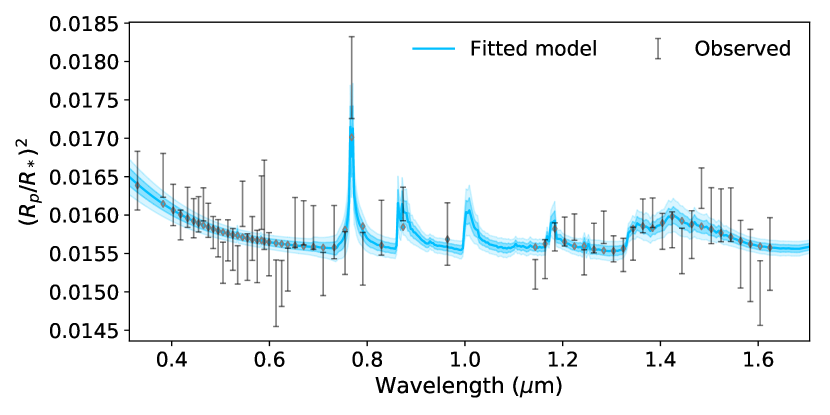
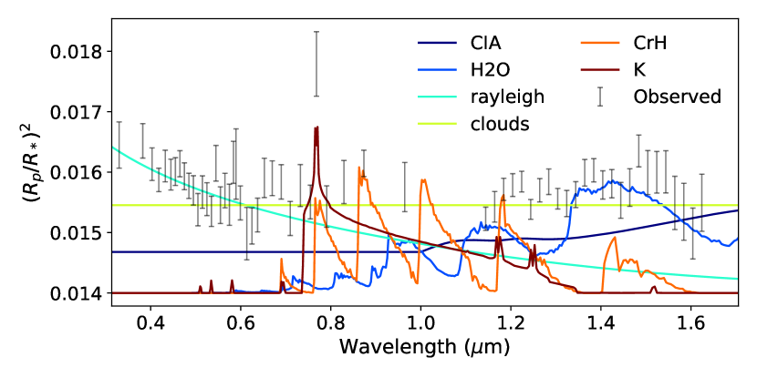
Figure 3: TauREx retrieval results for WASP-31b without the Spitzer measurements.

4 Discussion

Before discussing the retrieved parameters, it is important to emphasise that the resulting atmospheric parameters are based on the models that turned out to be the best fit to the spectral data of WASP-31b. A bottom-up approach is valuable in inferring the presence of chemical species in an atmosphere but may lead to biases in the derived constraints on retrieved parameters. Excluding a particular chemical species from the atmospheric model means that the spectroscopic signature of the species has not been detected on the basis of statistics. This does not necessarily mean that a chemical species is completely absent from the atmosphere that is probed. Instead, the signatures of a species can fall outside of the observed spectral range, be too weak to be detected, or be affected by an overlap with other spectral signatures. The omission of a particular species can then influence the retrieval outcomes since its signatures (even if they are statistically insignificant) have to be explained by the absorption of other species. This may result in unreasonably tight constraints as well as unrealistic values for retrieved abundances. In this way, the retrievals may introduce biases in, for example, the abundances of species that are included in the model. The retrieved parameters for our best-fitting model are shown in Table 5, and the extended posterior distributions can be found in Figure A of the appendix. To test whether the omission of atmospheric species leads to biases in the retrieved parameters, we retrieved the same spectrum assuming a model with a variety of opacity sources (H₂O, CrH, K, CO₂, CO, CH₄, NH₃, and Na). This retrieval results in similar abundances of $\log(\mathrm{X_{H_{2}O}}){=}{-}5.39^{+0.42}_{-0.73}$, $\log(\mathrm{X_{CrH}}){=}{-}8.19^{+0.75}_{-0.77}$, and $\log(\mathrm{X_{K}}){=}{-}7.92^{+0.82}_{-1.59}$ (see the second row of Table 9). This shows that including the other chemical species is not essential when retrieving abundances from this spectrum of WASP-31b. Increasing the number of opacity sources leads to a larger error on the retrieved parameters. This is as expected: Widening the allowed parameter space increases the number of possible solutions in the retrieval procedure.

Table 5: Retrieved atmospheric parameters using TauREx for the model shown in Figure 2. The extended posterior distributions can be found in Figure A of the appendix.

Parameter	Retrieved value
T${}_{\mathrm{atm}}\,(\mathrm{K})$	$1481^{+264}_{-355}$
$\mathrm{R_{pl}}\,(\mathrm{R_{J}})$	$1.48^{+0.02}_{-0.01}$
$\log(\mathrm{P_{clouds}})\,(\mathrm{Pa})$	$3.87^{+0.20}_{-0.20}$
$\log(\mathrm{X_{H_{2}O}})$	$-5.40^{+0.37}_{-0.43}$
$\log(\mathrm{X_{CrH}})$	$-8.51^{+0.62}_{-0.60}$
$\log(\mathrm{X_{K}})$	$-7.59^{+0.66}_{-0.94}$

4.1 Comparison to previous work

Earlier investigations of the transmission spectrum of WASP-31b found signatures of K, a grey cloud deck, and Rayleigh scattering (Sing et al. 2015, 2016). On top of that, a weak water absorption feature was found, which was also reported by later studies that used the same spectrum (Barstow et al. 2017; Tsiaras et al. 2018). Tsiaras et al. (2018) found weak evidence for a water VMR of $\log(\mathrm{X_{H_{2}O}}){=}-3.84\pm 1.90$. Other retrieved water abundances are equal to $-3.97^{+1.01}_{-2.27}$ (Pinhas et al. 2019) and $-4.55^{+1.77}_{-4.33}$ (Welbanks et al. 2019) with confidence levels of ${\sim}2\sigma$ and ${\sim}2.2\sigma$, respectively, and an abundance of $-3.27^{+1.44}_{-2.18}$ is found using the classical retrieval method within the ARCiS code (Min et al. 2020). Our retrieved water abundance (see Table 5) is lower but falls inside the error bars of the other investigations. Sing et al. (2015) reported a $4.2\sigma$ significant detection of K, but the fidelity of this data point was later questioned by individual searches using the ground-based facilities FORS2 and UVES (Gibson et al. 2017, 2019) and IMACS (McGruder et al. 2020). Our detection agrees with the $2.2\sigma$ detection that was made using combined FORS2 and STIS optical data (Gibson et al. 2017). MacDonald & Madhusudhan (2017) also found a weak detection ($2.2\sigma$) of NH₃, which was found at a similar abundance by Min et al. (2020). As can be seen in Table 4, the addition of NH₃ to our H₂O+CrH model also leads to an increase in the evidence level (DS${=}0.98$). As shown in Table 3, this was not seen as significant in our analysis (just below $2.1\sigma$). This small difference can be explained by the overlap in the CrH and NH₃ features around $1.5\,\mu\mathrm{m}$. Covering the features at longer wavelengths (e.g. at ${\sim}2.2\,\mu\mathrm{m}$) will greatly improve our ability to detect NH₃, as illustrated by MacDonald & Madhusudhan (2017).

Retrieved atmospheric temperatures for WASP-31b vary from $738^{+345}_{-231}\,\mathrm{K}$ (Min et al. 2020) to $1088.35\pm 220.16\,\mathrm{K}$ (Tsiaras et al. 2018) and $1043^{+267}_{-172}\,\mathrm{K}$ (Pinhas et al. 2019), all of which are exceeded by our retrieved temperature. Moreover, MacDonald et al. (2020) showed that hot Jupiter temperatures are generally underestimated by 1D retrievals. An explanation for this discrepancy in temperature might be an insufficient cloud model since Sing et al. (2016) reported that the spectrum of this planet is not well explained by a single cloud model. A more complex model is included in TauREx, which parametrises the opacity caused by particle scattering following the Mie theory (Lee et al. 2013). Adding this parametrisation to our best-fitting model also results in a relatively high $\mathrm{T_{atm}}{=}1507^{+239}_{-308}\,\mathrm{K}$ and low $\log(\mathrm{X_{H_{2}O}}){=}-5.73^{+0.51}_{-3.77}$ and is not found to be statistically significant. It is possible that this parametrisation is still not sufficiently complex. Another explanation may be the difference in opacity sources that are included: Our retrieval only includes H₂O, CrH, and K, whereas the others generally include H₂O, CH₄, CO, CO₂, and NH₃. Additionally, Na and K (Pinhas et al. 2019; Min et al. 2020) and HCN (Pinhas et al. 2019) were also included in the retrievals. Increasing the number of opacity sources does indeed lead to a lower temperature of $\mathrm{T_{atm}}{=}1172^{+435}_{-226}\,\mathrm{K}$ (see the second row of Table 9), consistent with the majority of earlier findings. With a Bayesian evidence level of 407.61, the addition of these opacity sources is not found to be statistically significant.

Associated with the lower temperature of this retrieval is an increase in the retrieved radius to $1.50\,\mathrm{R_{J}}$. As shown in Table 5, the radius of WASP-31b is equal to $1.48\,\mathrm{R_{J}}$ in our best-fit model. This degeneracy between $\mathrm{R_{pl}}$ and T can also be seen from the posterior distributions in Figure A: Specifically, the plot in row 3 (from the bottom) and column 4 (from the left) shows that an increase in radius is degenerate with a decrease in temperature (due to its influence on the scale height). This degeneracy is another explanation for the difference with Min et al. (2020), who retrieve $\mathrm{R_{pl}}{=}1.51^{+0.02}_{-0.03}\,\mathrm{R_{J}}$. To test this suspicion, a retrieval was conducted assuming a fixed radius of $\mathrm{R_{pl}}{=}1.549$, and it did indeed result in a lower temperature of $1267^{+351}_{-288}\,\mathrm{K}$. However, this result is accompanied by unphysically high abundances of CrH and K (${\log(\mathrm{X})}{=}{-}3.61$ and ${-}0.18$, respectively). Using equilibrium temperatures, we can predict the maximum temperature of the terminator region to be ${\sim}1550\,\mathrm{K}$ for full redistribution ($f{=}1$) and perfect absorption of radiation ($A{=}0$). Hence, our retrieved temperature would be reasonable. The degeneracy that exists between temperature, radius, and abundances (e.g. Griffith 2014; Heng & Kitzmann 2017) may offer an explanation for the relatively low water abundances that we retrieve. A higher temperature leads to an overall increase in the scale height and thus the transit depth, dampening absorption features and leading to lower chemical abundances in the retrieval.

Previous identifications of the signatures of CrH have been reported for brown dwarfs (e.g. Kirkpatrick et al. 1999a, b). Specifically, Burrows et al. (2002) found an abundance of $\mathrm{CrH/H_{2}}{\sim}2{-}4{\times}10^{-9}$ for the L5 dwarf 2MASSI J1507038-151648, which is in excellent agreement with the abundance that we retrieve for WASP-31b. MacDonald & Madhusudhan (2019) report a $4.1{\sigma}$ detection of metal hydrides in the transmission spectrum of exo-Neptune HAT-P-26b, and they identify three possible candidates: TiH ($4.1{\sigma}$), CrH ($2.1{\sigma}$), or ScH ($1.8{\sigma}$). As a possible candidate, CrH is retrieved at an abundance of $-5.72^{+0.89}_{-1.37}$, which exceeds our value by almost three orders of magnitude. They propose vertical transport or secular contaminations by planetesimals as possible explanations for this high abundance and the fact that Cr is expected to have condensed out at the temperature of HAT-P-26b ($\mathrm{T_{eq}{\sim}1000}\,\mathrm{K}$).

The retrieved abundances can also be compared to the predictions from equilibrium chemistry, for example by using the GGChem code (Woitke et al. 2018). Around our retrieved temperature of WASP-31b, GGChem predicts CrH to be present at $\log(\mathrm{X_{CrH}}){\sim}{-}9$ for $\mathrm{P}{=}1\,\mathrm{bar}$ and solar composition, with lower abundances for lower pressures (Woitke et al. 2018). Hence, the retrieved CrH abundance of $-8.51^{+0.62}_{-0.60}$ is higher than predicted but still consistent. H₂O is expected at $\log(\mathrm{X_{H_{2}O}}){\sim}{-}3.3$ for the same temperature, about 100 times higher than the retrieved abundance. As previously stated, this might be related to degeneracies between different retrieval parameters. The fact that this large difference is not retrieved for the CrH abundance might also hint at an actual depletion of H₂O. Further observations can help in disclosing this.

4.2 Chemistry

From the first-row transition metals, Cr is the third most abundant element after Fe and Ni in the Sun (Asplund et al. 2009). At the temperatures of close-in exoplanets, CrH is predicted to be an important Cr-bearing species. However, gaseous atomic Cr is expected to be the main Cr bearer, whereas significant fractions are also expected to be present in CrO or CrS (Woitke et al. 2018). These calculations were made assuming solar abundances and the corresponding solar abundance ratio $\log(\mathrm{Cr/O}){=}-3.05$ (Asplund et al. 2009). If we make the simplifying assumption that for WASP-31b most of the Cr is in CrH, the planetary $\mathrm{Cr/O}$ abundance ratio can be calculated. At the temperature of WASP-31b, about half of the oxygen is expected in H₂O and the other half in CO (Madhusudhan 2012; Woitke et al. 2018). To correct for this, the retrieved H₂O abundance is multiplied by two, leading to a ratio of $\log(\mathrm{Cr/O}){=}{-}3.41$. The abundance ratio is lower than the solar value, but additional Cr is probably present in other species. Including the opacity data of these species in retrievals can lead to better constraints on the ratios, and the detectability of atomic Cr has recently been shown by its signatures in the ultra-hot Jupiter WASP-121b (Ben-Yami et al. 2020). Of course, abundance ratios may differ per star. For WASP-31, ratios are measured to be $\mathrm{O/H}{=}{+}0.06\,\mathrm{dex}$ and $\mathrm{Cr/H}{=}{-}0.08\,\mathrm{dex}$, relative to the Sun (Brewer et al. 2016). This leads to a lower stellar abundance ratio of $\log(\mathrm{Cr/O}){=}{-}3.19$ for WASP-31, which may also partly explain the lower planetary ratio.

Monatomic Cr, the major gas-phase bearer at a wide range of temperatures ($300-3000$ K), is a refractory species. At the relevant pressures, it condenses into Cr metal between $1400$ and $1520$ K and into Cr₂O₃ at lower pressures of ${\sim}10^{-3}$ bar (e.g. Burrows & Sharp 1999; Lodders & Fegley 2006; Morley et al. 2012). The CrH abundance is related to the monatomic gas according to the equilibrium (Lodders & Fegley 2006):

$$\ce{2Cr(g)+H$_{2}$<=>2CrH(g).}$$ (3)

The condensation of Cr metal reduces the abundances of monatomic Cr and CrH, depleting the species from the atmosphere. Vertical mixing from lower, hotter layers is unlikely since Cr destruction reactions are highly exothermic at $\mathrm{T}{<}1400\,\mathrm{K}$, resulting in chemical lifetimes much shorter than the timescales of vertical mixing (Lodders & Fegley 2006). For the WASP-31b $\mathrm{T_{atm}}{=}1481^{+264}_{-355}\,\mathrm{K}$, the appearance of CrH would be reasonable since the gaseous Cr would not yet be fully depleted.

The discovery of Cr bearers can have implications for cloud formation in exoplanet atmospheres since they may cause the formation of Cr[s] clouds (Lodders & Fegley 2006; Morley et al. 2012). Moreover, Lee et al. (2018) suggested the possibility of Cr[s] being seed particles that provide condensation surfaces for other cloud layers (e.g. sulphide or KCl cloud layers).

Lastly, the finding of Cr-bearing species in an atmosphere may give clues about the formation conditions of a planet. Because Cr is a refractory species, it is expected to be in the solid phase throughout most of the protoplanetary disk (e.g. Lodders 2010). Consequently, its presence on an exoplanet hints at the accretion of solid material during its formation. Determining the planetary Cr abundance (also in other Cr bearers) can then provide clues about the amount of solid accretion.

4.3 Other observations

Since the fidelity of the data point responsible for the K detection has been questioned (Gibson et al. 2017, 2019), a few retrievals were conducted excluding the observed transit depth at ${\sim}0.77\,\mu\mathrm{m}$. CrH has absorption features around this wavelength, and these retrievals were done to make sure that the tentative CrH detection is not based on a disputed observation. A similar approach to what was described in Section 2 was followed. The resulting Bayesian evidence levels can be seen in Table 6 and agree with our earlier findings, albeit with slightly lower DSs: The inclusion of both H₂O and CrH is preferred, with a DS of $7.97$ (or ${\sim}4.3\sigma$ confidence) over the flat model, or $2.98$ (${\sim}2.9\sigma$) over a model of only Rayleigh scattering and CIA. The influence of the measured transit depth at ${\sim}0.77\,\mu\mathrm{m}$ is explained by this decrease in DS, but, even without the measurement, statistically significant evidence for CrH is still found. In this case, a slightly lower $\mathrm{T_{atm}}{=}1339^{+332}_{-321}\,\mathrm{K}$ and higher $\mathrm{R_{pl}}{=}1.49^{+0.02}_{-0.02}\,\mathrm{R_{J}}$ are retrieved.

Table 6: Resulting Bayesian evidence levels and DSs for the Sing et al. (2015) spectrum without $0.77\,\mu\mathrm{m}$ observation.

Model parameters	log(E)	DS
Flat model	400.44
Rayleigh+CIA	405.43	4.99
Compared to flat model
CrH	406.01	5.58
CrH+H2O	408.40	7.97

Ground-based optical data by the FORS2 at the VLT are also available for this planet (Gibson et al. 2017) and offer coverage from $0.4$ to $0.84\,\mu\mathrm{m}$. The combined FORS2/STIS data that are presented by Gibson et al. (2017) were also analysed using TauREx. With the same general setup, we retrieved the spectrum assuming five different models to test whether the CrH features are also found in the ground-based data. The resulting evidence levels and accompanying DSs are shown in Table 7. Using these data, a model containing CrH is not found to be statistically significant over a model only containing Rayleigh scattering and CIA. Hence, in this case, the best-fitting atmospheric model was found to consist only of Rayleigh scattering and CIA and to be without any chemical species, indicating a cloudy atmosphere at a retrieved temperature of $\mathrm{T_{atm}}{=}1503^{+267}_{-369}\,\mathrm{K}$. The retrieved planetary radius agrees with the value we previously found at $1.48^{+0.02}_{-0.01}\,\mathrm{R_{J}}$. The spectrum and its lack of absorption features can be seen in Figure 4. While the measured transit depths between $0.7$ and $1.0\,\mu\mathrm{m}$ seem to show some signatures, they are not found to be statistically significant. For comparison, the forward model based on the retrieved parameters in Table 5 is shown by the red line, indicating the signatures that should be visible when CrH is present in the atmosphere.

Table 7: Resulting Bayesian evidence levels and DSs for the combined FORS2/STIS data.

Model parameters	log(E)	DS
Flat model	241.49
Rayleigh+CIA	245.36	3.87
Compared to flat model
CrH+K	244.56	3.08
CrH	244.72	3.24
CrH+H2O	245.50	4.01

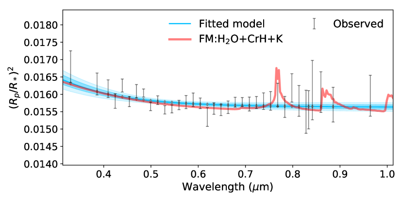
Figure 4: Transmission spectrum as observed by FORS2/STIS with the best-fitting atmospheric model. The vertical error bars indicate the observed transit depths, and the different shadings in the upper panel represent $1$ and $2{\sigma}$ regions. A forward model based on the retrieval results in Table 5 is shown by the red line.

Taking another look at the bottom image of Figure 3, the orange line shows that the presence of CrH results in six prominent absorption peaks. Only three of these peaks (at $0.69$, $0.77$, and $0.88\,\mu\mathrm{m}$) fall (partially) inside the range probed by this combined FORS2/STIS spectrum, which can also be seen from the red line in Figure 4. To test whether the peaks in the WFC3 regime (at $1.18$ and $1.43\,\mu\mathrm{m}$) are driving the evidence for CrH, we added the WFC3 data to the combined FORS2/STIS data and conducted some additional retrievals on this spectrum. From the resulting evidence levels, as shown in Table 8, it can be seen that this does not lead to a significant detection of CrH and only results in a preference for H₂O at ${\sim}3.7\sigma$ over a flat model. Using this spectral coverage, the temperature is retrieved to be $\mathrm{T_{atm}}{=}1476^{+277}_{-376}\,\mathrm{K}$ and the planetary radius agrees with our earlier findings at $1.48^{+0.02}_{-0.02}\,\mathrm{R_{J}}$. We can conclude that the evidence for CrH is driven by the observations made with STIS, specifically the observed transit depths around $0.88$ and $0.77\,\mu\mathrm{m}$. However, compatibility between different instruments cannot be taken for granted, and caution should thus be exercised when combining data, as illustrated by Hou Yip et al. (2020) for the case of WASP-96b. This uncertainty, the non-detection when including ground-based data, and the broad continuous wavelength coverage that will be offered by future facilities further motivate the characterisation of WASP-31b.

Table 8: Resulting Bayesian evidence levels and DSs for a combined FORS2/STIS and WFC3 spectrum.

Model parameters	log(E)	DS
Flat model	408.37
Rayleigh+CIA	412.69	4.32
Compared to flat model
FeH	410.81	2.45
CrH	411.60	3.23
H2O	413.91	5.55
Compared to H2O-only model
H2O + FeH	412.60	-1.31
H2O + AlH	412.86	-1.05
H2O + CP	413.23	-0.68
H2O + CrH	413.29	-0.62
H2O + ScH	413.37	-0.55
H2O + NH3	414.19	0.28

4.4 Near-future coverage

Figure 5 shows the transmission spectrum for the wider wavelength range offered by the James Webb Space Telescope (JWST), scheduled for launch in October 2021. Using a variety of instruments, JWST will offer a spectral range from $0.6$ to $28\,\mu\mathrm{m}$ (Beichman et al. 2014). The spectra in Figure 5 correspond to different atmospheric compositions and are based on forward models that assume the retrieved best-fit values for atmospheric parameters; because of the discrepancy in the K detection, the alkali metal is not included in the models.

The blue model is the only forward model that does not include CrH, and, by comparing it with the other models, it can be seen that the presence of CrH is purely based on the absorption signatures between $0.69$ to $1.43\,\mu\mathrm{m}$. Next to that, the presence of water can clearly be inferred from the familiar feature around $1.4\,\mu\mathrm{m}$ as well as the feature at $1.9\,\mu\mathrm{m}$, showing a clear distinction from the CrH-only model. Although many additional water signatures can be found at longer wavelengths, the fact that JWST’s Near Infrared Imager and Slitless Spectrograph (NIRISS) can provide simultaneous coverage at $\mathrm{R}{\sim}700$ from $1$ to $2.5\,\mu\mathrm{m}$ makes these H₂O features and the CrH features in this regime interesting prospects for further characterisation. Another important goal is to derive improved C/O ratios, and combined observations from NIRISS and the Near Infrared Camera (NIRCam) are expected to deliver this (Stevenson et al. 2016), providing coverage from $1$ to $5\,\mu\mathrm{m}$. This is also evident from Figure 5, where a variation in transit depth can be seen around wavelengths of $4.5\,\mu\mathrm{m}$, depending on whether or not CO or CO₂ are included in the forward model. Hence, WASP-31b would be an interesting target for further characterisation, whereas the presence of CrH (and other metal hydrides) in exoplanets of similar temperatures is expected to be detectable with JWST. Because CrH rapidly condenses out for lower temperatures and the spectral signatures of more refractory materials such as TiO and VO start taking over at higher temperatures, its presence is probably detectable for planets with temperatures ranging from ${\sim}1300{-}2000\,\mathrm{K}$.

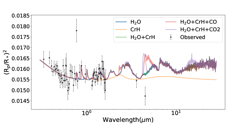
Figure 5: Forward models for the transmission spectrum of WASP-31b in the spectral regime of JWST, based on the retrieved values for atmospheric parameters in Table 5.

5 Conclusions

In this study, a re-analysis of publicly available transmission data of the hot exoplanet WASP-31b has been conducted using the TauREx II retrieval framework. Transmission data from STIS, WFC3, and Spitzer provide spectral coverage between $0.3$ and $4.5\,\mu\mathrm{m}$. Assuming the simplified atmospheric representation in TauREx and out of the models that were fitted in this analysis, it was found that the spectrum is best explained by a model containing H₂O, CrH, and K in addition to H₂, He, a grey cloud deck, and Rayleigh scattering. As compared to a flat model without any spectral features, the H₂O-only model is statistically preferred at ${\sim}3.7\sigma$ and a CrH-only model at ${\sim}3.9\sigma$. A model with both H₂O and CrH was found at ${\sim}4.4\sigma$ and ${\sim}3.2\sigma$ over the flat model and a CIA+Rayleigh scattering model, respectively. Hence, we report the first statistical evidence for the signatures of CrH in an exoplanet atmosphere. Weak evidence for the addition of K to the atmospheric model was found at ${\sim}2.2\sigma$ confidence over the H₂O+CrH model. As compared to earlier studies of WASP-31b, a relatively high temperature was retrieved, which can be explained by a combined influence of fewer opacity sources and degeneracies between temperature, radius, and chemical abundances.

The evidence for CrH naturally follows from its presence in brown dwarfs and is expected to be limited to planets with temperatures between $1300$ and $2000\,\mathrm{K}$. Cr-bearing species may play a role in the formation of clouds in exoplanet atmospheres, and their detection is also an indication of the accretion of solids during the formation of a planet.

In additional retrievals, the disputed data point at ${\sim}0.77\,\mu\mathrm{m}$ was excluded, but evidence for the H₂O+CrH model was still found at a confidence level of ${\sim}4.3\sigma$ over the flat model. A combined FORS2/STIS spectrum was also available and tests were performed to confirm the CrH detection, but in this case no statistically significant CrH feature was found. By analysing the retrieval outcomes for different combinations of spectral coverage, it was found that the evidence for CrH is mostly based on the observed transit depths around $0.77$ and $0.88\,\mu\mathrm{m}$. Inspired by the non-agreement between different instruments, and using the best-fit atmospheric model for WASP-31b, it was shown that the spectral regime of JWST has the potential to confirm the CrH features.

Appendix A Retrieval outputs

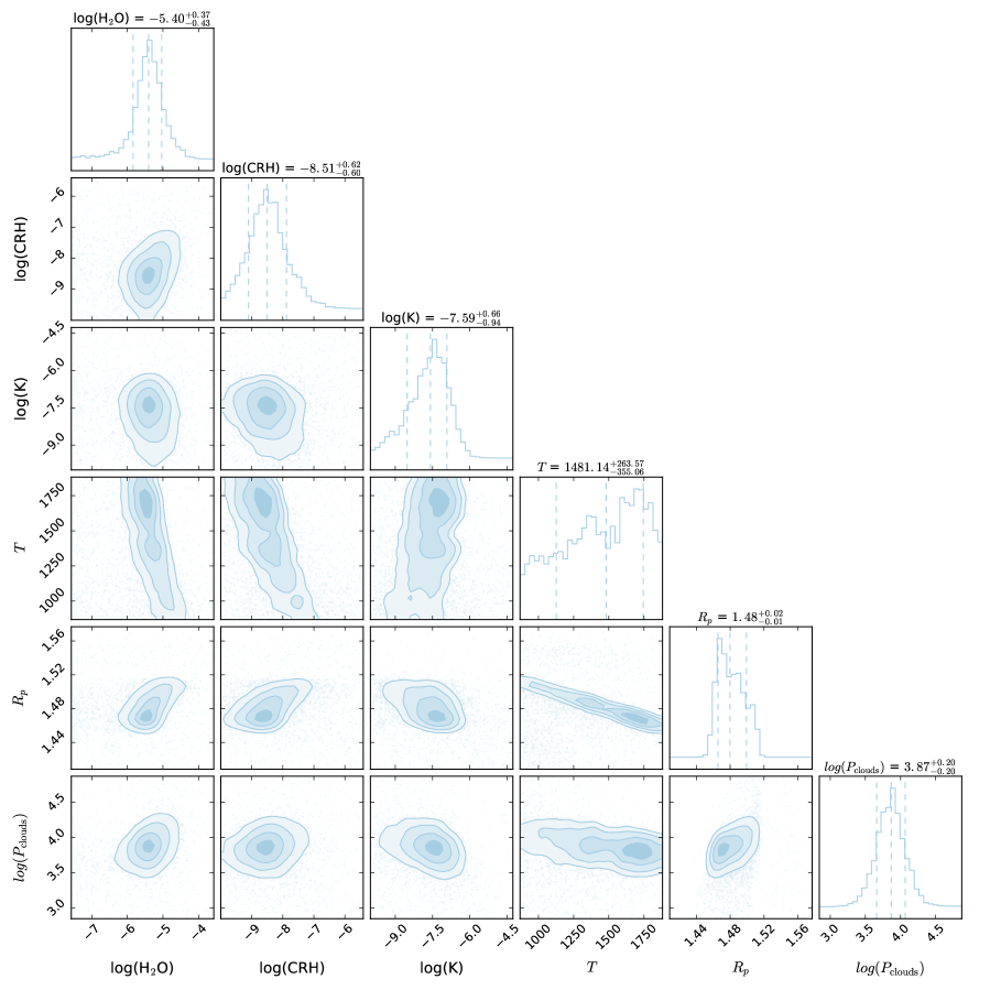
Figure 6: TauREx posterior distributions of highest evidence retrieval for WASP-31b.

Table 9: Retrieved atmospheric parameters using TauREx for different retrieval setups and spectral coverage. We note that, besides the setups described here, the models also include H₂, He, a grey cloud deck, and Rayleigh scattering.

Coverage and retrieval setup	T${}_{\mathrm{atm}}\,(\mathrm{K})$	$\mathrm{R_{pl}}\,(\mathrm{R_{J}})$	$\log(\mathrm{P_{clouds}})\,(\mathrm{Pa})$	$\log(\mathrm{X_{H_{2}O}})$	$\log(\mathrm{X_{CrH}})$	$\log(\mathrm{X_{K}})$
STIS + WFC3 + Spitzer
H2O+CrH+K (highest Evidence model)	$1481^{+264}_{-355}$	$1.48^{+0.02}_{-0.01}$	$3.87^{+0.20}_{-0.20}$	$-5.40^{+0.37}_{-0.43}$	$-8.51^{+0.62}_{-0.60}$	$-7.59^{+0.66}_{-0.94}$
H2O+CrH+K+CO2+CO+CH4+NH3+Na	$1172^{+435}_{-226}$	$1.50^{+0.01}_{-0.02}$	$4.03^{+1.07}_{-0.29}$	$-5.39^{+0.42}_{-0.73}$	$-8.19^{+0.75}_{-0.77}$	$-7.92^{+0.82}_{-1.59}$
H2O+CrH+K (Complex cloud)	$1507^{+239}_{-308}$	$1.48^{+0.02}_{-0.01}$	$3.86^{+0.18}_{-0.19}$	$-5.41^{+0.33}_{-0.37}$	$-8.53^{+0.57}_{-0.58}$	$-7.63^{+0.67}_{-0.87}$
H2O+CrH+K (Radius fixed at 1.549$\,\mathrm{R_{J}})$	$1267^{+351}_{-288}$	$1.549^{+0.00}_{-0.00}$	$0.93^{+0.98}_{-1.27}$	$-5.25^{+3.46}_{-3.20}$	$-3.61^{+2.40}_{-3.26}$	$-0.18^{+0.11}_{-0.18}$
H2O+CrH	$1339^{+332}_{-321}$	$1.49^{+0.02}_{-0.02}$	$3.89^{+0.22}_{-0.21}$	$-5.33^{+0.44}_{-0.44}$	$-8.45^{+0.66}_{-0.63}$	n/a
STIS + WFC3
H2O+CrH+K	$1614^{+184}_{-309}$	$1.47^{+0.02}_{-0.01}$	$3.86^{+0.18}_{-0.19}$	$-5.35^{+0.29}_{-0.28}$	$-8.65^{+0.56}_{-0.56}$	$-7.54^{+0.64}_{-0.84}$
FORS2/STIS
No species	$1503^{+267}_{-369}$	$1.48^{+0.02}_{-0.01}$	$3.66^{+0.18}_{-0.23}$	n/a	n/a	n/a
FORS2/STIS + WFC3
H2O	$1476^{+277}_{-376}$	$1.48^{+0.02}_{-0.01}$	$3.76^{+0.17}_{-0.21}$	$-5.51^{+0.38}_{-0.75}$	n/a	n/a