Born Identity Network:
Multi-way Counterfactual Map Generation to Explain a Classifier’s Decision

Abstract

There exists an apparent negative correlation between performance and interpretability of deep learning models. In an effort to reduce this negative correlation, we propose a Born Identity Network (BIN), which is a post-hoc approach for producing multi-way counterfactual maps. A counterfactual map transforms an input sample to be conditioned and classified as a target label, which is similar to how humans process knowledge through counterfactual thinking. For example, a counterfactual map can localize hypothetical abnormalities from a normal brain image that may cause it to be diagnosed with a disease. Specifically, our proposed BIN consists of two core components: Counterfactual Map Generator and Target Attribution Network. The Counterfactual Map Generator is a variation of conditional GAN which can synthesize a counterfactual map conditioned on an arbitrary target label. The Target Attribution Network provides adequate assistance for generating synthesized maps by conditioning a target label into the Counterfactual Map Generator. We have validated our proposed BIN in qualitative and quantitative analysis on MNIST, 3D Shapes, and ADNI datasets, and showed the comprehensibility and fidelity of our method from various ablation studies. Code is available at: https://github.com/ksoh97/BIN.

1 Introduction

As deep learning has shown its success in various domains, there has been a growing need for interpretability and explainability in deep learning models. The black-box nature of deep learning models limits their real-world applications in fields, especially, where fairness, accountability, and transparency are essential. Moreover, from the end-user point of view, it is a crucial process that requires a clear understanding and explanation at the level of human knowledge. However, achieving high performance with interpretability is still an unsolved problem in the field of explainable AI (XAI) due to their apparent negative correlation [19] (i.e. interpretable models tend to have a lower performance than black-box models).

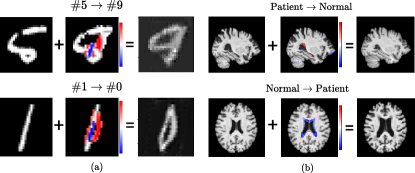
Figure 1: We propose an approach for producing counterfactual maps as a step towards counterfactual reasoning, which is a process of producing hypothetical realities given observations. For example, a counterfactual map can localize hypothetical, yet very possible, abnormalities from a brain image of a normal subject that may cause the subject to be diagnosed with a disease.

Reducing this negative correlation in performance and interpretability has been a long-standing goal in the field of XAI. In the early era of XAI [15], researchers have proposed various methods for discovering or identifying the regions that have the most influence on deriving the outcome of the classifier [32, 37, 38, 1, 28, 33, 35, 42]. The main objective of these early era XAI methods is to answer why and how a model has made its decision. However, recent XAI methods induce to answer the question that can offer a more fundamental explanation: “What are the hypothetical alternative scenarios that may have altered the outcome?”. This sort of explanation is defined at the root of counterfactual reasoning. Counterfactual reasoning can provide an explanation at the level of human knowledge since it can explain a model’s decision in hypothetical situations. Thus, we propose to show a higher-level visual explanation of a deep learning model similar to that of how humans process knowledge, i.e., through the means of a counterfactual map.

A counterfactual map is a map that can transform an input sample that was originally classified as one label to be classified as another. For example, a counterfactual map transforms a digit image to be an image of another number (Figure 1-(a)). This counterfactual map explains what kind of structural changes are required for a digit image to be another number with the least amount of modification to the original image. A real-world application can be of a medical image analysis of the brain (Figure 1-(b)), where a counterfactual map would describe which Region Of Interests (ROIs) may cause a normal subject to be diagnosed with a disease (also with least amount of modification to the original image).

To our knowledge, most works on producing counterfactual explanations are generative models. Most notably, these works utilize Generative Adversarial Network (GAN) and its variants [16, 6, 39, 9, 31] to synthesize a counterfactual explanation. Although these works can generate meaningful counterfactual explanations, two fundamental problems limit their application in the real-world. First, generative models are a typical example of models that experience the aforementioned negative correlation between performance and interpretability. To address this issue, we propose a method that can produce counterfactual maps from a pre-trained model (i.e., we can focus solely on interpretability with the higher performance given beforehand).

Second, recent works on counterfactual explanation can only produce a single-[9, 16, 6] or dual-[17, 40] way explanation. In other words, they only consider one or two hypothetical scenarios for counterfactual reasoning (e.g., single-way counterfactual map can only transform a normal subjects to Alzheimer’s disease patients, and vice versa for dual-way maps). With the help of a target attribution mechanism, our work, to the best of our knowledge, is the first to propose a multi-way counterfactual reasoning (e.g., producing maps that can freely transform any image samples to or from normal subject, mild cognitive impairment patient, and Alzheimer’s disease patient).

The motivation behind a multi-way counterfactual map is (in contrast to single-/dual-way) the stratification of hypothetical alternatives, especially in the medical domain. A single-/dual-way counterfactual map is only able to justify the outcome in one or two extreme tails (e.g., disease or normal), while in real-world, diseases are usually stratified by the severity and/or progression. A multi-way counterfactual map provides a natural proxy for stratification of diseases by providing hypothetical scenarios for prodromal stages (i.e., preceding stages) of a disease.

To this end, we propose Born Identity Network (BIN) that produces a counterfactual map using two components: The Counterfactual Map Generator (CMG), and the Target Attribution Network (TAN). The CMG is a variant of conditional GAN [27] that synthesizes a conditioned map, while the TAN provides adequate assistance to the CMG by enforcing a target counterfactual attribute to the synthesized conditioned map. We have validated our proposed BIN in qualitative and quantitative analysis on MNIST, 3D Shapes, and ADNI datasets, and showed the comprehensibility and fidelity of our method from various ablation studies.

The main contributions of our study are as follows:

• We propose Born Identity Network (BIN), which, to the best of our knowledge, is the first work on producing counterfactual reasoning in multiple hypothetical scenarios.

• A Multi-way counterfactual map can provide a more precise explanation which accounts for severity and/or progression of a disease.

• BIN is a generalized interpretation model which can be plugged-in to most pretrained neural networks without any modification to the weights of the pretrained model.

2 Related Works

In this section, we describe various works proposed for explainable AI (XAI). First, we divide XAI into a general framework of attribution-based explanation and a more recent framework of counterfactual explanation. Second, we have compared different approaches to counterfactual explanation in the Supplementary.

2.1 Attribution-based Explanations

Attribution-based explanation refers to discovering or identifying the regions that have the most influence on deriving the outcome of a model. These approaches can further be separated into the gradient-based and reference-based explanation. First, the gradient-based explanation highlights the activation nodes that most contributed to the model’s decision. For example, Class Avtivation Map (CAM) [43], and Grad-CAM [32] highlight activation patterns of weights in a specified layer. In a similar manner, DeepTaylor [28], DeepLift [33], and Layer-wise Relevance Propagation (LRP) [1] highlight the gradients with regard to the prediction score. These approaches usually suffer from vanishing gradients due to the ReLU activation, and Integrated Gradients [38] resolves this issue through sensitivity analysis. However, a crucial drawback of attribution-based approaches is that they tend to ignore features with relatively low discriminative power or highlight only those with overwhelming feature importance. Second, the reference-based explanation [42, 13, 6, 11] focuses on changes in model output with regards to perturbation in input samples. Various perturbation methods, such as masking [8], heuristic [6] (e.g., blurring, and random noise), region of the distractor image as reference for perturbation [17], or synthesized perturbation [11, 42, 13], has been proposed. One general drawback of these aforementioned attribution-based explanations is that they tend to produce low-resolution and blurred salient map. In contrast, our work can produce a crisp salient map with the same resolution as the input sample using a GAN.

2.2 Counterfactual Explanations

Recently, more researchers have focused on counterfactual reasoning as a form of higher-level explanation. Counterfactual explanation refers to analyzing the model’s output with regards to hypothetical scenarios. For example, a counterfactual explanation could highlight those regions that may (hypothetically) cause a normal subject to be diagnosed with a disease. VAGAN [4] uses a variant of GAN that synthesizes a counterfactual map that transforms an input sample to be classified as another label. However, VAGAN can only perform single-way synthesis (e.g., the map that transforms input originally classified as A to be classified as B, but not vice versa), which limits the counterfactual explanation to also become single-sided. ICAM [2] was proposed as an extension to VAGAN to produce a dual-way counterfactual explanation. However, most real-world applications cannot be explained through single-/dual-way explanations due to their complexity. Thus, our work proposes an approach for producing multi-way counterfactual explanations. By presenting the validity of the method we propose for a multi-way explanation on the medical domain, it is expected that our proposed method can be one of the milestones towards the explanation of multi-class classification in neurodegenerative disease diagnosis.

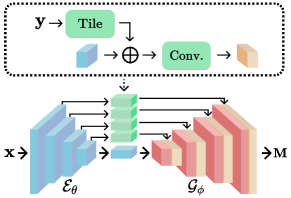
Figure 2: A detailed view of the Counterfactual Map Generator (CMG). A tiled one-hot target label $\mathbf{y}$ is concatenated to the skip connection. This enables the CMG to condition the counterfactual maps to be conditioned on an arbitrary target condition.

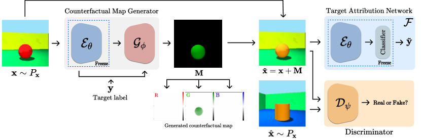
Figure 3: Schematic overview of Born Identity Network (BIN). There are two major components of BIN: Counterfactual Map Generator (CMG) and Target Attribution Network (TAN). The CMG synthesized a counterfactual map conditioned on arbitrary target label, while the TAN work towards enforcing target label attributes to the synthesized map.

3 Multi-way Counterfactual Map

Here, we formally define a multi-way counterfactual map. First, we define the dataset $P=(P_{\mathbf{x}},P_{\mathbf{y}})$, where $(\mathbf{x},\mathbf{y})\sim P_{\mathbf{x},\mathbf{y}}$ denote the data, label pair and $\mathbf{x}\sim P_{\mathbf{x}},\mathbf{y}\sim P_{\mathbf{y}}$ denote the unpaired data and label. We define a counterfactual map as a salient map that is able to produce a counterfactual explanation of a classifier $\mathcal{F}$. Formally, a single- or dual-way counterfactual map $\mathbf{M}_{\mathbf{x}}$ is a map that when added to an input sample $\mathbf{x}$, i.e., $\tilde{\mathbf{x}}=\mathbf{x}+\mathbf{M}_{\mathbf{x}}$, the classifier classifies it as another label complement to its original label, e.g., $\mathcal{F}(\mathbf{x})=true$ and $\mathcal{F}(\tilde{\mathbf{x}})=false$, and vice versa for dual-way counterfactual map. Here, if we are able to condition this counterfactual map with an attribute (or label), i.e., the multi-way counterfactual map $\mathbf{M}_{\mathbf{x},\mathbf{y}}$, we can transform an input sample as any other attribute of interest:

$$\tilde{\mathbf{x}}:=\mathbf{x}+\mathbf{M}_{\mathbf{x},\mathbf{y}}\quad\text{such that}\;\mathcal{F}(\tilde{\mathbf{x}})=\mathbf{y},$$ (1)

where data $\mathbf{x}$ and label $\mathbf{y}$ may be unpaired, i.e., we may condition the target label to be any one-hot vector (e.g., $\mathbf{y}$ can be a random one-hot vector or the posterior probability of the original input ($\mathbf{y}^{\prime}$ in Eq. 6)).

4 Born Identity Network

The goal of BIN is to induce counterfactual reasoning dependent on the target condition from a pre-trained model. To achieve this goal, we’ve devised BIN with two core modules, i.e., Counterfactual Map Generator (CMG) and Target Attribution Network (TAN), which work in a complementary manner in producing a multi-way counterfactual map. Specifically, the CMG synthesize conditioned maps, while the TAN enforces a target attribution to synthesized maps (Figure 3).

4.1 Counterfactual Map Generator

The CMG is a variant of Conditional GAN [27] that can synthesize a counterfactual map conditioned on a target label $\mathbf{y}$, i.e., $\mathbf{M}_{\mathbf{x},\mathbf{y}}$. Specifically, it consists of an encoder $\mathcal{E}_{\theta}$, a generator $\mathcal{G}_{\phi}$, and a discriminator $\mathcal{D}_{\psi}$. First, the network design of the encoder $\mathcal{E}_{\theta}$ and the generator $\mathcal{G}_{\phi}$ is a variation of U-Net [30] with a tiled target label concatenated to the skip connections (Figure 2). This generator design enables the generation to synthesize target conditioned maps such that multi-way counterfactual reasoning is possible. As a result, the counterfactual map is formulated as following:

$$\mathbf{M}_{\mathbf{x},\mathbf{y}}=\mathcal{G}_{\phi}\left(\mathcal{E}_{\theta}(\mathbf{x}),\mathbf{y}\right),$$ (2)

$$\tilde{\mathbf{x}}=\mathbf{x}+\mathbf{M}_{\mathbf{x},\mathbf{y}}.$$ (3)

Finally, following a general adversarial learning scheme, the discriminator discriminates real samples $\hat{\mathbf{x}}\sim P_{\mathbf{x}}$ from synthesized samples $\tilde{\mathbf{x}}$.

Counterfactual reasoning requires a good balance between the proposed hypothetical and given reality. In the following sections, we define the loss functions that guide the CMG to produce a well-balanced counterfactual map.

4.1.1 Adversarial Loss

For the adversarial loss functions, we have adopted the Least Square GAN (LSGAN) [26] objective function due to its stability during adversarial training. More specifically, LSGAN objective function contributes to a stable model training by penalizing samples far from the discriminator’s decision boundary. This objective function is an important choice for the BIN since the generated counterfactual maps should neither destroy the input appearance nor ignore the target attribution, i.e., it should contain a good balance between real and fake samples. To this end, the discriminator and the generator loss is defined as follows, respectively:

$$\begin{split}\mathcal{L}_{adv}^{\mathcal{D}_{\psi}}&=\frac{1}{2}\mathbb{E}_{\hat{\mathbf{x}}\sim P_{\mathbf{x}}}[(D_{\psi}(\hat{\mathbf{x}})-1)^{2}]\\ &+\frac{1}{2}\mathbb{E}_{\mathbf{x}\sim P_{\mathbf{x}},\mathbf{y}\sim P_{\mathbf{y}}}[(D_{\psi}(\tilde{\mathbf{x}}))^{2}],\end{split}$$ (4)

$$\mathcal{L}_{adv}^{\mathcal{G}_{\phi}} =\frac{1}{2}\mathbb{E}_{\mathbf{x}\sim P_{\mathbf{x}},\mathbf{y}\sim P_{\mathbf{y}}}[(D_{\psi}(\tilde{\mathbf{x}})-1)^{2}],$$ (5)

where $\mathbf{\tilde{x}}=\mathbf{x}+\mathbf{M}_{\mathbf{x},\mathbf{y}}$, $\mathbf{y}$ denote the random target label.

4.1.2 Cycle Consistency Loss

The cycle consistency loss is used for producing better multi-way counterfactual maps. In the scenario of an single-way counterfactual map generator, real samples $\hat{\mathbf{x}}$ and synthesized samples $\tilde{\mathbf{x}}$ are always sampled from one same specific class. This setting does not require a cycle consistency loss since the real and fake samples always have specified labels. However, since our discriminator only classifies the real or fake samples, it does not have the ability to guide the generator to produce multi-way counterfactual maps. Thus, we add a cycle consistency loss where the forward cycle produces a map with an arbitrary condition, i.e., $\mathbf{M}_{\mathbf{x},\mathbf{y}}$ generated from an unpaired data $\mathbf{x}\sim P_{\mathbf{X}}$ and random target label $\mathbf{y}\sim P_{\mathbf{y}}$, and the backward cycle produces a map conditioned on the posterior probability obtained from the classifier $\mathcal{F}$:

$$\begin{aligned} \mathcal{L}_{cyc}=\mathbb{E}_{\mathbf{x}\sim P_{\mathbf{x}},\mathbf{y}\sim P_{\mathbf{y}}}[\|(\tilde{\mathbf{x}}+\mathbf{M}_{\tilde{\mathbf{x}},\mathbf{y}^{\prime}})-\mathbf{x}\|_{1}],\end{aligned}$$ (6)

where $\mathbf{\tilde{x}}=\mathbf{x}+\mathbf{M}_{\mathbf{x},\mathbf{y}}$, $\mathbf{y}^{\prime}=\mathcal{F}(\mathbf{x})$, and $\mathbf{M}_{\tilde{\mathbf{x}},\mathbf{y}^{\prime}}=\mathcal{G}_{\phi}\left(\mathcal{E}_{\theta}(\tilde{\mathbf{x}}),\mathbf{y}^{\prime}\right)$.

4.2 Target Attribution Network

The TAN provides adequate assistance to the CMG by incorporating a target label to the synthesized conditioned map. Specifically, the objective of the TAN is to guide the generator to produce counterfactual maps that transform an input sample to be classified as a target class:

$$\mathcal{L}_{cls}=\mathbb{E}_{\mathbf{x}\sim P_{\mathbf{x}},\mathbf{y}\sim P_{\mathbf{y}}}[CE(\mathbf{y},\tilde{\mathbf{y}})],$$ (7)

where $\mathbf{y}$ denote the random target label, $\tilde{\mathbf{y}}=\mathcal{F}(\tilde{x})$, and $CE$ denote the cross-entropy function.

Conceptually, the role of the TAN is similar to that of a discriminator in GANs, but their objective is very different. While a discriminator learns to distinguish between real and fake samples, the TAN is already trained in classifying the input samples. Thus, the discriminator plays a min-max game with a generator in an effort to produce more realistic samples, while the TAN provides deterministic guidance for the generator to produce class-specific samples.

4.2.1 Counterfactual Map Loss

The counterfactual map loss limits the values of the counterfactual map to grow:

$$\mathcal{L}_{map}=\mathbb{E}_{\mathbf{x}\sim P_{\mathbf{x}},\mathbf{y}\sim P_{\mathbf{y}}}[\lambda_{1}\|\mathbf{M}_{\mathbf{x},\mathbf{y}}\|_{1}+\lambda_{2}\|\mathbf{M}_{\mathbf{x},\mathbf{y}}\|_{2}],$$ (8)

where $\lambda_{1}$ and $\lambda_{2}$ are weighting constants as the hyperparameter, and $\mathbf{y}$ is the random target label. This loss is crucial in solving two issues in counterfactual map generation. First, when left untethered, the counterfactual map will destroy the identity of the input sample. This problem is related to adversarial attacks [41], where a simple perturbation to the input sample will change the model’s decision. Second, from an end-user point of view, only the most important features should be represented as the counterfactual explanation. Thus, by placing a constraint on the magnitude of counterfactual maps, we can address the above issues in one step.

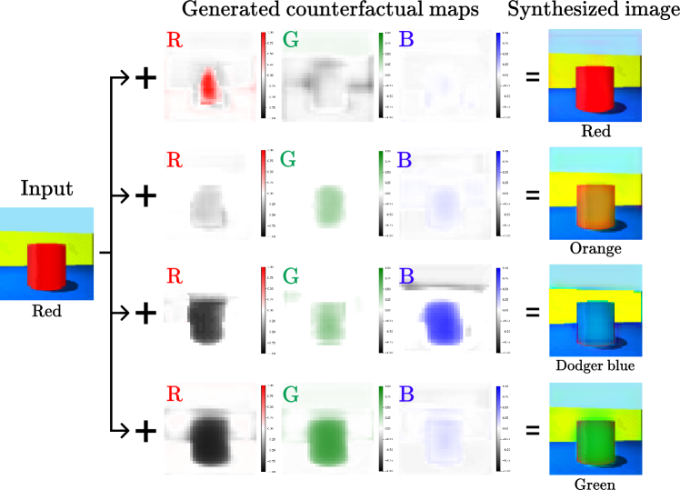
Figure 4: Examples of counterfactual maps for 3D Shapes [5] dataset. The counterfactual map consists of the RGB channel. This is the outcome of producing a counterfactual map where the red cylinder is classified as red, orange, dodger blue, and green hue cylinders.

4.3 Learning

Finally, we define the overall loss function for BIN as follows:

$$\mathcal{L}=\lambda_{3}\mathcal{L}^{\mathcal{D}_{\psi}}_{adv}+\lambda_{4}\mathcal{L}^{\mathcal{G}_{\phi}}_{adv}+\lambda_{5}\mathcal{L}_{cyc}+\lambda_{6}\mathcal{L}_{cls}+\mathcal{L}_{map},$$ (9)

where $\lambda$ is the hyperparameter of the model ($\lambda_{1}$ and $\lambda_{2}$ in Eq. 8).

During training, we share and fix the weights of the encoder $\mathcal{E}_{\theta}$ of the CMG with the TAN $\mathcal{F}$ to ensure that the attribution is consistent throughout the generative process. However, preliminary experiments on training the encoder $\mathcal{E}_{\theta}$ from scratch resulted in slightly lower qualitative and quantitative outcomes.

5 Experiments

We conduct various experiments to validate the counterfactual maps generated by our proposed method. First, we conducted a qualitative analysis of a multi-way counterfactual explanation. Second, we reported a quantitative analysis using a correlation measure between generated counterfactual maps and ground-truth maps. Finally, we performed a suite of ablation studies to verify that each component of the BIN towards creating a meaningful counterfactual map.

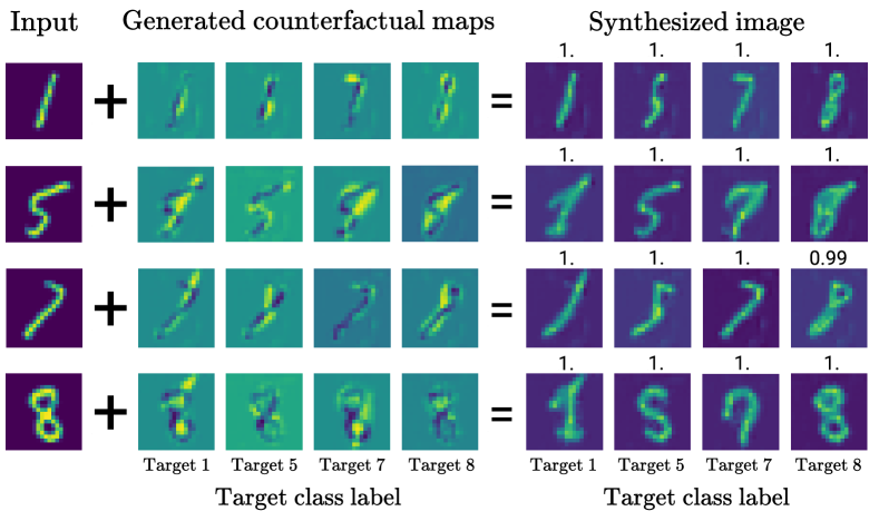
Figure 5: Examples of counterfactual maps for MNIST dataset. The resulting synthesized image is a addition between an input and its corresponding counterfactual map conditioned on a target label. The values on the top of each synthesized map is the model’s softmax activated logit.

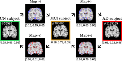
Figure 6: Examples of counterfactual maps for ADNI dataset (Subject ID 023_S_1190, Image ID on top left corner). Boundary boxes for green, orange, and red indicate ground-truths corresponding to CN, MCI, and AD, respectively, and the prediction scores at the bottom of each image are the model’s softmax activated logit.

5.1 Datasets

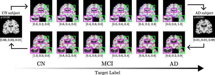
Figure 7: Example of counterfactual map conditioned on interpolated target labels (Subject ID 123_S_0106, Image ID on top left corner). The purple and green boxes correspond to the ventricular and cortex regions, respectively. The values at the bottom of left-most and right-most images are the model’s softmax activated logits, and the values at the bottom of top and bottom rows (i.e., interpolated images) are the target labels.

3D Shapes

The 3D Shapes dataset [5] consists of 480,000 RGB images of 3D geometric shapes with six latent factors (10 floors/wall/object hues, 8 scales, 4 shapes, and 15 orientations). For our experiments, we selected red, orange, dodger blue, and green object hues as the target classes. We randomly divided the dataset into a train, validation, and test set at a ratio of 8:1:1 and applied channel-wise min-max normalization.

MNIST

For MNIST dataset, we used the data split provided by [24] and applied min-max normalization.

ADNI

ADNI dataset [29] consists of 3D Magnetic Resonance Imaging (MRI) of various subject groups ranging from Cognitive Normal (CN) to Alzheimer’s Disease (AD). For this dataset, we have selected a baseline MRI of 433 CN subjects, 748 Mild Cognitive Impairment (MCI) subjects, and 359 AD subjects in ADNI 1/2/3/Go studies. MCI is considered as a prodromal stage (i.e., preceding stage) of AD [34], which is a transitional state between normal cognitive changes and early clinical symptoms of dementia.

For longitudinal studies, we have selected 12 CN test subjects that have converted to the AD group after the MCI stage at any given time. With the exception of 12 longitudinal test subjects, all subjects were randomly split into train, validation, and test sets at a ratio of 8:1:1. The pre-processing procedure consisted of neck removal (FSL v6.0.1 robustfov), brain extraction (HDBet [21]), linear registration (FSL v6.0.1 FLIRT), zero-mean unit-variance normalization, quantile normalization at 10% and 90%, and down-scaling by $2\times$. The resulting pre-processed MRI is a $96\times 114\times 96$ image. We used default parameters from FSL v6.0.1 [22].

5.2 Implementation

For 3D Shapes and MNIST experiments, we re-implemented the model from Kim et al. [23] with minor modifications. SonoNet-16 [3] is used for ADNI dataset as the encoder $\mathcal{E}_{\theta}$. The generator $\mathcal{G}_{\phi}$ has the same network design as the encoder $\mathcal{E}_{\theta}$ with pooling layers replaced by up-sampling layers. The test accuracy of the pre-trained TAN $\mathcal{F}$ is 99.56% for MNIST, 99.81% for 3D Shapes, and 73.79% for ADNI dataset, respectively. For compared methods, i.e., attribution-based approaches (Integrated gradients [38], LRP-Z [1], DeepLift [33]) and perturbation-based approach (Guided backpropagation [32]), we used the pre-trained TAN $\mathcal{F}$ as the classifier. Further implementation details are in the Supplementary.

5.3 Qualitative Analysis

An N-way counterfactual map is a map that when added to an input sample, the classifier classifies it as a targeted class. The N-way term refers to the degree of freedom of the targeted class. In the following sections, we compared and validated multi-way counterfactual maps in various settings. Specifically, we took a bottom-up analysis approach with experiments on a toy example building up to application in a real-world dataset. First, we analyzed our novel multi-way counterfactual maps using an easy-to-understand toy example, which is the 3D Shapes and MNIST dataset. Additionally, we applied our proposed BIN in a real-world dataset and compared it with state-of-the-art XAI frameworks with ADNI dataset.

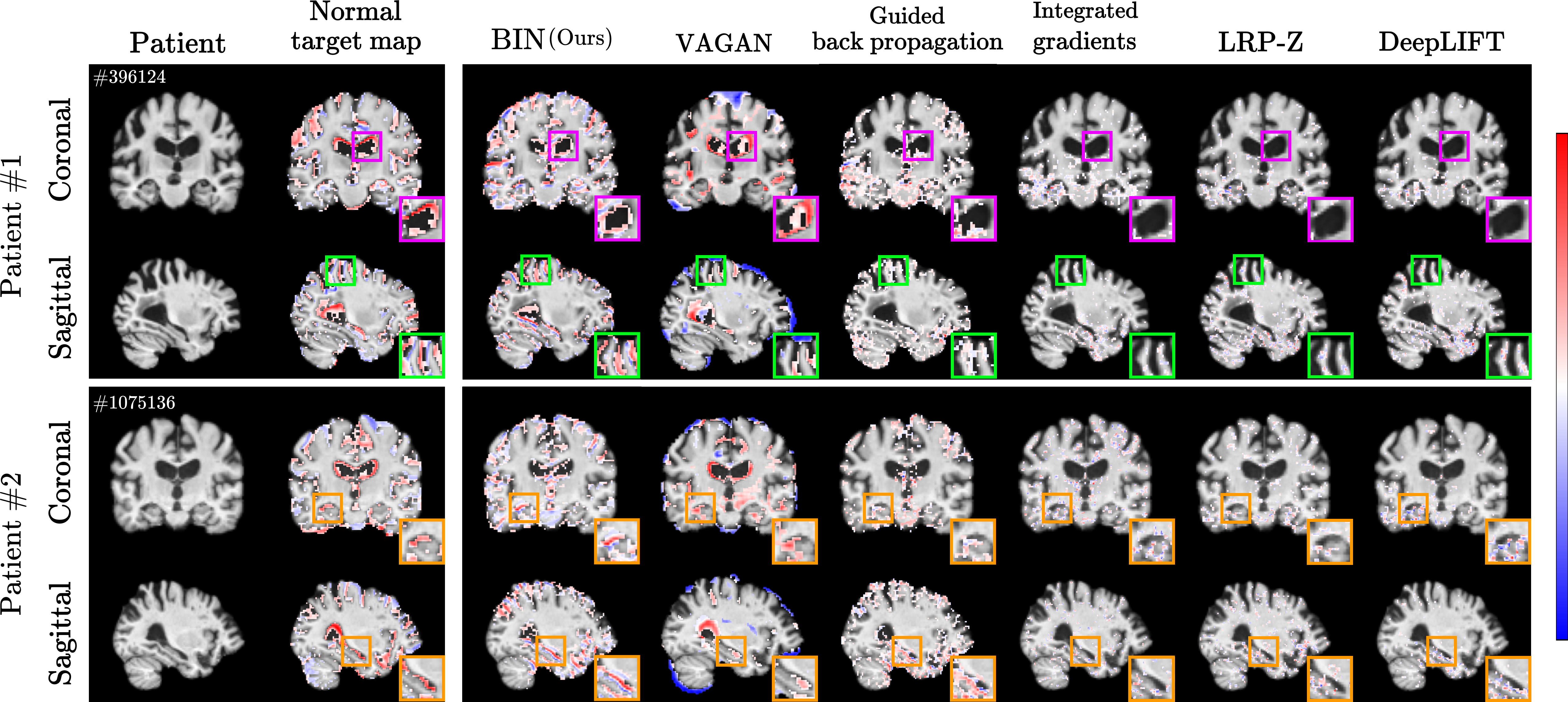
Figure 8: Example of counterfactual maps for ADNI dataset (Patient #1 ID 024_S_0985, patient #2 ID 002_S_4225, Image ID on top left corner). Purple, green, orange boxes visualize ventricular, cortex, and hippocampal regions, respectively.

5.3.1 Validation of Counterfactual Map

3D Shapes

We analyzed multi-way counterfactual maps using 3D Shapes dataset (Figure 4). The goal of this experiment is to verify that our counterfactual map is able to transform an input image with regard to a target latent factor, i.e., object hue. The first row shows the counterfactual map from red (R: 255, G: 0, B: 0) to red (R: 255, G: 0, B: 0), i.e., for transforming to its own hue. Although an ideal counterfactual map (i.e., zero-value map) was not generated, each color channel of the map is a minor variation that does not destroy the input’s hue. The third and fourth row transformed red (R:255, G: 0, B: 0) to dodger blue (R: 30, G: 144, B: 255) and green (R: 0, G: 255, B: 0), respectively. Despite the contrasting hue in all channels, the BIN was able to induce the counterfactual map corresponding to the target object hue. In addition, the classification performance on the synthesized image is 99.12%, indicating that the counterfactual map has successfully transformed the input image to be classified as another label. Furthermore, we have performed an interpolation, and this result is included in the Supplementary.

Invariance of Irrelevant Factors

In most counterfactual maps generated in this experiment, we have observed an interesting phenomenon in which the counterfactual maps are relatively invariant to latent factors that were not targeted for transformation. For example, the scale and shape of the object in the counterfactual map are relatively similar to that of the input image. This indicates that our counterfactual map is somewhat localized to the target latent factor.

MNIST

We generated multi-way counterfactual maps for MNIST dataset (Figure 5). In plain sight, we can observe that the style of an input image is maintained. This was related to the invariant to non-targeted latent factors observed in 3D Shapes experiment. We hypothesize that this invariant is due to the counterfactual map loss (Eq. (8)) since it puts constraints on the values of the counterfactual map so that it transforms an input sample with the least amount of energy. From a conceptual view, our generated counterfactual map exhibited a good example of counterfactual reasoning since it can successfully produce hypothetical realities with regards to a given input sample.

5.3.2 Application in Medical Domain

To validate that our BIN can be generalized in the medical domain, we investigated multi-way counterfactual maps using ADNI dataset (Figure 6), which possesses suitable scenarios in terms of its progression stage.

Multi-way Counterfactual Map Interpolation

One of the biomarkers of Alzheimer’s disease is an atrophy in brain regions, such as the ventricular [10], cortical thickness [7, 12], and hippocampus [20, 25, 14]. As observed in the multi-way counterfactual maps (Figure 7), atrophy is clearly visible in those regions.

Normal Target Map

Since there are no ground-truth maps for ADNI dataset, we utilized the Normal target map from longitudinal test subjects (second column in Figure 8). First, we have gathered MRIs from 12 subjects who converted from CN (baseline) to MCI and AD at any given time (subject ID in the Supplementary). Then, to create the Normal target map, we subtracted the baseline image from the target class image. This Normal target map exhibited a good representation of a ground-truth map of disease localization since we can observe which regions are possibly responsible for the conversion. The counterfactual map generated by attribution-based approaches (Integrated gradients, LRP-Z, DeepLift) and perturbation-based approach (Guided backpropagation) does not clearly showed the regions responsible for.

Table 1: Normalized Cross-Correlation (NCC) scores for 3D Shapes and ADNI dataset².

Method	3D Shapes		ADNI
	NCC(+)	NCC(-)	NCC(+)	NCC(-)
LRP-Z [1]	0.008	0.086	0.008	0.005
Integrated Gradients [38]	0.006	0.152	0.006	0.005
DeepLIFT [33]	0.007	0.183	0.005	0.004
Guided Backprop [32]	0.183	0.123	0.239	0.204
VAGAN [4]	0.381	-	0.317	-
BIN (ours)	0.537	0.452	0.364	0.201

5.4 Quantitative Analysis

In this section, we quantitatively evaluated our proposed BIN and compared it with the outcome of other methods. To quantitatively assess the quality of our generated counterfactual maps, we’ve calculated the Normalized Cross-Correlation (NCC) score between generated maps and ground-truth maps. NCC score measures the similarity between two samples in a normalized setting, i.e., Higher NCC scores denote higher similarity. Thus, NCC can be helpful when two samples have a different magnitude of signals. However, since MNIST dataset does not have ground-truth maps, we have performed a different quantitative evaluation in section 5.5. For the ADNI dataset, we used the Normal target map described in section 5.3.2 as the ground-truth map. Detailed results for all multi-way cases (e.g., transform AD to MCI or CN to AD, etc.) are in the Supplementary.

5.5 Ablation Studies

We conducted a suite of ablation studies to assess each component of the BIN in creating a counterfactual map. Specifically, we focused on ablation studies on the conditioned generator (denoted as $\mathbf{y}$), the Target Attribution Network loss ($\mathcal{L}_{cls}$), cycle consistency loss ($\mathcal{L}_{cyc}$), and the Counterfactual Map loss ($\mathcal{L}_{map}$).

Normalized Cross Correlation

For the ADNI and 3D Shapes dataset, we calculated NCC scores with the same settings as section 5.4 (Table  2). The reported scores indicate every component of the BIN was crucial for producing a meaningful counterfactual map. However, ablating the TAN loss $\mathcal{L}_{cls}$ showed a significant drop in NCC scores, indicating that it is one of the most crucial components of the BIN. The TAN guided the generative process to build targeted class attribution, which works in a similar manner to a discriminator in GANs. The cycle consistency loss $\mathcal{L}_{cyc}$ ensured the counterfactual map to contain information on its identity, i.e., input sample. In a preliminary experiment, we have observed that cycle consistency loss helps generate more crisp counterfactual maps, indicating that it works as a regularizer for the BIN. The counterfactual map loss $\mathcal{L}_{map}$ was another important component of the BIN since it regulates which region is most important.

Table 2: Normalized Cross-Correlation (NCC) scores for ablation studies.

Removed	3D Shapes		ADNI
Components	NCC(+)	NCC(-)	NCC(+)	NCC(-)
$\mathbf{y}$	0.290	0.225	0.234	0.112
$\mathcal{L}_{cls}$	0.213	0.145	0.066	0.073
$\mathcal{L}_{cyc}$	0.501	0.362	0.279	0.145
$\mathcal{L}_{map}$	0.311	0.212	0.267	0.160
$\mathcal{L}_{cls},\mathcal{L}_{map}$	0.096	0.088	0.072	0.080
All above	0.029	0.070	0.062	0.051
BIN (ours)	0.537	0.452	0.364	0.201

Fréchet Inception Distance

For a quantitative assessment of multi-way counterfactual map, we used a Fréchet Inception Distance [18] commonly used for assessing the generative performance of GANs. Here, we’ve selected 4,000 test samples for counterfactual map generation (i.e. fake images), and 4,000 test samples as real images. Since a counterfactual map can transform any number to any other number, a single image can generate 10 images (one per number). Thus, the total number of fake samples we’ve generated is 40,000 (i.e., 4,000 fake images per number). We compared our work in an ablation study setting (table in the Supplementary). In most of the settings, our proposed BIN performed significantly better.

6 Discussion

For most experiments, reported NCC(-) scores for almost every compared method were lower than that of NCC(+). A possible explanation is that the activation functions, such as ReLU, may be imposing a positive bias or negative skewness on the model output. For example, the mean and mode of a counterfactual map for almost every datasets and every method compared in this paper were slightly over zero. This may result in imposing a constraint for subtraction operations which lowers the NCC(-) scores. Possible future work for the community is to verify whether this bias or skewness really exists and propose a way to alleviate this.

7 Conclusion

In this work, we proposed Born Identity Network (BIN), which is a post-hoc approach for producing multi-way counterfactual maps in multiple hypothetical scenarios. By visualizing counterfactual explanations at the level of human knowledge through our BIN, classifiers that have derived high performance in various domains can provide explainability and interpretability of higher quality. It is expected that BIN will be a practical application that helps diagnose or predict disease through a counterfactual visual explanation of its applicability in the multi-classifier dealing with the medical field.

Supplementary

Section 1: Extra Counterfactual Map Interpolation

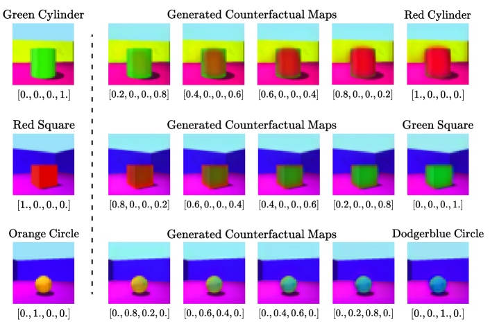
Figure S1: Example of counterfactual map for 3D Shapes dataset conditioned on interpolated target labels. The one-hot vector at the bottom of each counterfactual map is the target labels.

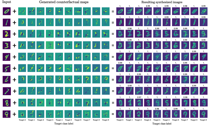
Figure S2: Examples of counterfactual maps for MNIST dataset. The resulting synthesized image is an addition between an input and its corresponding counterfactual map conditioned on a target label. The values on the top of each confound map are the model’s softmax activated logit.

Section 2: NCC Scores in Multi-way Settings

For an in-depth analysis of the our multi-way counterfactual maps, we calculated NCC(+) and NCC(-) scores in a multi-class setting (i.e., AD $\leftrightarrow$ CN, AD $\leftrightarrow$ MCI, and MCI $\leftrightarrow$ CN). With the exception of VAGAN, all methods utilize the same 3-class (CN vs. MCI vs. AD) classifier. Note that VAGAN is a single-way method with the assumption that the label of observation is known. In other words, it is not possible to obtain scores of NCC(+) and NCC(-) simultaneously from a single model. The results of VAGAN in Table S1 are from six different models, while all other methods are from the same classifier.

Table S1: Normalized Cross-Correlation (NCC) scores for all multi-way cases in ADNI dataset.

Method	AD $\leftrightarrow$ CN		AD $\leftrightarrow$ MCI		MCI $\leftrightarrow$ CN
	NCC(+)	NCC(-)	NCC(+)	NCC(-)	NCC(+)	NCC(-)
LRP-Z [1]	0.008	0.005	0.006	0.004	0.005	0.005
Integrated Gradients [38]	0.006	0.005	0.007	0.007	0.006	0.007
DeepLIFT [33]	0.005	0.004	0.006	0.004	0.004	0.005
Guided Backprop [32]	0.239	0.204	0.212	0.163	0.199	0.158
VAGAN [4]	0.317	0.298	0.285	0.257	0.283	0.186
BIN (ours)	0.364	0.201	0.301	0.174	0.292	0.188

Section 3: Ablation Studies - Fréchet Inception Distance

Since there are no ground truth counterfactual maps (i.e., Normal target maps) for MNIST dataset, we calculated the Fréchet Inception Distance [18] score, which is commonly used to assess the synthesized images of generative models. In addition, we performed a suite of ablations studies on core components of BIN.

Table S2: Fréchet Inception Distance (FID) scores reported for ablation studies for MNIST dataset.

Components				FID score
$\mathbf{y}$	$\mathcal{L}_{cls}$	$\mathcal{L}_{cyc}$	$\mathcal{L}_{map}$	0	1	2	3	4	5	6	7	8	9	avg
	✓	✓	✓	1.340	1.082	1.034	0.935	0.945	0.933	0.999	0.850	0.961	0.850	0.993
✓		✓	✓	1.338	1.241	1.039	0.955	1.064	0.973	1.022	0.956	0.993	0.935	1.052
✓	✓		✓	1.283	1.156	0.915	0.810	0.959	0.822	0.987	0.888	0.896	0.834	0.955
✓	✓	✓		1.318	1.056	0.906	0.804	0.951	0.824	1.001	0.841	0.904	0.841	0.945
✓			✓	1.338	1.242	1.039	0.956	1.065	0.973	1.022	0.956	0.993	0.935	1.052
				1.338	1.242	1.039	0.956	1.065	0.973	1.022	0.956	0.993	0.935	1.052
✓	✓	✓	✓	1.211	0.902	0.892	0.802	0.958	0.812	0.970	0.835	0.912	0.833	0.912

Section 4: Preliminary Survey on Related Works

Table S3: Preliminary Survey on Related Works

	Method	Way	Stratification	Counterfactual Map	Post-hoc
Sauer $\emph{et al}.$ [31]	Generative	Single	$\times$	$\surd$	$\surd$
Goyal $\emph{et al}.$ [17]	Perturbation	Dual	$\times$	$\times$	$\surd$
Baumgartner $\emph{et al}.$ [4]	Generative	Single	$\times$	$\surd$	$\times$
Chang $\emph{et al}.$ [6]	Perturbation	Single	$\times$	$\times$	$\surd$
Singla $\emph{et al}.$ [36]	Generative	Dual	$\surd$	$\times$	$\surd$
Bass $\emph{et al}.$ [2]	Generative	Dual	$\surd$	$\surd$	$\times$
Ours	Generative	Multi	$\surd$	$\surd$	$\surd$

The generation-based method is an interpretation model that uses a generative process to produce visual explanations. There are roughly two different manners in which generative models approach visual explanations: generative explanation, and counterfactual explanation. Generative explanation ($\emph{i.e}.\hbox{},$ generating $\tilde{\mathbf{x}}$) approach that focuses on generating images to be classified as a target class, rather than conducting analytic reasoning. Counterfactual explanation approach ($\emph{i.e}.\hbox{},$ generating $\mathbf{M}$, where $\tilde{\mathbf{x}}=\mathbf{x}+\mathbf{M}$) questions what and why a sample was classified as a target class, which can be intuitively inferred through the generated counterfactual map.

Most works on counterfactual maps exploit single- or dual-way explanation, which can only provide one or two hypothetical alternatives for counterfactual reasoning. Stratification, in the context of counterfactual reasoning, provides explanation in a continuous space. This allows counterfactual maps to be generated for any point between two or more outcomes (e.g., normal and Alzheimer’s disease), where without it, counterfactual maps can only explain extreme tails of the outcome. However, stratified single-/dual-way counterfactual maps cannot model the complex and non-linear progression from one outcome (e.g., normal) to other (e.g., Alzheimer’s disease). Thus, they are only able to draw a linear interpolation between the two outcomes. When stratification is combined with multi-way counterfactual maps, these generated maps can model a more precise and realistic progression from one outcome to the other. Thus, multi-way stratified counterfactual maps allow explanation for predefined multiple outcomes, as well as interpolate to undefined outcomes.

Non-post-hoc methods build interpretable models or modules from scratch, while post-hoc methods builds on top of a pretrained model. Thus, post-hoc methods are a more generalized interpretation method that can be applied to most connectionist models.

Section 5: Details of Longitudinal Dataset

Since there are no ground-truth maps for ADNI dataset [29], we utilized the Normal target map from longitudinal test subjects. First, we have gathered MRIs from 12 subjects who converted from CN (baseline) to MCI and AD at any given time. Then, to create the Normal target map, we subtracted the baseline image from the target class image. This Normal target map exhibited a good representation of a ground-truth map of disease localization since we can observe which regions are possibly responsible for the conversion.

We have selected 12 CN test subjects that have converted to the AD group after the MCI stage at any given time. Details of the subject ID with regard to each subject and image ID corresponding to CN, MCI, and AD are shown in the Table S4.

Table S4: ADNI longitudinal subject information for the quantitative evaluation of counterfactual map

Subject ID	Cognitive Normal	Mild Cognitive Impairment	Alzheimer’s Disease
	Image ID	Image ID	Image ID
$023\_\text{S}\_0061$	9046	401795	473765
$123\_\text{S}\_0106$	10126	213947	865961
$131\_\text{S}\_0123$	10042	292389	475755
$005\_\text{S}\_0223$	11645	26115	143296
$037\_\text{S}\_0467$	14861	169074	372375
$129\_\text{S}\_0778$	20543	205611	388698
$024\_\text{S}\_0985$	27607	342890	396124
$023\_\text{S}\_1190$	35585	780686	1135165
$002\_\text{S}\_4262$	259653	397601	788894
$029\_\text{S}\_4385$	285589	421501	642470
$098\_\text{S}\_4506$	286987	714545	1073489
$051\_\text{S}\_5285$	396288	1055626	1182436

Section 6: Network Architecture

$(\cdot)^{*}$ denotes the skip-connection layer that passed through the convolution layer of 3 kernel size, 1 stride after concatenation with the tiled target label. In the case of feature maps used in $(\cdot)^{*}$, we used the same number of feature maps of the counterfactual map generator to be concatenated.

We performed $n$-D convolutional operation in the order of Conv.$\rightarrow$BatchNorm./SpectralNorm.$\rightarrow$Activation. For the 3D Shapes and MNIST experiments, we re-implemented the encoder $\mathcal{E}_{\theta}$ from Kim et al. [23] with minor modification. In ADNI experiment, the encoder $\mathcal{E}_{\theta}$ network of SonoNet-16 [3] was used identically.

6-1. 3D Shapes

Table S5: 3D Shapes encoder $\mathcal{E}_{\theta}$ network.

Operation	Feature Maps	Batch Norm.	Kernels	Strides	Padding	Activation
Input $\mathbf{x}\in\mathbb{R}^{64\times 64\times 3}$
(ENC1) 2D Conv.	32	$\surd$	(4 $\times$ 4)	(2 $\times$ 2)	$\surd$	ReLU
(ENC2) 2D Conv.	32	$\surd$	(4 $\times$ 4)	(2 $\times$ 2)	$\surd$	ReLU
(ENC3) 2D Conv.	64	$\surd$	(4 $\times$ 4)	(2 $\times$ 2)	$\surd$	ReLU
(ENC4) 2D Conv.	64	$\surd$	(4 $\times$ 4)	(2 $\times$ 2)	$\surd$	ReLU
Output $\mathbf{z}\in\mathbb{R}^{4\times 4\times 64}$

Table S6: 3D Shapes classifier $\mathcal{F}$ network.

Operation	Feature Maps	Batch Norm.	Dropout	Activation
Input $\mathbf{z}\in\mathbb{R}^{4\times 4\times 64}$
Fully Connected	4	$\times$	$\times$	Softmax

Table S7: 3D Shapes discriminator $\mathcal{D}_{\psi}$ network.

Operation	Feature Maps	Spectral Norm.	Kernels	Strides	Padding	Activation
Input $\mathbf{x}\in\mathbb{R}^{64\times 64\times 3}$
2D Conv.	32	$\times$	(4 $\times$ 4)	(2 $\times$ 2)	$\surd$	Leaky ReLU
2D Conv.	32	$\surd$	(4 $\times$ 4)	(2 $\times$ 2)	$\surd$	Leaky ReLU
2D Conv.	64	$\surd$	(4 $\times$ 4)	(2 $\times$ 2)	$\surd$	Leaky ReLU
2D Conv.	64	$\surd$	(4 $\times$ 4)	(2 $\times$ 2)	$\surd$	Leaky ReLU
Fully Connected	1	$\times$				Linear

Table S8: 3D Shapes counterfactual map generator $\mathcal{G}_{\phi}$ network.

Operation	Feature Maps	Batch Norm.	Kernels	Strides	Padding	Activation
Input $\mathbf{z}\in\mathbb{R}^{4\times 4\times 64}$
(DEC3) Upsampling				(2 $\times$ 2)
Concatenate $\text{(ENC3)}^{*}$ and (DEC3) along the channel axis
2D Conv.	64	$\surd$	(3 $\times$ 3)	(1 $\times$ 1)	$\surd$	ReLU
(DEC2) Upsampling				(2 $\times$ 2)
Concatenate $\text{(ENC2)}^{*}$ and (DEC2) along the channel axis
2D Conv.	32	$\surd$	(3 $\times$ 3)	(1 $\times$ 1)	$\surd$	ReLU
(DEC1) Upsampling				(2 $\times$ 2)
Concatenate $\text{(ENC1)}^{*}$ and (DEC1) along the channel axis
2D Conv.	32	$\surd$	(3 $\times$ 3)	(1 $\times$ 1)	$\surd$	ReLU
Upsampling				(2 $\times$ 2)
2D Conv.	3	$\surd$	(1 $\times$ 1)	(1 $\times$ 1)	$\surd$	Tanh

6-2. MNIST

Table S9: MNIST encoder $\mathcal{E}_{\theta}$ network.

Operation	Feature Maps	Batch Norm.	Kernels	Strides	Padding	Activation
Input $\mathbf{x}\in\mathbb{R}^{28\times 28\times 1}$
2D Conv.	32	$\surd$	(3 $\times$ 3)	(1 $\times$ 1)	$\surd$	ReLU
(ENC1) 2D Conv.	32	$\surd$	(4 $\times$ 4)	(2 $\times$ 2)	$\surd$	ReLU
2D Conv.	64	$\surd$	(3 $\times$ 3)	(1 $\times$ 1)	$\surd$	ReLU
(ENC2) 2D Conv.	64	$\surd$	(4 $\times$ 4)	(2 $\times$ 2)	$\surd$	ReLU
2D Conv.	128	$\surd$	(3 $\times$ 3)	(1 $\times$ 1)	$\surd$	ReLU
(ENC3) 2D Conv.	128	$\surd$	(4 $\times$ 4)	(2 $\times$ 2)	$\surd$	ReLU
2D Conv.	256	$\surd$	(3 $\times$ 3)	(1 $\times$ 1)	$\surd$	ReLU
(ENC4) 2D Conv.	256	$\surd$	(4 $\times$ 4)	(2 $\times$ 2)	$\surd$	ReLU
Output $\mathbf{z}\in\mathbb{R}^{2\times 2\times 256}$

Table S10: MNIST classifier $\mathcal{F}$ network.

Operation	Feature Maps	Batch Norm.	Dropout	Activation
Input $\mathbf{z}\in\mathbb{R}^{2\times 2\times 256}$
Fully Connected	128	$\times$	0.5	ReLU
Fully Connected	10	$\times$	0.25	Softmax

Table S11: MNIST discriminator $\mathcal{D}_{\psi}$ network.

Operation	Feature Maps	Batch Norm.	Kernels	Strides	Padding	Activation
Input $\mathbf{x}\in\mathbb{R}^{28\times 28\times 1}$
2D Conv.	32	$\times$	(3 $\times$ 3)	(1 $\times$ 1)	$\surd$	Leaky ReLU
2D Conv.	32	$\surd$	(4 $\times$ 4)	(2 $\times$ 2)	$\surd$	Leaky ReLU
2D Conv.	64	$\surd$	(3 $\times$ 3)	(1 $\times$ 1)	$\surd$	Leaky ReLU
2D Conv.	64	$\surd$	(4 $\times$ 4)	(2 $\times$ 2)	$\surd$	Leaky ReLU
2D Conv.	128	$\surd$	(3 $\times$ 3)	(1 $\times$ 1)	$\surd$	Leaky ReLU
2D Conv.	128	$\surd$	(4 $\times$ 4)	(2 $\times$ 2)	$\surd$	Leaky ReLU
2D Conv.	256	$\surd$	(3 $\times$ 3)	(1 $\times$ 1)	$\surd$	Leaky ReLU
2D Conv.	256	$\surd$	(4 $\times$ 4)	(2 $\times$ 2)	$\surd$	Leaky ReLU
Fully Connected	1	$\times$				Linear

Table S12: MNIST counterfactual map generator $\mathcal{G}_{\phi}$ network.

Operation	Feature Maps	Batch Norm.	Kernels	Strides	Padding	Activation
Input $\mathbf{z}\in\mathbb{R}^{2\times 2\times 256}$
Upsampling				(2 $\times$ 2)
(DEC3) 2D Conv.	128	$\surd$	(3 $\times$ 3)	(1 $\times$ 1)	$\surd$	ReLU
Concatenate $\text{(ENC3)}^{*}$ and (DEC3) along the channel axis
2D Conv.	128	$\surd$	(3 $\times$ 3)	(1 $\times$ 1)	$\surd$	ReLU
Upsampling				(2 $\times$ 2)
(DEC2) 2D Conv.	64	$\surd$	(2 $\times$ 2)	(1 $\times$ 1)		ReLU
Concatenate $\text{(ENC2)}^{*}$ and (DEC2) along the channel axis
2D Conv.	64	$\surd$	(3 $\times$ 3)	(1 $\times$ 1)	$\surd$	ReLU
Upsampling				(2 $\times$ 2)
(DEC1) 2D Conv.	32	$\surd$	(3 $\times$ 3)	(1 $\times$ 1)	$\surd$	ReLU
Concatenate $\text{(ENC1)}^{*}$ and (DEC1) along the channel axis
2D Conv.	32	$\surd$	(3 $\times$ 3)	(1 $\times$ 1)	$\surd$	ReLU
2D Deconv.	1	$\surd$	(4 $\times$ 4)	(2 $\times$ 2)	$\surd$	Tanh

6-3. ADNI

Table S13: ADNI encoder $\mathcal{E}_{\theta}$ network.

Operation	Feature Maps	Batch Norm.	Kernels	Strides	Padding	Activation
Input $\mathbf{x}\in\mathbb{R}^{96\times 114\times 96\times 1}$
3D Conv.	16	$\surd$	(3 $\times$ 3 $\times$ 3)	(1 $\times$ 1 $\times$ 1)	$\surd$	ReLU
(ENC1) 3D Conv.	16	$\surd$	(3 $\times$ 3 $\times$ 3)	(1 $\times$ 1 $\times$ 1)	$\surd$	ReLU
Max Pooling			(2 $\times$ 2 $\times$ 2)	(2 $\times$ 2 $\times$ 2 )
3D Conv.	32	$\surd$	(3 $\times$ 3 $\times$ 3)	(1 $\times$ 1 $\times$ 1)	$\surd$	ReLU
(ENC2) 3D Conv.	32	$\surd$	(3 $\times$ 3 $\times$ 3)	(1 $\times$ 1 $\times$ 1)	$\surd$	ReLU
Max Pooling			(2 $\times$ 2 $\times$ 2)	(2 $\times$ 2 $\times$ 2)
3D Conv.	64	$\surd$	(3 $\times$ 3 $\times$ 3)	(1 $\times$ 1 $\times$ 1)	$\surd$	ReLU
3D Conv.	64	$\surd$	(3 $\times$ 3 $\times$ 3)	(1 $\times$ 1 $\times$ 1)	$\surd$	ReLU
(ENC3) 3D Conv.	64	$\surd$	(3 $\times$ 3 $\times$ 3)	(1 $\times$ 1 $\times$ 1)	$\surd$	ReLU
Max Pooling			(2 $\times$ 2 $\times$ 2)	(2 $\times$ 2 $\times$ 2)
3D Conv.	128	$\surd$	(3 $\times$ 3 $\times$ 3)	(1 $\times$ 1 $\times$ 1)	$\surd$	ReLU
3D Conv.	128	$\surd$	(3 $\times$ 3 $\times$ 3)	(1 $\times$ 1 $\times$ 1)	$\surd$	ReLU
(ENC4) 3D Conv.	128	$\surd$	(3 $\times$ 3$\times$ 3)	(1 $\times$ 1 $\times$ 1)	$\surd$	ReLU
Max Pooling			(2 $\times$ 2 $\times$ 2)	(2 $\times$ 2 $\times$ 2)
3D Conv.	128	$\surd$	(3 $\times$ 3 $\times$ 3)	(1 $\times$ 1 $\times$ 1)	$\surd$	ReLU
3D Conv.	128	$\surd$	(3 $\times$ 3 $\times$ 3)	(1 $\times$ 1 $\times$ 1)	$\surd$	ReLU
3D Conv.	128	$\surd$	(3 $\times$ 3 $\times$ 3)	(1 $\times$ 1 $\times$ 1)	$\surd$	ReLU
Output $\mathbf{z}\in\mathbb{R}^{6\times 7\times 6\times 128}$

Table S14: ADNI classifier $\mathcal{F}$ network.

Operation	Feature Maps	Batch Norm.	Dropout	Activation
Input $\mathbf{z}\in\mathbb{R}^{6\times 7\times 6\times 128}$
Fully Connected	256	$\times$	$\times$	ReLU
Fully Connected	3	$\times$	$\times$	Softmax

Table S15: ADNI discriminator $\mathcal{D}_{\psi}$ network.

Operation	Feature Maps	Batch Norm.	Kernels	Strides	Padding	Activation
Input $\mathbf{x}\in\mathbb{R}^{96\times 114\times 96\times 1}$
3D Conv.	16	$\times$	(3 $\times$ 3 $\times$ 3)	(1 $\times$ 1 $\times$ 1)	$\surd$	Leaky ReLU
3D Conv.	16	$\surd$	(4 $\times$ 4 $\times$ 4)	(1 $\times$ 2$\times$ 2)	$\surd$	Leaky ReLU
3D Conv.	32	$\surd$	(3 $\times$ 3 $\times$ 3)	(1 $\times$ 1 $\times$ 1)	$\surd$	Leaky ReLU
3D Conv.	32	$\surd$	(4 $\times$ 4 $\times$ 4)	(1 $\times$ 2 $\times$ 2)	$\surd$	Leaky ReLU
3D Conv.	64	$\surd$	(3 $\times$ 3 $\times$ 3)	(1 $\times$ 1 $\times$ 1)	$\surd$	Leaky ReLU
3D Conv.	64	$\surd$	(3 $\times$ 3 $\times$ 3)	(1 $\times$ 1 $\times$ 1)	$\surd$	Leaky ReLU
3D Conv.	64	$\surd$	(4 $\times$ 4 $\times$ 4)	(2 $\times$ 2 $\times$ 2)	$\surd$	Leaky ReLU
3D Conv.	128	$\surd$	(3 $\times$ 3 $\times$ 3)	(1 $\times$ 1 $\times$ 1)	$\surd$	Leaky ReLU
3D Conv.	128	$\surd$	(3 $\times$ 3 $\times$ 3)	(1 $\times$ 1 $\times$ 1)	$\surd$	Leaky ReLU
3D Conv.	128	$\surd$	(4 $\times$ 4 $\times$ 4)	(2 $\times$ 2 $\times$ 2)	$\surd$	Leaky ReLU
3D Conv.	256	$\surd$	(3 $\times$ 3 $\times$ 3)	(1 $\times$ 1 $\times$ 1)	$\surd$	Leaky ReLU
3D Conv.	256	$\surd$	(3 $\times$ 3 $\times$ 3)	(1 $\times$ 1 $\times$ 1)	$\surd$	Leaky ReLU
3D Conv.	256	$\surd$	(4 $\times$ 4 $\times$ 4)	(2 $\times$ 2 $\times$ 2)	$\surd$	Leaky ReLU
3D Conv.	64	$\surd$	(1 $\times$ 1 $\times$ 1)	(1 $\times$ 1 $\times$ 1)	$\surd$	Leaky ReLU
3D Conv.	1	$\surd$	(1 $\times$ 1 $\times$ 1)	(1 $\times$ 1 $\times$ 1)	$\surd$	Linear
Global Average Pooling

Table S16: ADNI counterfactual map generator $\mathcal{G}_{\phi}$ network.

Operation	Feature Maps	Batch Norm.	Kernels	Strides	Padding	Activation
Input $\mathbf{z}\in\mathbb{R}^{6\times 7\times 6\times 128}$
(DEC4) Upsampling				(2 $\times$ 2 $\times$ 2)
Concatenate $\text{(ENC4)}^{*}$ and (DEC4) along the channel axis
3D Conv.	128	$\surd$	(3 $\times$ 3 $\times$ 3)	(1 $\times$ 1 $\times$ 1)	$\surd$	ReLU
3D Conv.	128	$\surd$	(3 $\times$ 3 $\times$ 3)	(1 $\times$ 1 $\times$ 1)	$\surd$	ReLU
3D Conv.	128	$\surd$	(3 $\times$ 3 $\times$ 3)	(1 $\times$ 1 $\times$ 1)	$\surd$	ReLU
(DEC3) Upsampling				(2 $\times$ 2 $\times$ 2)
Concatenate $\text{(ENC3)}^{*}$ and (DEC3) along the channel axis
3D Conv.	64	$\surd$	(3 $\times$ 3 $\times$ 3)	(1 $\times$ 1 $\times$ 1)	$\surd$	ReLU
3D Conv.	64	$\surd$	(3 $\times$ 3 $\times$ 3)	(1 $\times$ 1 $\times$ 1)	$\surd$	ReLU
3D Conv.	64	$\surd$	(3 $\times$ 3 $\times$ 3)	(1 $\times$ 1 $\times$ 1)	$\surd$	ReLU
(DEC2) Upsampling				(2 $\times$ 2 $\times$ 2)
Concatenate $\text{(ENC2)}^{*}$ and (DEC2) along the channel axis
3D Deconv	32	$\surd$	(1 $\times$ 2 $\times$ 1)	(1 $\times$ 1 $\times$ 1)		ReLU
3D Conv.	32	$\surd$	(3 $\times$ 3 $\times$ 3)	(1 $\times$ 1 $\times$ 1)	$\surd$	ReLU
3D Conv.	32	$\surd$	(3 $\times$ 3 $\times$ 3)	(1 $\times$ 1 $\times$ 1)	$\surd$	ReLU
(DEC1) Upsampling				(2 $\times$ 2 $\times$ 2)
Concatenate $\text{(ENC1)}^{*}$ and (DEC1) along the channel axis
3D Conv.	16	$\surd$	(3 $\times$ 3 $\times$ 3)	(1 $\times$ 1 $\times$ 1)	$\surd$	ReLU
3D Conv.	16	$\surd$	(3 $\times$ 3 $\times$ 3)	(1 $\times$ 1 $\times$ 1)	$\surd$	ReLU
3D Conv.	1	$\surd$	(1 $\times$ 1 $\times$ 1)	(1 $\times$ 1 $\times$ 1)	$\surd$	Linear

6-4. Hyperparameters

Best performing model hyperparameters are shown below. $\lambda_{2}=0$ for 3D Shapes and MNIST since $\ell_{2}$ normalization tend to soften the edges, which is beneficial for ADNI counterfactual maps but disadvantageous for images with hard edges (i.e., 3D Shapes, MNIST).

Table S17: 3D Shapes model hyperparameters.

Optimizer	Adam $\left(\beta_{1}=0.9,\beta_{2}=0.999\right)$
Epochs	50
Batch Size	128
Learning Rate	$\text{Gen}=0.001,\text{Dis}=0.001$
Exponential Decay Rate	0.98
One-sided Label Smoothing	0.1
Weight Constants	$\lambda_{1}=1,\lambda_{2}=0,\lambda_{3}=5,\lambda_{4}=10,\lambda_{5}=1,\lambda_{6}=1$

Table S18: MNIST model hyperparameters.

Optimizer	Adam $\left(\beta_{1}=0.9,\beta_{2}=0.999\right)$
Epochs	100
Batch Size	256
Learning Rate	$\text{Gen}=0.001,\text{Dis}=0.001$
Exponential Decay Rate	0.99
One-sided Label Smoothing	$\times$
Weight Constants	$\lambda_{1}=1,\lambda_{2}=0,\lambda_{3}=0.5,\lambda_{4}=1,\lambda_{5}=1,\lambda_{6}=1$

Table S19: ADNI model hyperparameters.

Optimizer	Adam $\left(\beta_{1}=0.9,\beta_{2}=0.999\right)$
Epochs	100
Batch Size	3
Learning Rate	$\text{Gen}=0.01,\text{Dis}=0.01$
Exponential Decay Rate	1.0
One-sided Label Smoothing	$\times$
Weight Constants	$\lambda_{1}=1,\lambda_{2}=10,\lambda_{3}=5,\lambda_{4}=10,\lambda_{5}=1,\lambda_{6}=1$

References

- [1] Sebastian Bach, Alexander Binder, Grégoire Montavon, Frederick Klauschen, Klaus-Robert Müller, and Wojciech Samek. On pixel-wise explanations for non-linear classifier decisions by layer-wise relevance propagation. Public Library of Science ONE, 10(7):e0130140, 2015.
- [2] Cher Bass, Mariana da Silva, Carole Sudre, Petru-Daniel Tudosiu, Stephen Smith, and Emma Robinson. Icam: Interpretable classification via disentangled representations and feature attribution mapping. In Advances in Neural Information Processing Systems, volume 33, 2020.
- [3] Christian F Baumgartner, Konstantinos Kamnitsas, Jacqueline Matthew, Tara P Fletcher, Sandra Smith, Lisa M Koch, Bernhard Kainz, and Daniel Rueckert. Sononet: Real-time detection and localisation of fetal standard scan planes in freehand ultrasound. IEEE Transactions on Medical Imaging, 36(11):2204–2215, 2017.
- [4] Christian F Baumgartner, Lisa M Koch, Kerem Can Tezcan, Jia Xi Ang, and Ender Konukoglu. Visual feature attribution using wasserstein gans. In Proceedings of the IEEE Conference on Computer Vision and Pattern Recognition, pages 8309–8319, 2018.
- [5] Chris Burgess and Hyunjik Kim. 3d shapes dataset. https://github.com/deepmind/3dshapes-dataset/, 2018.
- [6] Chun-Hao Chang, Elliot Creager, Anna Goldenberg, and David Duvenaud. Explaining image classifiers by counterfactual generation. arXiv preprint arXiv:1807.08024, 2018.
- [7] Gaël Chételat, Beatrice Desgranges, Vincent De La Sayette, Fausto Viader, Francis Eustache, and Jean-Claude Baron. Mapping gray matter loss with voxel-based morphometry in mild cognitive impairment. Neuroreport, 13(15):1939–1943, 2002.
- [8] Piotr Dabkowski and Yarin Gal. Real time image saliency for black box classifiers. In Advances in Neural Information Processing Systems, pages 6967–6976, 2017.
- [9] Saloni Dash and Amit Sharma. Counterfactual generation and fairness evaluation using adversarially learned inference. arXiv preprint arXiv:2009.08270, 2020.
- [10] MJ De Leon, S DeSanti, R Zinkowski, PD Mehta, D Pratico, S Segal, H Rusinek, J Li, W Tsui, LA Saint Louis, et al. Longitudinal csf and mri biomarkers improve the diagnosis of mild cognitive impairment. Neurobiology of aging, 27(3):394–401, 2006.
- [11] Amit Dhurandhar, Pin-Yu Chen, Ronny Luss, Chun-Chen Tu, Paishun Ting, Karthikeyan Shanmugam, and Payel Das. Explanations based on the missing: Towards contrastive explanations with pertinent negatives. In Advances in Neural Information Processing Systems, pages 592–603, 2018.
- [12] Yong Fan, Nematollah Batmanghelich, Chris M Clark, Christos Davatzikos, Alzheimer’s Disease Neuroimaging Initiative, et al. Spatial patterns of brain atrophy in mci patients, identified via high-dimensional pattern classification, predict subsequent cognitive decline. Neuroimage, 39(4):1731–1743, 2008.
- [13] Ruth C Fong and Andrea Vedaldi. Interpretable explanations of black boxes by meaningful perturbation. In Proceedings of the IEEE International Conference on Computer Vision, pages 3429–3437, 2017.
- [14] Emilie Gerardin, Gaël Chételat, Marie Chupin, Rémi Cuingnet, Béatrice Desgranges, Ho-Sung Kim, Marc Niethammer, Bruno Dubois, Stéphane Lehéricy, Line Garnero, et al. Multidimensional classification of hippocampal shape features discriminates alzheimer’s disease and mild cognitive impairment from normal aging. Neuroimage, 47(4):1476–1486, 2009.
- [15] Leilani H Gilpin, David Bau, Ben Z Yuan, Ayesha Bajwa, Michael Specter, and Lalana Kagal. Explaining explanations: An overview of interpretability of machine learning. In Proceedings of the International Conference on Data Science and Advanced Analytics, pages 80–89. IEEE, 2018.
- [16] Yash Goyal, Amir Feder, Uri Shalit, and Been Kim. Explaining classifiers with causal concept effect (cace). arXiv preprint arXiv:1907.07165, 2019.
- [17] Yash Goyal, Ziyan Wu, Jan Ernst, Dhruv Batra, Devi Parikh, and Stefan Lee. Counterfactual visual explanations. arXiv preprint arXiv:1904.07451, 2019.
- [18] Martin Heusel, Hubert Ramsauer, Thomas Unterthiner, Bernhard Nessler, and Sepp Hochreiter. Gans trained by a two time-scale update rule converge to a local nash equilibrium. In Advances in neural information processing systems, pages 6626–6637, 2017.
- [19] Sara Hooker, Dumitru Erhan, Pieter-Jan Kindermans, and Been Kim. A benchmark for interpretability methods in deep neural networks. In Advances in Neural Information Processing Systems, pages 9737–9748, 2019.
- [20] Khalid Iqbal, Michael Flory, Sabiha Khatoon, Hilkka Soininen, Tuula Pirttila, Maarit Lehtovirta, Irina Alafuzoff, Kaj Blennow, Niels Andreasen, Eugeen Vanmechelen, et al. Subgroups of alzheimer’s disease based on cerebrospinal fluid molecular markers. Annals of Neurology: Official Journal of the American Neurological Association and the Child Neurology Society, 58(5):748–757, 2005.
- [21] Fabian Isensee, Marianne Schell, Irada Pflueger, Gianluca Brugnara, David Bonekamp, Ulf Neuberger, Antje Wick, Heinz-Peter Schlemmer, Sabine Heiland, Wolfgang Wick, Martin Bendszus, Klaus H. Maier-Hein, and Philipp Kickingereder. Automated brain extraction of multisequence mri using artificial neural networks. Human Brain Mapping, 40(17):4952–4964, 2019.
- [22] Mark Jenkinson, Christian F. Beckmann, Timothy E.J. Behrens, Mark W. Woolrich, and Stephen M. Smith. Fsl. NeuroImage, 62(2):782 – 790, 2012. 20 YEARS OF fMRI.
- [23] Hyunjik Kim and Andriy Mnih. Disentangling by factorising. arXiv preprint arXiv:1802.05983, 2018.
- [24] Yann LeCun. The mnist database of handwritten digits. http://yann. lecun. com/exdb/mnist/, 1998.
- [25] Olof Lindberg, Mark Walterfang, Jeffrey CL Looi, Nikolai Malykhin, Per Östberg, Bram Zandbelt, Martin Styner, Beatriz Paniagua, Dennis Velakoulis, Eva Örndahl, et al. Hippocampal shape analysis in alzheimer’s disease and frontotemporal lobar degeneration subtypes. Journal of Alzheimer’s disease, 30(2):355–365, 2012.
- [26] Xudong Mao, Qing Li, Haoran Xie, Raymond YK Lau, Zhen Wang, and Stephen Paul Smolley. Least squares generative adversarial networks. In Proceedings of the IEEE International Conference on Computer Vision, pages 2794–2802, 2017.
- [27] Mehdi Mirza and Simon Osindero. Conditional generative adversarial nets. arXiv preprint arXiv:1411.1784, 2014.
- [28] Grégoire Montavon, Sebastian Lapuschkin, Alexander Binder, Wojciech Samek, and Klaus-Robert Müller. Explaining nonlinear classification decisions with deep taylor decomposition. Pattern Recognition, 65:211–222, 2017.
- [29] Susanne G. Mueller, Michael W. Weiner, Leon J. Thal, Ronald C. Petersen, Clifford Jack, William Jagust, John Q. Trojanowski, Arthur W. Toga, and Laurel Beckett. The alzheimer’s disease neuroimaging initiative. Neuroimaging Clinics of North America, 15(4):869 – 877, 2005. Alzheimer’s Disease: 100 Years of Progress.
- [30] Olaf Ronneberger, Philipp Fischer, and Thomas Brox. U-net: Convolutional networks for biomedical image segmentation. In Proceedings of the International Conference on Medical Image Computing and Computer-Assisted Intervention, pages 234–241. Springer, 2015.
- [31] Axel Sauer and Andreas Geiger. Counterfactual generative networks. arXiv preprint arXiv:2101.06046, 2021.
- [32] Ramprasaath R Selvaraju, Michael Cogswell, Abhishek Das, Ramakrishna Vedantam, Devi Parikh, and Dhruv Batra. Grad-cam: Visual explanations from deep networks via gradient-based localization. In Proceedings of the IEEE International Conference on Computer Vision, pages 618–626, 2017.
- [33] Avanti Shrikumar, Peyton Greenside, and Anshul Kundaje. Learning important features through propagating activation differences. arXiv preprint arXiv:1704.02685, 2017.
- [34] Margarida Silveira and Jorge Marques. Boosting alzheimer disease diagnosis using pet images. In 2010 20th International Conference on Pattern Recognition, pages 2556–2559. IEEE, 2010.
- [35] Karen Simonyan, Andrea Vedaldi, and Andrew Zisserman. Deep inside convolutional networks: Visualising image classification models and saliency maps. arXiv preprint arXiv:1312.6034, 2013.
- [36] Sumedha Singla, Brian Pollack, Junxiang Chen, and Kayhan Batmanghelich. Explanation by progressive exaggeration. arXiv preprint arXiv:1911.00483, 2019.
- [37] Daniel Smilkov, Nikhil Thorat, Been Kim, Fernanda Viégas, and Martin Wattenberg. Smoothgrad: Removing noise by adding noise. arXiv preprint arXiv:1706.03825, 2017.
- [38] Mukund Sundararajan, Ankur Taly, and Qiqi Yan. Axiomatic attribution for deep networks. arXiv preprint arXiv:1703.01365, 2017.
- [39] Arnaud Van Looveren and Janis Klaise. Interpretable counterfactual explanations guided by prototypes. arXiv preprint arXiv:1907.02584, 2019.
- [40] Pei Wang and Nuno Vasconcelos. Scout: Self-aware discriminant counterfactual explanations. In Proceedings of the IEEE Conference on Computer Vision and Pattern Recognition, June 2020.
- [41] Kaidi Xu, Sijia Liu, Pu Zhao, Pin-Yu Chen, Huan Zhang, Quanfu Fan, Deniz Erdogmus, Yanzhi Wang, and Xue Lin. Structured adversarial attack: Towards general implementation and better interpretability. arXiv preprint arXiv:1808.01664, 2018.
- [42] Matthew D Zeiler and Rob Fergus. Visualizing and understanding convolutional networks. In Proceedings of the European Conference on Computer Vision, pages 818–833. Springer, 2014.
- [43] Bolei Zhou, Aditya Khosla, Agata Lapedriza, Aude Oliva, and Antonio Torralba. Learning deep features for discriminative localization. In Proceedings of the IEEE Conference on Computer Vision and Pattern Recognition, pages 2921–2929, 2016.