ScalarFlow: A Large-Scale Volumetric Data Set of Real-world Scalar Transport Flows for Computer Animation and Machine Learning

Abstract.

In this paper, we present ScalarFlow, a first large-scale data set of reconstructions of real-world smoke plumes. In addition, we propose a framework for accurate physics-based reconstructions from a small number of video streams. Central components of our framework are a novel estimation of unseen inflow regions and an efficient optimization scheme constrained by a simulation to capture real-world fluids. Our data set includes a large number of complex natural buoyancy-driven flows. The flows transition to turbulence and contain observable scalar transport processes. As such, the ScalarFlow data set is tailored towards computer graphics, vision, and learning applications. The published data set contains volumetric reconstructions of velocity and density as well as the corresponding input image sequences with calibration data, code, and instructions how to reproduce the commodity hardware capture setup. We further demonstrate one of the many potential applications: a first perceptual evaluation study, which reveals that the complexity of the reconstructed flows would require large simulation resolutions for regular solvers in order to recreate at least parts of the natural complexity contained in the captured data.

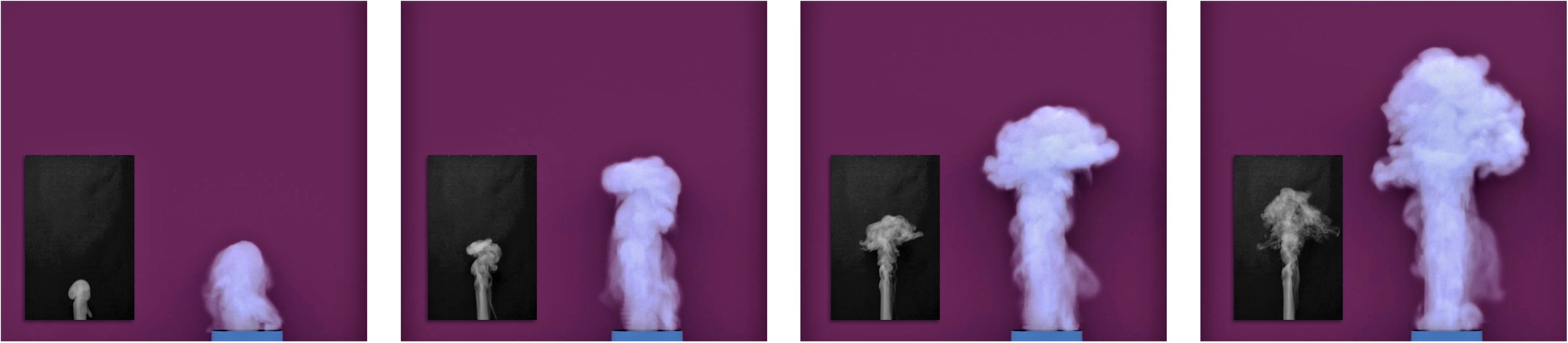
Figure 1. An example sequence of our ScalarFlow data set. Four frames of our data set are re-rendered as thick smoke. Insets of the corresponding frames of one of the captured video streams, i.e. the real-world reference, are shown in the lower left corners.

1. Introduction

Despite the long-standing success of physical simulations as tools for visual effects (VFX) production, there is a notable lack of benchmark cases and data sets for evaluating the simulated results. While other fields of research, such as computational photography and geometry processing, can rely on large image and model databases for evaluation as well as machine learning applications, simulations for visual effects typically are only evaluated in terms of visuals by a small number of experts. This is partially caused by the inherent difficulties of capturing real-world counterparts for the simulated phenomena. Typically, we are dealing with volumetric effects, such as clouds of smoke, liquids, or deformable bodies, that inherently require a full acquisition of the three-dimensional (3D) volume and its motion. Thus, it is crucial to obtain a 3D description of the configuration of a material and its velocity field in order to compare and align the corresponding simulated quantities.

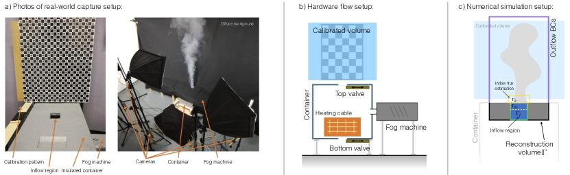
Figure 2. An overview of our capture setup: the container for smoke, calibration plate and camera setup (a), an illustration of the core components (b), and the corresponding numerical simulation and reconstruction domain (c).

In addition, the advent of data-driven methods, deep learning techniques in particular, has demonstrated the possibilities that arise from the availability of data sets. Most famously, the ImageNet data set (Deng et al., 2009) has been used in thousands of studies and led to huge advances for image classification. By now, many other data sets exist ranging from videos for action recognition (Abu-El-Haija et al., 2016) to 3D scenes for geometry reconstruction (Knapitsch et al., 2017). These data sets illustrate the potential for invigorating research, encouraging reproducible evaluations, and reducing the barrier of entry for newcomers. Overall, the availability of reliable data sets with sufficient complexity has led to significant progress of research in the corresponding fields. While first studies have successfully established connections between learning methods with physics-based simulations (Ladický et al., 2015; Chu and Thuerey, 2017; Ma et al., 2018), all of the studies so far purely rely on case-specific and synthetic (i.e., purely simulated) data.

Our goal with this work is to provide a first large-scale data set of real smoke clouds. The data was captured with a sparse, physics-based, multi-view tomography and contains volumetric reconstructions (i.e., velocity and density fields), video data, and camera calibrations. In addition, source code for capture and reconstruction will be published.

The primary contribution of our work is the creation of a carefully designed data set with a large number of accurate reconstructions of real-world scalar transport phenomena. Beyond this primary goal, our work contains several technical contributions: we propose the design of a low-cost hardware setup and an efficient optimization scheme for tomographic reconstructions. Our approach is able to recreate real-world smoke behavior even on modest resolutions by guiding a simulator along real-world footage and by employing an advanced method for estimating inflow boundary conditions. We also present, as a very first model application, a perceptual user study of different simulation methods and resolutions for buoyant smoke clouds based on our data set. Interestingly, these studies reveal that our reconstructions contain detail and natural dynamics that require forward simulations with very high resolutions in order to be matched.

2. Related Work

Scientific Data Sets have a long history in research, and a popular example from the computational fluid dynamics (CFD) community is the Johns Hopkins Turbulence Database. It contains eight very finely resolved simulations of different turbulent flows (Li et al., 2008). Despite being widely used for turbulence modeling, the data sets in this database focus on non-visual flows, i.e., without observable quantities, and contain a single data set for each of the eight setups. Hence, the data is not readily usable for graphics, vision, or deep learning applications. Other CFD and fluid flow databases, such as the THT Lab (Myong and Kasagi, 1990), KTH Flow (Schlatter and Orlu, 2010), and FDY DNS (Avsarkisov et al., 2014) databases, share these characteristics: they offer single simulated data sets with varying resolutions.

With our database, we target scalar transport processes in the form of buoyant plumes of hot smoke, which represent a large class of fluid problems in computer animation (Fedkiw et al., 2001a; Sato et al., 2018). At the same time, scalar transport phenomena are important for engineering (Moin et al., 1991; Yazdani et al., 2018) and medical applications (Morris et al., 2016) because the transported quantities yield important information about the flow motion. We specifically aim for providing many varied data sets of a single phenomenon, e.g., to support the construction of reduced models.

Fluid Simulations are important and established components in numerous fields (Harlow and Welch, 1965; Cummins et al., 2018). In graphics, a popular Eulerian, i.e. grid-based, solver for flow simulations is the Stable Fluids algorithm (Stam, 1999) and various extensions are available, e.g., to retain kinetic energy (Fedkiw et al., 2001b; Selle et al., 2005), to speed up the pressure projection component (McAdams et al., 2010; Setaluri et al., 2014), and to improve the accuracy of the advection step (Kim et al., 2005; Selle et al., 2008; Zehnder et al., 2018). For many VFX applications, guiding and control (Shi and Yu, 2005; Nielsen et al., 2009; Pan and Manocha, 2017) are highly important. In addition, the material point method has become a popular alternative for complex, fluid-like materials (Stomakhin et al., 2013; Jiang et al., 2016; Tampubolon et al., 2017), while the class of smoothed particle hydrodynamics methods represent purely Lagrangian variants (Ihmsen et al., 2014). Additionally, vortex filaments (Angelidis et al., 2006; Weißmann and Pinkall, 2010) are a popular Lagrangian representation for volumetric flows. We will focus on Eulerian solvers as they are widely used for single-phase smoke simulations. A thorough overview can be found in corresponding text books (Bridson, 2015). Note that while graphics publications typically refer to dense, passively advected tracers as smoke, our hardware setup diffuses water and, as such, produces fog. However, this is purely a difference in terminology; the underlying physics are equivalent. Thus, our setup is representative for the commonly used hot smoke simulations (Fedkiw et al., 2001b), and we will refer to the tracers as smoke from now on.

Flow Capture and Tomography: Fluid flows are inherently difficult to capture. While traditional experiments often perform only very localized measurements of quantities like pressure and velocity (Kavandi et al., 1990), methods such as particle image velocimetry (PIV) (Elsinga et al., 2006) can be used to recover volumetric information about flow motions by injecting particles. While specialized methods were able to recover 3D flows over time (Xiong et al., 2017), PIV cannot be employed in graphics settings as substances in the fluid such as smoke would immediately obscure the particles and the process is typically restricted to relatively small volumes.

While laser scanning setups (Hawkins et al., 2005), sheet-based reconstructions (Hasinoff and Kutulakos, 2007), and Schlieren-based capture algorithms (Atcheson et al., 2008; Atcheson et al., 2009) have been proposed, tomographic reconstructions are a more widely used alternative. In this case, external observations, typically in the form of two-dimensional (2D) images, are used to recover a 3D density. Beyond the medical field, such methods were successfully used to, e.g., reconstruct flames (Ihrke and Magnor, 2004, 2006) and nebulae (Wenger et al., 2013). Higher-level optimization involving tomographies were also proposed for the detailed capture of slowly deforming objects (Zang et al., 2018b; Zang et al., 2018a). We likewise make use of tomographic reconstructions from a sparse set of views, which are combined with physical constraints to obtain a realistic flow field. Algorithms employing physical simulations (or parts thereof) were successfully used in previous work to capture liquids (Wang et al., 2009), divergence-free motions (Gregson et al., 2014), and smoke volumes via appearance transfer (Okabe et al., 2015). Similar in spirit to our work, a physics-based single-view reconstruction was proposed (Eckert et al., 2018), which, however, lacks our procedure for inflow estimation and does not yield sufficiently reliable reconstructions due to being restricted to a single viewpoint.

Applications Areas: There are numerous potential areas of application for volumetric flow data sets in the areas of computer vision, graphics, and machine learning alone. To leverage machine learning in the context of simulations, researchers have, e.g., used machine learning to drive particle-based simulations (Ladický et al., 2015), replaced the traditional pressure solve with pre-trained models (Tompson et al., 2017), and augmented simulated data with learned descriptors (Chu and Thuerey, 2017). Others have focused on learning controllers for rigid body interactions (Ma et al., 2018) or aimed for temporal coherence with adversarial training (Xie et al., 2018). This is a nascent field with growing interest, where our data set can provide a connection of simulations with the real world. Although this is a promising direction, we will focus on evaluating the results of established simulation techniques in comparison to real-world flows as a first demonstration of the usefulness of a volumetric flow data set. Perceptual evaluations have been used to evaluate rendering algorithms (Cater et al., 2002), tone mapping (Masia et al., 2009), and animations of human characters (Hoyet et al., 2013). Recently, different methods for liquid simulations were also evaluated in regard to their visual realism (Um et al., 2017). However, to the best of our knowledge, no perceptual evaluations of the more fundamental algorithms for single-phase flows exist so far.

3. Method

In the following, we will outline the reconstruction algorithm that was used to create the ScalarFlow data set. A preview of our physical setup for capturing real-world smoke plumes is shown in Fig. 2 and will be explained in more detail in Sec. 4. Our goal is to jointly reconstruct smoke density $\Phi$ and velocity $\mathbf{u}$ from a small number of image sequences $i$. This represents an inverse problem as our goal is to find a solution of a numerical simulation that matches a set of observations. The widely established physical model for fluids are the incompressible Navier-Stokes equations, written as

(1) $$\frac{\partial\mathbf{u}}{\partial t}+\mathbf{u}\cdot\nabla\mathbf{u} =-\nabla p+\nu\triangle\mathbf{u}+\mathbf{f}_{\text{ext}}$$

$$\nabla\cdot\mathbf{u} =0,$$

where $\mathbf{u}$ is velocity, $p$ is pressure, $\mathbf{f}_{\text{ext}}$ are external body forces, and $\nu$ is kinematic viscosity. Typical simulators solve those equations for each time step $t$ via operator splitting: the velocity is advected forward, projected onto the divergence-free space via the so-called pressure solve, viscosity and external forces are added, and optionally, inflow quantities are added. A schematic overview can be found in Fig. 3(a). Note that common simulators often exhibit a limit on resolvable features and, as such, sub-grid effects such as turbulent mixing are not directly captured.

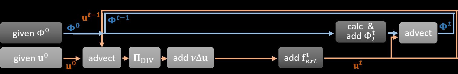
(a) Typical steps of a fluid simulator.

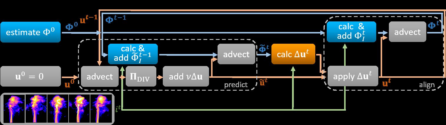
(b) Overview of our reconstruction method.

Figure 3. Visual summary of a typical forward fluid simulation and its inverse problem of recovering a simulation that matches a set of given target images. While we can re-use many steps from a regular simulator for the latter, i.e. advection, pressure projection, and viscosity, we need to estimate the unknown initial quantities, especially the 3D density, estimate a valid density inflow in compliance with the target images, and account for any unknown force.

It is inherently difficult to re-simulate real-world fluid phenomena as initial density distribution $\Phi^{0}$, density inflow $\Phi^{t}_{\text{I}}$, initial velocity $\mathbf{u}^{0}$, velocity inflow, and ambient air motions are unknown. External forces $\mathbf{f}_{\text{ext}}$ such as buoyancy are likewise typically difficult to model. Furthermore, simulators introduce numerical errors, which need to be counteracted, particularly for moderate domain resolutions, in order to reproduce the turbulent motion found in real-world smoke plumes. In this context, our approach shares similarities with methods for flow guiding (Nielsen et al., 2009; Pan et al., 2013). To match the real-world capture, we account for all unknown changes of velocities, i.e., forces, by calculating a residual velocity $\Delta\mathbf{u}^{t}$ and a density inflow $\Phi^{t}_{\text{I}}$.

Our full reconstruction algorithm is visualized in Fig. 3(b) and described in Appendix B in Alg. 3 with pseudocode. We also provide algorithms in pseudocode for all of the following steps. In our reconstruction algorithm, we first estimate the initial density volume $\Phi^{0}$ with a single pass of regular tomography and assume the fluid is initially at rest, i.e., $\mathbf{u}^{0}=0$. Then, in order to ensure temporal coherence, we predict velocity $\mathbf{\tilde{u}}^{t}$ by advecting the previous velocity $\mathbf{u}^{t-1}$ forward, making it divergence-free, and applying viscosity. To obtain a prediction for density, we calculate and add to $\Phi^{t-1}$ an inflow source $\tilde{\Phi}^{t}_{\text{I}}$ before advecting $\Phi^{t-1}$ with $\mathbf{\tilde{u}}^{t}$. Details of this step will be given in Sec. 3.3. The predicted density $\tilde{\Phi}^{t}$ is an intermediate variable that is only required to calculate the residual velocity, as shown in Fig. 3(b). Our reconstruction method proceeds by accounting for the residual velocity that is necessary to match the motion and shape from the input image sequences by computing $\Delta\mathbf{u}^{t}$. In an alignment step, $\Delta\mathbf{u}^{t}$ and $\mathbf{\tilde{u}}^{t}$ are accumulated to yield the final velocity $\mathbf{u}^{t}$. For computing the final density field $\Phi^{t}$, it is crucial to estimate the correct amount of inflow density $\Phi^{t}_{\text{I}}$, which is added to $\Phi^{t-1}$ before it is advected with $\mathbf{u}^{t}$ to finally obtain $\Phi^{t}$. It is important to emphasize that, similar to a regular forward simulation, the smoke density is solely changed via advection. We never modify densities outside the inflow region directly. We denote our reconstruction domain with $\Gamma$, while the inflow region is denoted with $\Gamma_{I}$, which is visualized in Fig. 2c. Outflow boundary conditions are set at the domain sides. Here velocity is allowed to move freely and densities in this region are removed.

3.1. Residual Velocity Estimation

We calculate a residual velocity $\Delta\mathbf{u}^{t}$ that moves the predicted density $\tilde{\Phi}^{t}$ such that the input images $i^{t}$ are matched. We denote the density change induced by $\Delta\mathbf{u}^{t}$ with $\Delta\Phi^{t}$. This change in density is an important intermediate variable required to enforce constraints on the density, which then constrains the residual velocity through our combined optimization scheme. As formulated in Eq. (2), we use the following physical assumptions for our reconstruction approach: residual velocity $\Delta\mathbf{u}^{t}$ and density $\Delta\Phi^{t}$ must comply with the transport equations; the total velocity inflow $\mathbf{\tilde{u}}^{t}|_{I}+\Delta\mathbf{u}^{t}|_{I}$ is equal to a constant $c$; the residual velocity field is incompressible; projecting the residual density back to each camera plane should be equal to the difference between input images $i^{t}$ and the current, projected density prediction $\tilde{i}^{t}$. Finally, the sum of residual and predicted density must be non-negative. This yields the following minimization problem:

(2) $$\underset{\Delta\Phi^{t},\Delta\mathbf{u}^{t}}{\text{minimize}} g(\Delta\mathbf{u}^{t},\Delta\Phi^{t})=\left\lVert\Delta\Phi^{t}+\nabla\tilde{\Phi}^{t}\cdot\Delta\mathbf{u}^{t}\right\rVert^{2}$$

subject to $$\mathbf{P}\>\Delta\Phi^{t}=i^{t}-\tilde{i}^{t},\;\Delta\Phi^{t}+\tilde{\Phi}^{t}\geq 0,$$

$$\Delta\mathbf{u}^{t}|_{I}=c-\mathbf{\tilde{u}}^{t}|_{I},\nabla\cdot\Delta\mathbf{u}^{t}=0,$$

where $\mathbf{P}$ is the matrix projecting 3D density back to each 2D image, the finite difference for $\frac{\partial\tilde{\Phi}^{t}}{\partial t}$ is denoted with $\Delta\Phi^{t}$, and $c$ is a constant approximating the average upwards speed of the observed flow. A detailed derivation of Eq. (2) can be found in Appendix C.

Following common practice (Parikh et al., 2014), we make our problem formulation convex by adding smoothness and kinetic energy regularizers for both density and velocity, namely

(3) $$E_{\text{smooth}}(\Delta\Phi^{t}) = \tfrac{1}{2}\left\lVert\nabla(\Delta\Phi^{t})\right\rVert^{2}, E_{\text{smooth}}(\Delta\mathbf{u}^{t}) = \tfrac{1}{2}\left\lVert\nabla\Delta\mathbf{u}^{t}\right\rVert^{2},$$

$$E_{\text{kin}}(\Delta\Phi^{t}) = \tfrac{1}{2}\left\lVert\Delta\Phi^{t}\right\rVert^{2}, E_{\text{kin}}(\Delta\mathbf{u}^{t}) = \tfrac{1}{2}\left\lVert\Delta\mathbf{u}^{t}\right\rVert^{2}.$$

The kinetic and smoothness regularizers are realized by adding a weighted diagonal and a Laplacian matrix to the system matrix, respectively. The Laplacian operator is discretized with central finite differences, yielding the standard 7-point stencil. We also regularize the density inflow. The weights for both regularizers depend on the actual values of density and velocity. In our case, we used ((1e-1, 5e-4), (6e-1, 5e-2), (5e-3, 1e-2)) for smoothness and kinetic regularizers for velocity, density, and inflow density, respectively.

We compute solutions for the residual velocity’s objective function $g(\Delta\Phi^{t},\Delta\mathbf{u}^{t})$ with least-squares and a standard Conjugate Gradient (CG) solver. As the shared objective function $g$ is convex and we have separate orthogonal projections for both unknowns $\Delta\Phi^{t}$ and $\Delta\mathbf{u}^{t}$, we use a fast primal-dual algorithm (PD) (Chambolle and Pock, 2011) to solve the joint optimization problem. The divergence-free constraint on the velocity is an orthogonal projection onto the space of divergence-free vector fields as shown in (Gregson et al., 2014). This is enforced via a regular pressure solver. Before enforcing incompressibility, we set our inflow residual velocity to the difference between the prescribed constant $c$ and the predicted velocity $\mathbf{\tilde{u}}^{t}$. In order to fulfill both constraints on the residual density $\Delta\Phi^{t}$, we project it onto the space of densities where the input images are matched and the total density is non-negative. This can be realized by computing a density correction $\Delta\Phi^{t}_{c}$, which is added to $\Delta\Phi^{t}$, as will be explained in Sec. 3.2. In line with optical flow (OF) methods (Meinhardt-Llopis et al., 2013), we solve for the residual velocity on multiple scales, i.e. employ a hierarchical approach as outlined in Alg. 6.

While previous work has attempted single-view reconstructions with a similar algorithm, we leverage the described physics-constrained optimization scheme for accurate multi-view tomographies. Using multiple views has the advantage that fewer unknown motions exist in the volume; thus, we do not need to employ the depth-regularization from previous work (Eckert et al., 2018). Next, we will explain our novel inflow estimation step and our efficient tomography scheme, which is important for obtaining feasible run times for the reconstruction.

3.2. Regularized Tomography

In order to satisfy both the image-matching and non-negativity constraints for the residual density $\Delta\Phi^{t}$, we add a correction $\Delta\Phi^{t}_{c}$ by solving a second minimization problem:

(4) $$\underset{\Delta\Phi^{t}_{c}}{\text{minimize}} h(\Delta\Phi^{t}_{c})=\left\lVert\mathbf{P}\Delta\Phi^{t}_{c}-{\color[rgb]{0,0,0}(i^{t}-\tilde{i}^{t}-\mathbf{P}\Delta\Phi^{t})}\right\rVert^{2}$$

subject to $$\Delta\Phi^{t}_{c}+\Delta\Phi^{t}+\tilde{\Phi}^{t}\geq 0,$$

where $\mathbf{P}$ is the matrix that projects from volume into image space, i.e., $\mathbf{P}\in\mathbb{R}^{n_{p}\times n_{v}}$; $n_{p}$ and $n_{v}$ denote the total number of pixels and voxels, respectively. We use a linear image formation model, where we integrate smoke densities along a ray. The tomography problem is solved with PD where pseudocode for is given in Appendix B in Alg. 4. When solving Eq. (4) with least-squares, it is necessary to calculate the matrix product $\mathbf{P}^{T}\mathbf{P}$. Because of the sparsity of the views, $n_{p}\ll n_{v}$ and $\mathbf{P}^{T}\mathbf{P}\in\mathbb{R}^{n_{v}\times n_{v}}$ is significantly larger and usually denser than $\mathbf{P}$. Hence, storing $\mathbf{P}^{T}\mathbf{P}$ explicitly is infeasible for larger resolutions due to excessive memory consumption. Therefore, we employ a CGLS solver (Ihrke and Magnor, 2004), which solves the normal equations like a regular CG solver but avoids computing $\mathbf{P}^{T}\mathbf{P}$ explicitly.

For under-determined inverse problems such as our sparse tomography, regularizers are crucial in order to obtain smooth and realistic density estimations as well as fluid motions. However, incorporating regularizers via a square and symmetric matrix, as commonly done for regular CG solvers, is not straightforward in CGLS. We show that regularizers and proximal operator extensions can be included in CGLS without the need for an explicit calculation of the system matrix.

A square regularization matrix $\mathbf{R}\in\mathbb{R}^{n_{v}\times n_{v}}$ for smoothness and kinetic energy is very sparse in practice: seven entries per row in 3D (diagonal and neighbours for smoothness, see Eq. (3)) suffice, and hence the matrix can be stored and multiplied efficiently. Within CGLS, it is necessary to only apply $\mathbf{R}$ to the residual and step size calculations. In order to use the CGLS solver as proximal operator within a PD optimization loop, we also need to add a weighted diagonal matrix $\sigma\mathbf{I}$ to the system matrix and the PD variable updates $\sigma\text{b}_{PD}$ to the right-hand side.

Algorithm 1 Regularized CGLS

1:function solveCGLSReg($\mathbf{P},\mathbf{R},\text{b},\text{b}_{PD},\sigma$)

2:     $\mathbf{r}_{0}=\sigma\text{b}_{PD}-\mathbf{P}^{T}\text{b}-\mathbf{P}^{T}\mathbf{P}x_{0}-(\mathbf{R}+\sigma\mathbf{I})x_{0}$;

3:     $\mathbf{p}_{0}=\mathbf{r}_{0}$;

4:     while accuracy not reached do

5:         $\alpha_{k}=\left\lVert\mathbf{r}_{k-1}\right\rVert^{2}/(\mathbf{p}_{k-1}^{T}\mathbf{P}^{T}\mathbf{P}\mathbf{p}_{k-1}+\mathbf{p}_{k-1}^{T}(\mathbf{R}+\sigma\mathbf{I})\mathbf{p}_{k-1})$;

6:         $\mathbf{x}_{k}=\mathbf{x}_{k-1}+\alpha_{k}\mathbf{p}_{k-1}$;

7:         $\mathbf{r}_{k}=\mathbf{r}_{k-1}-\alpha_{k}*\mathbf{P}^{T}\mathbf{P}\mathbf{p}_{k-1}+\alpha_{k}(\mathbf{R}+\sigma\mathbf{I})\mathbf{p}_{k-1};$

8:         $\beta_{k}=\left\lVert\mathbf{r}_{k}\right\rVert^{2}/\left\lVert\mathbf{r}_{k-1}\right\rVert^{2};$

9:         $\mathbf{p}_{k}=\mathbf{r}_{k}+\beta_{k}*\mathbf{p}_{k-1};$      

This regularized CGLS solve is summarized in Alg. 1 and used for all tomographic density reconstructions in our framework.

3.3. Inflow Estimation Solver

Suitable boundary conditions are crucial for all physical models and are likewise crucial for our reconstruction method. The unseen inflow region and its boundary with the visible domain have a huge influence on the overall reconstruction quality. Underestimating the density inflow will yield plumes that cannot fill the desired volume in later stages of the reconstruction, see Fig. 4a), while over-estimations can lead to strong instabilities over the course of the inverse solve, see Fig. 4c) for an example. We propose an approach for solving for the correct amount of density influx by computing the unseen inflow density $\Phi^{t}_{\text{I}}$ considering the previous density $\Phi^{t-1}$, the final velocity $\mathbf{u}^{t}$, and the target input images $i^{t}$. Our result is displayed in Fig. 4b) where our reconstruction features the right amount of density to fill the plume in a stable manner.

\begin{overpic}[width=433.62pt]{images/inflowFails}\put(1.0,1.0){{\color[rgb]{1,1,1}\small a)}}\put(34.5,1.0){{\color[rgb]{1,1,1}\small b)}}\put(68.0,1.0){{\color[rgb]{1,1,1}\small c)}}\end{overpic}

Figure 4. Example reconstructions with too less density inflow a), our inflow estimation b), and too much density inflow c).

Advecting previous and inflow density with the final velocity should result in a density field, the sum of which matches the amount of target smoke density $\Phi^{t}_{\text{tar}}$ that is prescribed by the 2D input images. The inflow density is hence used to fill the gap between current density and the target amount of density. Both of them only consider the visible domain $\Gamma\setminus\Gamma_{I}$, i.e., not the inflow region:

(5) $$\sum_{\Gamma\setminus\Gamma_{I}}\mathcal{A}(\Phi^{t-1}+\Phi^{t}_{\text{I}},\mathbf{u}^{t})\overset{!}{=}\sum_{\Gamma\setminus\Gamma_{I}}\Phi^{t}_{\text{tar}},$$

where $\mathcal{A}(\cdot,\mathbf{u}^{t})$ denotes advection with the known velocity $\mathbf{u}^{t}$ and $\Phi^{t}_{\text{tar}}$ is the density target. Based on $\mathbf{u}^{t}$, we set up a linear system of equations in order to estimate the inflow densities that lead to the desired density influx; i.e., we solve $\textbf{A}_{I}\Phi^{t}_{\text{I}}=$ b for $\Phi^{t}_{\text{I}}$. In $\textbf{A}_{I}$, we discretize the advection operator $\mathcal{A}$ via semi-Lagrangian advection. The right-hand-side b contains the missing density, which should be added to the domain through the inflow solver. Note that, as target domain, we only need to consider cells in the visible domain, which back-trace into the inflow area $\Gamma_{I}$, a region that we denote as $\Gamma_{R}$, as visualized in Fig. 2c). This is the only region influenced by advecting the inflow density $\Phi^{t}_{\text{I}}$. The subset $\Gamma_{R}$ of $\Gamma$ is back-traced into a part of the inflow region, which is denoted as $\Gamma_{RI}$ in the following. Hence, we set up $\textbf{A}_{I}$ to contain one equation for each density in $\Gamma_{RI}$ and b to contain a target value for each voxel in $\Gamma_{R}$. We additionally ensure that each cell of the total inflow density is non-negative. Negative density values never occur in reality, and we found such enforcement to be crucial for plausible and numerically stable reconstructions. To enforce the non-negativity constraint in conjunction with computing $\textbf{A}_{I}\Phi^{t}_{\text{I}}=$b, we solve for $\Phi^{t}_{\text{I}}$ with least-squares using smoothness and kinetic energy regularizers as for our main reconstruction above and employ the same convex optimization scheme (Chambolle and Pock, 2011).

Algorithm 2 Estimate inflow, such that Eq. (5) holds

1:function estimInfl($i^{t},\Phi^{t-1},\mathbf{u}^{t}$)

2:     $\Phi^{t}_{\text{tar}}=\textsc{reconDen}(i^{t},0)$; $\triangleright$ target density

3:     $\Delta\Phi^{t}_{\text{tar}}=\Phi^{t}_{\text{tar}}-\mathcal{A}(\Phi^{t-1},\mathbf{u}^{t})$; $\triangleright$ residual target density

4:     for $k\leftarrow 1,10$ do $\triangleright$ Prima-Dual iterations

5:         $\triangleright$ matrix $\mathbf{A}_{I}$ represents advecting cells from $\Gamma_{RI}$ to $\Gamma_{R}$

6:         $\triangleright$ $\textbf{A}=\mathbf{A}_{I}^{T}\mathbf{A}_{I},\mathbf{A}_{I}=\mathcal{A}(\Phi^{t}_{\text{I}},\mathbf{u}^{t})|_{\Gamma_{RI}\text{ to }\Gamma_{R}},$

7:         $\triangleright$ b: target missing density; $\mathcal{A}(\Phi^{t-1}+\Phi^{t}_{\text{I}},\mathbf{u}^{t})|_{\Gamma_{R}}\geq 0$

8:         $\triangleright$ $\text{b}=-\mathbf{A}_{I}^{T}\text{max }\left(\Delta\Phi^{t}_{\text{tar}}|_{\Gamma_{R}}+d,-\mathcal{A}(\Phi^{t-1},\mathbf{u}^{t})|_{\Gamma_{R}}\right)$

9:         $\qquad+\mathbf{x}^{k-1}+\sigma\mathbf{y}^{k-1}$

10:         $\mathbf{x}^{k}=\mathbf{x}^{k-1}+\sigma\mathbf{y}^{k-1}-\sigma\textsc{solveLSE}(\textbf{A},\text{b})$

11:         $\mathbf{z}^{k}=\Pi_{\text{NonNeg}}(\Phi^{t-1}+\mathbf{z}^{k-1}-\tau\mathbf{x}^{k})$;

12:         $\mathbf{y}^{k}=\mathbf{z}^{k}+\theta(\mathbf{z}^{k}-\mathbf{z}^{k-1})$;      

13:     $\textsc{extrapolateSrcValues}(\mathbf{z}^{k})$;

14:     return $\mathbf{z}^{k}$;

Pseudocode for the inflow estimation step is given in Alg. 2. Additional details can be found in Appendix B.1. We first project the target images $i^{t}$ into the volume to obtain a 3D density target $\Phi^{t}_{\text{tar}}$. The residual target density field $\Delta\Phi^{t}_{\text{tar}}$, i.e., the missing density, is then given by the difference of target density and the advected previous density. In order to ensure the correct density influx into the visible domain $\Gamma\setminus\Gamma_{I}$, the right-hand side vector b contains the total missing density, i.e., $\Delta\Phi^{t}_{\text{tar}}$. As b covers only a subset of the domain, i.e., $\Gamma_{R}$, we set each entry to the corresponding value in $\Delta\Phi^{t}_{\text{tar}}|_{\Gamma_{R}}$ plus an update $d$ that accounts for further density discrepancies in the rest of the domain, i.e., $\Delta\Phi^{t}_{\text{tar}}|_{\Gamma\setminus(\Gamma_{R}\cup\Gamma_{I})}$. As we are solving for an inflow update to the current inflow values in $\Phi^{t-1}$, we must ensure that $\mathcal{A}(\Phi^{t-1}+\Phi^{t}_{\text{I}},\mathbf{u}^{t})\geq 0$, which means b$\geq-\mathcal{A}(\Phi^{t-1},\mathbf{u}^{t})$, see line 8 of Alg. 2. We slightly extrapolate the inflow values in $\Gamma_{I}$ into cells that were excluded from the solve to ensure subsequent advection steps have full access to the densities (line 13 of Alg. 2).

As this solve only targets the inflow volume $\Gamma_{I}$, its cost is negligible compared to the rest of the optimization procedure. However, due to the non-linear nature of the overall optimization, it is a crucial component for obtaining realistic reconstructions.

4. Hardware Setup

In addition to the algorithmic pipeline described in the previous section, another important component of our framework is a commodity hardware setup to capture real-world fluid flows. Our strong physics-based constraints allow us to accurately capture complex flows with very simple hardware. In particular, complex camera calibration and synchronization are not required. We use an insulated box, which is heated to a chosen temperature in combination with a regular fog machine to fill the box with a fluid that can be tracked visually. A sketch of our setup is shown in Fig. 2b. Not surprisingly, conservation of volume holds for real fluids, and as such, it is crucial to control in- as well as outflow to and of the box. We use two servo-controlled valves at the top and bottom of the box, which are closed to fill the box with fog from the fog machine and opened when initiating a capture. In practice, our heating element can yield air temperatures of up to 60 degree Celsius (${}^{\circ}\text{C}$) without posing safety risks.

For camera calibration, we use a movable plate with ChArUco marker patterns that yield a dense ray calibration for the volume right above the box. After calibration, we cover the box and the background with a diffuse black cloth in order to maximize contrast of the visible fog. To record the fog, we use a set of five Raspberry Pi computers with attached cameras mounted on microphone stands. In total, the whole capture setup consists of hardware that is available for less than 1100 USD. Thus, in contrast to previously proposed hardware setups in graphics (Hawkins et al., 2005; Xiong et al., 2017), our setup can be recreated with a very moderate investment. Furthermore, other algorithms (Gregson et al., 2014) typically require larger numbers of synchronized and carefully calibrated cameras.

5. Evaluation

(a) Base simulation, front, $t=170$.

(b) Larger inflow area, front, $t=145$.

(c) $50~{}\%$ more buoyancy, front, $t=122$.

(d) High-resolution, front, $t=155$.

(e) Base simulation, side, $t=170$.

(f) Larger inflow area, side, $t=145$.

(g) $50~{}\%$ more buoyancy, side, $t=122$.

(h) High-resolution, side, $t=155$.

Figure 5. Four different synthetic smoke simulations. Each with ground truth density (left) and reconstructed density (right), with ground truth velocity (lower left) and reconstructed velocity (lower right), for front and side views. The high-resolution simulation and reconstruction in d) and h) are downsampled to facilitate visual comparison. We use our real-world calibration data to generate the synthetic input images and use our inflow estimation for reconstruction. Across varying simulation parameters as well as resolution, our reconstructions recover both density and motion accurately.

To evaluate the accuracy of our pipeline, we use a series of simulated data sets for which we have known ground truth values available for all quantities. We investigate the reconstruction accuracy for varied parameters and at varying resolutions. The perturbed parameters mimic the unknown behavior of real-world setups and, thus, can be used to assess the robustness of our reconstruction algorithm in practical settings. For each scenario, we vary the noise in the inflow density of the simulation five times such that we obtain five different instances for each synthetic case. We reconstruct all five instances and calculate the mean and standard deviation of peak signal-to-noise ratio (PSNR) for differences in density, velocity, and images.

5.1. Reconstruction Accuracy

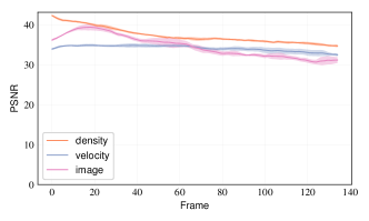
(a) Base simulation

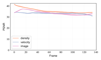
(b) Increased inflow area

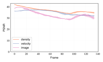
(c) Increased buoyancy

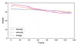
(d) Increased resolution

Figure 6. PSNR values of differences in density, velocity, and images for our four synthetic reconstructions in Fig. 5 with five different simulation and reconstruction instances each. We show the mean and standard deviation of PSNR values across the five instances.

First, we simulated a plume of hot smoke with the Boussinesq approximation at a resolution of $100\times 177\times 100$ and reconstructed the data set with the same resolution using our full algorithm. The plumes were rendered with our raycaster from five virtual views with real-world camera calibrations in line with our hardware setup. We then reconstructed the flow based on these images without using any additional information such as the ground truth inflow. The inflow was likewise computed with our estimation algorithm. This baseline comparison achieves a very high accuracy with averaged PSNR values of $37.3,34.1$, and $34.6$ for density, velocity and image differences, respectively, across all five instances, see Fig. 6a). A visual example can be found in Fig. 5a,e). Note that even the side view, which is heavily under-constrained in terms of visual observations, is reconstructed very accurately.

To evaluate the robustness of our method, we vary the size of the inflow source or increase the buoyancy force by $50\%$. Thus, in combination with the test above, these three tests yield distinct data points in the space of possible buoyant plume parameters. The resulting simulations exhibit significantly different flow behavior as observed in Fig. 9b,c). Despite these variations, our algorithm very accurately reconstructs the different flows in terms of both visual density and flow motion (bottom row of Fig. 5). The error measurements provide PSNR values comparable to the earlier test, i.e., an average of $35.7,33.3,33.8$ and $36.8,34.9,33.1$ for density, velocity, and image differences, respectively, across all five instances, see Fig. 6b,c). These tests indicate that our method is capable of accurately reconstructing a variety of different buoyant flows. For our scenario with increased buoyancy, a slight drop in PSNR values is observed around $t=95$. Due to the increased buoyancy, the smoke plumes rise much faster and, as such, leave the domain around $t=95$. In order to arrive at a setup that resembles the challenging real-world conditions, we also used a reduced resolution of $100\times 177\times 100$ for the reconstruction of a synthetic high-resolution simulation with a doubled resolution of $200\times 354\times 200$. Despite the inherently different resolution used for reconstruction, the result of our algorithm closely matches the ground truth for both density and velocity (Fig. 5d,h). The averaged PSNR values are $33.0,31.6,$ and $32.6$ for density, velocity, and image differences, respectively, across all five instances, see Fig. 6d).

While our reconstructions exhibit slightly less overall density, it accurately captures the intricate shapes of the complex reference flows as shown visually in Fig. 5 and measured through PSNR values, see Fig. 9. All four tests with five instances each robustly produce similar PSNR values for density, velocity, and images over multiple time steps. As reconstruction proceeds, the PSNR values slightly drop, but they yield high overall averages across all five instances. The decrease of the PSNR values over time can be explained by the flow becoming more complex over time and by occupying a larger volume of the domain. From these tests, we conclude that, with our strong physics-based optimization, five camera views are sufficient to constrain a simulation to recreate realistic flow motion according to given input images.

5.2. Alternative Methods

\begin{overpic}[width=433.62pt]{images/relWork}\put(2.0,54.0){{\color[rgb]{1,1,1}\footnotesize a) Tomo + OF: $V_{a}$}}\put(35.0,54.0){{\color[rgb]{1,1,1}\footnotesize b) Simplified: $V_{b}$}}\put(68.0,54.0){{\color[rgb]{1,1,1}\footnotesize c) Ours}}\end{overpic}

Figure 7. A visual comparison of three methods in terms of reconstructed densities: a) a divergence-free optical flow reconstruction based on tomographic densities from previous work, b) a simplified version of our solver, and c) our full method. Our full algorithm is needed to obtain a realistic and detailed flow field without artifacts.

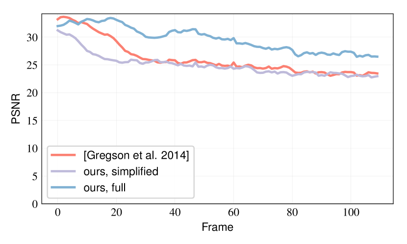
Figure 8. PSNR of image differences for $V_{a}$ (tomography plus 3D optical flow), $V_{b}$ (a simplified version of our approach), and our method.

In addition, we evaluate the gains in accuracy of our approach with respect to a flow reconstruction method from previous work and a simplified variant of our algorithm. The former approach, denoted as $V_{a}$ in the following, first computes volumetric densities through tomography and then applies 3D optical flow that is constrained to be divergence-free (in line with Gregson et al. (2014)). The second variant, denoted as $V_{b}$, uses our algorithm, but omits solving iteratively for an advection-aware residual density as outlined in Eq. (2), and instead uses a single delta density obtained from a separate tomography solve. The averaged PSNR values for image differences are $25.8,25.0,$ and $29.2$ for $V_{a},V_{b}$, and our method, respectively. These measurements show that our method reproduces the target input images with the highest accuracy among these methods, which is indicated by the per-time step PSNR measurements in Fig. 8. Although our method outperforms the others regarding error in the image space, there is more to consider as 2D error measurements cannot fully evaluate the quality of the volumetric reconstructions. Therefore, a qualitative evaluation in terms of densities is visualized in Fig. 7. As shown in Fig. 7a), the version $V_{a}$ exhibits the typical stripe artifacts from tomographic reconstructions leading to an overall lack of detail and clearly visible artifacts. Variant $V_{b}$ fares better as shown in Fig. 7b) but likewise lacks detail in the side view. Additionally, the reconstruction cannot keep up with the observations such that only two thirds of the overall length can be reconstructed. Our full algorithm shown in Fig. 7c) reconstructs the full sequence and develops natural, fluid-like behavior without tomography artifacts. These comparisons highlight that our iteratively re-computed density change is a density field that lies within the image formation null space and matches fluid motions significantly better than the updates computed by previous work. This improved quality is caused by the enhanced physical constraints which lead to a more realistic solution from the aforementioned null space. In this way, our method is able to produce more natural behavior and density configurations without the typical tomography artifacts and is especially suitable for under-constrained problems.

5.3. Performance

We also employ this setup to evaluate the performance of our optimized CGLS regularization. Here, a regular CG solver requires 535 seconds per tomography solve on average, while our CGLS solver achieves the same residual accuracy with only 69 seconds on average. While, for the regular CG, 182s are spent on the matrix construction, only 13s are required for CGLS. Thus, instead of being a bottleneck, the tomographic reconstruction becomes a smaller part of the overall run time, which was 809s and 350s on average per time step for CG and CGLS, respectively. Here, the performance of the CG version is indicative for the run times of previously proposed methods (Eckert et al., 2018).

In addition, the full CG solver requires approximately 15 GB of memory to store the tomography matrix $\mathbf{P}^{T}\mathbf{P}$, while the CGLS solver needs only 2.5 GB. As both memory and computational requirements grow super-linearly for larger resolutions, the regularized CGLS is crucial for obtaining reasonable run times for larger resolutions.

6. Data Set

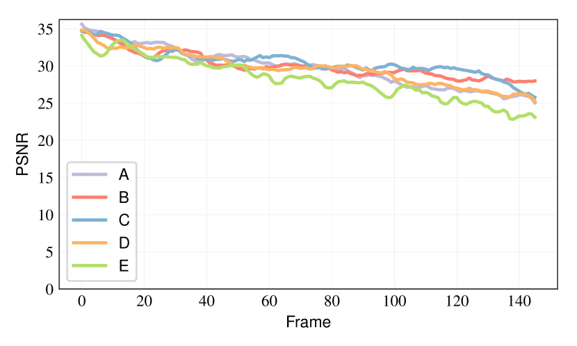
Figure 9. PSNR values of image differences for five different real-world reconstructions.

We now give an overview of the ScalarFlow data set, which is available online. The data set contains 100 flow reconstructions, each with a resolution of 100$\times$177$\times$100 and with at least 150 time steps (ca. 26 billion voxels of data in total). During the capture experiments, we used a temperature of $34^{\circ}~{}\text{C}$ as higher temperatures tend to move the visible flow too far out of the calibrated volume before producing interesting instabilities. This produces flow velocities of ca. 0.3 to 0.4$~{}\frac{\text{m}}{\text{s}}$ on average, once the fog plumes have accelerated. Naturally, the initial velocity for all captured flows is close to zero. Relative to the size of our calibrated capture volume of 0.9 m, this yields Reynolds numbers of up to ca. $5400$. Thus, the captured flows transition to turbulence during the later stages of each capture. In our reconstructions, we assume a viscosity of $1.516\cdot 10^{-5}~{}\frac{\text{m}^{2}}{\text{s}}$ for the fluid, and we record the rising plumes with $60$ fps.

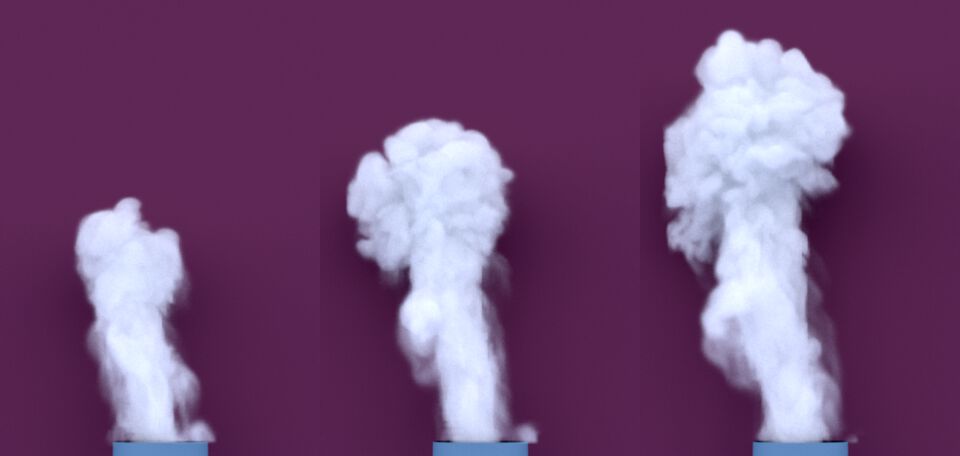
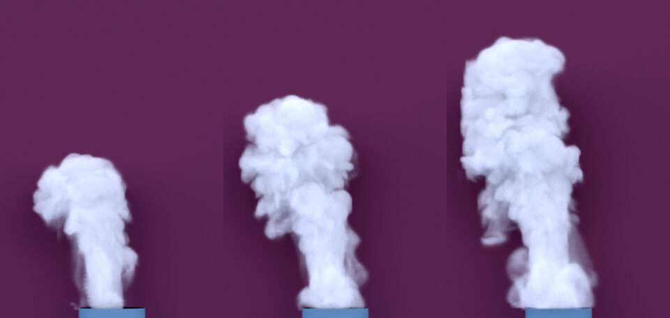
Figure 10. Four captured sequences shown in terms of thickly rendered reconstructed densities. Here, we visualize the captured plumes in a way that is very different to their real-world counterparts. This rendering style highlights the amount of small scale detail contained in our reconstructions.

Additional density and velocity visualizations for a selection of 20 reconstructions are shown in Fig. 14 in Appendix A. These visualizations show that our data set contains largely similar plume motions, which is important as our goal is to thoroughly sample a chosen space of physical behavior. However, despite the overall similarity, the captured flows contain a variety of interesting and natural variations, such as secondary plumes that form at various stages and separate from the main plume.

The volumetric velocity and density data contained in this collection can be flexibly used, e.g., for evaluations, re-simulations, data-driven applications, or visualizations. Example renderings of a sub-set of the density data are shown in Fig. 10. As for our comparison to alternative methods, we evaluate the accuracy of our real-world reconstructions by computing the PSNR between the captured images and the rendered reconstructed densities. As shown in Fig. 9, the images match the captured images very well with average PSNRs between $27.4$ and $29.7$. All five reconstructions robustly result in similar error ranges.

7. Perceptual Evaluation

As a first exemplary application of our data set, we show a perceptual evaluation of different simulation methods and resolutions for buoyant smoke clouds via user studies. To achieve robust and reliable evaluation results in these studies, a key requirement is to have reference data that can serve as ground truth and to have a large number of available data variants of the same phenomenon in order to increase robustness. For our user studies, we adopt the two-alternative forced choice (2AFC) design (Fechner, 1860) and compute scores with the Bradley-Terry model (Hunter, 2004; Um et al., 2017). We recruited 189 participants from 48 countries via crowd-sourcing, where each participant answered the randomized questions twice. In total, we had 100 answers per question to obtain statistically relevant result.

We first consider a selection of fluid solvers that are well established in the community in order to evaluate how closely their results resemble a real fluid. To this end, we selected four representative methods: semi-Lagrangian advection (Stam, 1999), MacCormack (Selle et al., 2008), advection-reflection (Zehnder et al., 2018), and wavelet turbulence (Kim et al., 2008) as a representative of up-res methods. While these methods have been compared visually in the corresponding publications, to the best of our knowledge, no evaluation of these methods in comparison to a real-world reference exists.

We implemented all simulation methods in the same solver framework (Thuerey and Pfaff, 2018) such that all four simulation variants use the same initial conditions and a resolution of 100$\times$177$\times$100. The base resolution of the wavelet turbulence version was halved such that the synthetic turbulence can be added with a two times up-sampling. Fig. 12 shows example frames of the four different simulations as well as one of our reconstruction data set.

The result of our 2AFC user study with the different methods is summarized in Fig. 1313(a). Our study shows which method resembles a real smoke cloud more closely. For instance, our evaluations show a chance of 64% that viewers prefer the advection-reflection version over the MacCormack result in comparison to our reconstruction.

It is typically crucial to have full control over the setup of the user studies. With the available 3D density of our data set, we are able to flexibly design our psychophysical studies with custom background, smoke color, rendering style, and viewing angles. Furthermore, thanks to the variety of reconstructions in the ScalarFlow data set, we can evaluate the aforementioned methods in comparison to multiple real flows. Despite their different behaviors, a range of salient flow features appears across these smoke clouds. In this way, we can determine the viewer’s preferences for a wider range of natural flow behavior, and we can ensure that a singular result is not an outlier. Conducting four additional user studies for the same method yet with different reference data, we found that the results of these studies were all highly correlated, $\rho\simeq 0.98$ $(P\simeq 0.02)$ on average, where $\rho$ and $P$ are the correlation coefficient and its p-value, respectively. This indicates that our evaluation results are stable. The joint preferences of our participants, computed across all four studies, are shown in red in Fig. 1313(a). Interestingly, the relatively old, procedural wavelet turbulence method exhibits a performance that is comparable to the advection-reflection solver and slightly outperforms the MacCormack scheme.

Figure 11. Example frames of user study videos for four different simulation methods, and one ScalarFlow data set. F.l.t.r.: Semi-Lagrangian, MacCormack, advection-reflection, wavelet turbulence, and ScalarFlow data.

Figure 12. Example frames of user study videos for increasing resolutions. The simulations with MacCormack advection for 1$\times$, 2$\times$, 4$\times$, 8$\times$, and 12$\times$ are shown from left to right, respectively.

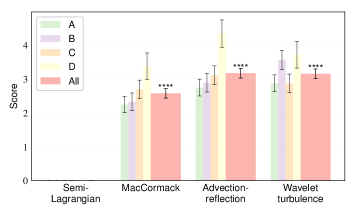
(a) Different methods

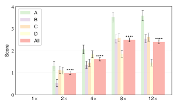
(b) Different resolutions

Figure 13. Evaluations of different simulation methods and different resolutions via user studies. (13(a)) Multiple evaluations (i.e., A, B, C, and D) of the same four methods are shown as well as their combined evaluation (i.e., All). In (13(b)) the evaluation of different resolutions is shown. ****$P<0.0001$.

In addition to the different simulation methods, we further investigate the influence of simulation resolution. As graphics solvers typically do not explicitly add viscosity, they rely on unknown amounts of numerical viscosity in order to achieve a realistic look. With this study, our goal was to investigate how much numerical viscosity is actually necessary to realistically simulate a plume of buoyant smoke approximately one meter high. Here, we focus on the MacCormack method as a de facto standard advection scheme, which we use to simulate five different resolutions. Starting with a resolution of 50$\times$88$\times$50 as the base resolution (i.e., 1$\times$), we increase the resolution by 2$\times$, 4$\times$, 8$\times$, and 12$\times$, respectively, arriving at 600$\times$1062$\times$600 for the most finely resolved version with 12$\times$. Note that we use a scaling factor of $1.77$ for the domain’s height. Example frames are shown in the supplemental material in Fig. 12.

Our user study, summarized in Fig. 1313(b), shows that the 8$\times$ and 12$\times$ resolutions are those that are considered to be closest to our captures. Interestingly, there is a noticeable variance in the evaluations across the different data sets. For version D, the 8$\times$ simulation is even considered to be closer to the capture than the 12$\times$ simulation. This behavior illustrates the need for a large number of data sets in order to ensure a robust evaluation. This result additionally shows that large resolutions are required in numerical simulations to perceptually match the behavior of real-world smoke clouds at a scale of ca. 90 cm. Consequently, larger real-world clouds would require even larger resolutions.

8. Limitations

Our reconstruction algorithm is a non-linear optimization procedure, and as such, is not guaranteed to converge. However, this is a limitation that our method shares with all previous work in this area. We found the algorithm to be stable in practice, but substantial changes in the data, like speed or brightness, can lead to diverging reconstruction runs. Here, a promising avenue for future work would be a further improved estimation of the inflow velocity and an automated adjustment of the reconstruction parameters, which could lead to even more accurate reconstructions.

In practice, the ambient air motion of our capture stage makes it difficult to fine-tune the direction of the plumes. Right now, applications of our data set have to include slight variations in terms of the overall plume direction. However, the data could be clustered with respect to average motions of the plume, and future extensions of the data set could yield enough samples such that individual directions of motion could be targeted.

In addition, we currently rely on a linear image formation model. While we found this to yield very good results for the relatively thin clouds of our fog machine, the linear image formation model would not be directly applicable to denser volumes.

9. Conclusions

We have shown that it is possible to accurately capture complex flows of scalar transport phenomena with a combination of commodity hardware and powerful physics-constrained reconstructions. Our reconstruction method with its inflow solver and efficient tomography routine are crucial for achieving this goal. The resulting algorithm allowed us to assemble a first large-scale data set of realistic flows. Our data set contains a unique combination of volumetric data for turbulent flows in conjunction with visual data and processing algorithms. In addition, our perceptual application demonstrated the usefulness of the reconstructed data and led to first insights regarding smoke simulation methods as well as the reconstruction itself. The studies show that the advection-reflection solver as well as the wavelet turbulence model perform best among the set of evaluated methods and our reconstructed flows contain dynamics that are comparable to finely resolved simulations.

The availability of a large, volumetric data set opens up a wide range of possibilities. In particular, the availability of velocities in our reconstructions means that the data can be flexibly used for re-simulations, novel visualization, incorporation into VFX scenes, and metric evaluations, e.g., in order to compare motions. Looking ahead, we believe that there is a wide range of exciting future applications for our data. Beyond avenues for benchmarking, accuracy measurements, and novel reconstruction methods, we are looking forward to developments in the area of machine learning that this data will enable (Sato et al., 2018; Xie et al., 2018; Kim et al., 2019).

Appendix A Additional Reconstructions

Figure 14. A sub-set of captured clouds of the ScalarFlow data set visualized in terms of density and velocity. Each row on both columns shows four frames of a single capture.

Appendix B Details of Reconstruction Algorithm

In this appendix, we outline our reconstruction algorithm with pseudocode where Alg. 3 is the main routine. Based on an initial density estimate, it iteratively predicts the quantities’ states and computes density inflow as well as a physics-constrained update to the velocities. The tomography solve in Alg. 4 is used for initialization and as a building block within the residual velocity calculation step of Alg. 5. Lastly, Alg. 6 details our recursive multi-scale version of the residual velocity computation, which makes use of Alg. 5.

We add our smoothness and kinetic energy regularizers described in Eq. (3) to matrix A for each linear system of equations (LSE) referred to in $\textsc{solveLSE}(\textbf{A},\text{b})$, i.e., for density and velocity in
$\textsc{reconDen}(i^{t},\tilde{\Phi}^{t}),$ $\textsc{reconVel}(\mathbf{\tilde{u}}^{t},\tilde{\Phi}^{t},i^{t}),$ and $\textsc{estimInfl}(i^{t},\Phi^{t-1},\mathbf{u}^{t})$. Furthermore, in order to apply PD, a weighted identity matrix $\sigma\textbf{I}$ is added as well.

Algorithm 3 Full Reconstruction Procedure

1:function reconVelDen($i^{t}$)$\triangleright$ reconstr. velocity and density

2:    $\mathbf{u}^{0}=0$; $\triangleright$ init velocity

3:    $\Phi^{0}=\textsc{reconDen}(i^{0},0)$; $\triangleright$ init density, Eq. (19)

4:    for all t do

5:         $\triangleright$ predict velocity

6:         $\mathbf{\tilde{u}}^{t}=\Pi_{\text{DIV}}(\mathcal{A}(\mathbf{u}^{t-1},\mathbf{u}^{t-1}))+\textsc{addViscosity}(\mathbf{u}^{t-1})$;

7:         $\tilde{\Phi}^{t}_{\text{I}}=\textsc{estimInfl}(i^{t},\Phi^{t-1},\mathbf{\tilde{u}}^{t})$; $\triangleright$ estimate density inflow

8:         $\tilde{\Phi}^{t}=\mathcal{A}(\Phi^{t-1}+\tilde{\Phi}^{t}_{\text{I}},\mathbf{\tilde{u}}^{t})$; $\triangleright$ predict density

9:         $\triangleright$ solve for residual velocity Eq. (2)

10:         $\Delta\mathbf{u}^{t}=\textsc{reconVelMS}(\mathbf{\tilde{u}}^{t},\tilde{\Phi}^{t},\Phi^{t-1},i^{t})$;

11:         $\mathbf{u}^{t}=\mathbf{\tilde{u}}^{t}+\Delta\mathbf{u}^{t}$; $\triangleright$ finalize velocity

12:         $\Phi^{t}_{\text{I}}=\textsc{estimInfl}(i^{t},\Phi^{t-1},\mathbf{u}^{t})$; $\triangleright$ estimate density inflow

13:         $\Phi^{t}=\mathcal{A}(\Phi^{t-1}+\Phi^{t}_{\text{I}},\mathbf{u}^{t})$; $\triangleright$ finalize density     

Algorithm 4 Tomography, solve Eq. (19), (20), or (21)

1:function reconDen($i^{t},\Phi_{\text{IN}}^{t}$)$\triangleright$ reconstr. density, $\Phi_{\text{IN}}^{t}$ can be 0

2:    $\Delta i^{t}=i^{t}-\mathbf{P}\Phi_{\text{IN}}^{t}$; $\triangleright$ calculate residual image

3:    for $k\leftarrow 1,10$ do $\triangleright$ Prima-Dual iterations

4:         $\triangleright$ solve least-squares problem, e.g., with CGLS (Alg. 1)

5:         $\mathbf{x}^{k}=\mathbf{x}^{k-1}+\sigma\mathbf{y}^{k-1}$

6:         $\quad-\sigma\textsc{solveLSE}(\textbf{A}=\mathbf{P}^{T}\mathbf{P},\text{b}=-\mathbf{P}^{T}\Delta i^{t}+\mathbf{x}^{k-1}+\sigma\mathbf{y}^{k-1})$;

7:         $\mathbf{z}^{k}=\Pi_{\text{NonNeg}}(\Phi_{\text{IN}}^{t}+\mathbf{z}^{k-1}-\tau\mathbf{x}^{k})$; $\triangleright$ cut off neg. values

8:         $\mathbf{y}^{k}=\mathbf{z}^{k}+\theta(\mathbf{z}^{k}-\mathbf{z}^{k-1})$;     

9:    return $\mathbf{z}^{k}$;

Algorithm 5 Residual Velocity, solve Eq. (2)

1:$\triangleright$ calculate residual velocity on single scale

2:function reconVel($\mathbf{\tilde{u}}^{t},\tilde{\Phi}^{t},i^{t}$)

3:    for $k\leftarrow 1,10$ do $\triangleright$ Prima-Dual iterations

4:         $\triangleright$ shared part: advection equation, $\mathbf{x}^{k}=\mathbf{x}_{\mathbf{u}}^{k}\cup\mathbf{x}_{\Phi}^{k}$

5:         $\mathbf{x}^{k}=\mathbf{x}^{k-1}+\sigma\mathbf{y}^{k-1}-\sigma\textsc{solveLSE}(\textbf{A},\text{b})$;

6:         $\triangleright$ $\textbf{A}=\begin{bmatrix}(\nabla\tilde{\Phi}^{t})(\nabla\tilde{\Phi}^{t})^{T}&(\nabla\tilde{\Phi}^{t})\\ (\nabla\tilde{\Phi}^{t})^{T}&I\end{bmatrix},\text{b}=\mathbf{x}^{k-1}+\sigma\mathbf{y}^{k-1}$

7:         $\triangleright$ velocity part: inflow and divergence-free on $\mathbf{z}_{\mathbf{u}}^{k}$

8:         $\Delta\mathbf{u}^{t}_{\text{tmp}}=\mathbf{z}_{\mathbf{u}}^{k-1}-\tau\mathbf{x}_{\mathbf{u}}^{k}$; $\triangleright$ create temporary velocity

9:         $\Delta\mathbf{u}^{t}_{\text{tmp}}|_{I}=c-\mathbf{\tilde{u}}^{t}|_{I}$; $\triangleright$ set velocity inflow

10:         $\mathbf{z}_{\mathbf{u}}^{k}=\Pi_{\text{DIV}}(\Delta\mathbf{u}^{t}_{\text{tmp}})$; $\triangleright$ make div-free

11:         $\triangleright$ density part: tomo. and non-neg. (Eq. (21)) on $\mathbf{z}_{\Phi}^{k}$

12:         $\mathbf{z}_{\Phi}^{k}=\mathbf{z}_{\Phi}^{k-1}-\tau\mathbf{x}_{\Phi}^{k}+\textsc{reconDen}(i^{t},\tilde{\Phi}^{t}+\mathbf{z}_{\Phi}^{k-1}-\tau\mathbf{x}_{\Phi}^{k})$;

13:         $\triangleright$ shared variable update, $\mathbf{y}^{k}=\mathbf{y}_{\mathbf{u}}^{k}\cup\mathbf{y}_{\Phi}^{k}$

14:         $\mathbf{y}^{k}=\mathbf{z}^{k}+\theta(\mathbf{z}^{k}-\mathbf{z}^{k-1})$;     

15:    return $\mathbf{z}_{\mathbf{u}}^{k}$;

Algorithm 6 MS Residual Velocity, solve Eq. (2)

1:$\triangleright$ calculate residual velocity on multiple scales

2:function reconVelMS($\mathbf{\tilde{u}}^{t},\tilde{\Phi}^{t},\Phi^{t-1},i^{t}$)

3:    if grid size large enough then

4:         $\Delta\mathbf{u}^{t}_{\text{C}}=\Pi_{\text{DIV}}(\textsc{up}(\textsc{reconVelMS}(\textsc{down}(\mathbf{\tilde{u}}^{t}),\textsc{down}(\tilde{\Phi}^{t}),i^{t})))$;

5:         $\mathbf{\tilde{u}}^{t}_{\text{new}}=\mathbf{\tilde{u}}^{t}+\Delta\mathbf{u}^{t}_{\text{C}}$; $\triangleright$ add coarse residual to prediction

6:         $\tilde{\Phi}^{t}_{\text{I,new}}=\textsc{estimInfl}(i^{t},\Phi^{t-1},\mathbf{\tilde{u}}^{t}_{\text{new}})$; $\triangleright$ den. inflow

7:         $\tilde{\Phi}^{t}_{\text{new}}=\mathcal{A}(\Phi^{t-1}+\tilde{\Phi}^{t}_{\text{I,new}},\mathbf{\tilde{u}}^{t}_{\text{new}})$; $\triangleright$ adapt prediction

8:         $\triangleright$ sum up residual velocities on different scales

9:         $\Delta\mathbf{u}^{t}=\Delta\mathbf{u}^{t}_{\text{C}}+\textsc{reconVel}(\mathbf{\tilde{u}}^{t}_{\text{new}},\tilde{\Phi}^{t}_{\text{new}},i^{t})$;

10:    else

11:         $\Delta\mathbf{u}^{t}=\textsc{reconVel}(\mathbf{\tilde{u}}^{t},\tilde{\Phi}^{t},i^{t})$;     

12:    return $\Delta\mathbf{u}^{t}$;

B.1. Visual Hull and Inflow Estimation

For the density estimation (both tomography and inflow), we incorporate a visual hull to achieve higher accuracy and reduce computational complexity. Inflow source cells from $\Gamma_{RI}$ are set to zero and excluded from the solve in order to prevent density in cells that should be empty. We only mark them as outside if the contributing weight is above 1e-2, while voxels are included in the system if their weight is above 1e-4. These thresholds were determined experimentally for our hardware setup and were used for all of our reconstructions.

Regarding the density discrepancy $d$ for the inflow solve, we could distribute the total missing residual density from $\Delta\Phi^{t}_{\text{tar}}|_{\Gamma\setminus(\Gamma_{R}\cup\Gamma_{I})}$ (positive or negative) equally to each target cell, i.e.,

$$d=\frac{\sum\limits_{\Gamma\setminus(\Gamma_{R}\cup\Gamma_{I})}\Delta\Phi^{t}_{\text{tar}}}{|\Gamma_{R}|}.$$

However, we instead choose to scale the value $d$ with the value in $\Delta\Phi^{t}_{\text{tar}}|_{\Gamma_{R}}$ such that a cell $e\in\Gamma_{R}$ with truly higher values gets a larger fraction of the missing densities assigned, i.e.,

$$d_{e}=\frac{\sum\limits_{\Gamma\setminus(\Gamma_{R}\cup\Gamma_{I})}\Delta\Phi^{t}_{\text{tar}}}{\sum\limits_{\Gamma_{R}}(\Delta\Phi^{t}_{\text{tar}}+\text{o})}(\Delta\Phi^{t}_{\text{tar}}|_{e}+\text{o}),$$

where the offset o ensures that each $\Delta\Phi^{t}_{\text{tar}}|_{e}\geq 0$ for scaling. We additionally require cells with negative values to contain less density than the positive ones. Accordingly, the offset is 0 or the absolute value of the largest negative entry in $\Delta\Phi^{t}_{\text{tar}}|_{\Gamma_{R}}$, i.e., $\text{o}=|\text{min}(0,\Delta\Phi^{t}_{\text{tar}}|_{\Gamma_{R}})|$.

Appendix C Derivation of Optimization Problem

In this section, we derive our optimization problem for the residual velocity step-by-step:

(7) $$\underset{\mathbf{u}^{t},\Phi^{t}}{\text{minimize}} \left\lVert\frac{\partial\Phi^{t}}{\partial t}+\nabla\Phi^{t}\cdot\mathbf{u}^{t}\right\rVert^{2}$$

$$\qquad\qquad\qquad\left|\begin{array}[]{l}\Phi^{t}=\mathcal{A}(\Phi^{t-1}+\Phi^{t}_{\text{I}},\mathbf{u}^{t}),\\ \mathbf{u}^{t}=\mathbf{\tilde{u}}^{t}+\Delta\mathbf{u}^{t}\\ \end{array}\right.$$

$$\equiv\; \underset{\Delta\mathbf{u}^{t},\Phi^{t}_{\text{I}}}{\text{minimize}} \left\lVert\frac{\partial\mathcal{A}(\Phi^{t-1}+\Phi^{t}_{\text{I}},\mathbf{\tilde{u}}^{t}+\Delta\mathbf{u}^{t})}{\partial t}+\nabla\mathcal{A}(\Phi^{t-1}+\Phi^{t}_{\text{I}},\mathbf{\tilde{u}}^{t}+\Delta\mathbf{u}^{t})\cdot(\mathbf{\tilde{u}}^{t}+\Delta\mathbf{u}^{t})\right\rVert^{2}$$

$$\qquad\qquad\qquad\left|\begin{array}[]{l}\text{linearize advection}:\\ \mathcal{A}(\mathcal{A}(\Phi^{t-1}+\Phi^{t}_{\text{I}},\mathbf{\tilde{u}}^{t}),\Delta\mathbf{u}^{t})\approx\mathcal{A}(\Phi^{t-1}+\Phi^{t}_{\text{I}},\mathbf{\tilde{u}}^{t}+\Delta\mathbf{u}^{t})\\ \end{array}\right.$$

(10) $$\equiv\; \underset{\Delta\mathbf{u}^{t},\Phi^{t}_{\text{I}}}{\text{minimize}} \left\lVert\frac{\partial\mathcal{A}(\mathcal{A}(\Phi^{t-1}+\Phi^{t}_{\text{I}},\mathbf{\tilde{u}}^{t}),\Delta\mathbf{u}^{t})}{\partial t}+\nabla\mathcal{A}(\mathcal{A}(\Phi^{t-1}+\Phi^{t}_{\text{I}},\mathbf{\tilde{u}}^{t}),\Delta\mathbf{u}^{t})\cdot(\mathbf{\tilde{u}}^{t}+\Delta\mathbf{u}^{t})\right\rVert^{2}$$

$$\qquad\qquad\qquad\left|\begin{array}[]{l}\tilde{\Phi}^{t}_{\text{I}}=\Phi^{t}_{\text{I}},\\ \nabla\tilde{\Phi}^{t}\approx\nabla\Phi^{t}\\ \end{array}\right.$$

(12) $$\equiv\; \underset{\Delta\mathbf{u}^{t},\Phi^{t}}{\text{minimize}} \left\lVert\frac{\partial\mathcal{A}(\mathcal{A}(\Phi^{t-1}+\tilde{\Phi}^{t}_{\text{I}},\mathbf{\tilde{u}}^{t}),\Delta\mathbf{u}^{t})}{\partial t}+\nabla\mathcal{A}(\Phi^{t-1}+\tilde{\Phi}^{t}_{\text{I}},\mathbf{\tilde{u}}^{t})\cdot(\mathbf{\tilde{u}}^{t}+\Delta\mathbf{u}^{t})\right\rVert^{2}$$

$$\qquad\qquad\qquad\left|\begin{array}[]{l}\tilde{\Phi}^{t}=\mathcal{A}(\Phi^{t-1}+\tilde{\Phi}^{t}_{\text{I}},\mathbf{\tilde{u}}^{t}),\\ \text{remove constant terms}\\ \end{array}\right.$$

$$\equiv\; \underset{\Delta\mathbf{u}^{t},\Phi^{t}}{\text{minimize}} \left\lVert\frac{\partial\mathcal{A}(\tilde{\Phi}^{t},\Delta\mathbf{u}^{t})}{\partial t}+\nabla\tilde{\Phi}^{t}\cdot\Delta\mathbf{u}^{t}\right\rVert^{2}$$

$$\qquad\qquad\qquad\left|\begin{array}[]{l}\Delta\Phi^{t}=\frac{\partial\mathcal{A}(\tilde{\Phi}^{t},\Delta\mathbf{u}^{t})}{\partial t}=\frac{\tilde{\Phi}^{t}+\Delta\Phi^{t}-\,\tilde{\Phi}^{t}}{\Delta t},\Delta t=1\\ \end{array}\right.$$

$$\equiv\; \underset{\Delta\mathbf{u}^{t},\Delta\Phi^{t}}{\text{minimize}} \left\lVert\Delta\Phi^{t}+\nabla\tilde{\Phi}^{t}\cdot\Delta\mathbf{u}^{t}\right\rVert^{2}$$

subject to $$\mathbf{u}^{t}|_{I}=c\qquad\qquad\qquad\!\left|\;\mathbf{u}^{t}=\mathbf{\tilde{u}}^{t}+\Delta\mathbf{u}^{t},\text{ where {c} is inflow speed}\right.$$

$$\equiv\; \mathbf{\tilde{u}}^{t}|_{I}+\Delta\mathbf{u}^{t}|_{I}=c\qquad\left|\;\mathbf{\tilde{u}}^{t}\text{ is div-free}\right.$$

$$\equiv\; \Delta\mathbf{u}^{t}|_{I}=c-\mathbf{\tilde{u}}^{t}|_{I},$$

$$\nabla\cdot\mathbf{u}^{t}=0\qquad\qquad\qquad\!\left|\;\mathbf{u}^{t}=\mathbf{\tilde{u}}^{t}+\Delta\mathbf{u}^{t}\right.$$

$$\equiv\; \nabla\cdot(\mathbf{\tilde{u}}^{t}+\Delta\mathbf{u}^{t})=0\qquad\left|\;\mathbf{\tilde{u}}^{t}\text{ is div-free}\right.$$

$$\equiv\; \nabla\cdot\Delta\mathbf{u}^{t}=0,$$

$$\mathbf{P}\Phi^{t}-i^{t}=0\qquad\left|\;\Phi^{t}=\mathcal{A}(\Phi^{t-1}+\Phi^{t}_{\text{I}},\mathbf{u}^{t})\right.$$

$$\equiv\; \mathbf{P}\mathcal{A}(\Phi^{t-1}+\Phi^{t}_{\text{I}},\mathbf{u}^{t})-i^{t}=0\qquad\left|\;\mathbf{u}^{t}=\mathbf{\tilde{u}}^{t}+\Delta\mathbf{u}^{t},\tilde{\Phi}^{t}_{\text{I}}\approx\Phi^{t}_{\text{I}},\text{ lin. adv.}\right.$$

$$\equiv\; \mathbf{P}\mathcal{A}(\mathcal{A}(\Phi^{t-1}+\tilde{\Phi}^{t}_{\text{I}},\mathbf{\tilde{u}}^{t}),\Delta\mathbf{u}^{t})-i^{t}=0\qquad\left|\;\tilde{\Phi}^{t}=\mathcal{A}(\Phi^{t-1}+\tilde{\Phi}^{t}_{\text{I}},\mathbf{\tilde{u}}^{t})\right.$$

$$\equiv\; \mathbf{P}\mathcal{A}(\tilde{\Phi}^{t},\Delta\mathbf{u}^{t})-i^{t}=0\qquad\left|\;\mathcal{A}(\tilde{\Phi}^{t},\Delta\mathbf{u}^{t})=\tilde{\Phi}^{t}+\Delta\Phi^{t}\Rightarrow\Phi^{t}\approx\tilde{\Phi}^{t}+\Delta\Phi^{t}\right.$$

$$\equiv\; \mathbf{P}\tilde{\Phi}^{t}+\mathbf{P}\Delta\Phi^{t}-i^{t}=0,\qquad\left|\;\tilde{i}^{t}=\mathbf{P}\tilde{\Phi}^{t}\right.$$

$$\equiv\; \mathbf{P}\Delta\Phi^{t}-(i^{t}-\tilde{i}^{t})=0,\qquad\left|\;\Delta i^{t}=i^{t}-\tilde{i}^{t}\right.$$

$$\equiv\; \mathbf{P}\Delta\Phi^{t}-\Delta i^{t}=0,$$

$$\Phi^{t}\geq 0\qquad\qquad\qquad\left|\;\Phi^{t}\approx\tilde{\Phi}^{t}+\Delta\Phi^{t}\right.$$

$$\equiv\; \tilde{\Phi}^{t}+\Delta\Phi^{t}\geq 0$$

(18) $$\equiv\; \Delta\Phi^{t}\geq-\tilde{\Phi}^{t}.$$

The problem formulations for calculating density, residual density, or density correction are

(19) $$\underset{\Phi^{t}}{\text{minimize}}\left\lVert P\Phi^{t}-i^{t}\right\rVert^{2},\text{subject to }\Phi^{t}\geq 0,$$

(20) $$\underset{\Delta\Phi^{t}}{\text{minimize}}\left\lVert\mathbf{P}\Delta\Phi^{t}-(i^{t}-\mathbf{P}\tilde{\Phi}^{t})\right\rVert^{2},\text{subject to }\Delta\Phi^{t}\geq-\tilde{\Phi}^{t},$$

(21) $$\underset{\Delta\Phi^{t}_{c}}{\text{minimize}}\left\lVert\mathbf{P}\Delta\Phi^{t}_{c}-(i^{t}-\tilde{i}^{t}-\mathbf{P}\Delta\Phi^{t})\right\rVert^{2},\text{subject to }\Delta\Phi^{t}_{c}\geq-\Delta\Phi^{t}-\tilde{\Phi}^{t}.$$

The problem formulation for the density inflow estimation is described as following :

$$\sum\limits_{e\in\Gamma\setminus\Gamma_{I}}\Phi^{t} \overset{!}{=}\sum\limits_{e\in\Gamma\setminus\Gamma_{I}}\Phi^{t}_{\text{tar}}$$

$$\sum\limits_{e\in\Gamma\setminus\Gamma_{I}}\mathcal{A}(\Phi^{t-1}+\Phi^{t}_{\text{I}},\mathbf{u}^{t}) \overset{!}{=}\sum\limits_{e\in\Gamma\setminus\Gamma_{I}}\Phi^{t}_{\text{tar}}\qquad\qquad\qquad\qquad|\triangleright\text{ assume linear advection }$$

$$\sum\limits_{e\in\Gamma\setminus\Gamma_{I}}\mathcal{A}(\Phi^{t-1},\mathbf{u}^{t})+\sum\limits_{e\in\Gamma\setminus\Gamma_{I}}\mathcal{A}(\Phi^{t}_{\text{I}},\mathbf{u}^{t}) \overset{!}{=}\sum\limits_{e\in\Gamma\setminus\Gamma_{I}}\Phi^{t}_{\text{tar}}\qquad\qquad\qquad\qquad|\triangleright\text{ move to other side }$$

$$\sum\limits_{e\in\Gamma\setminus\Gamma_{I}}\mathcal{A}(\Phi^{t}_{\text{I}},\mathbf{u}^{t}) \overset{!}{=}\sum\limits_{e\in\Gamma\setminus\Gamma_{I}}\big{(}\Phi^{t}_{\text{tar}}-\mathcal{A}(\Phi^{t-1},\mathbf{u}^{t})\big{)}\>\>\>\>\>\>|\triangleright\text{ define }\Delta\Phi^{t}_{\text{tar}}=\Phi^{t}_{\text{tar}}-\mathcal{A}(\Phi^{t-1},\mathbf{u}^{t})$$

(22) $$\sum\limits_{e\in\Gamma_{R}}\mathcal{A}(\Phi^{t}_{\text{I}},\mathbf{u}^{t}) \overset{!}{=}\sum\limits_{e\in\Gamma\setminus\Gamma_{I}}\Delta\Phi^{t}_{\text{tar}}.$$

With $\mathcal{A}(\Phi^{t}_{\text{I}},\mathbf{u}^{t})$, we only influence $\Gamma_{R}$, but not the full visible domain $\Gamma\setminus\Gamma_{I}$. Therefore, each cell $e\in\Gamma_{R}$ is the sum of the residual target density plus an offset $d$ that accounts for further discrepancies in $\Gamma\setminus\Gamma_{R}\setminus\Gamma_{I}$, which is used as right-hand side b in Alg. 2.

(23) $$\mathcal{A}(\Phi^{t}_{\text{I}},\mathbf{u}^{t})|_{e}=\text{max }\left(\Delta\Phi^{t}_{\text{tar}}|_{e}+d,-\mathcal{A}(\Phi^{t-1},\mathbf{u}^{t})|_{e}\right),$$

References

- (1)
- Abu-El-Haija et al. (2016) Sami Abu-El-Haija, Nisarg Kothari, Joonseok Lee, Paul Natsev, George Toderici, Balakrishnan Varadarajan, and Sudheendra Vijayanarasimhan. 2016. Youtube-8m: A large-scale video classification benchmark. arXiv preprint arXiv:1609.08675 (2016).
- Angelidis et al. (2006) Alexis Angelidis, Fabrice Neyret, Karan Singh, and Derek Nowrouzezahrai. 2006. A Controllable, Fast and Stable Basis for Vortex Based Smoke Simulation. In Proceedings of the 2006 ACM SIGGRAPH/Eurographics Symposium on Computer Animation (SCA ’06). Eurographics Association, Aire-la-Ville, Switzerland, Switzerland, 25–32.
- Atcheson et al. (2009) Bradley Atcheson, Wolfgang Heidrich, and Ivo Ihrke. 2009. An evaluation of optical flow algorithms for background oriented schlieren imaging. Experiments in Fluids 46, 3 (01 Mar 2009), 467–476. https://doi.org/10.1007/s00348-008-0572-7
- Atcheson et al. (2008) Bradley Atcheson, Ivo Ihrke, Wolfgang Heidrich, Art Tevs, Derek Bradley, Marcus Magnor, and Hans-Peter Seidel. 2008. Time-resolved 3d capture of non-stationary gas flows. ACM Trans. Graph. 27, 5 (2008), 132.
- Avsarkisov et al. (2014) V Avsarkisov, S Hoyas, M Oberlack, and Jose Pedro Garcia-Galache. 2014. Turbulent plane Couette flow at moderately high Reynolds number. Journal of Fluid Mechanics 751 (2014), R1. https://doi.org/10.1017/jfm.2014.323
- Bridson (2015) Robert Bridson. 2015. Fluid Simulation for Computer Graphics. CRC Press.
- Cater et al. (2002) Kirsten Cater, Alan Chalmers, and Patrick Ledda. 2002. Selective Quality Rendering by Exploiting Human Inattentional Blindness: Looking but Not Seeing. In Proceedings of the ACM Symposium on Virtual Reality Software and Technology (VRST ’02). ACM, New York, NY, USA, 17–24. https://doi.org/10.1145/585740.585744
- Chambolle and Pock (2011) Antonin Chambolle and Thomas Pock. 2011. A first-order primal-dual algorithm for convex problems with applications to imaging. Journal of mathematical imaging and vision 40, 1 (2011), 120–145.
- Chu and Thuerey (2017) Mengyu Chu and Nils Thuerey. 2017. Data-Driven Synthesis of Smoke Flows with CNN-Based Feature Descriptors. ACM Trans. Graph. 36, 4 (July 2017), 69:1–69:14. https://doi.org/10.1145/3072959.3073643
- Cummins et al. (2018) Cathal Cummins, Madeleine Seale, Alice Macente, Daniele Certini, Enrico Mastropaolo, Ignazio Maria Viola, and Naomi Nakayama. 2018. A separated vortex ring underlies the flight of the dandelion. Nature 562, 7727 (2018), 414.
- Deng et al. (2009) Jia Deng, Wei Dong, Richard Socher, Li-Jia Li, Kai Li, and Li Fei-Fei. 2009. ImageNet: A large-scale hierarchical image database. In 2009 IEEE Conference on Computer Vision and Pattern Recognition. 248–255. https://doi.org/10.1109/CVPR.2009.5206848
- Eckert et al. (2018) Marie-Lena Eckert, Wolfgang Heidrich, and Nils Thürey. 2018. Coupled Fluid Density and Motion from Single Views. Comput. Graph. Forum 37 (2018), 47–58.
- Elsinga et al. (2006) Gerrit E Elsinga, Fulvio Scarano, Bernhard Wieneke, and Bas W van Oudheusden. 2006. Tomographic particle image velocimetry. Experiments in fluids 41, 6 (2006), 933–947.
- Fechner (1860) Gustav Theodor Fechner. 1860. Elemente der Psychophysik. Breitkopf & Härtel, Leipzig.
- Fedkiw et al. (2001a) Ronald Fedkiw, Jos Stam, and Henrik Wann Jensen. 2001a. Visual Simulation of Smoke. In Proceedings of SIGGRAPH 2001 (Computer Graphics Proceedings, Annual Conference Series), Eugene Fiume (Ed.). ACM, ACM Press / ACM SIGGRAPH, 15–22.
- Fedkiw et al. (2001b) Ronald Fedkiw, Jos Stam, and Henrik Wann Jensen. 2001b. Visual simulation of smoke. In Proceedings of the 28th annual conference on Computer graphics and interactive techniques. ACM, 15–22.
- Gregson et al. (2014) James Gregson, Ivo Ihrke, Nils Thuerey, and Wolfgang Heidrich. 2014. From capture to simulation: connecting forward and inverse problems in fluids. ACM Trans. Graph. 33, 4 (2014), 139.
- Harlow and Welch (1965) Francis H Harlow and J Eddie Welch. 1965. Numerical calculation of time-dependent viscous incompressible flow of fluid with free surface. The physics of fluids 8, 12 (1965), 2182–2189.
- Hasinoff and Kutulakos (2007) Samuel W Hasinoff and Kiriakos N Kutulakos. 2007. Photo-consistent reconstruction of semitransparent scenes by density-sheet decomposition. IEEE transactions on pattern analysis and machine intelligence 29, 5 (2007), 870–885.
- Hawkins et al. (2005) Tim Hawkins, Per Einarsson, and Paul Debevec. 2005. Acquisition of time-varying participating media. ACM Trans. Graph. 24, 3 (2005), 812–815.
- Hoyet et al. (2013) Ludovic Hoyet, Kenneth Ryall, Katja Zibrek, Hwangpil Park, Jehee Lee, Jessica Hodgins, and Carol O’Sullivan. 2013. Evaluating the Distinctiveness and Attractiveness of Human Motions on Realistic Virtual Bodies. ACM Trans. Graph. 32, 6 (Nov. 2013), 204:1–204:11. https://doi.org/10.1145/2508363.2508367
- Hunter (2004) David R. Hunter. 2004. MM algorithms for generalized Bradley-Terry models. The Annals of Statistics 32, 1 (Feb. 2004), 384–406. https://doi.org/10.1214/aos/1079120141
- Ihmsen et al. (2014) Markus Ihmsen, Jens Orthmann, Barbara Solenthaler, Andreas Kolb, and Matthias Teschner. 2014. SPH Fluids in Computer Graphics. In Eurographics 2014 - State of the Art Reports. Eurographics Association, Strasbourg, France, 21–42. https://doi.org/10.2312/egst.20141034
- Ihrke and Magnor (2004) Ivo Ihrke and Marcus Magnor. 2004. Image-based tomographic reconstruction of flames. In ACM SIGGRAPH/Eurographics Symposium on Computer Animation. Eurographics Association, 365–373.
- Ihrke and Magnor (2006) Ivo Ihrke and Marcus Magnor. 2006. Adaptive grid optical tomography. Graphical Models 68, 5-6 (2006), 484–495.
- Jiang et al. (2016) Chenfanfu Jiang, Craig Schroeder, Joseph Teran, Alexey Stomakhin, and Andrew Selle. 2016. The material point method for simulating continuum materials. In ACM SIGGRAPH 2016 Courses. ACM, 24.
- Kavandi et al. (1990) Janet Kavandi, James Callis, Martin Gouterman, Gamal Khalil, Daniel Wright, Edmond Green, David Burns, and Blair McLachlan. 1990. Luminescent barometry in wind tunnels. Review of Scientific Instruments 61, 11 (1990), 3340–3347.
- Kim et al. (2019) Byungsoo Kim, Vinicius C. Azevedo, Nils Thuerey, Theodore Kim, Markus Gross, and Barbara Solenthaler. 2019. Deep Fluids: A Generative Network for Parameterized Fluid Simulations. Computer Graphics Forum 38, 2 (May 2019), 59–70. https://doi.org/10.1111/cgf.13619
- Kim et al. (2005) Byungmoon Kim, Yingjie Liu, Ignacio Llamas, and Jarek Rossignac. 2005. FlowFixer: Using BFECC for Fluid Simulation. In Proceedings of the First Eurographics conference on Natural Phenomena. 51–56.
- Kim et al. (2008) Theodore Kim, Nils Thürey, Doug James, and Markus Gross. 2008. Wavelet turbulence for fluid simulation. ACM Trans. Graph. 27, 3 (2008), 50.
- Knapitsch et al. (2017) Arno Knapitsch, Jaesik Park, Qian-Yi Zhou, and Vladlen Koltun. 2017. Tanks and temples: Benchmarking large-scale scene reconstruction. ACM Trans. Graph. 36, 4 (2017), 78.
- Ladický et al. (2015) L’ubor Ladický, SoHyeon Jeong, Barbara Solenthaler, Marc Pollefeys, and Markus Gross. 2015. Data-driven fluid simulations using regression forests. ACM Trans. Graph. 34, 6 (2015), 1–9.
- Li et al. (2008) Yi Li, Eric Perlman, Minping Wan, Yunke Yang, Charles Meneveau, Randal Burns, Shiyi Chen, Alexander Szalay, and Gregory Eyink. 2008. A public turbulence database cluster and applications to study Lagrangian evolution of velocity increments in turbulence. Journal of Turbulence 9 (2008), N31.
- Ma et al. (2018) Pingchuan Ma, Yunsheng Tian, Zherong Pan, Bo Ren, and Dinesh Manocha. 2018. Fluid directed rigid body control using deep reinforcement learning. ACM Trans. Graph. 37, 4 (2018), 96.
- Masia et al. (2009) Belen Masia, Sandra Agustin, Roland W. Fleming, Olga Sorkine, and Diego Gutierrez. 2009. Evaluation of Reverse Tone Mapping Through Varying Exposure Conditions. ACM Trans. Graph. 28, 5, Article 160 (Dec. 2009), 8 pages. https://doi.org/10.1145/1618452.1618506
- McAdams et al. (2010) A. McAdams, E. Sifakis, and J. Teran. 2010. A Parallel Multigrid Poisson Solver for Fluids Simulation on Large Grids. In Symposium on Computer Animation (SCA ’10). 65–74.
- Meinhardt-Llopis et al. (2013) Enric Meinhardt-Llopis, Javier Sánchez Pérez, and Daniel Kondermann. 2013. Horn-schunck optical flow with a multi-scale strategy. Image Processing on line 2013 (2013), 151–172.
- Moin et al. (1991) Parviz Moin, Kyle Squires, W Cabot, and Sangsan Lee. 1991. A dynamic subgrid-scale model for compressible turbulence and scalar transport. Physics of Fluids A: Fluid Dynamics 3, 11 (1991), 2746–2757.
- Morris et al. (2016) P. Morris, A. Narracott, H. von Tengg-Kobligk, D. Soto, S. Hsiao, A. Lungu, et al. 2016. Computational fluid dynamics modelling in cardiovascular medicine. Heart 102, 1 (2016), 18–28.
- Myong and Kasagi (1990) Hyon Kook Myong and Nobuhide Kasagi. 1990. A new approach to the improvement of k- turbulence model for wall-bounded shear flows. JSME International Journal 33, 1 (1990), 63–72.
- Nielsen et al. (2009) Michael B Nielsen, Brian B Christensen, Nafees Bin Zafar, Doug Roble, and Ken Museth. 2009. Guiding of smoke animations through variational coupling of simulations at different resolutions. In Proceedings of the 2009 ACM SIGGRAPH/Eurographics Symposium on Computer Animation. ACM, 217–226.
- Okabe et al. (2015) Makoto Okabe, Yoshinori Dobashi, Ken Anjyo, and Rikio Onai. 2015. Fluid volume modeling from sparse multi-view images by appearance transfer. ACM Trans. Graph. 34, 4 (2015), 93.
- Pan et al. (2013) Zherong Pan, Jin Huang, Yiying Tong, Changxi Zheng, and Hujun Bao. 2013. Interactive localized liquid motion editing. ACM Trans. Graph. 32, 6 (2013), 184.
- Pan and Manocha (2017) Zherong Pan and Dinesh Manocha. 2017. Efficient solver for spacetime control of smoke. ACM Trans. Graph. 36, 5 (2017), 162.
- Parikh et al. (2014) Neal Parikh, Stephen Boyd, et al. 2014. Proximal algorithms. Foundations and Trends® in Optimization 1, 3 (2014), 127–239.
- Sato et al. (2018) Syuhei Sato, Yoshinori Dobashi, Theodore Kim, and Tomoyuki Nishita. 2018. Example-based turbulence style transfer. ACM Trans. Graph. 37, 4 (2018), 84.
- Schlatter and Orlu (2010) Philipp Schlatter and Ramis Orlu. 2010. Assessment of direct numerical simulation data of turbulent boundary layers. Journal of Fluid Mechanics 659 (2010), 116–126.
- Selle et al. (2008) Andrew Selle, Ronald Fedkiw, Byungmoon Kim, Yingjie Liu, and Jarek Rossignac. 2008. An unconditionally stable MacCormack method. Journal of Scientific Computing 35, 2-3 (2008), 350–371.
- Selle et al. (2005) Andrew Selle, Nick Rasmussen, and Ronald Fedkiw. 2005. A Vortex Particle Method for Smoke, Water and Explosions. ACM Trans. Graph. 24, 3 (July 2005), 910–914. https://doi.org/10.1145/1073204.1073282
- Setaluri et al. (2014) Rajsekhar Setaluri, Mridul Aanjaneya, Sean Bauer, and Eftychios Sifakis. 2014. SPGrid: A Sparse Paged Grid structure applied to adaptive smoke simulation. ACM Trans. Graph. 33, 6 (2014), 205.
- Shi and Yu (2005) Lin Shi and Yizhou Yu. 2005. Taming Liquids for Rapidly Changing Targets. In Proc. Symposium on Computer Animation. 229–236.
- Stam (1999) Jos Stam. 1999. Stable fluids. In Proceedings of the 26th annual conference on Computer graphics and interactive techniques. ACM Press/Addison-Wesley Publishing Co., 121–128.
- Stomakhin et al. (2013) Alexey Stomakhin, Craig Schroeder, Lawrence Chai, Joseph Teran, and Andrew Selle. 2013. A Material Point Method for Snow Simulation. ACM Trans. Graph. 32, 4 (2013), article 102.
- Tampubolon et al. (2017) Andre Pradhana Tampubolon, Theodore Gast, Gergely Klár, Chuyuan Fu, Joseph Teran, Chenfanfu Jiang, and Ken Museth. 2017. Multi-species simulation of porous sand and water mixtures. ACM Trans. Graph. 36, 4 (2017), 105.
- Thuerey and Pfaff (2018) Nils Thuerey and Tobias Pfaff. 2018. MantaFlow. http://mantaflow.com.
- Tompson et al. (2017) Jonathan Tompson, Kristofer Schlachter, Pablo Sprechmann, and Ken Perlin. 2017. Accelerating Eulerian Fluid Simulation With Convolutional Networks. 3424–3433.
- Um et al. (2017) Kiwon Um, Xiangyu Hu, and Nils Thuerey. 2017. Perceptual evaluation of liquid simulation methods. ACM Trans. Graph. 36, 4 (2017), 143.
- Wang et al. (2009) Huamin Wang, Miao Liao, Qing Zhang, Ruigang Yang, and Greg Turk. 2009. Physically guided liquid surface modeling from videos. ACM Trans. Graph. 28, 3 (2009), 90.
- Weißmann and Pinkall (2010) Steffen Weißmann and Ulrich Pinkall. 2010. Filament-based Smoke with Vortex Shedding and Variational Reconnection. ACM Trans. Graph. 29, 4, Article 115 (July 2010), 12 pages. https://doi.org/10.1145/1778765.1778852
- Wenger et al. (2013) Stephan Wenger, Dirk Lorenz, and Marcus Magnor. 2013. Fast Image-Based Modeling of Astronomical Nebulae. Computer Graphics Forum 32, 7 (2013), 93–100.
- Xie et al. (2018) You Xie, Erik Franz, Mengyu Chu, and Nils Thuerey. 2018. tempoGAN: A Temporally Coherent, Volumetric GAN for Super-Resolution Fluid Flow. ACM Trans. Graph. 37, 4 (July 2018), 95:1–95:15. https://doi.org/10.1145/3197517.3201304
- Xiong et al. (2017) Jinhui Xiong, Ramzi Idoughi, Andres A Aguirre-Pablo, Abdulrahman B Aljedaani, Xiong Dun, Qiang Fu, Sigurdur T Thoroddsen, and Wolfgang Heidrich. 2017. Rainbow particle imaging velocimetry for dense 3D fluid velocity imaging. ACM Trans. Graph. 36, 4 (2017), 36.
- Yazdani et al. (2018) Alireza Yazdani, Maziar Raissi, and George Karniadakis. 2018. Hidden Fluid Mechanics: Navier-Stokes Informed Deep Learning from the Passive Scalar Transport. Bulletin of the American Physical Society 63 (2018).
- Zang et al. (2018a) Guangming Zang, Mohamed Aly, Ramzi Idoughi, Peter Wonka, and Wolfgang Heidrich. 2018a. Super-Resolution and Sparse View CT Reconstruction. In Proceedings of the European Conference on Computer Vision (ECCV). 137–153.
- Zang et al. (2018b) Guangming Zang, Ramzi Idouchi, Ran Tao, Gilles Lubineau, Peter Wonka, and Wolfgang Heidrich. 2018b. Space-time tomography for continuously deforming objects. ACM Trans. Graph. 37, 4 (2018), 100.
- Zehnder et al. (2018) Jonas Zehnder, Rahul Narain, and Bernhard Thomaszewski. 2018. An Advection-Reflection Solver for Detail-Preserving Fluid Simulation. ACM Trans. Graph. 37, 4 (July 2018), 85:1–85:8. https://doi.org/10.1145/3197517.3201324