Reconfigurable Intelligent Surface Enabled Federated Learning: A Unified Communication-Learning Design Approach

Abstract

To exploit massive amounts of data generated at mobile edge networks, federated learning (FL) has been proposed as an attractive substitute for centralized machine learning (ML). By collaboratively training a shared learning model at edge devices, FL avoids direct data transmission and thus overcomes high communication latency and privacy issues as compared to centralized ML. To improve the communication efficiency in FL model aggregation, over-the-air computation has been introduced to support a large number of simultaneous local model uploading by exploiting the inherent superposition property of wireless channels. However, due to the heterogeneity of communication capacities among edge devices, over-the-air FL suffers from the straggler issue in which the device with the weakest channel acts as a bottleneck of the model aggregation performance. This issue can be alleviated by device selection to some extent, but the latter still suffers from a tradeoff between data exploitation and model communication. In this paper, we leverage the reconfigurable intelligent surface (RIS) technology to relieve the straggler issue in over-the-air FL. Specifically, we develop a learning analysis framework to quantitatively characterize the impact of device selection and model aggregation error on the convergence of over-the-air FL. Then, we formulate a unified communication-learning optimization problem to jointly optimize device selection, over-the-air transceiver design, and RIS configuration. Numerical experiments show that the proposed design achieves substantial learning accuracy improvement compared with the state-of-the-art approaches, especially when channel conditions vary dramatically across edge devices.

I Introduction

The availability of massive amounts of data at mobile edge devices has led to a surge of interest in developing artificial intelligence (AI) services, such as image recognition [RESNET] and natural language processing [NLP], at the edge of wireless networks. Conventional machine learning (ML) requires a data center to collect all data for centralized model training. In a wireless system, collecting data from distributed mobile devices incurs huge energy/bandwidth cost, high time delay, and potential privacy issues [8970161]. To address these challenges, a new paradigm called federated learning (FL) has emerged [BGD]. In a typical FL framework, each edge device computes its local model updates based on its own dataset and uploads the model updates to a parameter server (PS). The global model is computed at the PS and shared with the devices. By doing so, direct data transmission is replaced by model parameter uploading. This significantly relieves the communication burden and prevents revealing local data to the other devices and the PS.

Despite the above advantages of FL, uplink communication overhead incurred during the iterative model update process is still a critical bottleneck for FL training [BGD, FEDSGD]. To improve the communication efficiency in FL, over-the-air computation [4305404] has emerged to support analog model uploading from massive edge devices [GZhu_BroadbandAircomp, FL_1, FL_DG, FL_Digital1, FL_Digital2, zhu2020onebit]. In over-the-air model aggregation, edge devices concurrently transmit their local model updates using the same radio resources. The PS then computes the model aggregation from the received signal by exploiting the signal-superposition property of multiple-access channels. Compared with traditional orthogonal multiple access (OMA) protocols where multiple devices transmit using orthogonal channels, the bandwidth requirement or the communication latency of over-the-air computation does not increase with the number of devices, which largely relieves the communication bottleneck in FL. The first over-the-air model aggregation scheme appeared in [GZhu_BroadbandAircomp], where the authors show that the over-the-air computation leads to substantial latency reduction compared with the OMA schemes. The method in [GZhu_BroadbandAircomp] was later extended to one-bit over-the-air computation in [zhu2020onebit]. Moreover, the authors in [FL_1] maximized the number of participants in over-the-air model aggregation subject to a specific communication error constraint. The authors in [FL_DG] investigated over-the-air computation error minimization in multiple-input multiple-output (MIMO) systems. The authors in [FL_Digital1, FL_Digital2] studied over-the-air model aggregation with gradient sparsification and compression in Gaussian channels and wireless fading channels.

Although over-the-air computation is envisioned to be a scalable FL model aggregation solution, it suffers from the straggler issue. That is, the devices with weak channels (i.e., the stragglers) dominate the overall model aggregation error since the devices with better channel qualities have to lower their transmit power to align the local models at the PS. Ref. [GZhu_BroadbandAircomp] proposed to exclude the stragglers from model aggregation to avoid large communication error. Nevertheless, excluding devices reduces the training data size, which inevitably jeopardizes the convergence of FL. To address this tradeoff, we must understand the impact of both the communication and computation aspects on the FL performance. However, analyzing the impact of device selection is difficult, letting alone the combined impact of device selection and communication error [Friedlander2012]. The existing work adopts heuristic metrics to simplify the over-the-air FL system design. For example, Ref. [GZhu_BroadbandAircomp] approximates the learning performance by the fraction of exploited data and schedules the devices with strong and weak channels to participate alternately. In [FL_1], the number of selected devices is used as a rough proxy of the FL performance and the communication-learning tradeoff is balanced by a manually tuned communication error constraint. These ad hoc solutions may not be able to fully characterize the FL training performance, leading to sub-optimal system designs.

Reconfigurable intelligent surface (RIS), as a key enabler of the next-generation wireless networks, can reduce energy consumption and improve spectral efficiency of wireless networks [wu2020intelligent, 9136592, yuan2020reconfigurableintelligentsurface]. Specifically, RISs are thin sheets comprising a large number of passive reflecting elements. By inducing independent phase shifts on the incident signals, the reflecting elements can proactively manipulate the propagation channels to overcome the unfavorable propagation conditions. Much research in recent years has focused on designing RISs to enhance traditional wireless communications. To name a few, the authors in [CHUANGRIS, LIS_RZhang_discrete, 9110869, ris_ref1_work4, ris_ref2_work4, ris_ref3_work4, RISMEC] have investigated the optimization of RISs in various communication systems. As the objective of communication for over-the-air FL is different from that in traditional communication systems, there remains a need for efficient design for RIS-assisted over-the-air FL. The recent work in [FL_RIS2] shows that the RIS can significantly mitigate the communication error in a general over-the-air computation task. Ref. [FL_RIS1] made a first attempt in applying the RIS-assisted over-the-air computation method in [FL_RIS2] to FL and observes considerable learning performance improvement compared with FL without RISs.

Although the current work in [FL_RIS2, FL_RIS1] has demonstrated the effectiveness of RISs on improving the over-the-air model aggregation quality, the state-of-the-art design only focuses on the communication aspect, and thus cannot fully unleash the benefits of RISs in FL systems. Due to the aforementioned communication-learning tradeoff, it is necessary to jointly optimize RIS configurations and device selection in a uniform framework that can directly characterize the FL performance.

In this paper, we explore the advances of RISs in enhancing the over-the-air FL. In contrast to the existing work that considers a communication objective [FL_RIS1, FL_RIS2, FL_DG] or a rough proxy of the learning performance (e.g., the number of participants as in [FL_1]), we develop a unified framework that tracks the impact of device selection and communication error on the FL training loss under mild assumptions on the learning model. The contributions of this paper are summarized as follows.

• We study a RIS-enabled FL system where a RIS is employed to assist the over-the-air model aggregation. We describe the optimal transmitter design in the considered system and derive a closed-form expression of the model aggregation error.

• We derive an upper bound on the iterative learning loss by taking errors from device selection and model aggregation into account. Based on the analysis, we show that the device selection loss and the communication error cause convergence rate reduction and lead to a non-diminishing gap between the trained model and the global optimum that minimizes the training loss. We then derive a closed-form expression of this gap, based on which we formulate a unified communication-learning optimization problem. Besides, we quantitatively analyze the communication-learning tradeoff and demonstrate the importance of RIS phase shifts in the proposed system.

• We propose an effective algorithm to jointly optimize device selection, receiver beamforming, and RIS phase shifts. Specifically, we employ Gibbs sampling to select the active devices and use the successive convex approximation (SCA) principle [SCA] to jointly optimize the receiver beamforming and the RIS phase shifts.

Simulation results confirm that our proposed approach achieves substantial performance improvement compared with the existing FL solutions. In particular, the proposed algorithm achieves an accuracy very close to that of the error-free ideal benchmark even when channel conditions vary significantly across devices. Besides, our algorithm requires a much smaller RIS than the state-of-art method to achieve the same learning accuracy.

The remainder of this paper is organized as follows. In Section II, we describe the FL model, the RIS-assisted communication system model, and the over-the-air model aggregation framework. In Section III, we analyze the FL performance and accordingly formulate the learning optimization problem that minimizes the FL training loss. In Section LABEL:sec4, we develop an efficient solution to jointly optimize device selection, receiver beamforming, and RIS phase shifts. In Section LABEL:sec6, we present extensive numerical results to evaluate the proposed method. Finally, this paper concludes in Section LABEL:sec7.

Notation: Throughout, we use $\mathbb{R}$ and $\mathbb{C}$ to denote the real and complex number sets, respectively. Regular letters, bold small letters, and bold capital letters are used to denote scalars, vectors, and matrices, respectively. We use $(\cdot)^{T}$ and $(\cdot)^{H}$ to denote the transpose and the conjugate transpose, respectively. We use $x_{i}$ to denote the $i$-th entry of vector ${\bf x}$, $x_{ij}$ to denote the $(i,j)$-th entry of matrix ${\bf X}$, $\mathcal{CN}(\mu,\sigma^{2})$ to denote the circularly-symmetric complex normal distribution with mean $\mu$ and covariance $\sigma^{2}$, $\lvert\mathcal{S}\rvert$ to denote the cardinality of set $\mathcal{S}$, $\lVert\cdot\rVert_{p}$ to denote the $\ell_{p}$ norm, ${\bf I}_{N}$ to denote the $N\times N$ identity matrix, $\mathop{\rm diag}\nolimits({\bf x})$ to denote a diagonal matrix with the diagonal entries specified by ${\bf x}$, and $\mathbb{E}[\cdot]$ to denote the expectation operator.

II System Model

II-A FL System

We consider a general FL system comprising a PS and $M$ edge devices as depicted in Fig. 1. The learning objective is to minimize an empirical loss function

$$\min_{{\bf w}\in\mathbb{R}^{D\times 1}}F({\bf w})=\frac{1}{K}\sum_{k=1}^{K}f({\bf w};{\bf x}_{k},y_{k}),$$ (1)

where ${\bf w}$ is the $D$-dimensional model parameter vector; $K$ is the total number of training samples; $({\bf x}_{k},y_{k})$ is the $k$-th training sample with the input feature vector ${\bf x}_{k}$ and the output label $y_{k}$; and $f({\bf w};{\bf x}_{k},y_{k})$ is the loss function with respect to $({\bf x}_{k},y_{k})$. Suppose that the training samples are distributed at the edge devices, and the $m$-th device has $K_{m}$ training samples with $\sum_{m=1}^{M}K_{m}=K$. Denote by $\mathcal{D}_{m}=\{({\bf x}_{mk},y_{mk}):1\leq k\leq K_{m}\}$ the local training dataset at the $m$-th device with $\lvert\mathcal{D}_{m}\rvert=K_{m}$. The learning task in (1) can be represented as

$$F({\bf w})=\frac{1}{K}\sum_{m=1}^{M}K_{m}F_{m}({\bf w};\mathcal{D}_{m})\text{ with }F_{m}({\bf w};\mathcal{D}_{m})=\frac{1}{K_{m}}\sum_{({\bf x}_{mk},y_{mk})\in\mathcal{D}_{m}}f({\bf w};{\bf x}_{mk},y_{mk}).$$ (2)

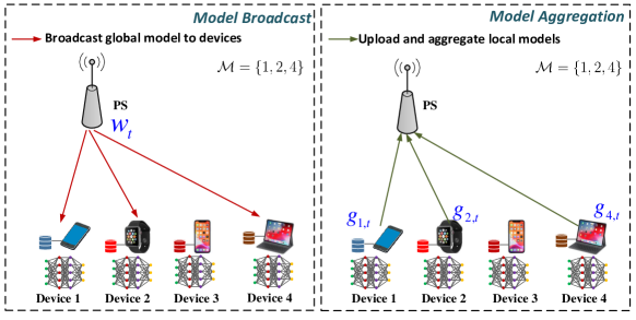
Figure 1: Illustration of the $t$-th FL training round with $M=4$.

To perform FL, the edge devices update their local models by minimizing $F_{m}$, and the PS aggregates the global model based on the local updates. In this paper, we adopt batch gradient descent [BGD] for local model update. Specifically, the model ${\bf w}$ is computed iteratively with $T$ training rounds. The $t$-th round, $1\leq t\leq T$, includes the following procedures:

• Device selection: The PS selects a subset of mobile devices $\mathcal{M}_{t}\subset\{1,2,\cdots,M\}$ to participate in the learning process. We refer to the devices in $\mathcal{M}_{t}$ as the active devices.

• Model broadcast: The PS broadcasts the current global model ${\bf w}_{t}$ to the active devices.

• Local gradient computation: Each active device computes its local gradient with respect to the local dataset. Specifically, the gradient is given by

  $${\bf g}_{m,t}\triangleq\nabla F_{m}({\bf w}_{t};\mathcal{D}_{m})\in\mathbb{R}^{D},$$ (3)

  where $\nabla F_{m}({\bf w}_{t};\mathcal{D}_{m})$ is the gradient of $F_{m}(\cdot)$ at ${\bf w}={\bf w}_{t}$.

• Model aggregation: The active devices upload $\{{\bf g}_{m,t}\}$ to the PS through wireless channels. Based on the received signals, the PS intends to compute a weighted sum of the local gradients $\{{\bf g}_{m,t}:m\in\mathcal{M}_{t}\}$, which is used to update the global model. In this paper, we consider the popular FL setup introduced in [FEDSGD], where the weight of the $m$-th local gradient vector is proportional to the size of the corresponding local dataset $K_{m}$. In this case, we want to estimate ${\bf r}_{t}\triangleq\sum_{m\in\mathcal{M}_{t}}K_{m}{\bf g}_{m,t}$ at the PS from the received signals. We refer to ${\bf r}_{t}$ the (true) global gradient vector, and denote the estimate of ${\bf r}_{t}$ by $\hat{\bf r}_{t}$. Due to channel fading and communication noise, there inevitably exist distortions in the estimation process. Therefore, we generally have $\hat{\bf r}_{t}\neq{\bf r}_{t}$. After obtaining $\hat{\bf r}_{t}$, we update ${\bf w}_{t+1}$ by

  $${\bf w}_{t+1}={\bf w}_{t}-\frac{\lambda}{\sum_{m\in\mathcal{M}_{t}}K_{m}}{\hat{\bf r}_{t}},$$ (4)

  where a scaling factor $1/({\sum_{m\in\mathcal{M}_{t}}K_{m}})$ is introduced [FEDSGD]; and $\lambda$ is the learning rate.

To improve the communication efficiency, we select a subset of the devices to be active by following [FEDSGD]. For simplicity, we assume that the wireless channel is invariant during the learning process. The studies on time-varying channels can be found in Section LABEL:sec6g. Consequently, we fix the device selection for all iterations, i.e., $\mathcal{M}_{t}=\mathcal{M},\forall t$. Note that $\mathcal{M}$ should be jointly optimized with the transceivers by taking into account both the channel heterogeneity (e.g., channel fading varies across the edge devices) and the data heterogeneity (e.g., the devices hold different numbers of training samples).

Remark 1.

There exist many variants of the above gradient descent algorithm. For example, the authors in [FEDSGD] replaced the single gradient ${\bf g}_{m,t}$ in (3) with a sequence of multiple-batch gradient descent updates (a.k.a. federated stochastic gradient descent) and/or multiple-epoch updates (a.k.a. federated averaging). Although the analysis in this paper adopts the model in (3), we show by numerical results in Section LABEL:sec6d that the proposed approach can improve the learning performance of multiple-batch/epoch FL algorithms as well.

II-B RIS-Assisted Communication System

The underlying wireless network for the above FL system is depicted in Fig. 2, where a RIS is deployed to assist the communication between the single-antenna edge devices and the $N$-antenna PS. Suppose that the RIS has $L$ phase shift elements. We assume a block fading channel model, where the channel coefficients remain invariant during the whole FL training process. Let ${\bf h}_{DP,m}\in\mathbb{C}^{N\times 1}$, ${\bf H}_{RP}\in\mathbb{C}^{N\times L}$, and ${\bf h}_{DR,m}\in\mathbb{C}^{L\times 1}$, $m=1,2,\cdots,M$, denote the direct $m$-th-device-PS, the RIS-PS, and the $m$-th-device-RIS channel coefficient vectors/matrix, respectively. We assume perfect channel state information (CSI) at the PS, the RIS controller, and the devices. Thanks to the reconfigurable property of the RIS, the RIS elements induce independent phase shifts on the incident signals. We keep the RIS phase shifts invariant during the FL model aggregation and denote the RIS phase-shift vector as $\bm{\theta}\in\mathbb{C}^{L\times 1}$. We set the RIS amplitude reflection coefficients to $1$ and assume continuous RIS phase shifts with $\lvert\theta_{l}\rvert^{2}=1$ for $l=1,2,\cdots,L$.

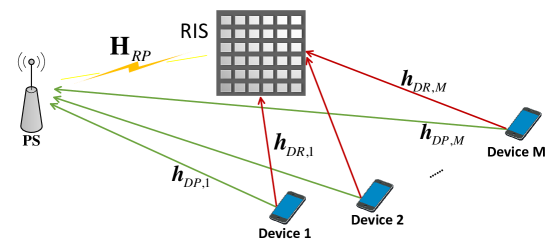
Figure 2: A RIS-assisted communication system.

For ease of notation, we define the effective $m$-th-device-PS channel coefficient vector as

$${\bf h}_{m}(\bm{\theta})\triangleq{\bf h}_{DP,m}+{\bf H}_{RP}\mathop{\rm diag}\nolimits(\bm{\theta}){\bf h}_{DR,m}={\bf h}_{DP,m}+{\bf G}_{m}\bm{\theta},$$ (5)

where ${\bf G}_{m}\triangleq{\bf H}_{RP}\mathop{\rm diag}\nolimits({\bf h}_{DR,m})\in\mathbb{C}^{N\times L}$ is the $m$-th cascaded channel coefficient matrix.

In the model aggregation of the $t$-th training round, we denote the transmit signal from the active devices in time slot $d$ by $\{x_{m,t}[d]:m\in\mathcal{M}\}$. The corresponding received signal at the PS, denoted by ${\bf y}_{t}[d]$, is the superposition of the signals from the direct channels and the device-RIS-PS cascaded channels, i.e.,

$${\bf y}_{t}[d] =\sum_{m\in\mathcal{M}}\left({\bf h}_{DP,m}+{\bf H}_{RP}\mathop{\rm diag}\nolimits(\bm{\theta}){\bf h}_{DR,m}\right)x_{m,t}[d]+{\bf n}_{t}[d]=\sum_{m\in\mathcal{M}}{\bf h}_{m}(\bm{\theta})x_{m,t}[d]+{\bf n}_{t}[d],$$ (6)

where ${\bf n}_{t}[d]\in\mathbb{C}^{N\times 1}$ is an additive white Gaussian noise (AWGN) vector with the entries following the distribution of $\mathcal{CN}(0,\sigma_{n}^{2})$.

II-C Over-the-Air Model Aggregation

We adopt over-the-air computation to achieve FL model aggregation [GZhu_BroadbandAircomp]. Specifically, at the $t$-th training round, $1\leq t\leq T$, the active devices upload their local model updates $\{{\bf g}_{m,t}:m\in\mathcal{M}\}$ using the same time-frequency resources. By controlling the transmit equalization factors, the desired weighted sum $\hat{\bf r}_{t}$ in (4) is coherently constructed at the PS. The details are discussed as follows.

In the sequel, we omit the index $t$ for brevity. Denote the $d$-th entry of ${\bf g}_{m}$ by $g_{m}[d]$. To perform over-the-air model aggregation, $\{g_{m}[d]\}$ are first transferred to $D$-slot transmit signals $\{x_{m}[d]:1\leq d\leq D,m\in\mathcal{M}\}$. Specifically, we first compute the local gradient statistics (i.e., the means and variances) for $\forall m\in\mathcal{M}$ by

$$\bar{g}_{m}=\frac{1}{D}\sum_{d=1}^{D}g_{m}[d],\quad\nu_{m}^{2}=\frac{1}{D}\sum_{d=1}^{D}(g_{m}[d]-\bar{g}_{m})^{2}.$$ (7)

Then, the active devices upload these scalar quantities $\{\bar{g}_{m},\nu_{m}^{2}\}$ to the PS.

The $m$-th device sets the transmit sequence $\{x_{m}[d]:1\leq d\leq D\}$ as

$$x_{m}[d]=p_{m}s_{m}[d]\text{ with }s_{m}[d]\triangleq\frac{g_{m}[d]-\bar{g}_{m}}{\nu_{m}},\forall d,$$ (8)

where $p_{m}\in\mathbb{C}$ is the transmit equalization factor used to combat the channel fading and achieve the desired weight (i.e., $K_{m}$) at the PS. In (8), $g_{m}[d]$ is mapped to a zero-mean unit-variance symbol $s_{m}[d]$ by using $\bar{g}_{m}$ and $\nu_{m}$ such that $\mathbb{E}[s_{m}[d]]=0$ and $\mathbb{E}[s_{m}^{2}[d]]=1$. This normalization step ensures that $\mathbb{E}[\lvert x_{m}[d]\rvert^{2}]=\lvert p_{m}\rvert^{2}$, where $\lvert p_{m}\rvert^{2}$ controls the transmit power. Here, we consider an individual transmit power constraint as

$$\mathbb{E}\left[\lvert x_{m}[d]\rvert^{2}\right]=\lvert p_{m}\rvert^{2}\leq P_{0},\forall m,$$ (9)

where $P_{0}$ is the maximum transmit power.

Substituting (8) into (6), the received signal at the PS in time slot $d$ is given by

$${\bf y}[d] =\sum_{m\in\mathcal{M}}{\bf h}_{m}(\bm{\theta})\frac{p_{m}}{\nu_{m}}(g_{m}[d]-\bar{g}_{m})+{\bf n}[d].$$ (10)

The PS computes the estimate of $r[d]=\sum_{m\in\mathcal{M}}K_{m}g_{m}[d]$, i.e., $\hat{r}[d]$, from ${\bf y}[d]$ by a linear estimator as

$$\hat{r}[d]=\frac{1}{\sqrt{\eta}}{\bf f}^{H}{\bf y}[d]+\bar{g}=\frac{1}{\sqrt{\eta}}\left(\sum_{m\in\mathcal{M}}{\bf f}^{H}{\bf h}_{m}(\bm{\theta})\frac{p_{m}}{\nu_{m}}(g_{m}[d]-\bar{g}_{m})+{\bf f}^{H}{\bf n}[d]\right)+\bar{g},$$ (11)

where $\bar{g}\triangleq\sum_{m\in\mathcal{M}}K_{m}\bar{g}_{m}$; ${\bf f}\in\mathbb{C}^{N\times 1}$ is the normalized receiver beamforming vector with $\lVert{\bf f}\rVert_{2}^{2}=1$; and $\eta>0$ is a normalization scalar. In (11), we add an additional term $\bar{g}=\sum_{m}K_{m}\bar{g}_{m}$ that is related to the local means $\{\bar{g}_{m}\}$ since $\bar{g}_{m}$ has been subtracted in the normalization step in (8).

After estimating $\hat{\bf r}=[\hat{r}[1],\cdots,\hat{r}[D]]$, we update the global model by (4). Note that the existences of fading and communication noise lead to inevitable estimation error in $\hat{\bf r}$. As a result, the global model update in (4) becomes inaccurate, which affects the convergence of FL. In the next section, we quantitatively characterize the impact of the communication error on the convergence of FL with respect to $\{\mathcal{M},{\bf f},\bm{\theta},\eta,p_{m}\}$.

Remark 2.

We note that the proposed over-the-air model aggregation framework is different from the existing solutions [FL_2, FL_1, GZhu_BroadbandAircomp] in the following two aspects:

• Refs. [FL_2, FL_1] only assume that $g_{m}[d]$ is mapped to $s_{m}[d]$ without discussing the details on the normalization method. Besides, Ref. [GZhu_BroadbandAircomp] sets $s_{m}[d]={(g_{m}[d]-\bar{g})}/{\nu}$, where $\bar{g}$ is defined in (11) and $\nu^{2}\triangleq\sum_{m\in\mathcal{M}}K_{m}\nu^{2}_{m}$. In other words, two uniform statistics $\bar{g}$ and $\nu^{2}$ are used to compute $s_{m}[d]$ for $\forall m$. When the local gradients $\{{\bf g}_{m}\}$ significantly vary among the active devices, this normalization cannot guarantee $\mathbb{E}[s_{m}^{2}[d]]=1$ for $\forall m$, and hence the constraint in (9) may become unsatisfied. In contrast, we normalize the transmit signal by the local gradient statistics, ensuring that (9) always holds.

• Refs. [FL_2, FL_1, GZhu_BroadbandAircomp] measure the over-the-air model aggregation performance by the estimation error with respect to $\sum_{m\in\mathcal{M}}K_{m}s_{m}[d]$ rather than that of $\sum_{m\in\mathcal{M}}K_{m}g_{m}[d]$. In contrast, we directly consider the estimation on $\hat{r}[d]$ in (11) by explicitly taking the de-normalization step into account. By doing so, we can model the impact of the whole model aggregation process on the learning performance as detailed in Section III.

III FL Performance Analysis and Problem Formulation

In this section, we analyze the performance of the FL task under the over-the-air model aggregation framework. In Section III-A, we introduce several assumptions on the loss function $F(\cdot)$. Based on these assumptions, we derive a tractable upper bound on the learning loss $F({\bf w}_{t})$ by analyzing the model updating error caused by the device selection and the communication noise. Then, we give a closed-form solution to $\{\eta,p_{m},\forall m\}$ that minimizes the loss bound. Finally, we formulate the system design problem as a unified learning loss minimization task over the device selection decision $\mathcal{M}$, the receiver beamforming vector ${\bf f}$, and the RIS phase shift vector $\bm{\theta}$.

III-A Assumptions and Preliminaries

Recall that the PS computes $\hat{\bf r}_{t}$ by the over-the-air model aggregation in (11). Consequently, the global model update recursion is given by

$${\bf w}_{t+1}={\bf w}_{t}-\frac{\lambda}{\sum_{m\in\mathcal{M}}K_{m}}\hat{\bf r}_{t}={\bf w}_{t}-\lambda(\nabla F({\bf w}_{t})-{\bf e}_{t}),$$ (12)

where $\nabla F({\bf w}_{t})\triangleq\frac{1}{K}\sum_{k=1}^{K}\nabla f({\bf w}_{t};{\bf x}_{k},y_{k})$ is the gradient of $F({\bf w})$ at ${\bf w}={\bf w}_{t}$; and ${\bf e}_{t}$ denotes the gradient error vector due to the device selection and model aggregation. Specifically, ${\bf e}_{t}$ is given by

$${\bf e}_{t}= \underbrace{\nabla F({\bf w}_{t})-\frac{{\bf r}_{t}}{\sum_{m\in\mathcal{M}}K_{m}}}_{{\bf e}_{1,t}\text{(error due to device selection)}}+\underbrace{\frac{{\bf r}_{t}}{\sum_{m\in\mathcal{M}}K_{m}}-\frac{\hat{\bf r}_{t}}{\sum_{m\in\mathcal{M}}K_{m}}}_{{\bf e}_{2,t}\text{(error due to fading and communication noise)}}.$$ (13)

From (13), we see that ${\bf e}_{1,t}=\bf 0$ if $\mathcal{M}=\{1,2,\cdots,M\}$ and ${\bf e}_{1,t}\neq\bf 0$ if $|\mathcal{M}|<M$. Intuitively, device selection reduces the amount of exploited data and induces additional error ${\bf e}_{1,t}$ on the gradient vector $\nabla F({\bf w}_{t})$. As shown later in this section, this error, together with the error in model aggregation (i.e., ${\bf e}_{2,t}$), jointly jeopardizes the performance of FL.

To proceed, we make the following assumptions on the loss function $F(\cdot)$:

A1

$F$ is strongly convex with parameter $\mu$. That is, $F({\bf w})\geq F({\bf w}^{\prime})+({\bf w}-{\bf w}^{\prime})^{T}\nabla F({\bf w}^{\prime})+\frac{\mu}{2}\lVert{\bf w}-{\bf w}^{\prime}\rVert_{2}^{2},\forall{\bf w},{\bf w}^{\prime}\in\mathbb{R}^{D\times 1}$.

A2

The gradient $\nabla F(\cdot)$ is Lipschitz continuous with parameter $\omega$. That is, $\lVert\nabla F({\bf w})-\nabla F({\bf w}^{\prime})\rVert_{2}\leq\omega\lVert{\bf w}-{\bf w}^{\prime}\rVert_{2},\forall{\bf w},{\bf w}^{\prime}\in\mathbb{R}^{D\times 1}$.

A3

$F$ is twice-continuously differentiable.

A4

The gradient with respect to any training sample, $\nabla f(\cdot)$, is upper bounded at $\{{\bf w}_{t}:\forall 1\leq t\leq T\}$. That is,

$$\lVert\nabla f({\bf w}_{t};{\bf x}_{k},y_{k})\rVert_{2}^{2}\leq\alpha_{1}+\alpha_{2}\lVert\nabla F({\bf w}_{t})\rVert_{2}^{2},\forall 1\leq k\leq K,\forall 1\leq t\leq T,$$ (14)

for some constants $\alpha_{1}\geq 0$ and $\alpha_{2}>0$.

Assumptions A1–A4 are standard in the stochastic optimization literature; see, e.g., [NDP, Friedlander2012, chen2019joint]. Assumption A1 ensures that a global optimum ${\bf w}^{\star}$ exists for the loss function $F$. Assumption A4 provides a bound on the norm of the local gradient vectors. Note that the parameter $\alpha_{1}$ allows the local gradient to be nonzero even if the global gradient is zero. In practice, Assumptions A1-A3 hold for many regularized problems; see, e.g., [Friedlander2012, Section 5]. Concerning A4, it is reasonable to expect that $K,T<\infty$ and $\lVert\nabla f({\bf w}_{t};\cdot)\rVert_{2}^{2}<\infty$ in practice. In this case, we can exhaustively check the values of $\{\lVert\nabla f({\bf w}_{t};{\bf x}_{k},y_{k})\rVert_{2}^{2}\}_{k=1}^{K}$ over $\{{\bf w}_{t}\}_{t=1}^{T}$ to find sufficiently large $\alpha_{1}$ and $\alpha_{2}$ such that A4 holds.

As shown in [Friedlander2012, Lemma 2.1], Assumptions A1–A4 lead to an upper bound on the loss function $F({\bf w}_{t+1})$ with respect to the recursion (12) with a proper choice of the learning rate $\lambda$. The details are given in the following lemma.

Lemma 1.

Suppose that $F(\cdot)$ satisfies Assumptions A1–A4. At the $t$-th training round, with $\lambda=1/\omega$, we have

$$\mathbb{E}[F({\bf w}_{t+1})]\leq\mathbb{E}[F({\bf w}_{t})]-\frac{1}{2\omega}\lVert\nabla F({\bf w}_{t})\rVert_{2}^{2}+\frac{1}{2\omega}\mathbb{E}[\lVert{\bf e}_{t}\rVert_{2}^{2}],$$ (15)

where the Lipschitz constant $\omega$ is defined in Assumption A2, and the expectations are taken with respect to the communication noise.

Proof.

See [Friedlander2012, Lemma 2.1].

III-B Learning Performance Analysis

With Assumptions A1–A4 and Lemma 1, we are ready to present the performance analysis. Specifically, we apply Lemma 1 and bound the term $\mathbb{E}[\lVert{\bf e}_{t}\rVert^{2}]$ to derive a tractable expression of $\mathbb{E}[F({\bf w}_{t+1})]$. This expression is further used to obtain an upper bound of the average difference between the training loss and the optimal loss, i.e., $\mathbb{E}\left[F({\bf w}_{t+1})-F({\bf w}^{\star})\right]$.

To begin with, we apply Lemma 1 and obtain

$$\mathbb{E}[F({\bf w}_{t+1})] \leq\mathbb{E}[F({\bf w}_{t})]-\frac{1}{2\omega}\lVert\nabla F({\bf w}_{t})\rVert_{2}^{2}+\frac{1}{2\omega}\mathbb{E}[\lVert{\bf e}_{1,t}+{\bf e}_{2,t}\rVert_{2}^{2}]$$

$$\overset{(a)}{\leq}\mathbb{E}[F({\bf w}_{t})]-\frac{1}{2\omega}\lVert\nabla F({\bf w}_{t})\rVert_{2}^{2}+\frac{1}{2\omega}\mathbb{E}\left[(\lVert{\bf e}_{1,t}\rVert_{2}+\lVert{\bf e}_{2,t}\rVert_{2})^{2}\right]$$

$$\overset{(b)}{\leq}E[F({\bf w}_{t})]-\frac{1}{2\omega}\lVert\nabla F({\bf w}_{t})\rVert_{2}^{2}+\frac{1}{\omega}(\lVert{\bf e}_{1,t}\rVert^{2}_{2}+\mathbb{E}\left[\lVert{\bf e}_{2,t}\rVert^{2}_{2}\right])$$ (16)

where the expectations are taken with respect to the communication noise; $(a)$ is from the triangle inequality; and $(b)$ is from the inequality of arithmetic and geometric means (AM–GM inequality). In the last step of (III-B), we drop the expectation on $\lVert{\bf e}_{1,t}\rVert^{2}_{2}$ since ${\bf e}_{1,t}$ is independent to the communication noise.

To analyze $\mathbb{E}[F({\bf w}_{t+1})]$, we need tractable expressions for $\lVert{\bf e}_{1,t}\rVert_{2}^{2}/\omega$ and $\mathbb{E}[\lVert{\bf e}_{2,t}\rVert_{2}^{2}]/\omega$. Note that the error ${\bf e}_{1,t}$ is determined by the device selection decision $\mathcal{M}$, whereas the communication error ${\bf e}_{2,t}$ is related to $\mathcal{M}$ and $\{{\bf f},\bm{\theta},\eta,p_{m},\forall m\in\mathcal{M}\}$. For given $\mathcal{M}$, the choice of $\{\eta,p_{m},\forall m\}$ that minimizes $\mathbb{E}[\lVert{\bf e}_{2,t}\rVert_{2}^{2}]$ is given in the following lemma.

Lemma 2.

Under the transmit power constraint (9), the optimal $\{\eta,p_{m}\}$ that minimizes $\mathbb{E}[\lVert{\bf e}_{2,t}\rVert_{2}^{2}]$ is given by

$$\eta=\min_{m\in\mathcal{M}}\frac{P_{0}\lvert{\bf f}^{H}{\bf h}_{m}(\bm{\theta})\rvert^{2}}{K_{m}^{2}\nu_{m}^{2}},p_{m}=\frac{K_{m}\sqrt{\eta}\nu_{m}({\bf f}^{H}{\bf h}_{m}(\bm{\theta}))^{H}}{\lvert{\bf f}^{H}{\bf h}_{m}(\bm{\theta})\rvert^{2}}.$$ (17)

Moreover, $\mathbb{E}[\lVert{\bf e}_{2,t}\rVert_{2}^{2}]$ (as a function of $\mathcal{M}$, $\bm{\theta}$, and ${\bf f}$) with (17) is given by

$$\mathbb{E}[\lVert{\bf e}_{2,t}\rVert_{2}^{2}]=\frac{D\sigma^{2}_{n}}{P_{0}\left(\sum_{m\in\mathcal{M}}K_{m}\right)^{2}}\max_{m\in\mathcal{M}}\frac{K_{m}^{2}\nu_{m}^{2}}{\lvert{\bf f}^{H}{\bf h}_{m}(\bm{\theta})\rvert^{2}}.$$ (18)

Proof.

See Appendix LABEL:appa0.

Lemma 2 gives the optimal solution to $\{\eta,p_{m},\forall m\}$ and the corresponding expression of $\mathbb{E}[\lVert{\bf e}_{2,t}\rVert_{2}^{2}]$. Based on Lemma 2, we bound $\mathbb{E}\left[F({\bf w}_{t+1})-F({\bf w}^{\star})\right]$ for given $\{\mathcal{M}$, ${\bf f}$, $\bm{\theta}\}$ in the following theorem.