Novel approach for the study of coherent elastic neutrino-nucleus scattering

Abstract

We propose the use of isotopically highly enriched detectors for the precise study of coherent-elastic neutrino-nucleus scattering (CEvNS). CEvNS has been measured for the first time in CsI and recently confirmed with a liquid argon detector. It is expected that several new experimental setups will measure this process with increasing accuracy. Taking Ge detectors as a working example, we demonstrate that a combination of different isotopes is an excellent option to do precision neutrino physics with CEvNS, test Standard Model predictions, and probe new physics scenarios. Experiments based on this new idea can make simultaneous differential CEvNS measurements with detectors of different isotopic composition. Particular combination of observables could be used to cancel systematic errors. While many applications are possible, we illustrate the idea with three examples: testing the dominant quadratic dependence on the number of neutrons, $N$, that is predicted by the theoretical models; constraining the average neutron root mean square (rms) radius; and testing the weak mixing angle and the sensitivity to new physics. In all three cases we find that the extra sensitivity provided by this method will potentially allow high-precision robust measurements with CEvNS and particularly, will resolve the characteristic degeneracies appearing in new physics scenarios.

I Introduction

Neutrinos in the energy region (1 MeV $\leq$ $E_{\nu}$ $\leq$ 50 MeV) such as those generated in reactors or pion decay-at-rest sources ($\pi$-DAR), provide a new means of testing the Standard Model (SM) and its possible extensions. Precise measurements are required to understand the nature of the neutrino, to elucidate the phenomena that give rise to its unique properties and to determine its impact on the evolution of the Universe. After more than forty years of being proposed Freedman:1973yd , the coherent elastic neutrino nucleus-scattering (CEvNS) was observed for the first time in 2017 by the COHERENT collaboration Akimov:2017ade ; Akimov:2018vzs through a CsI detector located at the Spallation Neutron Source (SNS) at Oak Ridge National Laboratory (ORNL). This process has also been confirmed by the same collaboration by using a liquid argon detector Akimov:2019rhz ; Akimov:2020pdx .

A precise measurement of CEvNS is of interest for many fields such as nuclear physics, particle physics, and applications. Just to mention some examples, CEvNS can help to extract detailed information about the nuclear radius for different target materials Cadeddu:2017etk ; Papoulias:2019lfi ; AristizabalSierra:2019zmy ; Coloma:2020nhf , form factors Hoferichter:2020osn , precision physics Tomalak:2020zfh as well as to constrain parameters which describe physics beyond the SM such as non-standard interactions Barranco:2005yy ; Scholberg:2005qs ; Billard:2018jnl , light mediators Farzan:2018gtr , neutrino magnetic moments Wong:2003xj ; Miranda:2019wdy or sterile neutrinos Dutta:2015nlo ; Canas:2017umu ; Miranda:2020syh . An application of considerable interest of reactor antineutrino detection using CEvNS is in nuclear security Bowen:2020unj .

We propose a novel approach for the precise study of CEvNS; namely, the use of isotopically highly enriched detectors. We discuss Ge as a concrete example to show feasibility, but the proposed technique of using isotopically enriched material has much more general applicability. A detector array based on multi-isotope detectors would have a particular combination of observables providing a fast unambiguous signature of antineutrino detection.

It was noticed, since the first theoretical proposal of CEvNS by Freedman Freedman:1973yd , that its corresponding cross section has a quadratic dependence on the number of neutrons due to its coherent character. This enhancement makes the process very attractive both experimentally and theoretically Barranco:2005yy . The large cross section makes it the dominant process at low energies and opens a new detection channel that can give new independent physical information. Despite this advantage, the heavy mass of the nucleus implies the detection of a very low energy recoil and makes the measurement an experimental challenge. Nuclear recoil signals at low energies are not well calibrated and the ability to observe CEvNS from a reactor flux is very dependent on low-energy quenching factors (QF). These are not well known and their uncertainties are considerable. Significant progress has been made recently to better understand the associated systematic effects Collar:2019ihs ; Collar:2021fcl . An example is the dramatic reduction of uncertainties on the QF’s for CsI from 25% in 2017 (first observation of CEvNS) to less than 5% in 2021 Tayloe . Long experiments might require corrections due to small drifts or for nonlinearities in the signal digitizer. Besides, as the process is testing a new energy region, it is natural that theoretical uncertainties will appear. That is the case, for instance, of the mean neutron radius of the target nuclei, for which, usually, only theoretical predictions exist. As a first step to test physics beyond the SM, the variables under discussion have to be well determined.

In this concept paper we propose a general experimental method to improve the CEvNS accuracy by using an array of detectors of the same element but different isotopes. The use of such an array will help to diminish systematic errors (from flux uncertainties, for instance) and to mitigate the dependence on form factors (FF), allowing a better knowledge of the cross section and making it an even better tool for testing new physics. Currently, there are several proposals either ongoing or planned to measure CEvNS with a stopped-pion neutrino source or with reactor antineutrinos using different target materials. For example, CONNIE using Si-based CCDs Aguilar-Arevalo:2016qen ; Aguilar-Arevalo:2019jlr ; COHERENT Akimov:2018ghi , CONUS Lindner:2016wff , $\nu$GEN Belov_2015 , and TEXONO Wong:2005vg , using ionization-based Ge semiconductors; and MINER Agnolet:2016zir , NuCLEUS Angloher:2019flc , and RICOCHET Billard:2016giu using cryogenic detectors (Si, Zn, Ge). The proposed technique discussed here could be applied to any of these technologies, but to illustrate the idea, we will only consider the germanium case. The process of isotopically enriching germanium is a well-developed technology that has provided highly-enriched ⁷⁶Ge for detectors used in the search for neutrinoless double beta decay Gunther:1997ai ; Gradwohl:2020kms . Furthermore, isotopically modified Ge detectors depleted in ⁷⁶Ge have been produced and showed identical performance as those produced previously from natural germanium material Budjas:2013bea ; Agostini:2012ifa . Mitigation or cancelation of the effect of systematic uncertainties is a crucial issue in many fields of Physics. The high isotopic purity of 90 $\%$ or better that can be achieved in the detector materials (e.g. Ge) and the possibility of producing identical detectors that differ only in the number of neutrons provides a unique laboratory for the study of the CEvNS interaction.

We present how such an array of Ge detectors could test and constrain different parameters involving nuclear and particle physics. In section II, we study the $N^{2}$ CEvNS dependence. We study the sensitivity in determining of the nuclear rms radius on section III, which is relevant for the characterization of DM detectors. We discuss in section IV the expected constraints for the weak mixing angle at low energies and Non-Standard Interactions (NSI) parameters. In all the cases, we show the impact of the correlation between systematic uncertainties on the determination of these observables. We focus our discussion on these examples, but it is important to remark that there is a wide margin to drastically improve other observables with this experimental approach.

Furthermore, it will be shown that the differential nuclear recoil spectra have a non-trivial relative shape between the different isotopes. Its understanding will also help to inform the $N$ dependence of CEvNS and other observables, by conveniently choosing the appropriate region of energy. We will show that this setup of different germanium detectors can probe this rule. As with any CEvNS experiment, these measurements are inevitably affected by systematic uncertainties that mainly result from quenching and form factors. However, in this particular case, the system of coupled detectors shares the same systematic effects and the correlations help to make a cleaner statement about the relative value of the cross sections.

Within the SM, the explicit form of the CEvNS cross section is

$$\left(\frac{d\sigma}{dT}\right)_{\rm SM}^{\rm coh}=\frac{G_{F}^{2}M}{\pi}\left[1-\frac{MT}{2E_{\nu}^{2}}\right][Zg^{p}_{V}F_{Z}(q^{2})+Ng^{n}_{V}F_{N}(q^{2})]^{2}$$ (1)

with $M$ the mass of the nucleus, $E_{\nu}$ the incident neutrino energy, and $F_{X}$ the nuclear form factors, with $X=Z,N$ for protons and neutrons, respectively. The factors $g_{V}^{p}=1/2-2\sin^{2}\theta_{W}$ and $g_{V}^{n}=1/2$ are the weak coupling constants. Notice that $g_{V}^{p}<<g_{V}^{n}$ and, in consequence, the main dependence in this formula goes as $N^{2}$.

A precise confirmation, for instance, of the $N^{2}$ dependence is challenging. The uncertainties coming from very different detectors with different exposure to the flux makes this task non-trivial. As we show, the use of multiple enriched detectors under simultaneous exposure time, would solve the issue of dealing with different systematic uncertainties. Indeed, for elements with multiple isotopes, the $N^{2}$ dependence of CEvNS can provide a significant variation in the measured number of events for each nuclei. In particular, for germanium ($Z=$ 32) we have five stable natural isotopes: ⁷⁰Ge, ⁷²Ge, ⁷³Ge, ⁷⁴Ge, and ⁷⁶Ge, implying a difference of up to $15$ % in the relative number of neutrons.

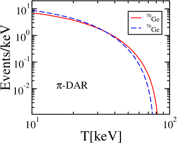
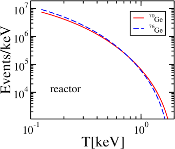
Figure 1: Differential event rate in terms of the nuclear recoil for two different isotopes (⁷⁰Ge and ⁷⁶Ge) exposed to a stopped-pion neutrino source (left) or a reactor flux (right). As discussed in the text, we can see that for higher energies the lighter ⁷⁰Ge has higher predicted rates per keV in both cases.

It is important to notice the behavior of the nuclear recoil energy spectra due to the neutron number. We would expect that the main difference between any two isotopes should be dominated by the variation between the squares of the corresponding number of neutrons for each isotope. However, the different masses of the isotopes also play an important role, especially at the high energy tail of the recoil energy spectrum. We can illustrate this by considering two different isotopes, having $N_{1}$ and $N_{2}$ neutrons and a mass given approximately by $(Z+N_{i})m_{N}$ with $m_{N}$ the mass of an average nucleon. Taking only leading terms, the difference between their cross sections will be, approximately,

$$\delta=\frac{d\sigma(N_{2})}{dT}-\frac{d\sigma(N_{1})}{dT}=\frac{G_{F}m_{N}}{\pi}\left(a(N_{1},N_{2},Z)-b(N_{1},N_{2},Z)\frac{m_{N}T}{2E^{2}_{\nu}}\right)$$ (2)

with

$$a(N_{1},N_{2},Z) = {g^{n}_{V}}^{2}\left(Z(N^{2}_{2}-N^{2}_{1})+(N^{3}_{2}-N^{3}_{1})\right)$$

$$b(N_{1},N_{2},Z) = {g^{n}_{V}}^{2}\left(Z^{2}(N^{2}_{2}-N^{2}_{1})+2Z(N^{3}_{2}-N^{3}_{1})+(N^{4}_{2}-N^{4}_{1})\right).$$ (3)

For the case of ⁷⁰Ge and ⁷⁶Ge, we will have $a/b\simeq 0.01$, which means that the difference, $\delta$, will vanish for $T=0.02E^{2}_{\nu}/m_{N}$. For example for a reactor antineutrino of $E_{\nu}$ = 6 MeV this happens around $T\approx 0.7$ keV, while for a $\pi$-DAR source for a neutrino of $E_{\nu}$ = 40 MeV, the same situation arises at $T\approx 32$ keV. The more appealing result is that $\delta$ will be negative for recoil energies above these values, that is, despite our expectation of a higher number of events for heavier isotopes, this is not the case in the tail of the recoil spectrum, an odd feature that could help to test the predicted CEvNS cross section. This is illustrated in Fig. 1 for reactor and $\pi$-DAR neutrinos, where we show the expected differential rate for two different isotopes after integrating over the incoming neutrino energy in each case.

In general, to study the response of the proposed array of isotopically enriched detectors, we start by defining the expected number of events, given by the convolution of the differential cross section, $d\sigma/dT$, and the neutrino flux, $\phi(E)$, that is:

$$\mathcal{N}^{theo}=N_{D}\int_{T}A(T)dT\int_{E_{min}}^{E_{Max}}dE\phi(E)\frac{\mathrm{d}\sigma}{\mathrm{d}T},$$ (4)

with $N_{D}$ the effective number of target nuclei within the detector during the running time of the experiment, and $A(T)$ an acceptance function.

We can use the total number of events predicted by Eq. (4) to perform different tests. In general, given a set of different detectors for which correlations are present, we can use a simple $\chi^{2}$ analysis by minimizing the function:

$$\chi^{2}=\sum_{ij}(\mathcal{N}_{i}^{theo}-\mathcal{N}_{i}^{exp})[\sigma_{ij}^{2}]^{-1}(\mathcal{N}_{j}^{theo}-\mathcal{N}_{j}^{exp}),$$ (5)

where $\sigma_{ij}^{2}$ is the covariant matrix and $\mathcal{N}_{i}^{exp}$ the ‘experimental’ measurement, which we will take as the SM prediction in each case. The theoretical number of events, $\mathcal{N}^{th}_{i}$, depends on the set of parameters under study, and the indices $i$, $j$ run over the number of detectors within the array.

To illustrate the idea, we can consider an experimental array of three different germanium isotopes: ^ℓGe, ^mGe, and ⁿGe (with $\ell$, $m$, and $n$ the total number of nucleons), located at the same distance from the neutrino source and taking data simultaneously. Under these conditions, the detectors will be exposed to the same neutrino flux, regardless of any variations through the running time, and there will be correlations among the systematic uncertainties which, as we will see, will be useful to test the observable under study. This approach can easily be extended to more isotopes and different materials. In our particular example, the covariance matrix is a $3\times 3$ matrix with nonzero elements outside the diagonal due to the correlation between the detectors. Denoting by $A$ and $B$ the most significant sources of errors within the experiment, with $\sigma^{A}_{k}$ and $\sigma^{B}_{k}$ ($k=\ell,m,n$) their corresponding uncertainties for each isotope, we have:

$$\sigma^{2}=\begin{pmatrix}{\sigma_{\ell}^{stat}}^{2}+{\sigma_{\ell}^{A}}^{2}+{\sigma_{\ell}^{B}}^{2}&\sigma_{\ell}^{A}\sigma_{m}^{A}+\sigma_{\ell}^{B}\sigma_{m}^{B}&\sigma_{\ell}^{A}\sigma_{n}^{A}+\sigma_{\ell}^{B}\sigma_{n}^{B}\\ \sigma_{\ell}^{A}\sigma_{m}^{A}+\sigma_{\ell}^{B}\sigma_{m}^{B}&{\sigma_{m}^{stat}}^{2}+{\sigma_{m}^{A}}^{2}+{\sigma_{m}^{B}}^{2}&\sigma_{m}^{A}\sigma_{n}^{A}+\sigma_{m}^{B}\sigma_{n}^{B}\\ \sigma_{\ell}^{A}\sigma_{n}^{A}+\sigma_{\ell}^{B}\sigma_{n}^{B}&\sigma_{m}^{A}\sigma_{n}^{A}+\sigma_{m}^{B}\sigma_{n}^{B}&{\sigma_{n}^{stat}}^{2}+{\sigma_{n}^{A}}^{2}+{\sigma_{n}^{B}}^{2}\end{pmatrix}.$$ (6)

This notation allows us to generalize the matrix elements for experiments with different neutrino sources and detection technologies. The superscript in each case denotes the systematic uncertainty source, while the sub-index makes reference to the associated isotope. In what follows, we will show how this particular approach can be used to study different parameters regarding nuclear and particle physics.

II Testing the $N^{2}$ dependence of CEvNS

The dominance of the CEvNS cross-section, when compared to other processes, comes from the characteristic $N^{2}$ dependence. Here we show some predictions consistent with this dependence when comparing the relative measurements between detectors that differ only in the number of neutrons. To do so, we replace the $N$ factor in Eq. (1) by a variable, $N^{\prime}$, which will test how much an experimental measurement deviates from the $N^{2}$ dependence. Just as the number of neutrons, this factor will be different for each nucleus, and we can express the predicted number of events for a particular detector as:

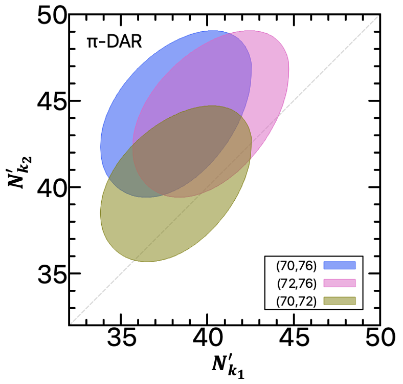
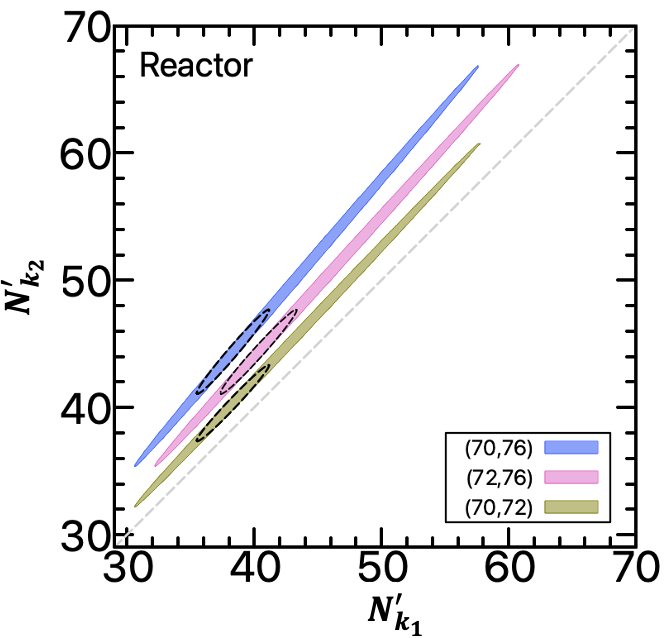
Figure 2: Left panel: Expected measurement of the $N$ dependence in the case of different Germanium detectors within the same experimental setup. We assume that the three detectors, with equal mass, will be exposed to the same $\pi$-DAR neutrino beam with equal contribution of $\sigma_{k}^{A}=$ $\sigma_{k}^{B}=$ 5% from the main systematic errors (see the text for details), that the systematic errors will be correlated, and we consider events from $5$ to $30$ keV nuclear recoil. We show the allowed regions for $N^{\prime}$ values by pairs of isotopes with total nucleons ($k_{1},k_{2}$).The green, magenta and blue regions correspond, respectively, to the results of ⁷⁰Ge vs ⁷²Ge, ⁷²Ge vs ⁷⁶Ge and ⁷⁰Ge vs ⁷⁶Ge at a $90$ % C.L. when marginalizing over the missing detector. The first number in the ordered pair on the inset corresponds to the horizontal axis and the second to the vertical axis. Right panel: We show for comparison the case of a reactor based experiment with an electron recoil energy from 1 to 2 keV. Here we explicitly show the comparison of the results for different systematic uncertainties assumptions. Colored regions refer to the pessimistic case of $\sigma_{k}^{A}=$ 25% and $\sigma_{k}^{B}=$ 10% main systematic contributions. Dashed contours refer to the case of 5% equal contributions.

$$\mathcal{N}^{theo} =N^{\prime 2}\left(g^{n^{2}}_{V}N_{D}\frac{G_{F}^{2}M}{\pi}\int_{T}A(T)dT\int_{E_{min}}^{E_{Max}}dE\left[1-\frac{MT}{2E_{\nu}^{2}}\right]\phi(E)F_{N}^{2}(q^{2})\right)$$ (7)

$$+N^{\prime}\left(Zg^{p}_{V}g^{n}_{V}N_{D}\frac{G_{F}^{2}M}{\pi}\int_{T}A(T)dT\int_{E_{min}}^{E_{Max}}dE\left[1-\frac{MT}{2E_{\nu}^{2}}\right]\phi(E)F_{Z}(q^{2})F_{N}(q^{2})\right)$$

$$+Z^{2}g^{p^{2}}_{V}N_{D}\frac{G_{F}^{2}M}{\pi}\int_{T}A(T)dT\int_{E_{min}}^{E_{Max}}dE\left[1-\frac{MT}{2E_{\nu}^{2}}\right]\phi(E)F_{Z}^{2}(q^{2})$$

The first term in Eq. (7) explicitly shows the dominant quadratic dependence on the number of neutrons for $N^{\prime}=N$. An $N^{2}$ rule would be absolute if $g^{p}_{V}<<g^{n}_{V}$ so that the second and third terms would be negligible. Indeed, this is close to the real case since $g^{p}_{V}/g^{n}_{V}\approx 0.05$; nevertheless, in all our computations we consider the complete expression of Eq. (7). We have explicitly checked that our results for the limiting case $g^{p}_{V}\to 0$ are qualitatively similar. To test the sensitivity to the $N^{2}$ rule we can perform a $\chi^{2}$ analysis following the covariant matrix approach introduced in the previous section, where the parameters under study will be the $N^{\prime}_{k}$ factors, where the sub index $k$ has been introduced to remark that $N^{\prime}$ is different for each isotope. In all our computations we will assume an array of the three different isotopes: ⁷⁰Ge, ⁷²Ge, and ⁷⁶Ge, so we take $\ell=70$, $m=72$, and $n=76$ in Eq. (6). Other combinations can be taken among all of the stable isotopes of germanium. Regarding systematic uncertainties, for $\pi$-DAR neutrinos we take the most significant contributions for systematic uncertainties as those coming from quenching factors ($A$ = QF) and form factors ($B$ = FF). Furthermore we consider two scenarios, one where these contributions are of $\sigma_{k}^{A}=$ 25% and $\sigma_{k}^{B}=$ 10%, respectively, and another scenario where both contributions are of 5%. For reactor sources, we take the main sources of systematic uncertainties as those coming from the quenching factor ($A$ = QF), and the neutrino flux itself ($B$ = NF), with the same numerical configurations as in the case of $\pi$-DAR sources. In addition, for all our computations we consider background effects by adding a 10% contribution of the SM prediction to the statistical uncertainty.

We consider now a neutrino flux from a stopped-pion neutrino source; specifically one with similar characteristics to the SNS at ORNL Akimov:2015nza . In such case, the total incident neutrino flux is given by three different contributions which result from the decay of pions and muons. To calculate the expected number of events, we consider a mass of 10 kg for each isotope, a time of exposure of one year, a Helm distribution for protons and neutrons, and an acceptance function equal to a step function.

The $\chi^{2}$ function in Eq. (5) is a three variable function that defines a volume in the parameter space $N^{\prime}_{k}$ for the allowed values of these factors which are consistent with the theory at a desired C.L.. Three projections are shown in the left panel of Fig. (2) at a 90% C.L. for the configuration where both systematic uncertainties contribute with a 5%. For instance, the magenta region shows the simultaneously allowed $N^{\prime}_{k}$ values for ⁷²Ge and ⁷⁶Ge when marginalizing the information about ⁷⁰Ge. As we can see, the expected region forms an ellipse that restricts the values of $N^{\prime}_{k}$ to lie in correlation to one another according to the $N^{2}$ rule. A similar analysis is shown in green for the pair ⁷⁰Ge, ⁷²Ge and in blue for the pair ⁷⁰Ge, ⁷⁶Ge. Notice that the centroid of the regions are separated from the diagonal, in proportion to the difference in neutron number, as expected.

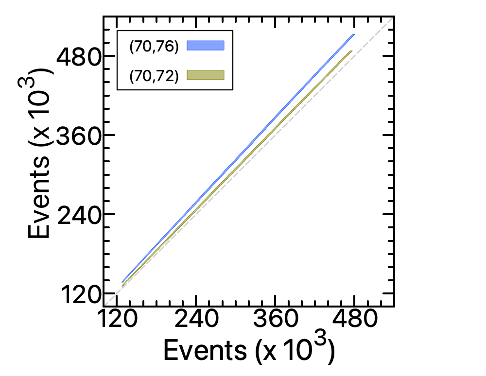
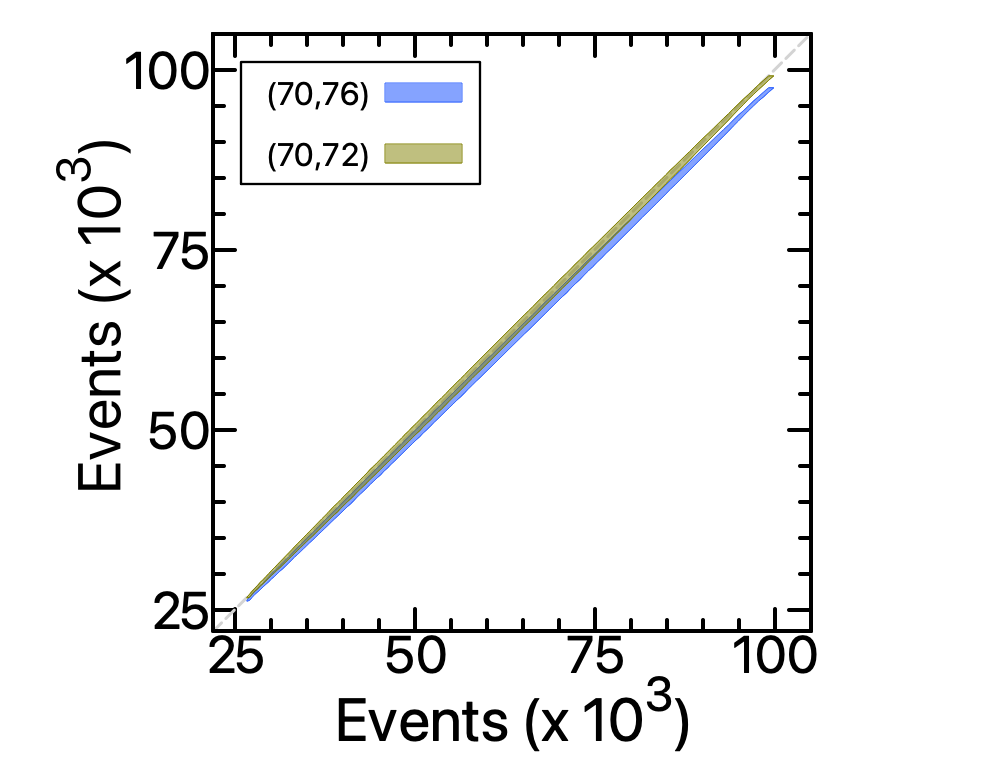
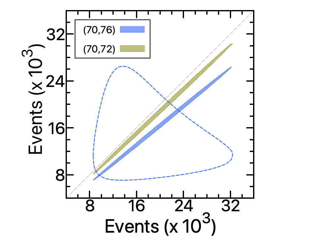
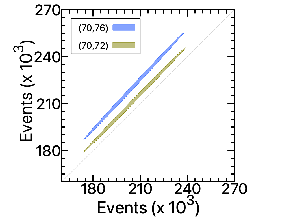
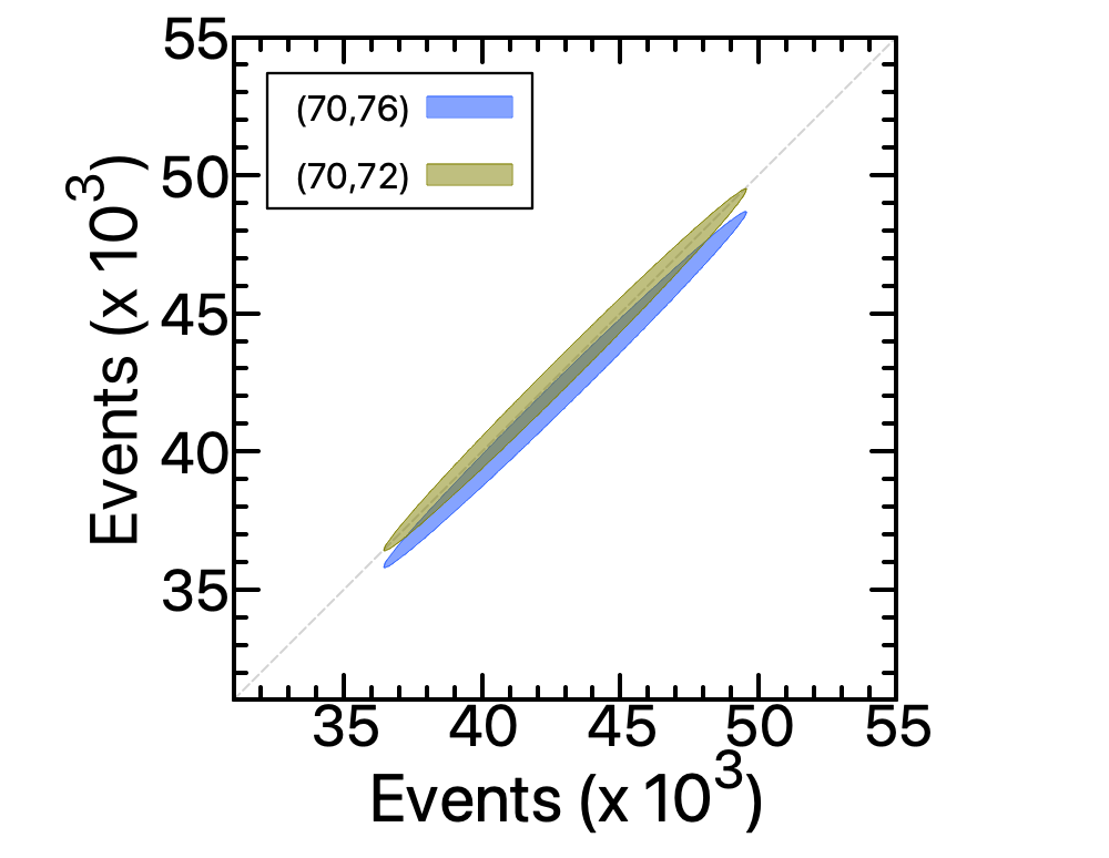
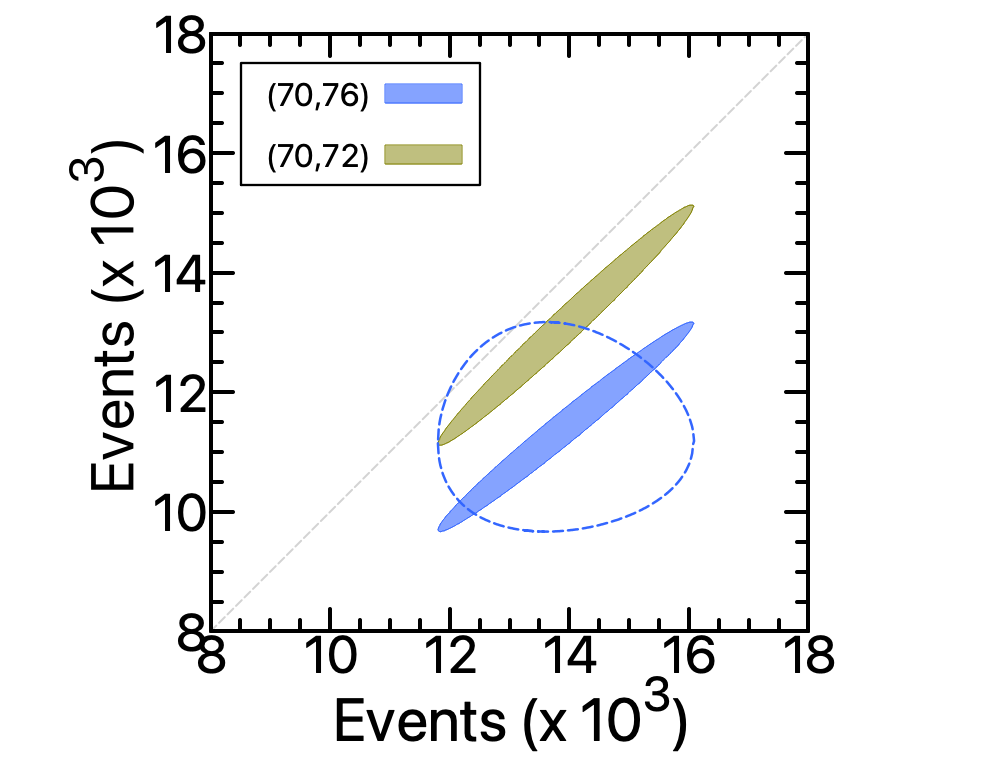
Figure 3: Expected number of events for the three different Ge detectors exposed to a reactor antineutrino flux. The rate from the higher-mass of the two isotopes is shown on the vertical axis. Top panels refer to systematic uncertainties of $\sigma_{k}^{A}=$ 25% and $\sigma_{k}^{B}=$ 10%, while lower panels correspond to 5% each. We show in the the left panels the result of integrating on the low recoil energy of the spectrum from $0.4$ to $0.8$ keV. In the central panels we consider an intermediate energy range from $0.7$ to $1$ keV, and the right panels a high energy range from $1$ to $2$ keV. It can be seen that the the blue and green ellipses get interchanged as expected from the energy spectrum shape shown in Fig. 1. For comparison, the uncorrelated cases for the ⁷⁰Ge vs ⁷⁶Ge pair are also shown in the right panels (dashed contours).

We also consider the case of the same detector array, exposed now to a reactor antineutrino flux Huber:2004xh ; Mention:2011rk ; Kopeikin:1997ve . In this case, the flux from the reactor will be composed of only electron antineutrinos. For our computations we assume a neutrino flux of 1$\times 10^{13}$ $\nu/cm^{2}/s$ (a typical flux for several CEvNS experiments Lindner:2016wff ), one year of data taking and a mass of 10 kg for each isotope. The incoming flux will be higher in this case, although the nuclear recoil energy threshold is more demanding. Despite this, if a $1$ keV recoil-energy threshold level can be reached, it is expected that this set of detectors can test the $N^{2}$ rule with good significance, as shown in the right panel of Fig. (2), where we considered 1 keV $<T<$ 2 keV. We see a clear improvement in the resolution for this rule. For illustration, we show the two considered configurations of systematic uncertainties. The colored regions represent the scenario for which the main contributions to the systematic uncertainties have an impact of 25% and 10%, while the dashed contours represent the corresponding case where each of them contribute with a 5%. We can see that the larger systematic errors have an impact on the length of the ellipses, while the width is still dominated by the statistical error.

We now comment on the viability of this array to test the predictions of the CEvNS cross section regarding the number of events for a given experiment. To this end we can refer to Fig. 1, where we see that the number of events in each detector depends on the nuclear recoil energy region chosen. Taking advantage of the high statistics data that can be obtained with a reactor source, we can explore the expected results for three different regions under the same previously discussed conditions. We show in Fig. (3) the regions where we expect to have a measurement of the number of events when comparing the data from different detectors by pairs, again marginalizing the information of the third detector, and considering the correlation effects for different nuclear recoil energy intervals. Indeed, if the $N^{2}$ rule holds, the different measurements in the germanium detectors will be correlated. The top panels refer to the conservative case of large systematic uncertainties, while the lower panels refer to the case where each contributes with a 5%. If the detector technology is such that allows a very low nuclear recoil energy threshold, then we get a relation as seen in the left panels of Fig. (3), where an energy region between $0.4$ and $0.8$ keV has been assumed. We can distinguish two clearly separated regions due to the high statistics of events. In the central panels we show the intermediate energy region corresponding to $0.7-1.0$ keV, showing an overlap of the predicted regions since we are considering an energy interval corresponding to a neighborhood of the crossing point of the differential spectrum shown in the right panel of Fig. (1). Finally, in the right panels of Fig. (3), we take a recoil energy spectrum from 1 keV to 2 keV, and the ordering of the ellipses is interchanged since the lightest isotope detector will measure more events than the heavier one. Even in this case the sensitivity would be enough to clearly distinguish different pairs of measured event rates. For comparison, the dashed contours show the result of the expected measured number of events for the pair ⁷⁰Ge, ⁷⁶Ge in the case where we do not have any correlations. It is clear that the effect of correlation is of the highest importance.  This impressive resolution could be also useful to strongly constrain physics beyond the Standard Model, especially if we can forecast a difference in the spectral shape of the events. The above discussion applies for both configurations of systematic uncertainties presented so far, the only difference being the length of the axis of the ellipses when we consider the different correlations.

III Constraining the neutron RMS radius.

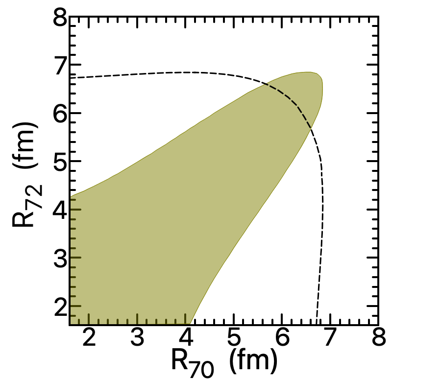
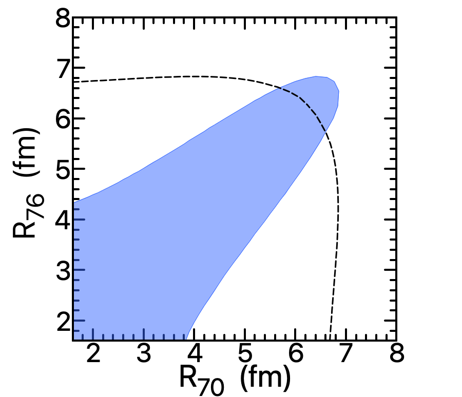
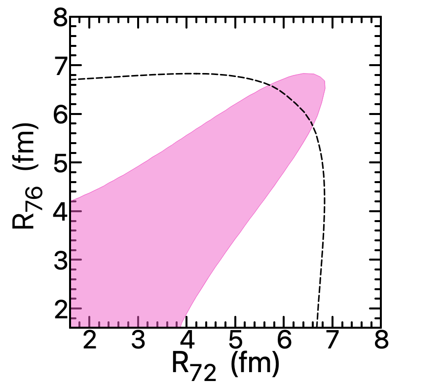
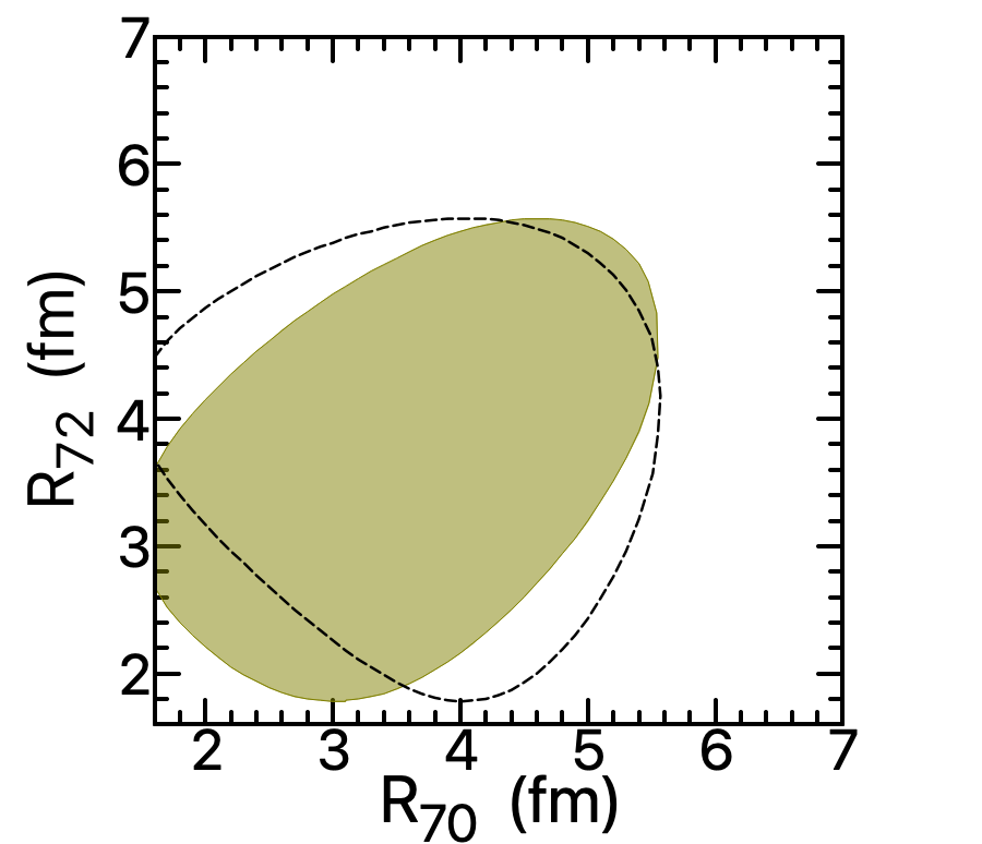
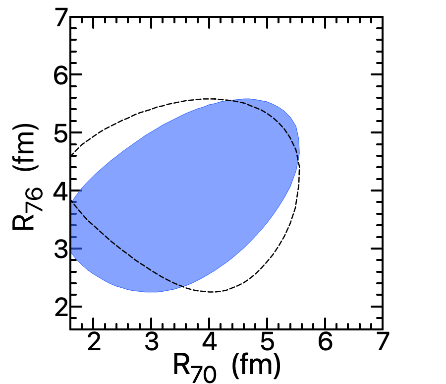
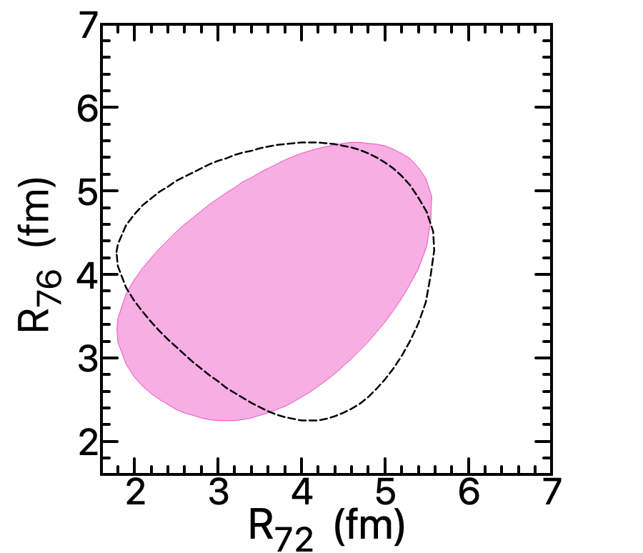
Figure 4: Neutron rms radius at a 90% C.L. for the pairs $R_{70}$ vs $R_{72}$ (left), $R_{72}$ vs $R_{76}$ (center), and $R_{70}$ vs $R_{76}$ (right), after marginalizing the information of the third isotope. In all cases the filled region represents the results when considering the correlation between detectors. The dashed line indicates the uncorrelated case. We consider background effects by adding a 10% contribution of the SM prediction to the statistical uncertainty. Top panels refer to systematic uncertainties contributions of $\sigma_{k}^{A}=$ 25% and $\sigma_{k}^{B}=$ 10% , while lower panels correspond to 5% each.

As we have pointed out, neutrinos coming from $\pi$-DAR sources are on an energy regime where the nuclear form factors play an important role in the theoretical prediction of the total number of events for a given experiment. This dependence can be used in order to constrain parameters relevant to nuclear physics as the neutron rms radius ($R_{n}$), defined as the average radius within which neutrons are distributed in the nucleus. An accurate determination of this parameter is of general interest not only for nuclear physics, but also in the characterization of Dark Matter detectors and in the experimental measurement of the neutrino floor. Currently, the neutron RMS radius has only been experimentally measured for a few elements, and the process of CEvNS can be used as a tool to determine the RMS radius of the target material. Explicitly, in the Helm parametrization of the form factor we have:

$$F_{N}^{Helm}(q^{2})=3\frac{j_{1}(qR_{0})}{qR_{0}}e^{\frac{-q^{2}s^{2}}{2}}$$ (8)

where $j_{1}(x)$ is the spherical Bessel function of order one, and $R_{0}$ satisfies:

$$R_{n}^{2}=\frac{3}{5}R_{0}^{2}+3s^{2}$$ (9)

with $s$ the neutron skin. Our proposed experimental array can be used to constrain $R_{n}$ for the involved isotope targets. To this end, we use the same set of germanium detectors under the same conditions of the analysis presented in section II for the SNS case. We perform the $\chi^{2}$ analysis, this time by considering the three neutron rms radii as our variable of interest. Fig. (4) shows the results at a 90% C.L. of the allowed regions for different radii by pairs when marginalizing the information about the other radius. Top panels refer to large contributions from systematic errors and lower panels to small contributions as in the previous section. Left panel shows the allowed values of $R_{70}$ and $R_{72}$ after marginalizing the information of $R_{76}$. The green region shows the results when we consider the correlations between systematic uncertainties, while the dashed line in the same figure represents the situation where no correlations are considered. The central panel of the same figure shows the allowed region for the pair $R_{70},R_{76}$, and the right panel shows the combination $R_{72},R_{76}$. Here we have considered the background effects as the 10% of the SM prediction in the number of events. Regardless of the configuration of systematic uncertainties, the effects of the correlations are present to a certain degree. Notice that, physically, $R_{n}>1.56$ fm according to Eq. (9). Different parameterizations exist for the distribution of both protons and neutrons within the nucleus. Another common one in the literature is the Symmetrized Fermi (SF) distribution. We have explicitly checked that similar results can be found with this case.

IV Constraining the Standard Model and non-standard interactions parameters

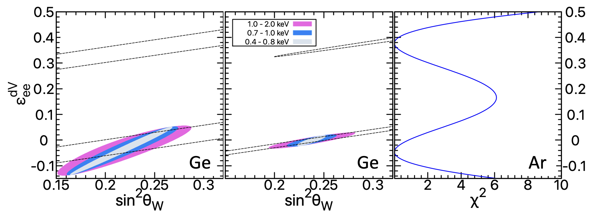
Figure 5: Allowed values at a 90% C.L. for $sin^{2}\theta_{W}$ vs $\varepsilon_{ee}^{dV}$ (left), and $\varepsilon_{ee}^{dV}$ vs $\varepsilon_{\tau e}^{dV}$ (right). In both cases the region between dashed lines represents the case where no correlations are considered. The filled curves indicate the correlated case for the three different nuclear recoil energy regions under study for reactor neutrinos. We consider the two main systematic error contributions as $\sigma_{k}^{A}=$ 25% and $\sigma_{k}^{B}=$ 10% (left) and 5% each (central). Background effects are considered by adding a 10% contribution of the SM prediction to the statistical uncertainty.

Besides constraining parameters that are relevant for nuclear physics, we can perform tests to the SM at low energies, as well as we can also get information about new physics scenarios. In the case of the SM, the weak mixing angle appears in the cross section of CEvNS through the relation:

$$g_{V}^{p}=\frac{1}{2}-2\sin^{2}\theta_{W}$$ (10)

On the other hand, we consider the formalism of Non-Standard Interactions (NSI) as the parametrization of new physics. Including these effects, the CEvNS cross section for an incoming electron (anti)neutrino now reads Barranco:2005yy :

$$\frac{\mathrm{d}\sigma}{\mathrm{d}T}\left(E_{\nu},T\right)\simeq \frac{G_{F}^{2}M}{\pi}\left(1-\frac{MT}{2E_{\nu}^{2}}\right)\left\{\left[Z\left(g_{V}^{p}+2\varepsilon_{ee}^{uV}+\varepsilon_{ee}^{dV}\right)F_{Z}^{V}(q^{2})+N\left(g_{V}^{n}+\varepsilon_{ee}^{uV}+2\varepsilon_{ee}^{dV}\right)F_{N}^{V}(q^{2})\right]^{2}\right.$$ (11)

$$\left.+\sum_{\alpha=\mu,\tau}\left[Z\left(2\varepsilon_{\alpha e}^{uV}+\varepsilon_{\alpha e}^{dV}\right)F_{Z}^{V}(q^{2})+N\left(\varepsilon_{\alpha e}^{uV}+2\varepsilon_{\alpha e}^{dV}\right)F_{N}^{V}(q^{2})\right]^{2}\right\}$$

Where $\varepsilon_{\alpha\beta}^{fV}$ are the constants that parametrize new physics. This expression contains non-universal ($\alpha=\beta$), as well as flavor changing ($\alpha\neq\beta$) parameters. In this way, we parametrize physics beyond the SM. The specific meaning of each of the couplings depends on the model under study. These include SM extensions like those considering two Higgs triplets, light mediators, non-unitarity of the mixing matrix, etc. The presence of one or more of these parameters within the cross section, can induce a degeneracy in the allowed values of the weak mixing angle, as well as in the values of NSI’s when considering two of them to be non-zero at a time. This degeneracy can be broken when using our proposed array of detectors. Here we exemplify with two different cases. To this end, we consider reactor neutrinos, since they are on an energy regime, where the form factor does not play a significant role, which allows us to study NSI parameters in a cleaner manner. Again, we perform a $\chi^{2}$ analysis assuming the two different configurations of systematic error contributions.

Fig. (5) shows the analysis when we vary the weak mixing angle and one non-universal NSI parameter ($\varepsilon_{ee}^{dV}$). The regions enclosed by dashed lines are the allowed regions at a 90% C.L. when no correlations between detectors are present. Notice that here we have two different regions, allowing values for $\sin^{2}\theta_{W}$ even smaller than 0.1 and larger than 0.4, while the NSI can take relatively large values around 0.4. In the same figure, we show the allowed regions when we consider correlations between detectors, where we have separated our results according to the three regions of the differential recoil energy defined in section II. The magenta region shows the results for the high energy tail of the spectrum $1<T<2$ keV, the blue region for $0.7<T<1$ keV, and the gray region for the low energy threshold $0.4<T<0.8$ keV. We notice that the degeneracy of the allowed values for these parameters is broken for both of the systematic error contribution scenarios. For comparison, we show the $\chi^{2}$ analysis for the current Ar data when fixing the weak mixing angle to the low-energy central value $\sin^{2}\theta_{W}=0.23865$ Miranda:2020tif . We notice that the degeneracy in the NSI parameter is also present in the Ar result. We conclude that our proposed method can be used to break this degeneracy by using a single measurement by taking advantage of the correlation between different isotopes.

A similar analysis is show in Fig. (6), this time considering the weak mixing angle fixed and varying two different NSI parameters at a time, one non-universal, and one flavor changing. The region between dashed lines shows the case when no correlations are considered, while the colored regions show the results when correlations are present under the same color code as defined in the previous case. We notice that, again, the degeneracy is broken between parameters. For comparison, we also show the current analysis for Ar data when assuming only one of each of the parameters to be non-zero at a time Miranda:2020tif . We notice that, again, the current degeneracy on the non-universal parameter can be broken by using an array of different isotopes.

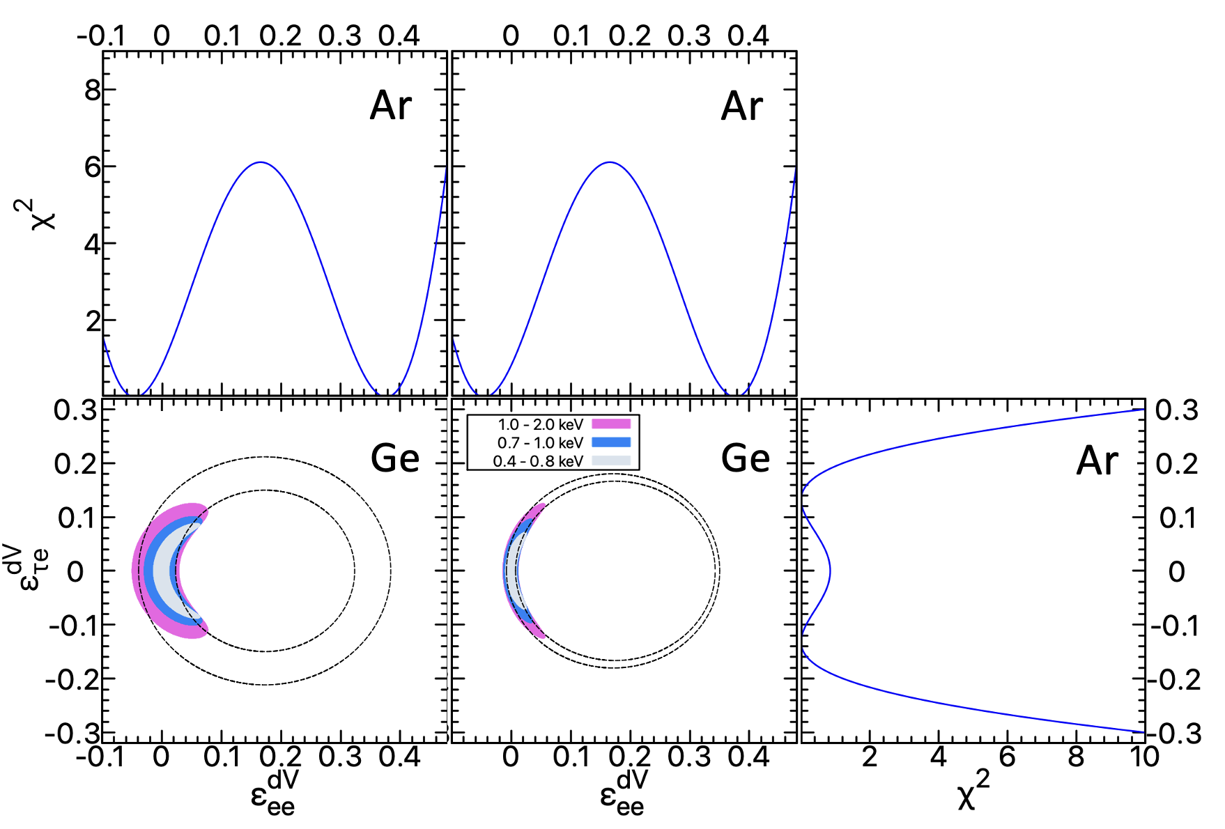
Figure 6: Allowed values at a 90% C.L. for $sin^{2}\theta_{W}$ vs $\varepsilon_{ee}^{dV}$ (left), and $\varepsilon_{ee}^{dV}$ vs $\varepsilon_{\tau e}^{dV}$ (right). In both cases the region between dashed lines represents the case where no correlations are considered. The filled curves indicate the correlated case for the three different nuclear recoil energy regions under study for reactor neutrinos. We consider the two main systematic error contributions as $\sigma_{k}^{A}=$ 25% and $\sigma_{k}^{B}=$ 10% (left) and 5% each (central). Background effects are considered by adding a 10% contribution of the SM prediction to the statistical uncertainty.

V conclusions

In summary we present a novel approach for precision measurements of CEvNS. There are no major obstacles for constructing and operating multi-isotope detector arrays based on current technologies. Detailed sensitivity studies will require of the knowledge of the detector response and background models associated with the specific experimental conditions. Second order effects in the detectors attributed to differences in the isotopic composition of its constituents will have to be taken into consideration such as departures from 100% enrichment, differences in fiducial masses, differences of quenching factors and cosmogenic and neutron-induced backgrounds Mayer:1970 ; Barabanov:2005cw .

We have shown that measuring CEvNS from the same neutrino source at the same time with several isotopically enriched detectors will improve the accuracy of the measurement. We have illustrated this idea with a well motivated array based on three different germanium isotopes and applied to the concrete example of confirming the $N^{2}$ rule. We have also illustrated how, in the case of a $\pi$-DAR neutrino flux, the measurement of the mean neutron radius can be improved. For the reactor antineutrino case, we have shown how the proposed array can provide a robust test for new physics The proposal discussed here will help to achieve the necessary accuracy to untangle different contributions from nuclear and particle physics allowing for a reliable constraint on physics beyond the SM that would be free from neutron charge distribution uncertainties AristizabalSierra:2019zmy and can resolve the characteristic degeneracies appearing in these scenarios. The same technique can be applied to other technologies that allow lower energy thresholds as in the case of bolometers. After the first detection of CEvNS at the SNS, the next generation of experiments will aim for precision measurements. Despite several years and a worldwide effort, detection of CEvNS at a reactor has not been observed. Neutrino fluxes and quenching factors remain as considerable sources of uncertainty. We have shown that with the current level of uncertainties, this proposed array would allow a clear signature of (anti)neutrino detection, keeping the different systematics under control. Our combinations of systematic error contributions show how future improvements on the systematics will improve the accuracy of the measurements for different observables.

This work was performed under the auspices of the U.S. Department of Energy by Oak Ridge National Laboratory under Contract No. DE-AC05- 00OR22725. This work has been supported by CONACyT under grant A1-S-23238. The authors appreciate discussions with J. Collar, Chicago, and B. Littlejohn, Illinois Tech.

References

- (1) D. Z. Freedman, Phys. Rev. D 9, 1389 (1974). doi:10.1103/PhysRevD.9.1389
- (2) D. Akimov et al. [COHERENT Collaboration], Science 357, no. 6356, 1123 (2017) doi:10.1126/science.aao0990 [arXiv:1708.01294 [nucl-ex]].
- (3) D. Akimov et al. [COHERENT Collaboration], doi:10.5281/zenodo.1228631 arXiv:1804.09459 [nucl-ex].
- (4) D. Akimov et al. [COHERENT Collaboration], Phys. Rev. D 100, no. 11, 115020 (2019) doi:10.1103/PhysRevD.100.115020 [arXiv:1909.05913 [hep-ex]].
- (5) D. Akimov et al. [COHERENT], [arXiv:2003.10630 [nucl-ex]].
- (6) M. Cadeddu, C. Giunti, Y. F. Li and Y. Y. Zhang, Phys. Rev. Lett. 120 (2018) no.7, 072501 doi:10.1103/PhysRevLett.120.072501 [arXiv:1710.02730 [hep-ph]].
- (7) D. K. Papoulias, T. S. Kosmas, R. Sahu, V. K. B. Kota and M. Hota, Phys. Lett. B 800 (2020), 135133 doi:10.1016/j.physletb.2019.135133 [arXiv:1903.03722 [hep-ph]].
- (8) D. Aristizabal Sierra, J. Liao and D. Marfatia, JHEP 06 (2019), 141 doi:10.1007/JHEP06(2019)141 [arXiv:1902.07398 [hep-ph]].
- (9) P. Coloma, I. Esteban, M. C. Gonzalez-Garcia and J. Menendez, JHEP 08 (2020) no.08, 030 doi:10.1007/JHEP08(2020)030 [arXiv:2006.08624 [hep-ph]].
- (10) M. Hoferichter, J. Menéndez and A. Schwenk, Phys. Rev. D 102, no.7, 074018 (2020) doi:10.1103/PhysRevD.102.074018 [arXiv:2007.08529 [hep-ph]].
- (11) O. Tomalak, P. Machado, V. Pandey and R. Plestid, [arXiv:2011.05960 [hep-ph]].
- (12) J. Barranco, O. G. Miranda and T. I. Rashba, JHEP 12 (2005), 021 doi:10.1088/1126-6708/2005/12/021 [arXiv:hep-ph/0508299 [hep-ph]].
- (13) K. Scholberg, a stopped-pion neutrino source,” Phys. Rev. D 73 (2006), 033005 doi:10.1103/PhysRevD.73.033005 [arXiv:hep-ex/0511042 [hep-ex]].
- (14) J. Billard, J. Johnston and B. J. Kavanagh, JCAP 11 (2018), 016 doi:10.1088/1475-7516/2018/11/016 [arXiv:1805.01798 [hep-ph]].
- (15) Y. Farzan, M. Lindner, W. Rodejohann and X. J. Xu, JHEP 05 (2018), 066 doi:10.1007/JHEP05(2018)066 [arXiv:1802.05171 [hep-ph]].
- (16) H. T. Wong, Nucl. Phys. B Proc. Suppl. 138 (2005), 333-336 doi:10.1016/j.nuclphysbps.2004.11.076 [arXiv:hep-ex/0311001 [hep-ex]].
- (17) O. G. Miranda, D. K. Papoulias, M. Tórtola and J. W. F. Valle, JHEP 07 (2019), 103 doi:10.1007/JHEP07(2019)103 [arXiv:1905.03750 [hep-ph]].
- (18) B. Dutta, Y. Gao, R. Mahapatra, N. Mirabolfathi, L. E. Strigari and J. W. Walker, Phys. Rev. D 94 (2016) no.9, 093002 doi:10.1103/PhysRevD.94.093002 [arXiv:1511.02834 [hep-ph]].
- (19) B. C. Cañas, E. A. Garcés, O. G. Miranda and A. Parada, Phys. Lett. B 776 (2018), 451-456 doi:10.1016/j.physletb.2017.11.074 [arXiv:1708.09518 [hep-ph]].
- (20) O. G. Miranda, D. K. Papoulias, O. Sanders, M. Tórtola and J. W. F. Valle, [arXiv:2008.02759 [hep-ph]].
- (21) M. Bowen and P. Huber, [arXiv:2005.10907 [physics.ins-det]].
- (22) J. I. Collar, A. R. L. Kavner and C. M. Lewis, Phys. Rev. D 100, no.3, 033003 (2019) doi:10.1103/PhysRevD.100.033003 [arXiv:1907.04828 [nucl-ex]].
- (23) J. I. Collar, A. R. L. Kavner and C. M. Lewis, Phys. Rev. D 103 (2021) no.12, 122003 doi:10.1103/PhysRevD.103.122003 [arXiv:2102.10089 [nucl-ex]].
- (24) R. Tayloe, Magnificent CEvNS, October 2021. https://indi.to/v2zGS
- (25) D. Akimov, P. An, C. Awe, P. S. Barbeau, B. Becker, V. Belov, I. Bernardi, M. A. Blackston, C. Bock and A. Bolozdynya, et al. [arXiv:2110.07730 [hep-ex]].
- (26) A. Aguilar-Arevalo et al. [CONNIE Collaboration], JINST 11, no. 07, P07024 (2016) doi:10.1088/1748-0221/11/07/P07024 [arXiv:1604.01343 [physics.ins-det]].
- (27) A. Aguilar-Arevalo et al. [CONNIE Collaboration], Phys. Rev. D 100, no. 9, 092005 (2019) doi:10.1103/PhysRevD.100.092005 [arXiv:1906.02200 [physics.ins-det]].
- (28) D. Akimov et al. [COHERENT Collaboration], arXiv:1803.09183 [physics.ins-det].
- (29) M. Lindner, W. Rodejohann and X. J. Xu, JHEP 1703, 097 (2017) doi:10.1007/JHEP03(2017)097 [arXiv:1612.04150 [hep-ph]].
- (30) V. Belov et al., J. Instrum. 10, P12011 (2015).
- (31) H. T. Wong, H. B. Li, J. Li, Q. Yue and Z. Y. Zhou, J. Phys. Conf. Ser. 39 (2006), 266-268 doi:10.1088/1742-6596/39/1/064 [arXiv:hep-ex/0511001 [hep-ex]].
- (32) G. Agnolet et al. [MINER], Nucl. Instrum. Meth. A 853 (2017), 53-60 doi:10.1016/j.nima.2017.02.024 [arXiv:1609.02066 [physics.ins-det]].
- (33) G. Angloher et al. [NUCLEUS], Eur. Phys. J. C 79 (2019) no.12, 1018 doi:10.1140/epjc/s10052-019-7454-4 [arXiv:1905.10258 [physics.ins-det]].
- (34) J. Billard, et al. J. Phys. G 44 (2017) no.10, 105101 doi:10.1088/1361-6471/aa83d0 [arXiv:1612.09035 [physics.ins-det]].
- (35) M. Gunther, et al.. [Heidelberg-Moscow Collaboration], Phys. Rev. D 55, 54-67 (1997) doi:10.1103/PhysRevD.55.54
- (36) K. P. Gradwohl, O. Moras, J. Janicsko-Csathy, S. Schonert and R. R. Sumathi, [arXiv:2009.07585 [physics.ins-det]].
- (37) D. Budjas, et al.. JINST 8, P04018 (2013) doi:10.1088/1748-0221/8/04/P04018 [arXiv:1303.6768 [physics.ins-det]].
- (38) M. Agostini et al. Nucl. Phys. B Proc. Suppl. 229-232, 489-489 (2012) doi:10.1016/j.nuclphysbps.2012.09.126
- (39) D. Akimov et al. [COHERENT], [arXiv:1509.08702 [physics.ins-det]].
- (40) P. Huber and T. Schwetz, Phys. Rev. D 70 (2004), 053011 doi:10.1103/PhysRevD.70.053011 [arXiv:hep-ph/0407026 [hep-ph]].
- (41) G. Mention, M. Fechner, T. Lasserre, T. A. Mueller, D. Lhuillier, M. Cribier and A. Letourneau, Phys. Rev. D 83 (2011), 073006 doi:10.1103/PhysRevD.83.073006 [arXiv:1101.2755 [hep-ex]].
- (42) V. I. Kopeikin, L. A. Mikaelyan and V. V. Sinev, Phys. Atom. Nucl. 60 (1997), 172-176
- (43) O. G. Miranda, D. K. Papoulias, G. Sanchez Garcia, O. Sanders, M. Tórtola and J. W. F. Valle, JHEP 05 (2020), 130 [erratum: JHEP 01 (2021), 067] doi:10.1007/JHEP05(2020)130 [arXiv:2003.12050 [hep-ph]].
- (44) J. W. Mayer, L. Eriksson, and J.A. Davis, Ion Implantation in Semiconductors (Academic, New York, 1970). doi.org/10.1016/B978-0-12-480850-8.X5001-6
- (45) I. Barabanov, S. Belogurov, L. B. Bezrukov, A. Denisov, V. Kornoukhov and N. Sobolevsky, Nucl. Instrum. Meth. B 251 (2006), 115-120 doi:10.1016/j.nimb.2006.05.011 [arXiv:nucl-ex/0511049 [nucl-ex]].