Unmixing methods based on nonnegativity and weakly mixed pixels for astronomical hyperspectral datasets

An increasing number of astronomical instruments (on Earth and space-based) provide hyperspectral images, that is three-dimensional data cubes with two spatial dimensions and one spectral dimension. The intrinsic limitation in spatial resolution of these instruments implies that the spectra associated with pixels of such images are most often mixtures of the spectra of the “pure” components that exist in the considered region. In order to estimate the spectra and spatial abundances of these pure components, we here propose an original blind signal separation (BSS), that is to say an unsupervised unmixing method. Our approach is based on extensions and combinations of linear BSS methods that belong to two major classes of methods, namely nonnegative matrix factorization (NMF) and Sparse Component Analysis (SCA). The former performs the decomposition of hyperspectral images, as a set of pure spectra and abundance maps, by using nonnegativity constraints, but the estimated solution is not unique: It highly depends on the initialization of the algorithm. The considered SCA methods are based on the assumption of the existence of points or tiny spatial zones where only one source is active (i.e., one pure component is present). These points or zones are then used to estimate the mixture and perform the decomposition. In real conditions, the assumption of perfect single-source points or zones is not always realistic. In such conditions, SCA yields approximate versions of the unknown sources and mixing coefficients. We propose to use part of these preliminary estimates from the SCA to initialize several runs of the NMF in order to refine these estimates and further constrain the convergence of the NMF algorithm. The proposed methods also estimate the number of pure components involved in the data and they provide error bars associated with the obtained solution. Detailed tests with synthetic data show that the decomposition achieved with such hybrid methods is nearly unique and provides good performance, illustrating the potential of applications to real data.

1 Introduction

Telescopes keep growing in diameter, and detectors are more and more sensitive and made up of an increasing number of pixels. Hence, the number of photons that can be captured by astronomical instruments, in a given amount of time and at a given wavelength, has increased significantly, thus allowing astronomy to go hyperspectral. More and more, astronomers do not deal with 2D images or 1D spectra, but with a combination of these media resulting in three-dimensional (3D) data cubes (two spatial dimensions, one spectral dimension). We hereafter provide an overview of the instruments that provide hyperspectral data in astronomy, mentioning specific examples without any objective to be exhaustive. Several integral field unit spectrographs (e.g., MUSE on the Very Large Telescope) provide spectral cubes at visible wavelengths, yielding access to the optical tracers of ionized gas (see for instance Weilbacher et al. 2015). Infrared missions such as the Infrared Space Observatory (ISO) and Spitzer performed spectral mapping in the mid-infrared, a domain that is particularly suited to observe the emission of UV heated polycyclic aromatic hydrocarbon (e.g., Cesarsky et al. 1996; Werner et al. 2004). In the millimeter wavelengths, large spectral maps in rotational lines of abundant molecules (typically CO) have been used for several decades to trace the dynamics of molecular clouds (e.g., Bally et al. (1987); Miesch & Bally (1994); Falgarone et al. (2009)). The PACS, SPIRE, and HIFI instruments, on board Herschel all have a mode that allows for spectral mapping (e.g. Van Kempen et al. 2010; Habart et al. 2010; Joblin et al. 2010) in atomic and molecular lines. Owing to its high spectral resolution, HIFI allows one to resolve the profiles of these lines, enabling one to study the kinematics of, for example, the immediate surroundings of protostars (Kristensen et al. (2011)) or of star-forming regions (Pilleri et al. (2012)) using radiative transfer models. Similarly, the GREAT instrument on board the Stratospheric Observatory For Infrared Astronomy (SOFIA) now provides large-scale spectral maps in the C⁺ line at 1.9 THz (Pabst et al. (2017)). The Atacama Large Millimeter Array (ALMA) also provides final products that are spectral cubes (see e.g., Goicoechea et al. (2016)). A majority of astronomical spectrographs to be employed at large observatories in the future will provide spectral maps. This is the case for the MIRI and NISPEC instruments on the James Webb Space Telescope (JWST) and the METIS instrument on the Extremely Large Telescope (ELT).

Although such 3D datasets have become common, few methods have been developed by astronomers to analyze the outstanding amount of information they contain. Classical analysis methods tend to decompose the spectra by fitting them with simple functions (typically mixtures of Gaussians) but this has several disadvantages: 1) the a priori assumption made by the use of a given function is usually not founded physically, 2) if the number of parameters is high, the result of the fit may be degenerate, 3) for large datasets and fitting with nonlinear functions, the fitting may be very time consuming, 4) initial guesses must be provided, and, 5) the spectral fitting is usually performed on a (spatial) pixel by pixel basis, so that the extracted components are spatially independent, whereas physical components are often present at large scales on the image. An alternative is to analyze the data by means of principal component analysis (e.g., Neufeld et al. 2007; Gratier et al. 2017), which provides a representation of the data in an orthogonal basis of a subspace, thus allowing interpretation. However, this may be limited by the fact that the principal components are orthogonal, and hence they are not easily interpretable in physical terms. An alternative analysis was proposed by Juvela et al. (1996), which is based on a Blind Signal Separation (BSS) approach. It consists in decomposing spectral cubes (in their case, CO spectral maps) into the product of a small number of spectral components, or “end members”, and spatial “abundance” maps.

This requires no a priori on spectral properties of the components, and hence this can provide deeper insights into the physical structure represented in the data, as demonstrated in this pioneering paper. This method uses the positivity constraint for the maps and spectra (all their points must be positive) combined with the minimization of a statistical criterion to derive the maps and spectral components. This method is referred to as positive matrix factorization (PMF, Paatero & Tapper (1994)). Although it contained the original idea of using positivity as a constraint to estimate a matrix product, this work used a classical optimization algorithm. Several years later, Lee & Seung (1999) introduced a novel algorithm to perform PMF using simple multiplicative iterative rules, making the PMF algorithm extremely fast. This algorithm is usually referred to as Lee and Seung’s Non Negative Matrix Factorization (NMF hereafter) and has been widely used in a vast number of applications outside astronomy. This algorithm has proved to be efficient including in astrophysical applications (Berné et al., 2007). However, NMF has several disadvantages: 1) the number of spectra to be extracted must be given by the user, 2) the error bars related to the procedure are not derived automatically, 3) convergence to a unique point is not guaranteed and may depend on initialization (see Donoho & Stodden 2003 on these latter aspects). When applying NMF to astronomical hyperspectral data, the above drawbacks become critical and can jeopardize the integrity of the results.

In this paper, we evaluate possibilities to improve application of BSS to hyperspectral positive data by hybridizing NMF with sparsity-based algorithms. Here, we focus on synthetic data, so as to perform a detailed comparison of the performances of the proposed approaches. A first application on real data of one of the methods presented here is provided in Foschino et al. (2019). The proposed methods should be applicable to any hyperspectral dataset fulfilling the properties that we will describe hereafter. The paper is organized as follows. In the next section we present the adopted mathematical model for hyperspectral astronomical data, using tow possible conventions, spatial or spectral. We describe the mixing model and associated “blind signal separation” (BSS) problem. In Section 3, we describe the preliminary steps (preprocessing steps) that are required before applying the proposed algorithms. In Section 4 we describe in details the three methods that are used in this paper, that is, NMF (with an extension using a Monte-Carlo approach referred to as MC-NMF) and two methods based on sparsity (Space-CORR and Maximum Angle Source Separation, MASS). We then detail how MC-NMF can be hybridized with the latter two methods.

In Section 5, a comparative performance analysis of studied methods is performed. We conclude in Section 6.

2 Data model and blind source separation problem

The observed data consist of a spectral cube $\underline{C}(p_{x},p_{y},f)$ of dimension $P_{x}\times P_{y}\times N$ where ($p_{x},p_{y}$) define the spatial coordinates and $f$ is the spectral index. To help one interpret the results, the spectral index is hereafter expressed as a Doppler-shift velocity in km/s, using $v=c\times(f-f_{0})/f_{0}$, with $f$ the observed frequency, $f_{0}$ the emitted frequency and $c$ the light speed. We assume that all observed values in $\underline{C}$ are nonnegative. We call each vector $\underline{C}(p_{x},p_{y},.)$ recorded at a position ($p_{x},p_{y}$) “spectrum” and we call each matrix $\underline{C}(.,.,v)$ recorded at a given velocity “spectral band.” Each observed spectrum corresponding to a given pixel results from a mixture of different kinematic components that are present on the line of sight of the instrument. Mathematically, the observed spectrum obtained for one pixel is then a combination (which will be assumed to be linear and instantaneous) of elementary spectra.

In order to recover these elementary spectra, one can use methods known as Blind Source Separation (BSS). BSS consists in estimating a set of unknown source signals from a set of observed signals that are mixtures of these source signals. The linear mixing coefficients are unknown and are also to be estimated. The observed spectral cube is then decomposed as a set of elementary spectra and a set of abundance maps (the contributions of elementary spectra in each pixel).

Considering BSS terminology and a linear mixing model, the matrix containing all observations is expressed as the product of a mixing matrix and a source matrix. Therefore, it is necessary here to restructure the hyperspectral cube $\underline{C}$ into a matrix and to identify what we call “observations”, “samples”, “mixing coefficients”, and “sources”. A spectral cube can be modeled in two different ways: a spectral model where we consider the cube as a set of spectra and a spatial model where we consider the cube as a set of images (spectral bands), as detailed hereafter.

2.1 Spectral model

Table 1: List of major variables

Variable	Description
$spec(l,v)$	Value of elementary spectrum $l$ at velocity index $v$
$Spec$	Matrix of values $spec(l,v)$ of elementary spectra
$map(m,l)$	Scale factor of elementary spectrum $p$ in pixel $m$
$Map$	Matrix of scale factors $map(m,l)$
$obs(m,v)$	Observed value of pixel $m$ at velocity $v$
$Obs$	Matrix of observed values $obs(m,v)$

For the spectral data model, we define the observations as being the spectra $\underline{C}(p_{x},p_{y},.)$. The data cube $\underline{C}$ is reshaped into a new matrix of observations $Obs$ (variables defined in this section are summarized in Table 1), where the rows contain the $P_{x}\times P_{y}=M$ observed spectra of $\underline{C}$ arranged in any order and indexed by $m$. Each column of $Obs$ corresponds to a given spectral sample with an integer-valued index also denoted as $v\in\{1,\ldots,N\}$ for all observations. Each observed spectrum $obs(m,.)$ is a linear combination of $L$ ($L\ll M$) unknown elementary spectra and yields a different mixture of the same elementary spectra:

$$obs(m,v)=\sum_{\ell=1}^{L}map(m,\ell)\leavevmode\nobreak\ spec(\ell,v)$$ (1)

$$m\in\{1,\ldots,M\},\leavevmode\nobreak\ v\in\{1,\ldots,N\},\ell\in\{1,\ldots,L\},$$

where $obs(m,v)$ is the $v^{th}$ sample of the $m^{th}$ observation, $spec(\ell,v)$ is the $v^{th}$ sample of the $\ell^{th}$ elementary spectrum and $map(m,\ell)$ defines the contribution scale of elementary spectrum $\ell$ in observation $m$. Using the BSS terminology, $map$ stands for the mixing coefficients and $spec$ stands for the sources. This model can be rewritten in matrix form:

$$Obs=Map\times Spec,$$ (2)

where $Map$ is an $M\times L$ mixing matrix and $Spec$ is an $L\times N$ source matrix.

2.2 Spatial model

For the spatial data model, we define the observations as being the spectral bands $\underline{C}(.,.,v)$. The construction of the spatial model is performed by transposing the spectral model (2). In this configuration, the rows of the observation matrix $Obs^{T}$ (the transpose of the original matrix of observations $Obs$) contain the $N$ spectral bands with a one-dimensional structure. Each column of $Obs^{T}$ corresponds to a given spatial sample index $m\in\{1,\ldots,M\}$ for all observations (i.e., each column corresponds to a pixel). Each spectral band $Obs^{T}(v,.)$ is a linear combination of $L$ ($L\ll N$) unknown abundance maps and yields a different mixture of the same abundance maps:

$$Obs^{T}=Spec^{T}\times Map^{T},$$ (3)

where $Obs^{T}$ is the transpose of the original observation matrix, $Spec^{T}$ is the $N\times L$ mixing matrix and $Map^{T}$ is the $L\times M$ source matrix. In this alternative data model, the elementary spectra in $Spec^{T}$ stand for the mixing coefficients and the abundance maps in $Map^{T}$ stand for the sources.

2.3 Problem statement

In this section, we denote the mixing matrix as $A$ and the source matrix as $S$, whatever the nature of the adopted model (spatial or spectral) to simplify notations, the following remarks being valid in both cases.

The goal of BSS methods is to find estimates of a mixing matrix $A$ and a source matrix $S$, respectively denoted as $\hat{A}$ and $\hat{S}$, and such that:

$$X\approx\hat{A}\hat{S}.$$ (4)

However this problem is ill-posed. Indeed, if $\{\hat{A},\hat{S}\}$ is a solution, then $\{\hat{A}P^{-1},P\hat{S}\}$ is also a solution for any invertible matrix $P$. To achieve the decomposition, we must add two extra constraints. The first one is a constraint on the properties of the unknown matrices $\hat{A}$ and/or $\hat{S}$. The type of constraint (independence of sources, nonnegative matrices, sparsity) leads directly to the class of methods that will be used for the decomposition. The case of linear instantaneous mixtures was first studied in the 1980s, then three classes of methods became important:

• Independent component analysis (ICA) (Cardoso (1998); Hyvärinen et al. (2001)): It is based on a probabilistic formalism and requires the source signals to be mutually statistically independent. Until the early 2000s, ICA was the only class of methods available to achieve BSS.

• Nonnegative matrix factorization (NMF) (Lee & Seung (1999)): It requires the source signals and mixing coefficients values to be nonnegative.

• Sparse component analysis (SCA) (Gribonval & Lesage (2006)): It requires the source signals to be sparse in the considered representation domain (time, time-frequency, time-scale, wavelet…).

The second constraint is to determine the dimensions of $\hat{A}$ and $\hat{S}$. Two of these dimensions are obtained directly from observations $X$ ($M$ and $N$). The third dimension, common to both $\hat{A}$ and $\hat{S}$ matrices, is the number of sources $L$, which must be estimated.

Here, we consider astrophysical hyperspectral data that have the properties listed below. These are relatively general properties that are applicable to a number of cases with Herschel-HIFI, ALMA, Spitzer, JWST, etc:

• They do not satisfy the condition of independence of the sources. In our simulated data, elementary spectra have, by construction, similar variations (Gaussian spectra with different means, see Section 5.1). Likewise, abundance maps associated with each elementary spectrum have similar shapes. Such data involve nonzero correlation coefficients between elementary spectra and between abundance maps. Hence ICA methods will not be discussed in this paper.

• These data are nonnegative if we disregard noise. Each pixel provides an emission spectrum, hence composed of positive or zero values. Such data thus correspond to the conditions of use of NMF that we detail in Section 4.1.

• If we consider the data in a spatial framework (spatial model), the cube provides a set of images. We can then formulate the hypothesis that there are regions in these images where only one source is present. This is detailed in Section 4.2. This hypothesis then refers to a “sparsity” assumption in the data and SCA methods are then applicable to hyperspectral cubes. On the contrary, sparsity properties do not exist in the spectral framework in our case, as discussed below.

• If the data have some sparsity properties, adding the nonnegativity assumption enables the use of geometric methods. The geometric methods are a subclass of BSS methods based on the identification of the convex hull containing the mixed data. However, the majority of geometric methods, which are used in hyperspectral unmixing in Earth observation, are not applicable to Astrophysics because they set an additional constraint on the data model: they require all abundance coefficients to sum to one in each pixel, which changes the geometrical representation of the mixed data. On the contrary, in Section 4.3, we introduce a geometric method called MASS, for Maximum Angle Source Separation (Boulais et al. (2015)), which may be used in an astrophysical context (i.e., for data respecting the models presented above).

The sparsity constraint required for SCA and geometric methods is carried by the source matrix $S$. These methods may therefore potentially be applied in two ways to the above-defined data: either we suppose that there exist spectral indices for which a unique spectral source is nonzero, or we suppose that there exist some regions in the image for which a unique spatial source is zero. In our context of studying the properties of photodissociation regions, only the second case is realistic. Thus only the mixing model (3) is relevant. Therefore, throughout the rest of this paper, we will only use that spatial data model (3), so that we here define the associated final notations and vocabulary: let $X=Obs^{T}$ be the $(N\times M)$ observation matrix, $A=Spec^{T}$ the $(N\times L)$ mixing matrix containing the elementary spectra and $S=Map^{T}$ the $(L\times M)$ source matrix containing the spatial abundance maps, each associated with an elementary spectrum.

Moreover, we note that in the case of the NMF, the spectral and spatial models are equivalent but the community generally prefers the more intuitive spectral model.

Before thoroughly describing the algorithms used for the aforementioned BSS methods, we present preprocessing stages required for the decomposition of data cubes.

3 Data preprocessing

3.1 Estimation of number of sources

An inherent problem in BSS is to estimate the number $L$ of sources (the dimension shared by the $\hat{A}$ and $\hat{S}$ matrices). This parameter should be fixed before performing the decomposition in the majority of cases. Here, this estimate is based on the eigen-decomposition of the covariance matrix of the data. As in Principal Component Analysis (PCA), we look for the minimum number of components that most contribute to the total variance of the data. Thus the number of high eigenvalues is the number of sources in the data. Let $\Sigma_{X}$ be the $(N\times N)$ covariance matrix of observations $X$:

$$\Sigma_{X}=\frac{1}{M}X_{c}X_{c}^{T}=\sum_{i=1}^{N}\lambda_{i}e_{i}e_{i}^{T},$$ (5)

where $\lambda_{i}$ is the $i^{th}$ eigenvalue associated with eigenvector $e_{i}$ and $X_{c}$ is the matrix of centered data (i.e. each observation has zero mean: $x_{c}(n,.)=x(n,.)-\bar{x}(n,.)$ ).

The eigenvalues of $\Sigma_{X}$ have the following properties (their proofs are available in Deville et al. (2014)):

Property 1: For noiseless data ($X_{0}=AS$), the $\Sigma_{X}$ matrix has $L$ positive eigenvalues and $N-L$ eigenvalues equal to zero.

The number $L$ of sources is therefore simply inferred from this property. Now, we consider the data with an additive spatially white noise $E$, with standard deviation $\sigma_{E}$, i.e., $X=X_{0}+E$. The relation between the covariance matrix $\Sigma_{X_{0}}$ of noiseless data and the covariance matrix $\Sigma_{X}$ of noisy data is then:

$$\Sigma_{X}=\Sigma_{X_{0}}+\sigma_{E}^{2}I_{N},$$ (6)

where $I_{N}$ is the identity matrix.

Property 2: The eigenvalues $\lambda$ of $\Sigma_{X}$ and the eigenvalues $\lambda_{0}$ of $\Sigma_{X_{0}}$ are linked by:

$$\lambda=\lambda_{0}+\sigma_{E}^{2}.$$ (7)

These two properties then show that the ordered eigenvalues $\lambda_{(i)}$ of $\Sigma_{X}$ for a mixture of $L$ sources are such that:

$$\lambda_{(1)}\geq\ldots\geq\lambda_{(L)}>\lambda_{(L+1)}=\ldots=\lambda_{(N)}=\sigma_{E}^{2}.$$ (8)

But in practice, because of the limited number of samples and since the strong assumption of a white noise with the same standard deviation in all pixels is not fulfilled, the equality $\lambda_{(L+1)}=\ldots=\lambda_{(N)}=\sigma_{E}^{2}$ is not met. However, the differences between the eigenvalues $\lambda_{(L+1)},\ldots,{\color[rgb]{0,0,0}\lambda_{(N)}}$ are small compared to the differences between the eigenvalues $\lambda_{(1)},\ldots,\lambda_{(L)}$. The curve of the ordered eigenvalues is therefore constituted of two parts. The first part, $\Omega_{S}$, contains the first $L$ eigenvalues associated with a strong contribution in the total variance. In this part, eigenvalues are significantly different. The second part, $\Omega_{E}$, contains the other eigenvalues, associated with noise. In this part, eigenvalues are similar.

The aim is then to identify from which rank $r=L+1$ eigenvalues no longer vary significantly. To this end, we use a method based on the gradient of the curve of ordered eigenvalues (Luo & Zhang (2000)) in order to identify a break in this curve (see Fig. 5).

Moreover, a precaution must be taken concerning the difference between $\lambda_{(L)}$ and $\lambda_{(L+1)}$. In simulations, we found that in the noiseless case, it is possible that the last eigenvalues of $\Omega_{S}$ are close to zero. Thus, for very noisy mixtures, the differences between these eigenvalues become negligible relative to the noise variance $\sigma_{E}^{2}$. These eigenvalues are then associated with $\Omega_{E}$ and therefore rank $r$ where a “break” appears will be underestimated.

The procedure described by Luo & Zhang (2000) is as follows:

1. Compute the eigen-decomposition of the covariance matrix $\Sigma_{X}$ and arrange the eigenvalues in decreasing order.

2. Compute the gradient of the curve of the logarithm of the $L$ first (typically $L=20$) ordered eigenvalues:

   $$\nabla\lambda_{(i)}=\ln(\lambda_{(i)}/\lambda_{(i+1)})\qquad i\in{1,\ldots,L}.$$ (9)

3. Compute the average gradient of all these eigenvalues:

   $$\overline{\nabla\lambda}=\frac{1}{(L-1)}\ln(\lambda_{(1)}/\lambda_{(L)}).$$ (10)

4. Find all $i$ satisfying $\nabla\lambda_{(i)}<\overline{\nabla\lambda}$ to construct the set $\{\mathcal{I}\}=\{i\leavevmode\nobreak\ |\leavevmode\nobreak\ \nabla\lambda_{(i)}<\overline{\nabla\lambda}\}$.

5. Select the index $r$, such that it is the first one of the last continuous block of $i$ in the set $\{\mathcal{I}\}$.

6. The number of sources is then $L=r-1$.

3.2 Noise reduction

The observed spectra are contaminated by noise. In synthetic data, this noise is added assuming it is white and Gaussian. Noise in real data may have different properties, however the aforementioned assumptions are made here in order to evaluate the sensitivity of the method to noise in the general case. To improve the performance of the above BSS methods, we propose different preprocessing stages to reduce the influence of noise on the results.

The first preprocessing stage consists of applying a spectral thresholding, i.e., only the continuous range of $v$ containing signal is preserved. Typically many first and last channels contain only noise and are therefore unnecessary for the BSS. This is done for all BSS methods presented in the next section.

The second preprocessing stage consists of applying a spatial thresholding. Here, we must distinguish the case of each BSS method because the SCA method requires to retain the spatial structure of data. For NMF, the observed spectra (columns of $X$) whose “normalized power” is lower than a threshold $\alpha_{e}$ are discarded. Typically some spectra contain only noise and are therefore unnecessary for the spectra estimation step (Section 4.1). In our application, we set the threshold to $\alpha_{e}=\max\limits_{i}\|X{\color[rgb]{0,0,0}(.,i)}\|\times 0.2\leavevmode\nobreak\ \leavevmode\nobreak\ (\forall i\in\{1,\ldots,{\color[rgb]{0,0,0}M}\})$. For the SCA method, some definitions are necessary to describe this spatial thresholding step. This procedure is therefore presented in the section regarding the method itself (Section 4.2).

Finally, synthetic and actual data from the HIFI instrument contain some negative values due to noise. To stay in the assumption of NMF, these values are reset to $\epsilon=10^{-16}$.

4 Blind signal separation methods

4.1 nonnegative matrix factorization and our extension

NMF is a class of methods introduced by Lee & Seung (1999). The standard algorithm iteratively and simultaneously computes $\hat{A}$ and $\hat{S}$, minimizing an objective function of the initial $X$ matrix and the $\hat{A}\hat{S}$ product. In our case, we use the minimization of the Euclidean distance $\delta=\frac{1}{2}\|X-\hat{A}\hat{S}\|^{2}_{F}$, using multiplicative update rules:

$$\hat{A}\leftarrow\hat{A}\odot(X\hat{S}^{T})\oslash(\hat{A}\hat{S}\hat{S}^{T})$$ (11)

$$\hat{S}\leftarrow\hat{S}\odot(\hat{A}^{T}X)\oslash(\hat{A}^{T}\hat{A}\hat{S}),$$ (12)

where $\odot$ and $\oslash$ are respectively the element-wise product and division.

Lee and Seung show that the Euclidean distance $\delta$ is non increasing under these update rules (Lee & Seung (2001)), so that starting from random $\hat{A}$ and $\hat{S}$ matrices, the algorithm will converge toward a minimum for $\delta$. We estimate that the convergence is reached when:

$$1-\frac{\delta^{i+1}}{\delta^{i}}<\kappa,$$ (13)

where $i$ corresponds to the iteration and $\kappa$ is a threshold typically set to $10^{-4}$.

The main drawback of standard NMF is the uniqueness of the decomposition. The algorithm is sensitive to the initialization due to the existence of local minima of the objective function (Cichocki et al. (2009)). The convergence point highly depends on the distance between the initial point and a global minimum. A random initialization without additional constraint is generally not satisfactory. To improve the quality of the decomposition, several solutions are possible:

• Use a Monte-Carlo analysis to estimate the elementary spectra and then rebuild the abundance maps (Berné et al. (2012)).

• Further constrain the convergence by altering the initialization (Langville et al. (2006)).

• Use additional constraints on the sources and/or mixing coefficients, such as sparsity constraints (Cichocki et al. (2009)), or geometric constraints (Miao & Qi (2007)).

The addition of geometric constraints is usually based on the sum-to-one of the abundance coefficients for each pixel ($\sum\limits_{\ell=1}^{L}s_{m}(\ell)=1$). This condition is not realistic in an astrophysical context, where the total power received by the detectors vary from a pixel to another. Therefore, this type of constraints cannot be applied here. A standard type of sparsity constraints imposes a sparse representation of the estimated matrices $\hat{A}$ and/or $\hat{S}$ in the following sense: the spectra and/or the abundance maps have a large number of coefficients equal to zero or negligible. Once again, this property is not verified in the data that we consider and so this type of constraint cannot be applied. However, the above type of sparsity must be distinguished from the sparsity properties exploited in the SCA methods used in this paper. This is discussed in Sections 4.2 and 4.3 dedicated to these methods.

Moreover, well-known indeterminacies of BSS appear in the $\hat{A}$ and $\hat{S}$ estimated matrices. The first one is a possible permutation of sources in $\hat{S}$. The second one is the presence of a scale factor per estimated source. To offset these scale factors, the estimated source spectra are normalized so that:

$$\int a_{\ell}(v)\leavevmode\nobreak\ dv=1\qquad\ell\in\{1,\ldots,L\}$$ (14)

where $a_{\ell}$ is the $\ell^{th}$ column of $A$. This normalization allows the abundance maps to be expressed in physical units.

To improve the results of standard NMF, we extend it as follows. First, the NMF is amended to take into account the normalization constraint (14). At each iteration (i.e. each update of $\hat{A}$ according to (11)), the spectra are normalized in order to avoid the scale indeterminacies. Then NMF is complemented by a Monte-Carlo analysis described hereafter. Finally, we propose an alternative to initialize NMF with results from one of the SCA methods described in Sections 4.2 and 4.3.

The NMF-based method used here (called MC-NMF hereafter), combining standard NMF, normalization and Monte-Carlo analysis, has the following structure:

• The Monte-Carlo analysis stage gives the most probable samples of elementary spectra and error bars associated with these estimates provided by the normalized NMF.

• The combination stage recovers abundance map sources from the above estimated elementary spectra and observations.

These two stages are described hereafter:

1. Monte-Carlo analysis:

Assuming that the number of sources $L$ is known (refer to Section 3.1 for its estimation), NMF is ran $p$ times, with different initial random matrices for each trial ($p$ is typically equal to 100). In each run, a set of $L$ elementary spectra are identified. The total number of obtained spectra at the end of this process is $p\times L$. These spectra are then grouped into $L$ sets $\{\omega_{1},\omega_{2},\ldots,\omega_{L}\}$, each set representing the same column of $\hat{A}$. To achieve this clustering, the method uses the K-means algorithm (Theodoridis & Koutroumbas (2009)) with a correlation criterion, provided in Matlab (kmeans). More details about the K-means algorithm are provided in Appendix A.

To then derive the estimated value $\hat{a}_{\ell}(v)$ of each elementary spectrum, at each velocity $v$ in a set $\omega_{\ell}$, we estimate the probability density function (pdf) $f_{\omega_{\ell},v}$ from the available $p$ intensities with the Parzen kernel method provided in Matlab (ksdensity). Parzen kernel (Theodoridis & Koutroumbas (2009)) is a parametric method to estimate the pdf of a random variable at any point of its support. For more details about this method, refer to Appendix A.

Each estimated elementary spectrum $\hat{a}_{\ell}$ is obtained by selecting the intensity $u$ that has the highest probability at a given wavelength:

$$\hat{a}_{\ell}(v)=\operatorname*{argmax}_{u}f_{\omega_{\ell},v}(u)\qquad\ell\in\{1,\ldots,L\}.$$ (15)

The estimation error at each wavelength $v$ for a given elementary spectrum $\hat{a}_{\ell}$ is obtained by selecting the intensities whose pdf values are equal to $max(f_{\omega_{\ell},v})/2$. Let $\left[\alpha_{\ell}(n),\beta_{\ell}(n)\right]$ be the error interval of $\hat{a}_{\ell}(v)$ such that:

$$f_{\omega_{\ell},n}(\hat{a}_{\ell}(n)-\alpha_{\ell}(n))=f_{\omega_{\ell},n}(\hat{a}_{\ell}(n)+\beta_{\ell}(n))=\frac{1}{2}\operatorname*{max}\left(f_{\omega_{\ell},n}\right).$$ (16)

The two endpoints $\alpha_{\ell}(n)$ and $\beta_{\ell}(n)$ are respectively the lower and upper error bounds for each velocity. We illustrate this procedure in Figure 1 showing an example of pdf annotated with the different characteristic points defined above.

Figure 1: Probability density function $f_{\omega_{\ell},n}$ of intensities of the set $\omega_{\ell}$ at a given velocity $v$.

2. Combination stage:

This final step consists of estimating the $L$ spatial sources from the estimation of elementary spectra and observations, under the nonnegativity constraint. Thus for each observed spectrum of index $m\in\{1,\ldots,M\}$, the sources are estimated by minimizing the objective function:

$$\mathcal{J}(\hat{s}_{m})=\frac{1}{2}\|x_{m}-\hat{A}\hat{s}_{m}\|^{2}_{2}.\qquad\hat{s}_{m}\geqslant 0,$$ (17)

where $x_{m}$ is the $m^{th}$ observed spectrum (i.e., the $m^{th}$ column of $X$) and $\hat{s}_{m}$ the estimation of spatial contributions associated with each elementary spectrum (i.e., the $m^{th}$ column of $\hat{S}$). This is done by using the classical nonnegative least square algorithm (Lawson (1974)). We here used the version of this algorithm provided in Matlab (lsqnonneg). The abundance maps are obtained by resizing the columns of $\hat{S}$ into $P_{x}\times P_{y}$ matrices (reverse process as compared with resizing $\underline{C}$).

 

Summary of MC-NMF method

  Requirement: All points in $\underline{C}$ are nonnegative.

1. Identification of the number of sources $L$ (Section 3.1).

2. Noise reduction (Section 3.2).

3. NMF:

   • Random initialization of $\hat{A}$ and $\hat{S}$.

   • Update $\hat{A}$ and $\hat{S}$ using (11) and (12). At each iteration, the column of $\hat{A}$ are normalized according to (14).

   • Stop updating when the convergence criterion (13) is reached.

4. Repeat Step 3. $p$ times for Monte-Carlo analysis.

5. Cluster normalized estimated spectra to form $L$ sets.

6. In each set, compute the pdf of $p$ intensities at each velocity and use (15) to estimate the elementary spectra $\hat{A}$. The error bars of this estimate are deduced from the pdf using (16).

7. Reconstruct the spatial sources $\hat{S}$ with a nonnegative least square algorithm: see (17).

 

4.2 Sparse component analysis based on single-source zones

SCA is another class of BSS methods, based on the sparsity of sources in a given representation domain (time, space, frequency, time-frequency, time-scale). It became popular during the 2000s and several methods then emerged. The first SCA method used in this paper is derived from TIFCORR introduced by Deville & Puigt (2007). In the original version, the method is used to separate one-dimensional signals, but an extension for images has been proposed by Meganem et al. (2010). This type of method is based on the assumption that there are some small zones in the considered domain of analysis where only one source is active, i.e., it has zero mean power in these zones called single-source zones. We here use a spatial framework (see model (3)), so that we assume that spatial single-source zones exist in the cube $\underline{C}$.

The sparsity considered here does not correspond to the same property as the sparsity mentioned in Section 4.1. In order to clarify this distinction, we introduce the notion of degree of sparsity. Sparse signals may have different numbers of coefficients equal to zero. If nearly all the coefficients are zero, we define the signal as highly sparse. On the contrary, if only a few coefficients are zero, we define the signal as weakly sparse.

The sparsity assumption considered in Section 4.1 corresponds to the case when the considered signal (spectrum or abundance map) contains a large number of negligible coefficients. This therefore assumes a high sparsity, which is not realistic in our context. On the contrary, the sparsity assumption used in the BSS method derived from TIFCORR considered here only consists of requiring the existence of a few tiny zones in the considered domain (spatial domain in our case) where only one source is active. More precisely, separately for each source, that BSS method only requires the existence of at least one tiny zone (typically $5\times 5$ pixels) where this source is active, and this corresponds to Assumption 1 defined below. We thus only require a weak spatial sparsity. More precisely, we use the joint sparsity (Deville (2014)) of the sources since we do not consider the sparsity of one source signal alone (i.e., the inactivity of this signal on a number of coefficients) but we consider the spatial zones where only one source signal is active, whereas the others are simultaneously inactive. This constraint of joint sparsity is weaker than a constraint of sparsity in the sense of Section 4.1, since it concerns a very small number of zones (at least one for each source). The “sparse component analysis method” used hereafter might therefore be called a “quasi-sparse component analysis method”.

The method used here, called LI-2D-SpaceCorr-NC and proposed by Meganem et al. (2010) (which we just call SpaceCorr hereafter), is based on correlation parameters and has the following structure:

• The detection stage finds the single-source zones.

• The estimation stage identifies the columns of the mixing matrix corresponding to these single-source zones.

• The combination stage recovers the sources from the estimated mixing matrix and the observations.

Before detailing these steps, some assumptions and definitions are to be specified. The spectral cube $\underline{C}$ is divided into small spatial zones (typically $5\times 5$ pixels), denoted $Z$. These zones consist of adjacent pixels and the spectral cube is scanned spatially using adjacent or overlapping zones. We denote $X(Z)$ the matrix of observed spectra in $Z$ (each column of $X(Z)$ contains an observed spectrum).

First of all, as explained in Section 3.2, preprocessing is necessary to minimize the impact of noise on the results. For this particular method, we must keep the spatial data consistency. The aforementioned spatial thresholding is achieved by retaining only zones $Z$ whose power is greater than a threshold. Typically some zones contain only noise and are therefore unnecessary for the spectra estimation step (detection and estimation stages of SpaceCorr). As for the NMF, we set the threshold to $\alpha_{n}=\max\limits_{Z}\|X(Z)\|_{F}\times 0.2$.

Definition 1: A source is “active” in an analysis zone $Z$ if its mean power is zero in $Z$.

Definition 2: A source is “isolated” in an analysis zone $Z$ if only this source is active in $Z$.

Definition 3: A source is “accessible” in the representation domain if at least one analysis zone $Z$ where it is isolated exists.

Assumption 1: Each source is spatially accessible.

If the data satisfy this spatial sparsity assumption, then we can achieve the decomposition as follows:

1. Detection stage:

From expression (3) of $X$ and considering a single-source zone $Z$ where only the source $s_{\ell_{0}}$ is present, the observed signals become restricted to:

$$x_{v}(m)=a_{v\ell_{0}}\leavevmode\nobreak\ s_{\ell_{0}}(m)\qquad m\in Z,$$ (18)

where $x_{v}$ is the $v^{th}$ row of $X$ and $s_{\ell_{0}}$ the $\ell_{0}^{th}$ row of $S$. We note that all the observed signals $x_{v}$ in $Z$ are proportional to each other. They all contain the same source $s_{\ell_{0}}$ weighted by a different factor $a_{v\ell_{0}}$ for each observation whatever the considered velocity $v$. Thus, to detect the single-source zones, the considered approach consists of using the correlation coefficients in order to quantify the observed signals proportionality. Let $R\{x_{i},x_{j}\}(Z)$ denote the centered cross-correlation of the two observations $x_{i}$ and $x_{j}$ in $Z$:

$$R\{x_{i},x_{j}\}(Z)=\frac{1}{Card(Z)}\sum_{m\in Z}x_{i}(m)x_{j}(m)\qquad\forall i,j\in\{1,\ldots,N\},$$ (19)

where $Card(Z)$ is the number of samples (i.e., pixels) in $Z$. On each analysis zone $Z$, we estimate the centered correlation coefficients $\rho\{x_{i},x_{j}\}(Z)$ between all pairs of observations:

$$\rho\{x_{i},x_{j}\}(Z)=\frac{R\{x_{i},x_{j}\}(Z)}{\sqrt{R\{x_{i},x_{i}\}(Z)\times R\{x_{j},x_{j}\}(Z)}}\qquad\forall i,j\in\{1,\ldots,N\}.$$ (20)

We note that these coefficients are undefined if all sources are equal to zero. So we add the following condition:

Assumption 2: On each analysis zone $Z$, at least one source is active.

For each zone $Z$ we obtain a correlation matrix $\rho$. In Deville (2014), the authors show that for linearly independent sources, a necessary and sufficient condition for a source to be isolated in a zone $Z$ is:

$$|\rho\{x_{i},x_{j}\}(Z)|=1\qquad i,j\in\{1,\ldots,N\},\leavevmode\nobreak\ i<j.$$ (21)

To measure the single-source quality $q_{Z}$ of an analysis zone, the matrix $\rho$ is aggregated by calculating the mean $q_{Z}=\overline{|\rho\{x_{i},x_{j}\}(Z)|}$, over $i$ and $j$ indices, with $i<j$. The best single-source zones are the zones where the quality coefficient $q_{Z}$ is the highest. To ensure the detection of single-source zones, the coefficient $q_{Z}$ must be less than 1 for multi-source zones. We then set the following constraint:

Assumption 3: Over each analysis zone, all active sources are linearly independent if at least two active sources exist in this zone.

The detection stage therefore consists in keeping the zones for which the quality coefficient is above a threshold defined by the user.

2. Estimation stage:

Successively considering each previously selected single-source zone, the correlation parameters $R\{x_{i},x_{j}\}(Z)$ between pairs of bands allow one to estimate a column of the mixing matrix $A$ up to a scale factor:

$$\frac{R\{x_{1},x_{v}\}(Z)}{R\{x_{1},x_{1}\}(Z)}=\frac{a_{v\ell_{0}}}{a_{1\ell_{0}}}\qquad v\in\{1,\ldots,N\}.$$ (22)

The choice of the observed signal of index 1 as a reference is arbitrary: it can be replaced by any other observation. In practice, the observation with the greatest power will be chosen as the reference in order to limit the risk of using a highly noisy signal as the reference.

Moreover, to avoid any division by zero, we assume that:

Assumption 4: All mixing coefficient $a_{1\ell}$ are zero.

As for MC-NMF, the scale factor $\frac{1}{a_{1\ell_{0}}}$ of the estimated spectrum is then compensated for, by normalizing each estimated spectrum so that $\int a_{\ell}(v)\leavevmode\nobreak\ dv=1$. We thus obtain a set of potential columns of $\hat{A}$. We apply clustering (K-means with a correlation criterion) to these best columns in order to regroup the estimates corresponding to the same column of the mixing matrix in $L$ clusters. The mean of each cluster is retained to form a column of the matrix $\hat{A}$.

3. Combination stage:

The source matrix estimation step is identical to that used for the NMF method (see previous section). It is performed by minimizing the cost function (17) with a nonnegative least square algorithm.

 

Summary of SpaceCorr method

  Requirements: Each source is spatially accessible. On each zone $Z$, at least one source is active and all active sources are linearly independent. All mixing coefficient $a_{1\ell}$ are zero.

1. Identification of the number of sources $L$ (Section 3.1).

2. Noise reduction (Section 3.2).

3. Compute the single-source quality coefficients $q_{Z}=\overline{|\rho\{x_{i},x_{j}\}(Z)|}$ for all analysis zones $Z$.

4. Keep the zones where the quality coefficient is above a threshold.

5. For each above zone, estimate the potential column of $\hat{A}$ with (22) and normalize it so that $\int a_{\ell}(v)\leavevmode\nobreak\ dv=1$.

6. Cluster potential columns to form $L$ sets. The mean of each cluster forms a final column of $\hat{A}$.

7. Reconstruct sources $\hat{S}$ with a nonnegative least square algorithm: see (17).

 

The efficiency of SpaceCorr significantly depends on the size of the analysis zones $Z$. Too little zones do not allow one to reliably evaluate the correlation parameter $\rho\{x_{i},x_{j}\}(Z)$, hence to reliably evaluate the single-source quality of the zones. Conversely, too large zones do not ensure the presence of single-source zones. Furthermore, the size of the zones must be compatible with the data. A large number of source signals or a low number of pixels in the data can jeopardize the presence of single-source zones for each source.

Thus, it is necessary to relax the sparsity condition in order to separate such data. The size of these single-source zones being a limiting factor, we suggest to reduce them to a minimum, i.e., to one pixel: we assume that there exists at least one single-source pixel per source in the data. To exploit this property, we developed a geometric BSS method called MASS (for Maximum Angle Source Separation) (Boulais et al. (2015)), which applies to data that do not meet the SpaceCorr assumptions. We note however that MASS does not make SpaceCorr obsolete. SpaceCore generally yields better results than MASS for data with single-source zones. This will be detailed in Section 5.3 devoted to experimentations.

4.3 Sparse component analysis basd on single-source pixels

The MASS method (Boulais et al. (2015)) is a BSS method based on the geometrical representation of data and a sparsity assumption on sources. For this method, we assume that there are at least one pure pixel per source. The spectrum associated with a pure pixel contains the contribution of only one elementary spectrum. This sparsity assumption is of the same nature as the one introduced for SpaceCorr (i.e., spatial sparsity), but the size of the zones Z is here reduced to a single pixel. Once again, we use the spatial model described in Section 2.2. With the terminology introduced in Section 4.2 for the SpaceCorr method, we here use the following assumption:

Assumption $1^{\prime}$ : For each source, there exist at least one pixel (spatial sample) where this source is isolated (i.e., each source is spatially accessible).

Before detailing the MASS algorithm, we provide a geometrical framework for the BSS problem. Each observed spectrum (each column of $X$) is represented as an element of the $\mathbb{R}^{N}$ vector space:

$$x_{m}=As_{m},$$ (23)

where $x_{m}$ is a nonnegative linear combination of columns of $A$. The set of all possible (i.e., not necessarily present in the measured data matrix $X$) nonnegative combinations $x_{*}$ of the $L$ columns of $A$ is

$$\mathcal{C}(A)=\{x_{*}\leavevmode\nobreak\ |\leavevmode\nobreak\ x_{*}=As_{*},\leavevmode\nobreak\ s_{*}\in\mathbb{R}^{L}_{+}\}.$$ (24)

This defines a simplicial cone whose $L$ edges are spanned by the $L$ column vectors $a_{\ell}$ of $A$:

$$\mathcal{E}_{\ell}=\{x_{*}\leavevmode\nobreak\ |\leavevmode\nobreak\ x_{*}=\alpha a_{\ell},\leavevmode\nobreak\ \alpha\in\mathbb{R}_{+}\},$$ (25)

where $\mathcal{E}_{\ell}$ is the $\ell^{th}$ edge of the simplicial cone $\mathcal{C}(A)$. We notice that the simplicial cone $\mathcal{C}(A)$ is a convex hull, each nonnegative linear combination of columns of $A$ is contained within $\mathcal{C}(A)$.

Here, the mixing coefficients and the sources are nonnegative. The observed spectra are therefore contained in the simplicial cone spanned by the column of $A$, i.e., by the elementary spectra. If we add the above-defined sparsity assumption (Assumption $1^{\prime}$), the observed data matrix contains at least one pure pixel (i.e., a pixel containing the contribution of a unique column of $A$) for each source.

The expression of such a pure observed spectrum, where only the source of index $\ell_{0}\in\{1,\ldots,L\}$ is nonzero, is restricted to:

$$x_{m}=a_{\ell_{0}}s_{\ell_{0}m}$$ (26)

where $a_{\ell_{0}}$ is the $\ell_{0}^{th}$ column of $A$. Since $s_{\ell_{0}m}$ is a nonnegative scalar, (26) corresponds to an edge vector of the simplicial cone $\mathcal{C}(A)$ defined (25). Therefore, the edge vectors are actually present in the observed data.

To illustrate these properties, we create a scatter plot of data in three dimensions (Fig. 2). These points are generated from nonnegative linear combinations of 3 sources. On the scatter plot, the blue points represent the mixed data (i.e., the columns of $X$), the red points represent the generators of data (i.e., the columns of $A$). As previously mentioned, the observations $x_{m}$ are contained in the simplicial cone spanned by the columns of the mixing matrix $A$. Moreover, if the red points are among the observed vectors (i.e., if Assumption $1^{\prime}$ is verified), the simplicial cone spanned by $A$ is the same as the simplicial cone spanned by $X$.

Figure 2: Scatter plot of mixed data and edges $\mathcal{E}_{\ell}$ of the simplicial cone in the three-dimensional case. The columns of $X$ are shown in blue and those of $A$ in red.

From these properties, we develop the MASS method, which aims to unmix the hyperspectral data. It operates in two stages. The first one is the identification of the mixing matrix $A$ and the second one is the reconstruction of source matrix $S$. If the data satisfy the spatial sparsity assumption, then we can achieve the decomposition as follows:

1. Mixing matrix identification:

Identifying the columns of the matrix $A$ (up to scale indeterminacies) is equivalent to identifying each edge vector of the simplicial cone $\mathcal{C}(A)$ spanned by the data matrix $X$. The observed vectors being nonnegative, the identification of the edge vectors reduces to identifying the observed vectors which are furthest apart in the angular sense.

First of all, the columns of $X$ are normalized to unit length (i.e. $\|x_{m}\|=1$) to simplify the following equations. The identification algorithm operates in $L-1$ steps. The first step identifies two columns of $\hat{A}$ by selecting the two columns of $X$ that have the largest angle. We denote $x_{m_{1}}$ and $x_{m_{2}}$ this pair of observed spectra. We have:

$$(m_{1},m_{2})=\operatorname*{argmax}_{i,j}\cos^{-1}({x_{i}}^{T}x_{j})\qquad\forall i,j\in\{1,\ldots,M\}.$$ (27)

Moreover, the $\cos^{-1}$ function being monotonically decreasing on $[0,1]$, Equation (27) can be simplified to:

$$(m_{1},m_{2})=\operatorname*{argmin}_{i,j}{x_{i}}^{T}x_{j}\qquad\forall i,j\in\{1,\ldots,M\}.$$ (28)

We denote $\tilde{A}$ the sub-matrix of $\hat{A}$ formed by these two columns:

$$\tilde{A}=[x_{m_{1}},x_{m_{2}}].$$ (29)

The next step consists of identifying the column which has the largest angle with $x_{m_{1}}$ and $x_{m_{2}}$. This column is defined as the one which is furthest in the angular sense from its orthogonal projection on the simplicial cone spanned by $x_{m_{1}}$ and $x_{m_{2}}$. Let $\Pi_{\tilde{A}}(X)$ be the projection of columns of $X$ on the simplicial cone spanned by the columns of $\tilde{A}$:

$$\Pi_{\tilde{A}}(X)=\tilde{A}(\tilde{A}^{T}\tilde{A})^{-1}\tilde{A}^{T}X.$$ (30)

To find the column of $X$ which is the furthest from its projection, we proceed in the same way as to identify the first two columns. Let $m_{3}$ be the index of this column:

$$m_{3}=\operatorname*{argmin}_{i}{x_{i}}^{T}\pi_{i}\qquad\forall i\in\{1,\ldots,M\},$$ (31)

where $\pi_{i}$ is the $i^{th}$ column of $\Pi_{\tilde{A}}(X)$. The new estimate of the mixing matrix is then $\tilde{A}=[x_{m_{1}},x_{m_{2}},x_{m_{3}}]$. This projection and identification procedure is then repeated to identify the $L$ columns of the mixing matrix. For example, the index $m_{4}$ can be identified by searching the column of $X$ which forms the largest angle with its projection on the simplicial cone spanned by the columns of $\tilde{A}=[x_{m1},x_{m2},x_{m3}]$. Finally, the mixing matrix is completely estimated:

$$\hat{A}=[x_{m_{1}},\ldots,x_{m_{L}}].$$ (32)

However, this mixing matrix estimation is very sensitive to noise since $\hat{A}$ is constructed directly from observations. In order to make the estimate more robust to noise and to consider the case when several single-source vectors, relating to the same source, are present in the observed data, we introduce a tolerance margin upon selection of the columns. Instead of selecting the column that has the largest angle with its projection (or both first columns which are furthest apart), we select all columns which are nearly collinear to the identified column. For each column $x_{m_{\ell}}$ previously identified according to Equation (32), we construct the set $\mathcal{A}_{\ell}$:

$$\mathcal{A}_{\ell}=\{{x_{i}}\leavevmode\nobreak\ |\leavevmode\nobreak\ x_{m_{\ell}}^{T}x_{i}\geq\kappa\}\qquad i\in\{1,\ldots,M\},\leavevmode\nobreak\ \ell\in\{1,\ldots,L\},$$ (33)

where $\kappa$ is the tolerance threshold of an inner product (thus included in $[0,1]$). It must be chosen close to $1$ to avoid selecting mixed observations (typically $\kappa=0.99$). The column of the new mixing matrix $\hat{A}$ is obtained by averaging the columns in each set $\mathcal{A}_{\ell}$, which reduces the influence of noise:

$$\hat{A}=[\bar{\mathcal{A}_{1}},\ldots,\bar{\mathcal{A}_{L}}],$$ (34)

where $\bar{\mathcal{A}_{\ell}}$ is the average column of the set $\mathcal{A}_{\ell}$. Thus, we obtain an estimate of the mixing matrix $A$ up to permutation and scale factor indeterminacies.

2. Source matrix reconstruction:

The source matrix estimation step is identical to those used for the NMF and SpaceCorr methods. It is performed by minimizing the cost function (17) with a nonnegative least square algorithm.

 

Summary of MASS method

  Requirements: For each source, there exist at least one pixel (spatial sample) where this source is isolated. All points in $\underline{C}$ are nonnegative.

1. Identification of the number of sources $L$ (Section 3.1).

2. Noise reduction (Section 3.2).

3. Normalization of the observed spectra $x_{m}$ to unit length.

4. Selection of the two columns of $X$ that have the largest angle according to (28).

5. Repeat $L-{\color[rgb]{0,0,0}2}$ times the procedure of projection (30) and identification (31) to obtain the whole mixing matrix $\hat{A}$.

6. Normalization of the columns of $\hat{A}$ so that $\int a_{\ell}(v)\leavevmode\nobreak\ dv=1$.

7. Reconstruct the sources $\hat{S}$ using a nonnegative least square algorithm: see (17).

 

4.4 Hybrid methods

The BSS methods presented above have advantages and drawbacks. NMF and its extended version, MC-NMF, are attractive because they explicitly request only the nonnegativity of the considered data (as opposed, e.g., to sparsity). However, without additional assumptions, they e.g. do not provide a unique decomposition, as mentioned above. The SpaceCorr method is influenced by the degree of spatial sparsity present in the data. Indeed, in practice, the assumption of perfectly single-source zones ($q_{Z}=1$) may not be realistic. In such conditions, the zones $Z$ retained for the unmixing are contaminated by the presence, small but not negligible, of other sources. However, SpaceCorr provides a unique decomposition and the algorithm does not require initialization. MASS then allows one to reduce the required size of single-source zones to a single pixel, but possibly at the expense of a higher sensitivity to noise.

In order to take advantage of the benefits and reduce the drawbacks specific to each of these methods, we hereafter combine them. The spectra and abundance maps estimated with SpaceCorr may not be perfectly unmixed, i.e. elementary, but provide a good approximation of the actual components. To improve the decomposition, these approximations are then refined by initializing MC-NMF with these estimates of elementary spectra or abundance maps from SpaceCorr (the choice of $\hat{A}$ or $\hat{S}$ initialized in this way will be discussed in Section 5.3). Thus the starting point of MC-NMF is close to a global minimum of the objective function, which reduces the possibility for MC-NMF to converge to a local minimum. The variability of results is greatly reduced, which leads to low-amplitude error bars.

Thus we obtain two new, hybrid, methods: MC-NMF initialized with the spectra obtained from SpaceCorr, which we call SC-NMF-Spec, and MC-NMF initialized with the abundance maps obtained from SpaceCorr, which we call SC-NMF-Map.

Similarly, two other new hybrid methods are obtained by using the MASS method, instead of SpaceCorr, to initialize MC-NMF: initializing MC-NMF with the spectra obtained with MASS yields the MASS-NMF-Spec method, whereas initializing MC-NMF with the maps obtained with MASS yields the MASS-NMF-Map method.

5 Experimental results

5.1 Synthetic data

Figure 3: From left to right, two, four, or six elementary spectra used to create the synthetic data.

To evaluate the performance of all considered methods, we generate data cubes containing 2, 4 or 6 elementary spectra (Fig. 3) which have 300 samples. The spectra are simulated using Gaussian functions (that integrate to one) with same standard deviation $\sigma_{Spec}$ (cases with different standard deviations were also studied and yield similar results). To obtain the different elementary spectra of a mixture, we vary the mean of the Gaussian functions. Thus we simulate the Doppler-Shift specific to each source.

The spatial abundance maps are simulated using 2D Gaussian functions, each map having the same standard deviation $\sigma_{Map}$ on the $x$ and $y$ axes. For each 2D Gaussian, we define its influence zone as the pixel locations between its peak and a distance of $3\sigma_{Map}$. Beyond this distance, the corresponding spatial contributions will be assumed to be negligible. To add spatial sparsity, we vary the spatial position of each 2D Gaussian to get more or less overlap between them (see Fig. 4). The distance $d$ between two peaks is varied from $6\sigma_{Map}$ down to $2\sigma_{Map}$ with a $1\sigma_{Map}$ step. The extreme case $2\sigma_{Map}$ still yields single-source zones to meet the assumptions of SpaceCorr. Thus we build 5 different mixtures of the same sources, each involving more or less sparsity.

Moreover, to ensure the assumption of linear independence of sources (i.e., abundance maps from the point of view of SpaceCorr), each map is slightly disturbed by a uniform multiplicative noise. Thus the symmetry of synthetic scenes does not introduce linear relationships between the different maps. Finally, we add white Gaussian noise to each cube, to get a signal to noise ratio (SNR) of 10, 20 or 30 dB, unless otherwise stated (see in particular Appendix B.8 where the case of low SNRs is considered).

It is important to note, finally, that the objective here is not to produce a realistic simulated astrophysical scene or simulated dataset, but rather to have synthetic data that fulfill the statistical properties listed in Sect. 2.3, and in which we can vary simple parameters to test their effect on the performances of the method. We also note that Guilloteau et al. (2019) are currently developing a model of scene and instruments to provide a realistic synthetic JWST hyperspectral datasets, and the present method could be tested on these upcoming data.

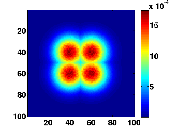
Figure 4: Spatial positions of different 2D Gaussian functions for four sources. The left map shows the case without overlap ($d=6\sigma_{Map}$) and the right map shows the case with maximum overlap ($d=2\sigma_{Map}$). The intermediate cases ($d=5\sigma_{Map}$, $d=4\sigma_{Map}$ and $d=3\sigma_{Map}$) are not represented.

5.2 Estimation of number of sources

We tested the method used to estimate the number of sources (Section 3.1) on our 45 synthetic data cubes. For each of them, we found the true number of sources of the mixture. These results are unambiguous because the difference between $\lambda_{(L)}$ and $\lambda_{(L+1)}$ clearly appears. We can easily differenciate the two parts $\Omega_{S}$ and $\Omega_{E}$ on each curve of ordered eigenvalues. We illustrate the method for a mixture of 4 sources in Fig. 5. A “break” is clearly observed in the curve of ordered eigenvalues at index $r=5$. The number of sources identified by the method is correct, $L=r-1=4$.

Figure 5: Example of identification of number of sources for a synthetic mixture of four sources with SNR = 10 dB and $d=2\sigma_{Map}$.

5.3 Unmixing

5.3.1 Quality measures

We now present the performance of the different BSS methods introduced in Section 4: MC-NMF, SpaceCorr, MASS and their hybrid versions. To study the behavior of these methods, we apply them to the 45 synthetic cubes. We use two measures of error as performance criteria, one for maps and the other for spectra. The Normalized Root Mean Square Error (NRMSE) defines the error of estimated maps:

$$NRMSE_{\ell}=\frac{\|s_{\ell}-\hat{s}_{\ell}\|}{\|s_{\ell}\|}.$$ (35)

The spectral angle mapper (SAM) normalized root mean square error

defines the error of estimated spectra. This usual measurement in hyperspectral imaging for Earth observation is defined as the angle formed by two spectra:

$$SAM_{\ell}=\operatorname*{arccos}\left(\frac{a_{\ell}^{T}\hat{a}_{\ell}}{\|a_{\ell}\|.\|\hat{a}_{\ell}\|}\right).$$ (36)

The Monte Carlo analysis associated with the NMF makes it possible to define the spread of the solutions given by each of the $K$ runs of the NMF. For each estimated source, we construct the envelope giving the spread of the solutions around the most probable solution according to (16). The amplitude of the envelope is normalized by the maximum intensity in order to obtain the error bars as a percentage of the maximum intensity. This normalization is arbitrary and makes it possible to express the spread of the MC-NMF independently from the spectral intensity. We first denote as $\text{NMCEB}_{\ell}$ (for Normalized Monte Carlo Error Bar) the normalized error associated with the $\ell^{th}$ elementary spectrum:

$$\text{NMCEB}_{\ell}(n)=\frac{\alpha_{\ell}(n)+\beta_{\ell}(n)}{U_{\ell}}\qquad\forall n\in\{1,\ldots,N\},$$ (37)

where $U_{\ell}=\underset{n}{\operatorname*{max}}\{a_{\ell}(n)\}$ is the maximal intensity of the $\ell^{th}$ elementary spectrum. To quantify the total spread of MC-NMF solutions for a data cube, the above parameter is then maximized along the spectral axis:

$$\text{NMCEB}_{\ell}^{\text{max}}=\operatorname*{max}_{n}\{\text{NMCEB}_{\ell}(n)\}.$$ (38)

For clarity, we hereafter detail two examples of mixtures of four sources with SNR = 20 dB. The results for other mixtures with an SNR of 10, 20, or 30 dB lead to the same conclusions and are available in Appendix B. More specifically, some additional tests with a very low SNR (1, 3, or 5 dB) are also reported in Appendix B.8 for the preferred two methods. Their relative merits are then modified as expected, as compared to the above cases involving significantly higher SNRs.

5.3.2 Results

The first example is a case of a highly sparse mixture ($d=6\sigma_{Map}$), whose map is shown in the leftmost part of Fig. 4. The second example concerns a weakly sparse mixture ($d=2\sigma_{Map}$), whose map is shown in the rightmost part of Fig. 4. Again to simplify the figures, we present only one component but the results are similar for the remaining 3 components.

The results in the most sparse case are given in Fig. 6 and Fig. 7. The first figure illustrates the performance of the MC-NMF, SpaceCorr or MASS methods used alone and the second figure shows the results of the resulting four hybrid methods. Similarly, the results in the least sparse case are given in Fig. 8 and Fig. 9.

In the most sparse case, the results of MC-NMF are consistent with the previously highlighted drawbacks. On the one hand, we note a variability of results which leads to significant error bars. On the other hand, the estimated spectrum yields a significant error. This corresponds to an overestimation of the maximum intensity of the spectrum and an underestimation of the width of the beam. Furthermore, we observe the residual presence of close sources, visible on the map of Fig. 6 (a).

The SpaceCorr and MASS methods provided excellent results (see Fig. 6 (b-c)), which is consistent with the theory. This first case is in the optimal conditions of use of the method, since many adjacent observed pixels are single-source.

Regarding hybrid methods, we observe a significant reduction of the error bars in agreement with the objective of these methods. However when MC-NMF is initialized with the previously estimated spectra (see Fig. 7 (a-c)), we find on the estimated spectra the same inaccuracy as with MC-NMF used alone (overestimation of the maximum intensity and underestimation of the width of the beam). Initialization with previously estimated abundance maps gives the best performance, with very similar results for the two algorithms based on this approach (Fig. 7 (b-d)). For the SC-NMF-Map and MASS-NMF-Map methods, there is performance improvement, as compared respectively with SpaceCorr and MASS used alone, although the latter two methods are already excellent.

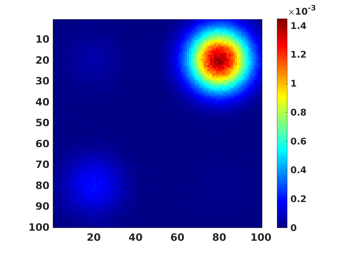
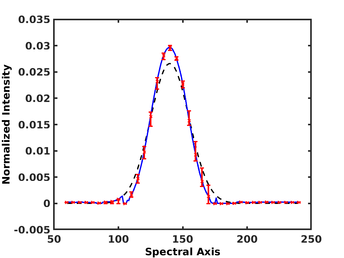
(a) MC-NMF (20.81%, 0.107 rad)
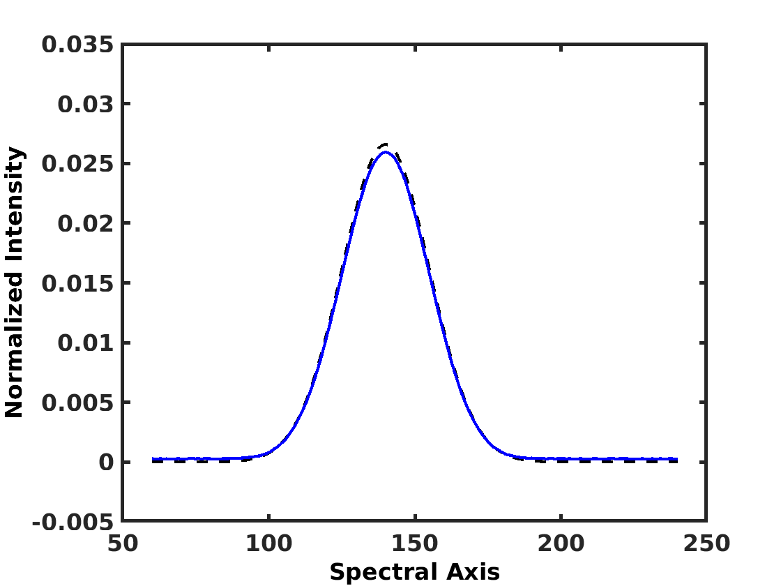
(b) SpaceCorr (2.69%, 0.019 rad)
(c) MASS (2.07%, 0.019 rad)

Figure 6: Results of the decomposition for the MC-NMF, SpaceCorr, and MASS methods in the most sparse case ($d=6\sigma_{Map}$). Estimated spectrum is in blue, actual spectrum is in black dashes, and red error bars give the spread of the solutions of MC-NMF. Each subfigure caption contains the name of the considered BSS method, followed by the NRMSE of the estimated abundance map and the SAM of the estimated spectrum (see (35) and (36)). This also applies to the subsequent figures.

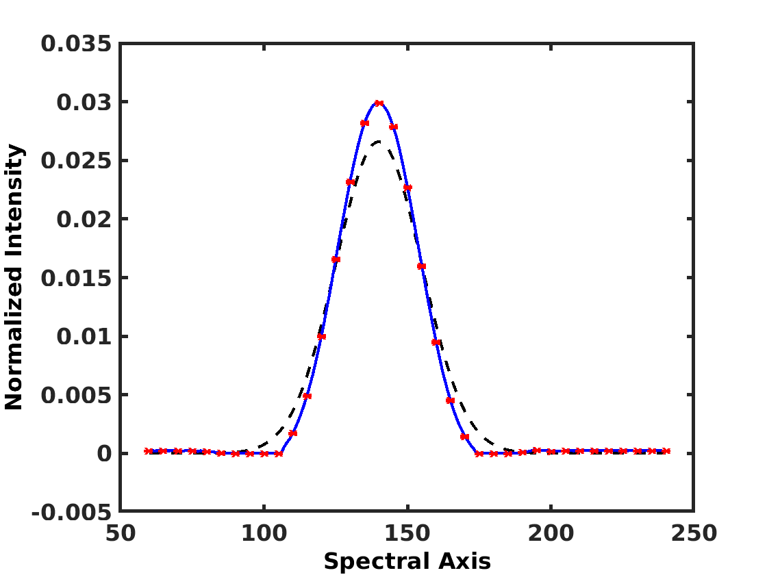
(a) SC-NMF-Spec (21.47%, 0.102 rad)
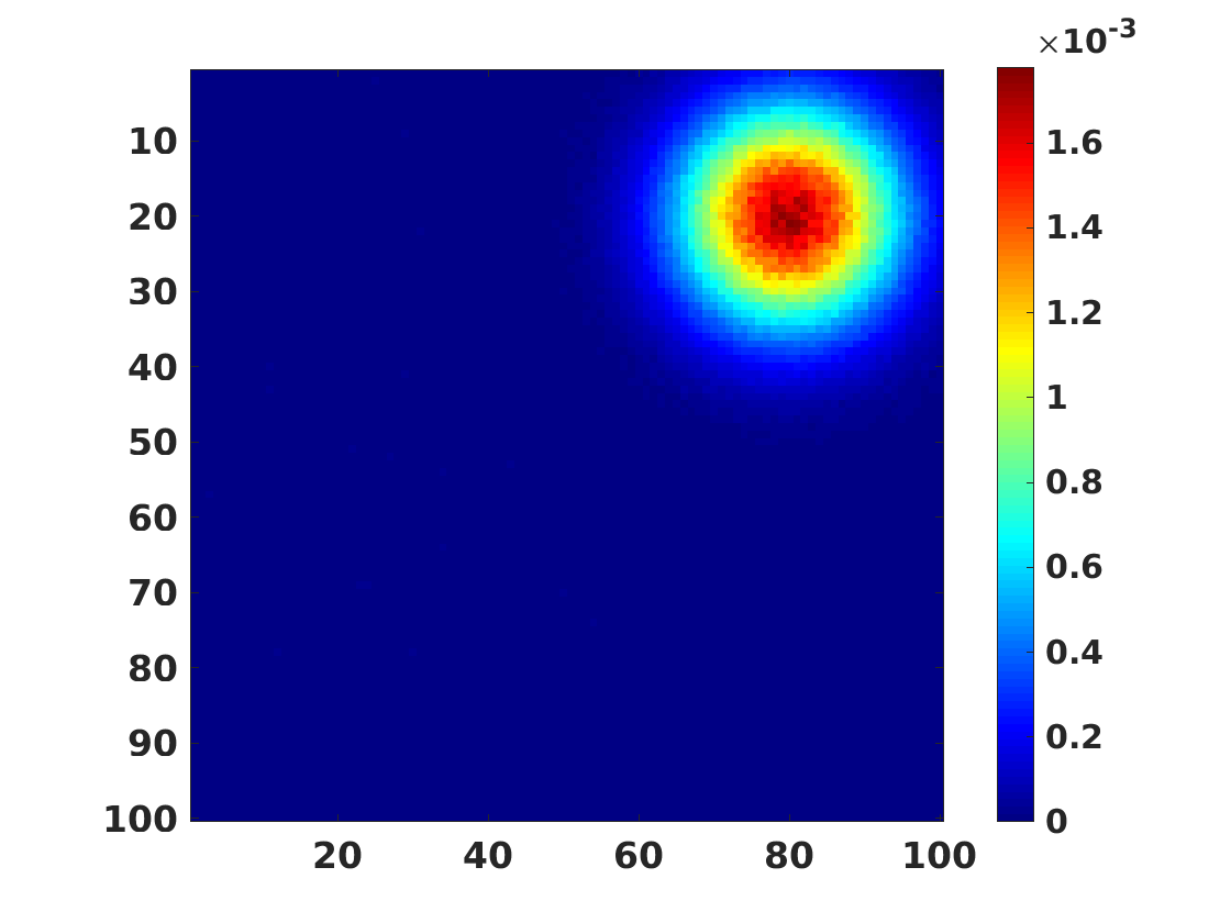
(b) SC-NMF-Map (2.13%, 0.016 rad)
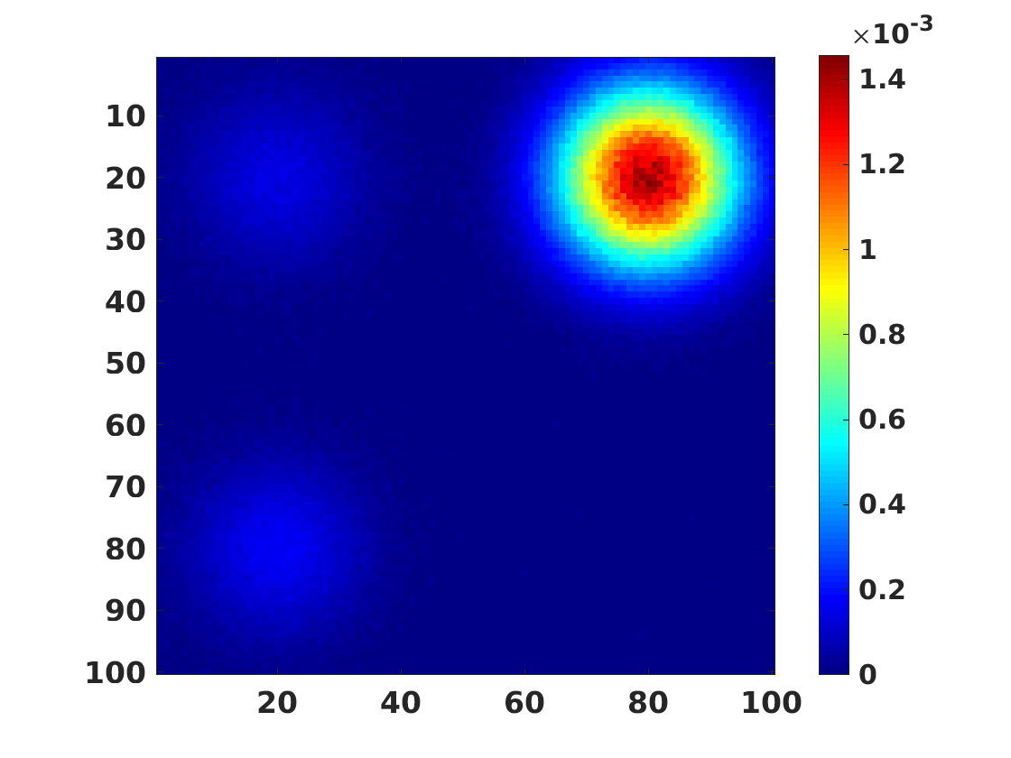
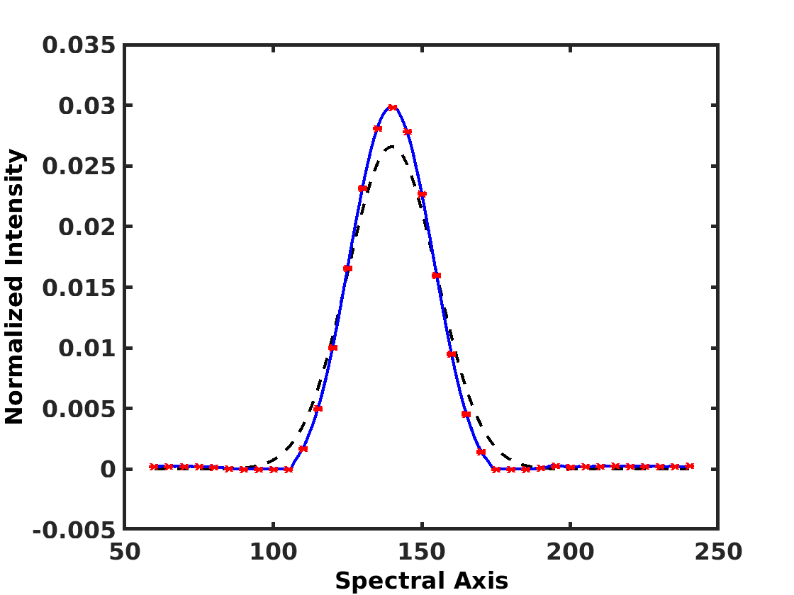
(c) MASS-NMF-Spec (21.32%, 0.101 rad)
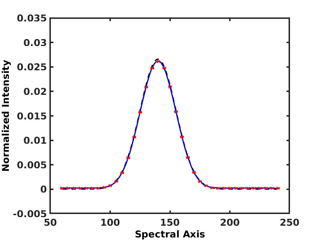
(d) MASS-NMF-Map (1.95%, 0.016 rad)

Figure 7: Results of the decomposition for hybrid methods in the most sparse case ($d=6\sigma_{Map}$). Estimated spectrum is in blue, actual spectrum is in black dashes, and red error bars give the spread of the solutions.

In the least sparse case, MC-NMF provides estimated spectra which have almost the same accuracy as in the most sparse case (see Fig. 8 (a)). We observe the same deformation of the estimated beam, a large spread of the solutions and a residual source on the abundance map.

This time, SpaceCorr does not provide satisfactory results. Indeed, abundance maps seem to give a good approximation of ground truth but estimated spectra are contaminated by the presence of the other spectral components (see Fig. 8 (b)). This contamination leads to an underestimation of the peak of intensity, the loss of the symmetry of the beam as well as a positioning error for the maximum of intensity on the spectral axis. This perturbation is explained by the fact that there are few single-source zones in the cube. Furthermore, the detection step is sensitive to the fixed threshold for selection of the best single-source zones. Depending on the choice of the threshold, some “quasi-single-source” zones may turn out to be used to estimate the columns of the mixing matrix $A$.

In this case, the MASS method yields a better estimate than SpaceCorr (see Fig. 8 (c)), thanks to its ability to operate with single-source pixels, instead of complete single-source spatial zones. The obtained spatial source is correctly located and is circular (unlike with the SpaceCorr method, where it was slightly deformed). The estimated spectrum is better than that estimated by SpaceCorr, however it is slightly noisy because of the sensitivity of MASS to the high noise level (see Appendix B).

Here again, all four hybrid methods significantly reduce the error bars, as compared with applying MC-NMF alone. Initializations with SpaceCorr results (Fig. 9 (a-b)) improve the results of SpaceCorr without completely removing the residue of other spectral components (i.e., the estimated spectrum is still somewhat asymmetric). In addition, we observe again that when MC-NMF is initialized with the spectra (Fig. 9 (a-c)), we obtain the estimated spectra with the same inaccuracy as with the MC-NMF used alone. The initialization with MASS results (Fig. 9 (c-d)) improves the results of MASS by removing the residual noise of the estimated spectrum. As an overall result, the initialization of MC-NMF with the abundance maps provided by MASS (see Fig. 9 (d), including a 6.08% NRSME and a 0.034 rad SAM) gives the best performance in this difficult case of weakly sparse and highly noisy data.

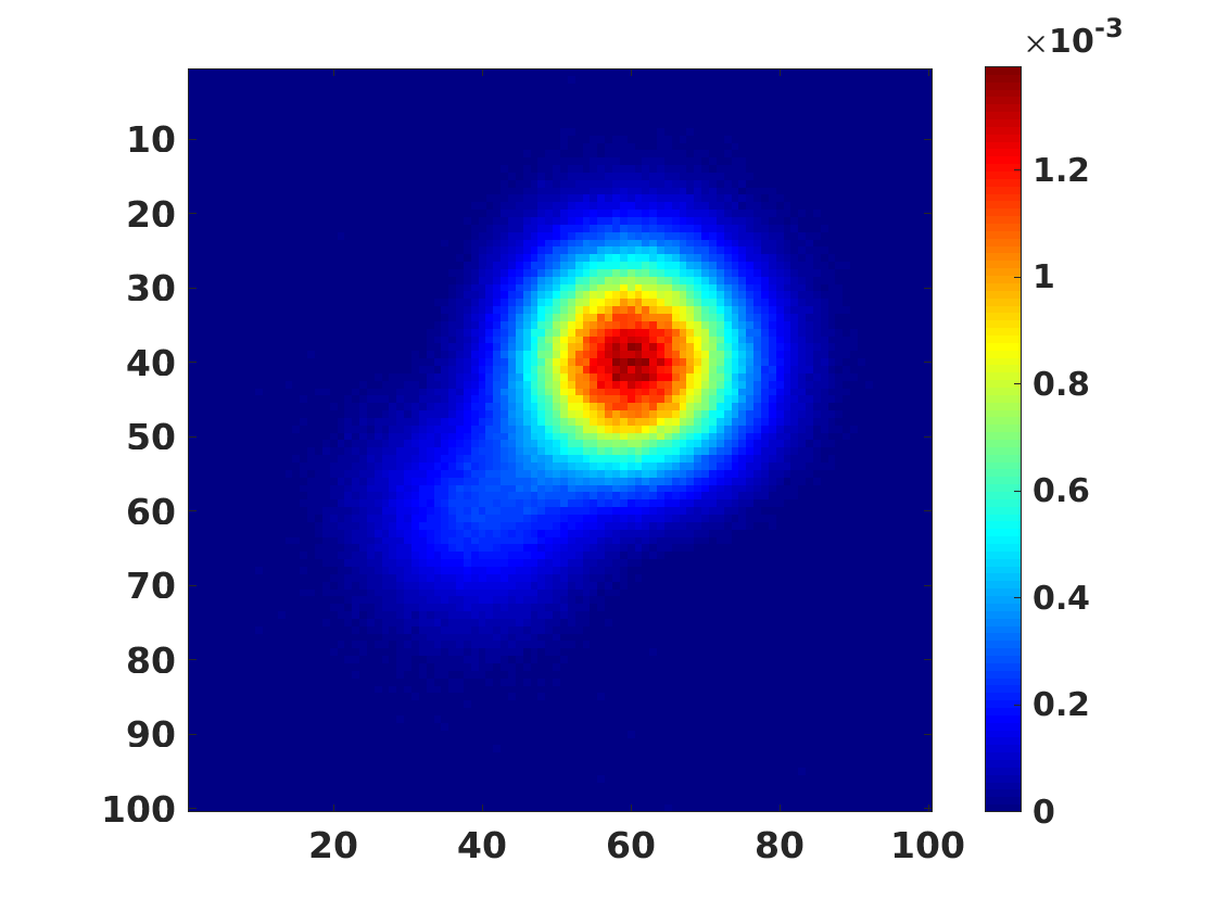
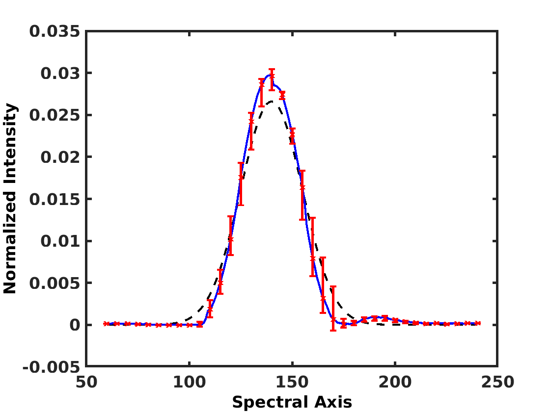
(a) MC-NMF (23.63%, 0.126 rad)
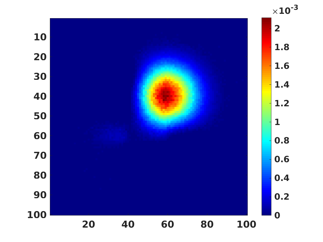
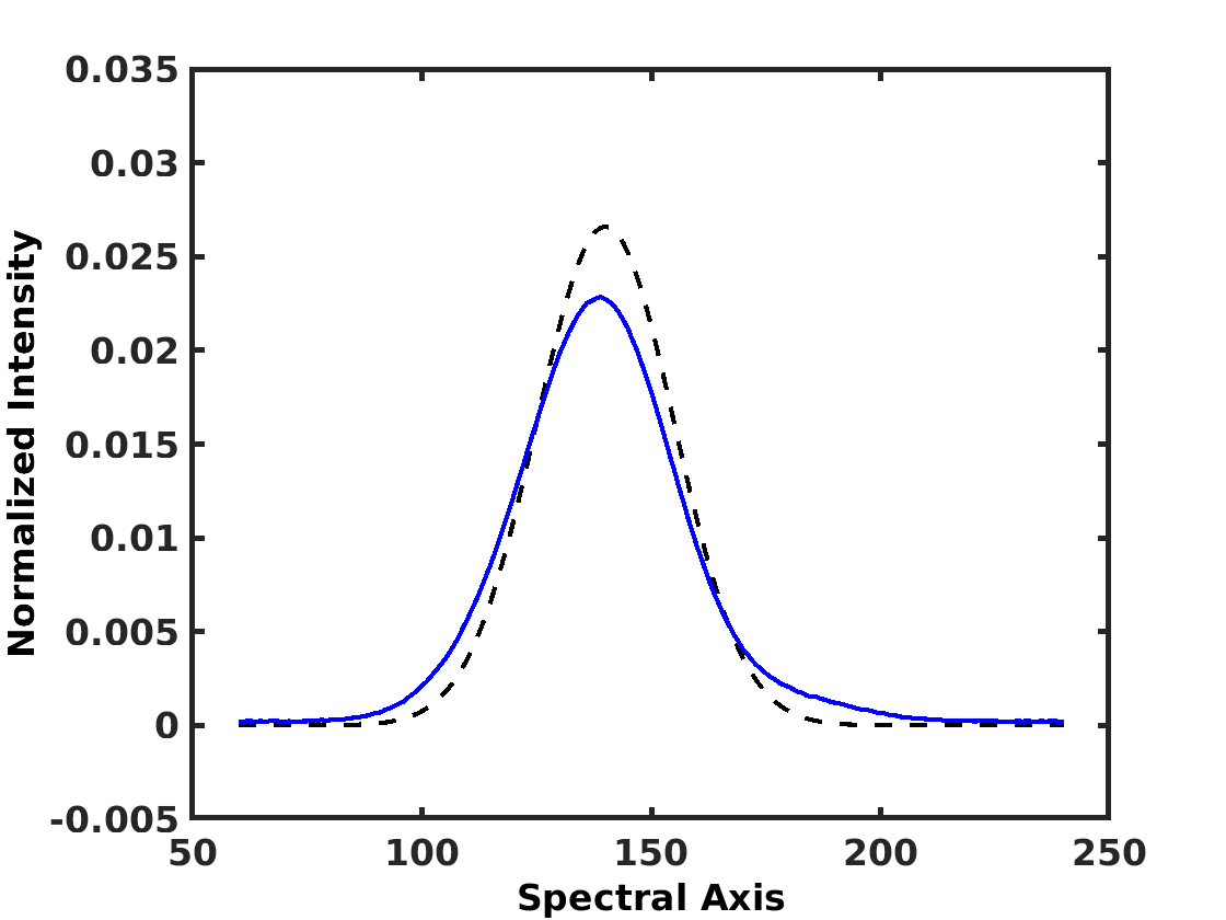
(b) SpaceCorr (19.67%, 0.122 rad)
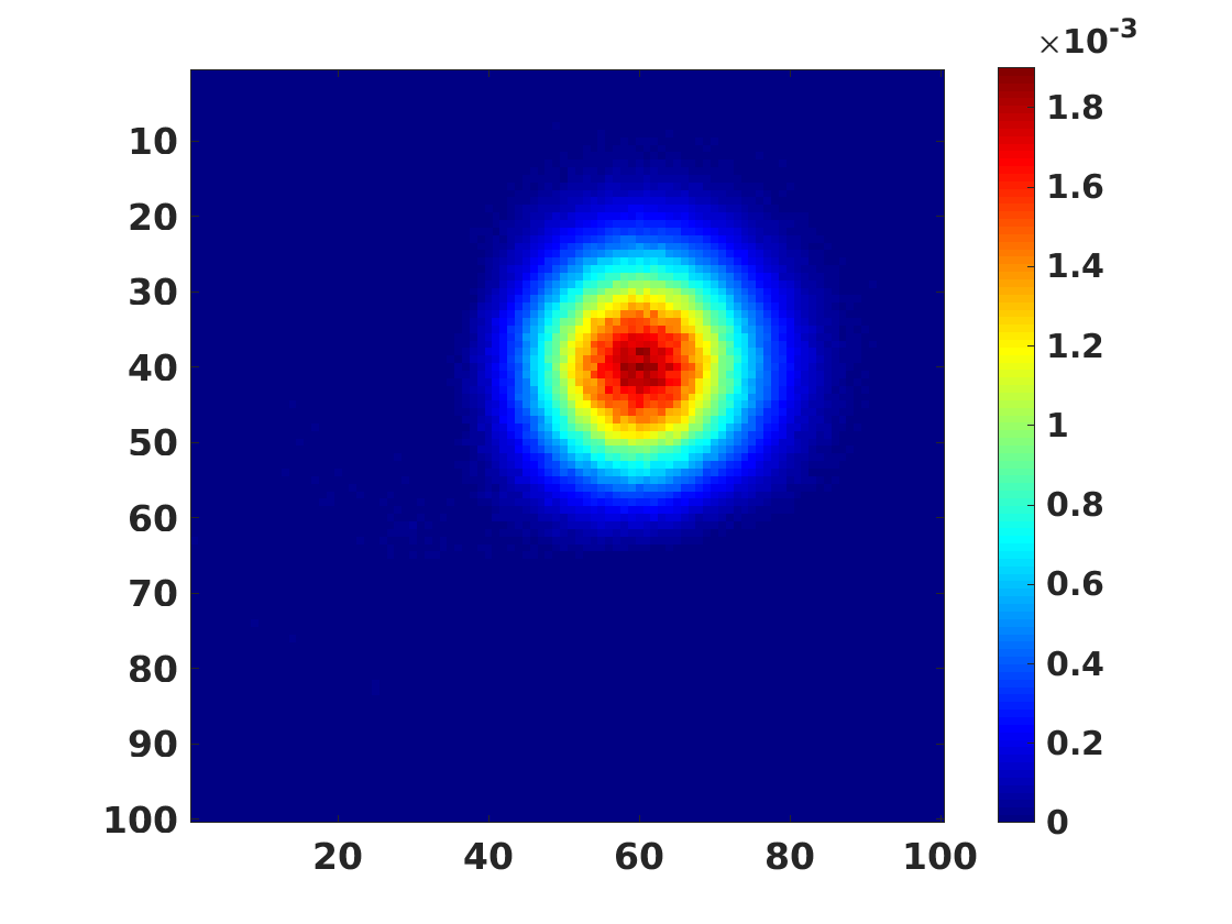
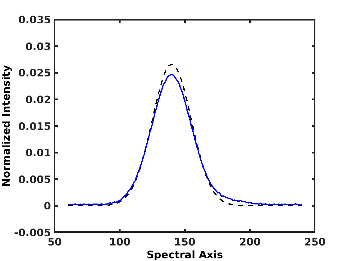
(c) MASS (8.84%, 0.051 rad)

Figure 8: Results of the decomposition for the MC-NMF, SpaceCorr and MASS methods in the least sparse case ($d=2\sigma_{Map}$). Estimated spectrum is in blue, actual spectrum is in black dashes, and red error bars give the spread of the solutions of MC-NMF.

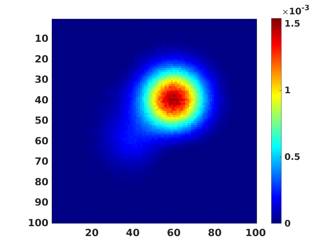
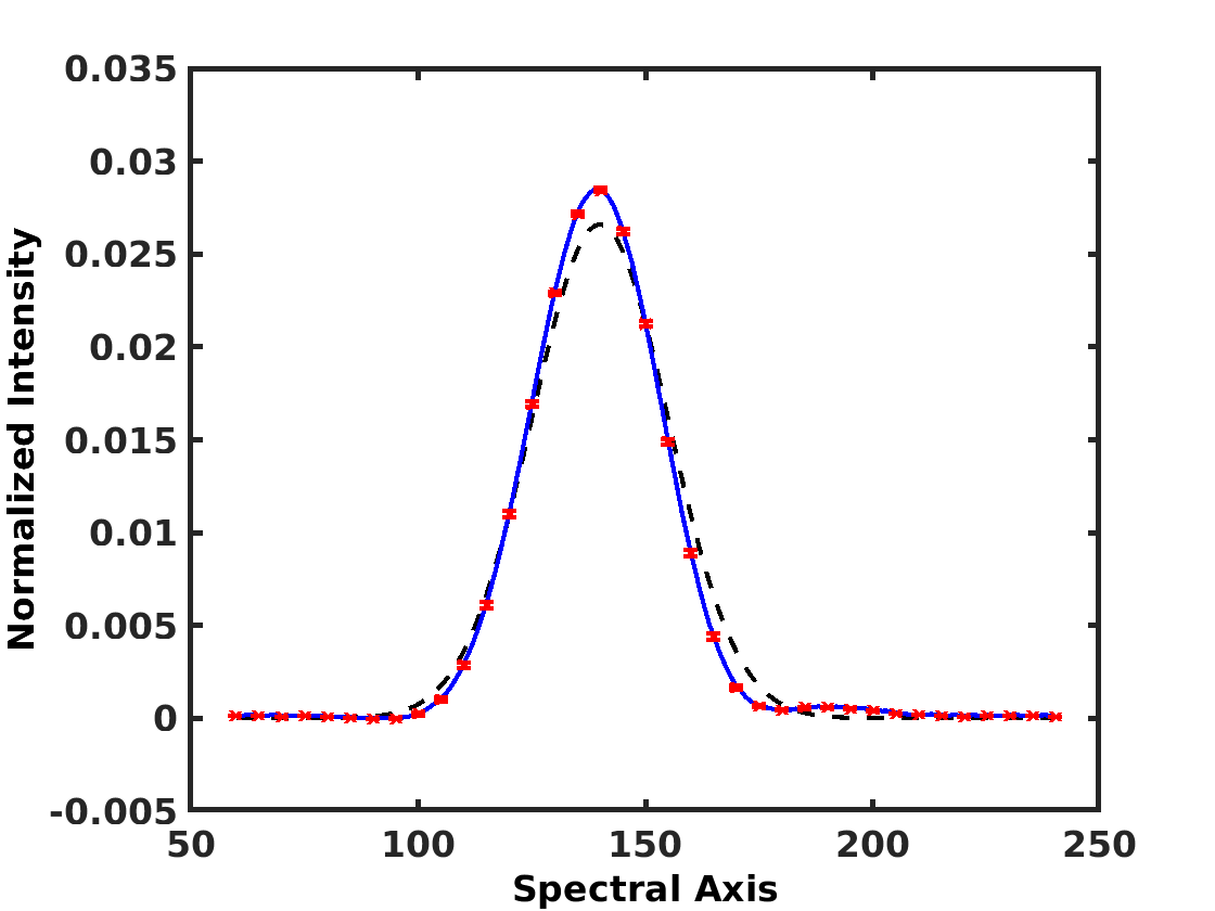
(a) SC-NMF-Spec (16.20%, 0.082 rad)
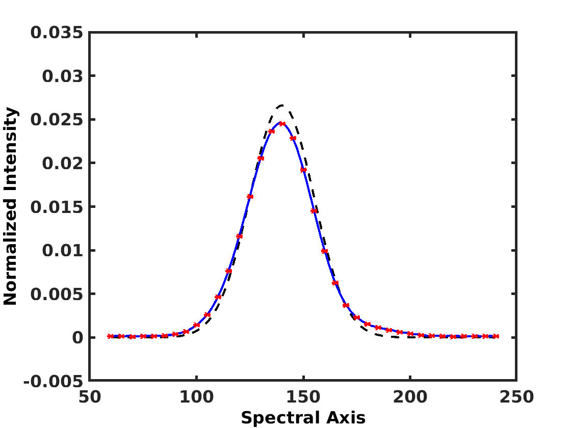
(b) SC-NMF-Map (10.37%, 0.065 rad)
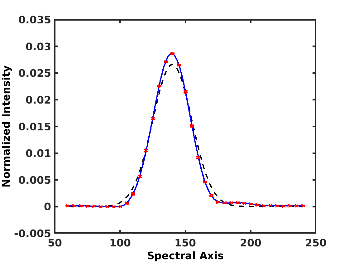
(c) MASS-NMF-Spec (16.69%, 0.080 rad)
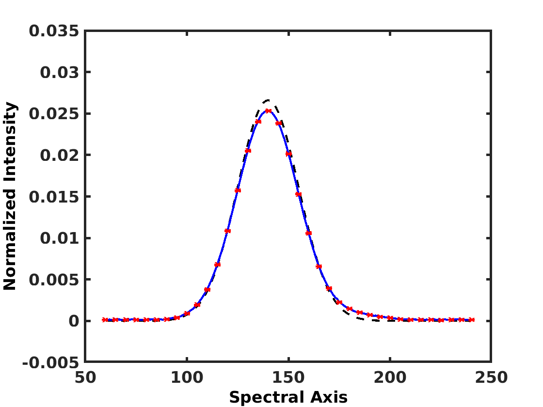
(d) MASS-NMF-Map (6.08%, 0.034 rad)

Figure 9: Results of the decomposition for hybrid methods in the least sparse case ($d=2\sigma_{Map}$). Estimated spectrum is in blue, actual spectrum is in black dashes and red error bars give the spread of the solutions.

$d$	$criterion$	MC-NMF	SpaceCorr	SC-NMF-Spec	SC-NMF-Map	MASS	MASS-NMF-Spec	MASS-NMF-Map
$6\sigma_{Map}$	NRMSE	15.59 %	3.05 %	16.52 %	2.58 %	3.58 %	16.60 %	3.30 %
	SAM (rad)	0.077	0.019	0.089	0.015	0.030	0.090	0.018
	$\text{NMCEB}^{\text{max}}$	13.65 %	-	0.69 %	2.58e-3 %	-	0.70 %	4.92e-3 %
$2\sigma_{Map}$	NRMSE	18.25 %	20.59 %	11.76 %	11.67 %	10.37 %	12.82 %	8.36 %
	SAM (rad)	0.084	0.145	0.061	0.082	0.077	0.057	0.050
	$\text{NMCEB}^{\text{max}}$	22.25 %	-	1.51 %	8.93e-2 %	-	1.24 %	0.72 %

Table 2: Performance obtained with the considered methods for a cube containing 4 sources with a 20 dB SNR. Results in bold identify the cases when hybrid methods improve performance, as compared with the MC-NMF, SpaceCorr or MASS methods used alone. The underlined results identify the best results obtained for each of the two cubes respectively corresponding to $d=6{\color[rgb]{0,0,0}\sigma_{Map}}$ and $d=2{\color[rgb]{0,0,0}\sigma_{Map}}$.

5.3.3 Summary of the results

To conclude on the synthetic tests, we group in Table 2 the performances obtained by the different methods for the cube containing four sources with an SNR of 20 dB. The reported performance values are averaged over all four components and 100 noise realizations.

First, the four hybrid methods presented here highly improve the spread of the solutions given by MC-NMF used alone. This point is the first interest to use hybrid methods.

With regard to the decomposition quality achieved by the SC-NMF and MASS-NMF hybrid methods, the synthetic data tests show that the Map initialization provides better results than the “Spec” one in almost all cases, whatever the considered source sparsity. Therefore, as an overall result, Map initialization is the preferred option. The only exception to that trend is that SC-NMF-Spec yields a better result than SC-NMF-Map in terms of SAM for low-sparsity sources.

The last point to be specified in these tests is the choice of the method used to initialize MC-NMF with the “Map” initialization selected above, namely SpaceCorr or MASS. The results of Table 2 refine those derived above from Fig. 6 to 9, with a much better statistical confidence, because they are here averaged over all sources and 100 noise realizations, instead of considering only one source and one noise realization in the above figures. The results of Table 2, in terms of NRSME and SAM, thus show that SC-NMF-Map yields slightly better performance than MASS-NMF-Map in the most sparse case, whereas MASS-NMF-Map provides significantly better performance in the least sparse case. This result is not surprising, because SC-NMF-Map sets more stringent constraints on source sparsity, but is expected to yield somewhat better performance when these constraints are made (thanks to the data averaging that it peforms over analysis zones). In a “blind configuration”, i.e. when the degree of sparsity of the sources is not known, the preferred method for the overall set of data considered here is MASS-NMF-Map because, as compared with SC-NMF-Map, it is globally better in the sense that it may yield significantly better or only slightly worse performance, depending on sparsity.

It should be noted at this stage that we suspect that what favors MASS-NMF-Map is related to the dimension of the data cube, i.e. that this latter method performs better here because there are, in the synthetic data, more points spatially than spectrally (i.e. 10⁴ spatial points vs 300 spectral points). Hence, by initializing with SCA results the matrix that contains the largest number of points, MASS-NMF-Map provides a better solution. On the contrary, in the recent study by Foschino et al. (2019), the authors have found that MASS-NMF-Spec performs better. In their specific case case, the (real) data contain only 31 spatial positions and 6799 spectral points. This suggests that the general recommendation is to use the version of the method (Spec or Map) that initializes the largest number of points in the NMF with SCA results.

6 Conclusion and future work

In this paper, we proposed different versions of Blind Source Separation methods for astronomical hyperspectral data. Our approach was to combine two well-known classes of methods, namely NMF and Sparse SCA, in order to leverage their respective advantages while compensating their disadvantages. We developed several hybrid methods based on this principle, depending on the considered SCA algorithm (SpaceCorr or MASS) and depending whether that SCA algorithm is used to set the initial values of spectra or abundances then updated by our Monte-Carlo version of NMF, called MC-NMF. In particular, our MASS-NMF-Map hybrid method, based on initializing MC-NMF with the abundance maps provided by MASS, yields a quasi-unique solution to the decomposition of a synthetic hyperspectral data cube, with an average error (summarized in Table 2) which is always better, and often much better, than that of the MC-NMF, SpaceCorr and MASS methods used separately. Our various tests on simulated data also show robustness to additive white noise. Since the initialization of NMF with SCA methods was here shown to yield encouraging results, our future work will especially aim at developing SCA methods with lower sparsity constraints, in order to further extend the domain where the resulting hybrid SCA-NMF methods apply. A first application of the MASS-NMF-Spec method presented in this paper on real data is presented in Foschino et al. (2019) and shows the potential of such methods for current and future hyperspectral datasets.

Appendix A Data processing methods

A.1 K-means method

K-means is a standard unsupervised classification method (Theodoridis & Koutroumbas (2009)) which aims to partition a set of $N$ vectors $x$ into $k$ sets $\{\sigma_{1},\sigma_{2},\ldots,\sigma_{k}\}$. Within each set $\sigma_{i}$, a measure of dissimilarity $d$ between vectors $x\in\sigma_{i}$ and cluster representative $c_{i}$ is minimized. The cluster representative $c_{i}$ (or centroid) is the mean vector in the cluster $\sigma_{i}$. In our case, the measure of dissimilarity is 1 minus the correlation between $x\in\sigma_{i}$ and $c_{i}$:

$$d(x,{\color[rgb]{0,0,0}c_{i}})=1-corr(x,{\color[rgb]{0,0,0}c_{i}}).$$ (39)

Performing clustering then amounts to minimizing the following objective function:

$$J(U,C)=\sum\limits_{i=1}^{k}\sum\limits_{j=1}^{N}U_{ij}d(x_{j},c_{i}),$$ (40)

where $C$ is the matrix of centroids $c_{i}$ and $U$ is a partition matrix such that $U_{ij}=1$ if $x_{j}\in\sigma_{i}$ and $0$ otherwise. Moreover, each vector belongs to a single cluster (hard clustering):

$$\sum\limits_{i=1}^{k}U_{ij}=1\qquad j\in\{1,\ldots,N\}.$$ (41)

The K-means algorithm is defined as follows:

Input : A set of vectors $x$, the number of cluster $k$.

Output : A partition matrix $U$, a set of centroids $C$.

1 begin

       Choose arbitrary initial $C_{0}$ for the centroids;

        /* In practice, $k$ vectors $x$, randomly selected */

2       $U\leftarrow 0$;

3       repeat

             /* Update clusters */

4             for $j=1$ to $N$ do

5                   Determine the closest representative, say $c_{i}$, for $x_{j}$ in the sense of $d$;

6                   $U_{ij}\leftarrow 1$;

7                  

8             end for

            /* Update centroids */

9             for $i=1$ to $k$ do

10                   Determine $c_{i}$ as the mean of the vectors $x\in\sigma_{i}$;

11                  

12             end for

13            

14      until no change in $c_{i}$’s occurs between two successive iterations;

15 end

16

Algorithm 1 K-means

However, a well-known drawback of this algorithm is its sensitivity to the initialization, the final centroids depending on the choice of initial cluster representatives $c_{i}$. But for our two clustering steps, a manual initialization is possible and avoids this drawback:

• As part of Monte-Carlo analysis of NMF (Section 4.1), we use as initial centroids $C_{0}$ the $L$ spectra estimated by the first Monte-Carlo trial.

• As part of the estimation step of SpaceCorr (Section 4.2), we use as initial centroids $C_{0}$ the $L$ farthest spectra in the sense of the measure $d$ (see Eq. (39)), among the potential columns of the matrix $\hat{A}$.

A.2 Parzen kernel method

The estimation by Parzen kernel or Parzen windows (Theodoridis & Koutroumbas (2009); Silverman (1998)) is a parametric method for estimating the probability density function (pdf) of a random variable at any point of its support $\Omega$. Let $(x_{1},x_{2},\ldots,x_{N})$ be an independent and identically distributed sample of a random variable $X$ with an unknown pdf $f$. Its kernel density estimator is:

$$\hat{f}(x)=\frac{1}{Nh}\sum\limits_{i=1}^{N}K\left(\frac{x_{i}-x}{h}\right)\qquad x\in\Omega,$$ (42)

where $K$ is a kernel, i.e., a smooth nonnegative function that integrates to one, and $h>0$ is a smoothing parameter called the bandwidth (or width of window). In our case, we use as the kernel the standard normalized Gaussian function (zero expectation and unit standard deviation):

$$K(x)=\frac{1}{\sqrt{2\pi}}e^{\left(-\frac{1}{2}x^{2}\right)}.$$ (43)

The bandwidth $h$ of the kernel is a free parameter which exhibits a strong influence on the resulting estimate. In the case of a Gaussian kernel, it can be shown (Silverman (1998)) that the optimal choice for $h$ is:

$$h=\left(\frac{4\hat{\sigma}^{5}}{3N}\right)^{\frac{1}{5}}\approx 1.06\hat{\sigma}N^{-\frac{1}{5}},$$ (44)

where $\hat{\sigma}$ is the sample standard deviation. The Parzen kernel algorithm is defined as follows:

Input : Sample points $X$.

Output : The estimated pdf $\hat{f}$, a support $\Omega$ covering the range of the data.

1 begin

       Compute $h$;

        /* According to (44) */

       Define the support such that $\Omega=[min(X),max(X)]$;

        /* In practice, Card $(\Omega)=100$ */

2       for $k=1$ to Card$(\Omega)$ do

             Compute the estimate of $\hat{f}(\Omega_{k})$;

              /* According to (42) */

3            

4       end for

5      

6 end

7

Algorithm 2 Parzen Kernel

Appendix B Additional test results

The next figures show the performance of the methods applied to all cubes. The SAM and the NRMSE values presented in the following figures are obtained by averaging these measurements for each method over all 100 noise realizations. We also provide error bars which define the standard deviation over all noise realizations. Each such NMCEB spread measurement is obtained in two stages. Firstly, for each source, the average spectrum and the average envelope are defined over all noise realizations. In a second step, we identify the maximum, first along the spectral axis ($n$) for a given source ($\ell$), and then with respect to all sources.

To summarize, we associate with each method a first figure composed of six frames arranged in two rows and three columns. The first row gives the SAM and the second the NRMSE. The first column concerns cubes containing 2 sources, the middle one containing 4 sources and the last one containing 6 sources. Within each frame, the $x$ axis gives the distance $d$ defining the overlap between the spatial sources, from $d=6{\color[rgb]{0,0,0}\sigma_{Map}}$ down to $d=2{\color[rgb]{0,0,0}\sigma_{Map}}$. In Sections B.1 to B.7, inside each such frame, the three curves respectively correspond to each of the three main noise levels tested in this study: blue for 30 dB Signal to Noise Ratio (SNR), red for 20 dB and black for 10 dB. Similarly, in Section B.8, inside each frame, the three curves respectively correspond to each of the three additional tested low SNRs: blue for 5 dB, red for 3 dB and black for 1 dB. For the MC-NMF method and the hybrid methods, we also provide a second figure, consisting of 3 frames giving the NMCEB maximum for each of the 45 cubes.

In conclusion, all of these tests and illustrations aim to quantify several phenomena. First, evaluate the impact of the noise level and the distance between the sources on the performance of the methods. Next, quantify the contribution of hybrid methods compared to the MC-NMF, SpaceCorr and MASS methods used alone. The study of the error bars of the Monte-Carlo analysis associated with the NMF makes it possible to evaluate the spread of the solutions as a function of the noise level, the sparsity of the sources and the initialization.

B.1 Results with MC-NMF

The performance of the MC-NMF method is shown in Fig. 10 and 11. We will first consider the cases involving four or six sources. The performance of MC-NMF then has a low sensitivity to the distance $d$, i.e. to the source joint sparsity. Similarly, the number of sources is a criterion having a relatively limited effect on the performance of MC-NMF in our simulations. On the contrary, the noise level has a significant effect on the quality of the solutions given by MC-NMF (although the noiseless case does not give ideal results). It should be noted that the amplitude of the error bars of MC-NMF depends on all the tested parameters (degree of sparsity, number of sources and noise level). The variability of MC-NMF solutions is often substantial and the goal of hybrid methods is to reduce this variability.

We will now focus on the case of 2 sources. For distances ranging from $d=6\sigma_{Map}$ down to $d=3\sigma_{Map}$ (or at least $4{\color[rgb]{0,0,0}\sigma_{Map}}$), the same comments as those provided above for 4 or 6 sources still apply, as expected. On the contrary, further decreasing $d$ to $d=2{\color[rgb]{0,0,0}\sigma_{Map}}$ results in an unexpected behavior: the SAM and NRMSE values then strongly decrease. In other words, in this situation when the sources become more mixed, performance improves. Several causes can lead to this result, such as the presence of noise, the symmetry of the maps, the great similarity of the spectra or the number of iterations of the NMF, although all these features also apply to the cubes containing 4 or 6 sources. To analyze the influence of such features on the shape of the cost function to be minimized and thus on performance, we performed the following additional tests for 2 sources:

• No noise in the mixtures.

• Deleting the normalization of the spectra at each iteration of the NMF.

• Random switching of columns of $X$.

• Avoiding the symmetry of abundance maps by deforming a 2D Gaussian.

• Avoiding the similarity of the spectra by changing the nature of the function simulating the line (triangle or square function).

• Fixed number of iterations of the NMF.

• Deleting the observed spectra having a power lower than 90% of the maximal observed power.

Each of these tests led to the same, unexpected, trend as that observed in the first column of Fig 10. On the contrary, the expected behavior was observed in the following additional test, where the sparsity of the sources was varied. The abundance maps simulated by 2D Gaussians are replaced by a matrix $S$ of dimension $2\times 100$ whose elements are drawn with a uniform distribution between 0.5 and 1. The first 25 elements of the first row are multiplied by a coefficient $\alpha$. The elements 26 to 50 of the second row are also multiplied by the same coefficient $\alpha$. Thus, depending on the value of $\alpha$, we simulate more or less sparsity in the data. In this test, we observe a decrease of the performance of MC-NMF when $\alpha$ increases, i.e. when the source sparsity decreases, as expected. Finally, we performed tests for all the cubes (as well as for the hybrid methods), where we further decreased the distance $d$ to $d=1{\color[rgb]{0,0,0}\sigma_{Map}}$, which corresponds to very low sparsity. The SAM and NMRSE then considerably increase, which corresponds to the expected behavior of BSS methods. The above-defined unexpected behavior is therefore only observed in the specific case involving 2 sources and the intermediate distance $d=2\sigma_{Map}$, and it could be further analyzed in future work.

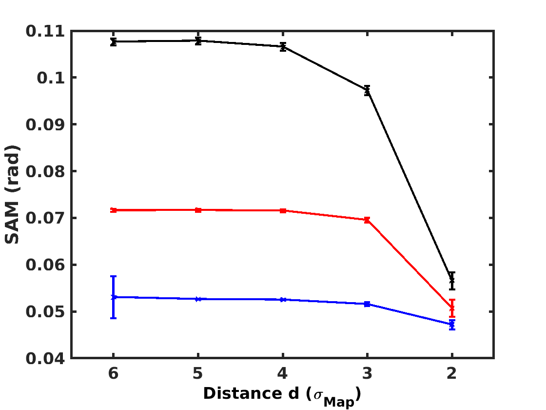
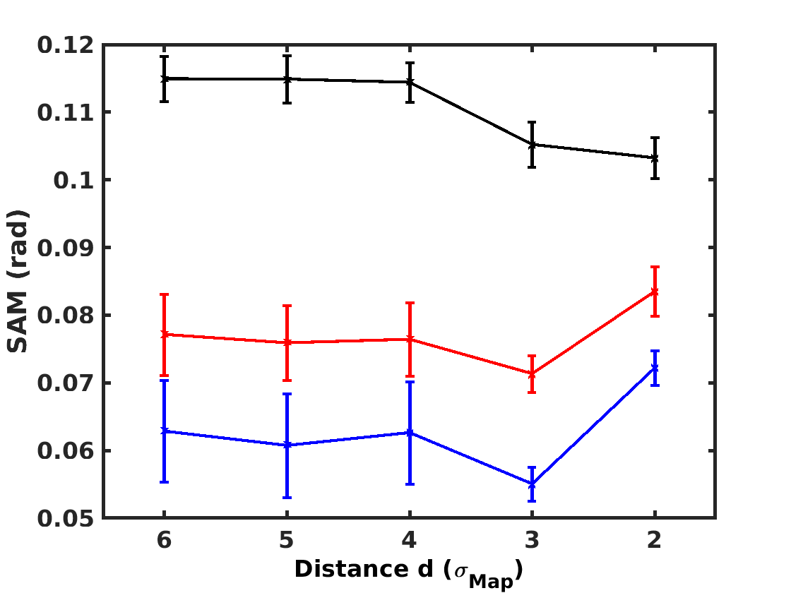
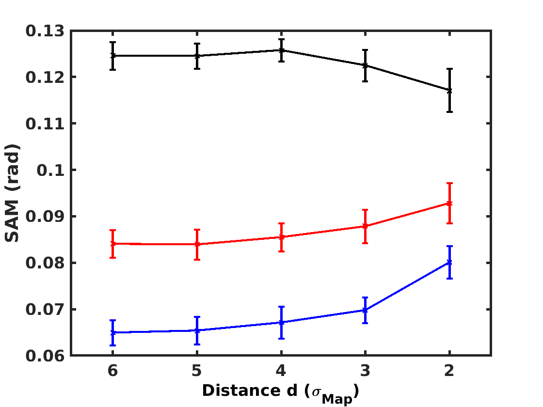
2 sources	4 sources	6 sources

Figure 10: Performances achieved by MC-NMF on the 45 synthetic cubes for 100 realizations of noise with an SNR of 30 dB (in blue), 20 dB (in red), and 10 dB (in black). The error bars give the standard deviation over the 100 realizations of noise.

2 sources	4 sources	6 sources

Figure 11: Spread (NMCEB) of the solutions of MC-NMF obtained on the 45 synthetic cubes with 100 realizations of noise.

B.2 Results with SpaceCorr

The performance of the SpaceCorr method is shown in Fig. 12. This method gives excellent results if the data are sparse enough, i.e., if there are a sufficient number of single-source zones, which here corresponds to a large enough distance $d$. We also note that SpaceCorr is not very sensitive to the number of sources. Its (limited) sensitivity is at least due to the fact that the number of sources over the considered fixed spatial area may have an influence on the degree of source sparsity in terms of available single-source zones. Finally, we emphasize that SpaceCorr is relatively robust to noise in data. The presence of residuals in the estimates of the least sparse cases is due to the small number of single-source zones per source in the data. In addition, the step of detection of the single-source zones is sensitive to the choice of the threshold used to select the best single-source zones. Depending on this threshold, almost single-source zones may be used to estimate the columns of the mixing matrix, which yields contributions from other sources. However, the sensitivity of the method to the choice of this parameter will be attenuated by hybridization with MC-NMF.

2 sources	4 sources	6 sources

Figure 12: Performances achieved by SpaceCorr on the 45 synthetic cubes for 100 realizations of noise with an SNR of 30 dB (in blue), 20 dB (in red), and 10 dB (in black). The error bars give the standard deviation over the 100 realizations of noise.

B.3 Results with SC-NMF-Spec

Whatever the number of sources, the SC-NMF-Spec hybrid version (Fig. 13) yields results with the same trend as that obtained by MC-NMF used alone for two sources (Fig. 10, leftmost column). Moreover, when considering two sources for both methods, they yield similar estimation errors for given sparsity and noise level. Besides, SC-NMF-Spec results in a much lower spread (Fig. 14) than MC-NMF (Fig. 11), especially for four or six sources. This property is the main goal of hybridization.

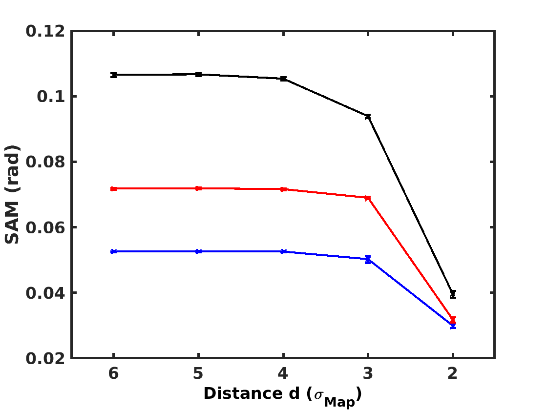
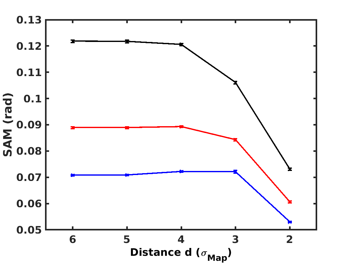
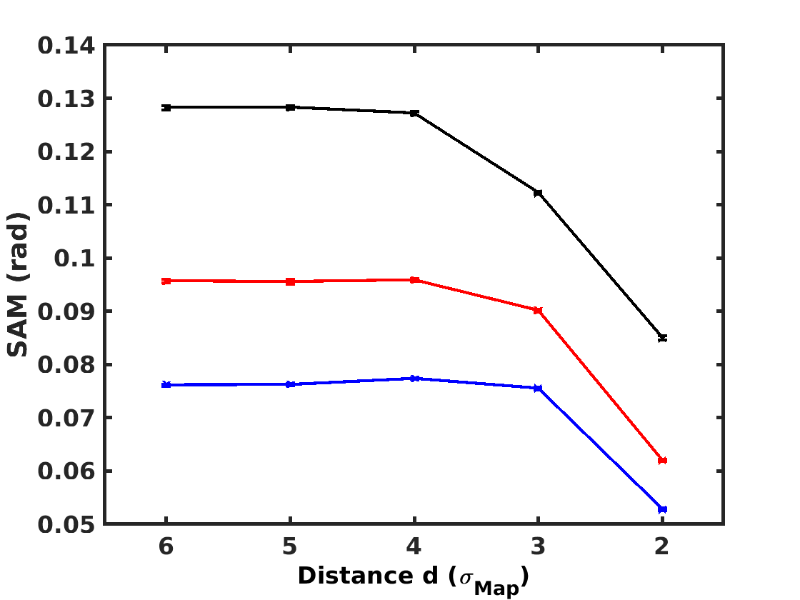
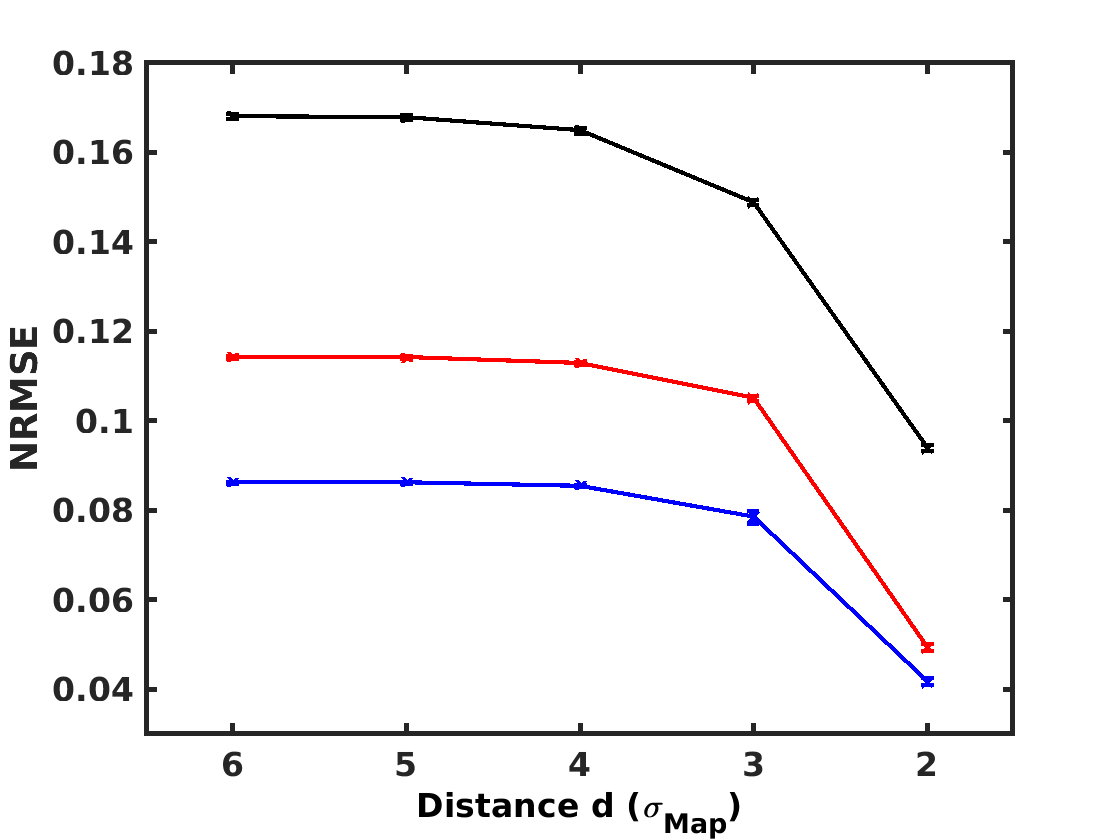
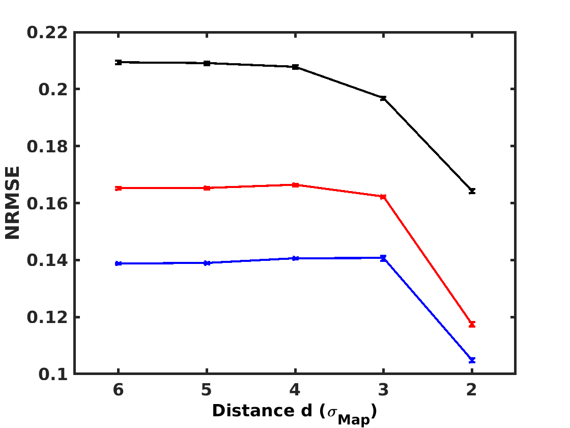
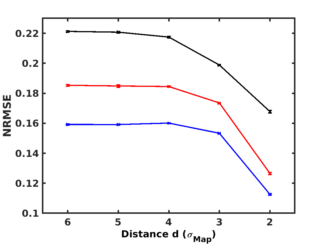
2 sources	4 sources	6 sources

Figure 13: Performances achieved by SC-NMF-Spec on the 45 synthetic cubes for 100 realizations of noise with an SNR of 30 dB (in blue), 20 dB (in red), and 10 dB (in black). The error bars give the standard deviation over the 100 realizations of noise.

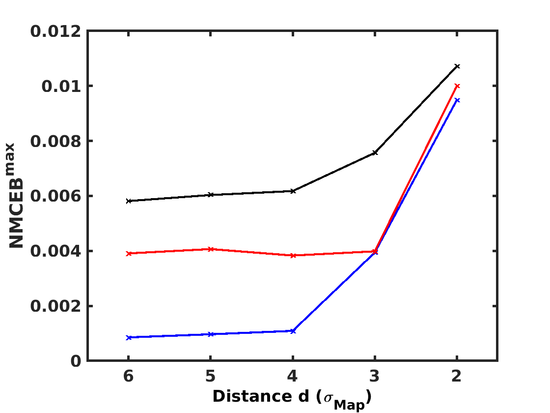
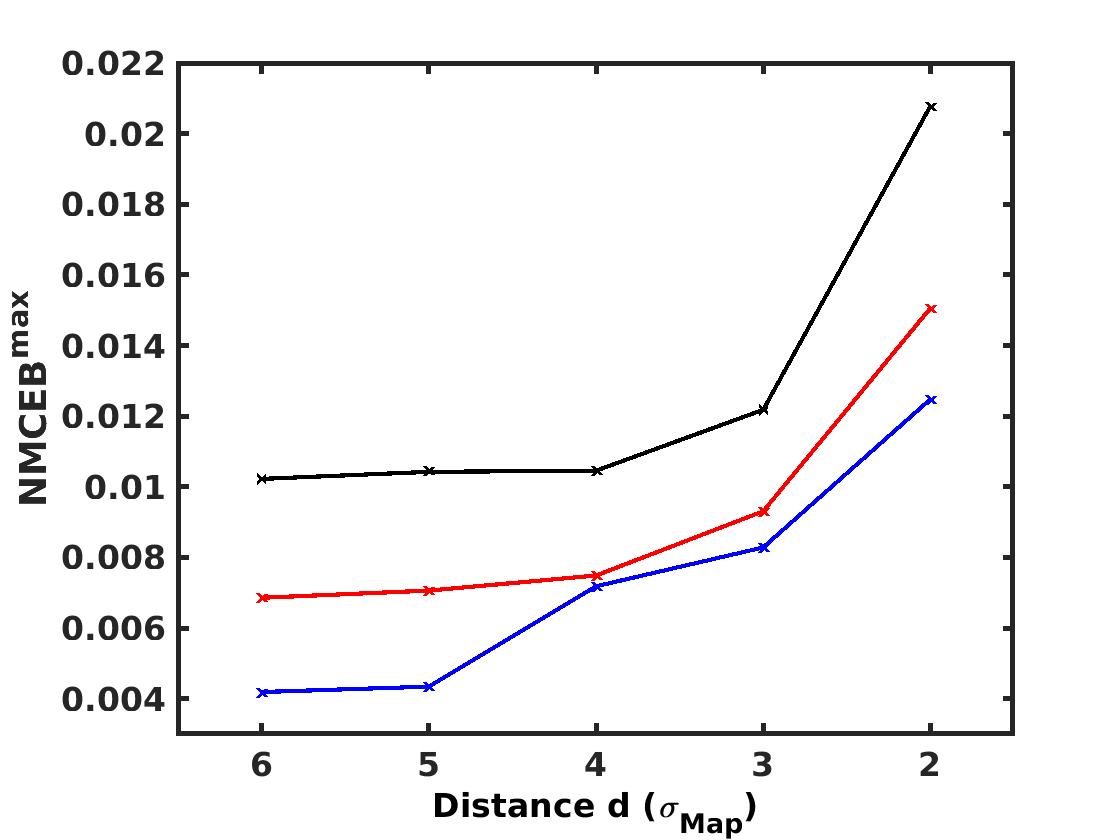
2 sources	4 sources	6 sources

Figure 14: Spread (NMCEB) of the solutions of SC-NMF-Spec obtained on the 45 synthetic cubes with 100 realizations of noise.

B.4 Results with SC-NMF-Map

The SC-NMF-Map hybrid version (Fig. 15) yields results with the same trend as that obtained by SpaceCorr used alone (Fig. 12), whatever the number of sources. Moreover, SC-NMF-Map results in significantly lower estimation errors, especially in difficult cases. The spread of the results given by SC-NMF-Map (Fig. 16) becomes negligible, with an improvement of an order of magnitude over the amplitude of the error bars of the SC-NMF-Spec hybrid version.

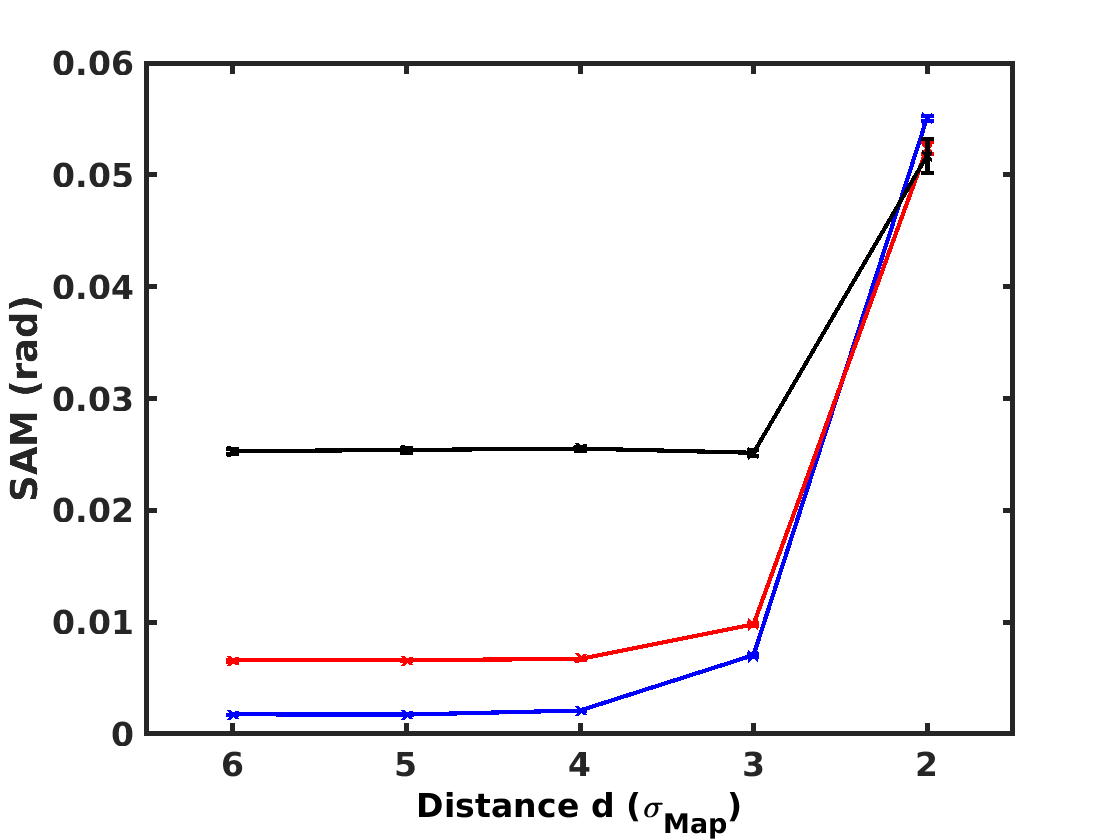
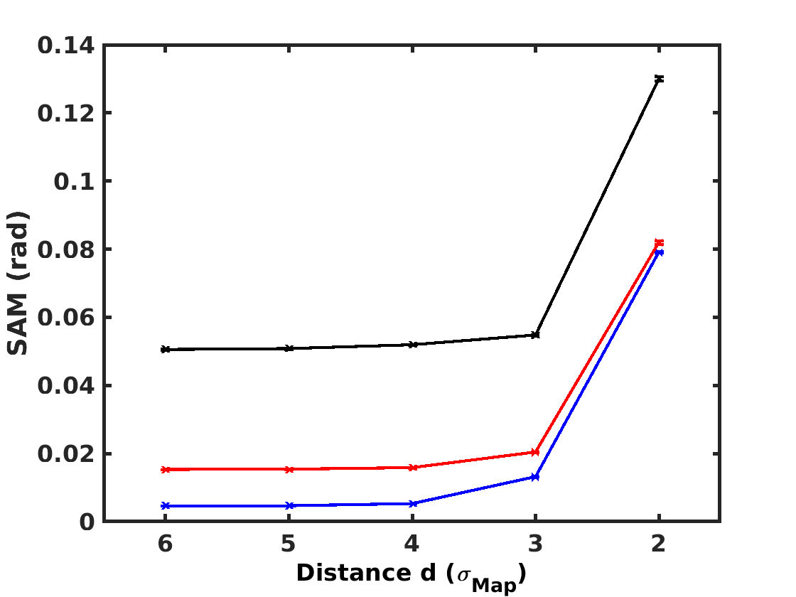
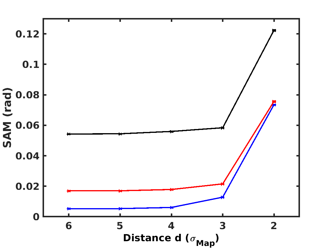
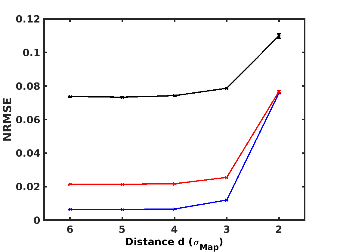
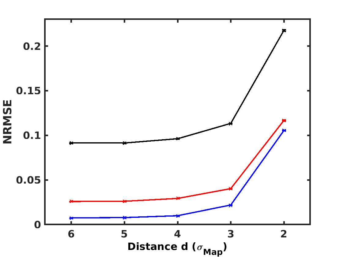
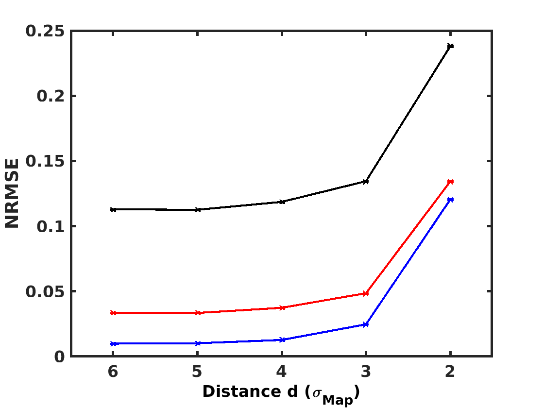
2 sources	4 sources	6 sources

Figure 15: Performances achieved by SC-NMF-Map on the 45 synthetic cubes for 100 realizations of noise with an SNR of 30 dB (in blue), 20 dB (in red), and 10 dB (in black). The error bars give the standard deviation over the 100 realizations of noise.

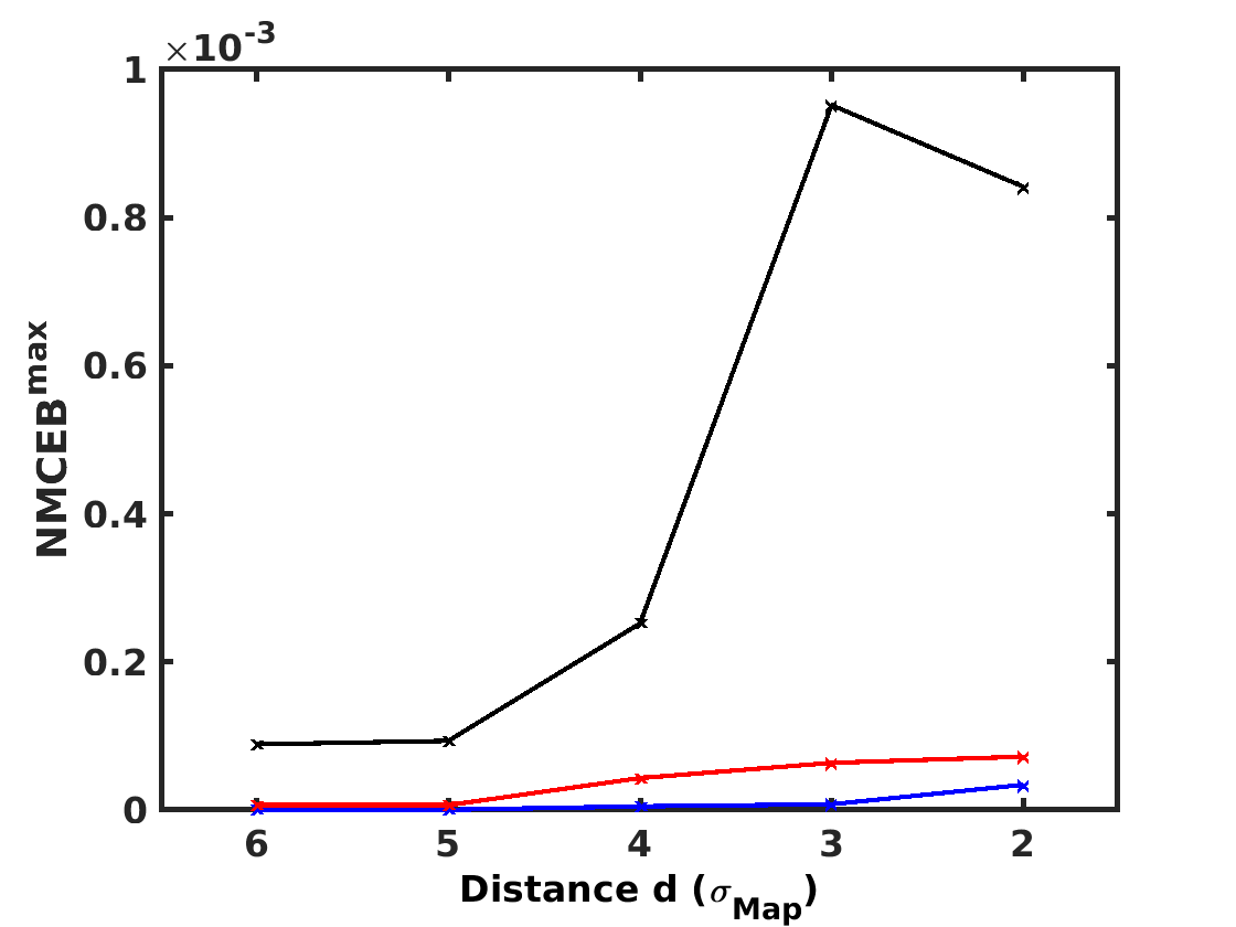
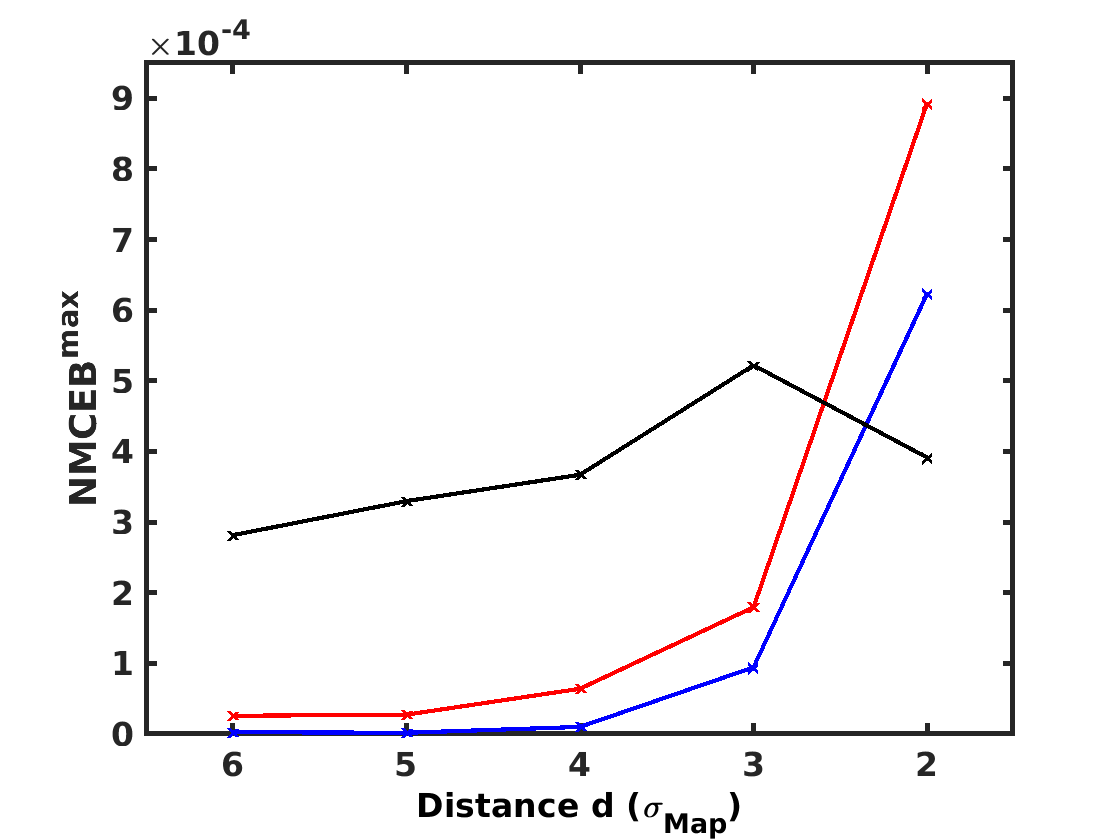
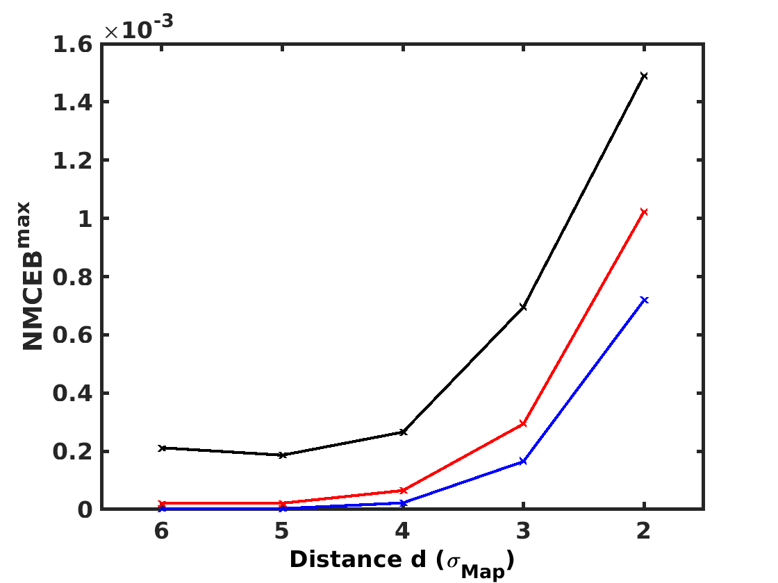
2 sources	4 sources	6 sources

Figure 16: Spread (NMCEB) of the solutions of SC-NMF-Map obtained on the 45 synthetic cubes with 100 realizations of noise.

B.5 Results with MASS

MASS gives excellent results in the case of sufficiently sparse data and in the presence of a reasonable noise level (20 or 30 dB SNR). It is further noted that for mixtures of two or four sources, the results are correct even under the least favorable conditions of sparsity, again with an SNR of 20 or 30 dB.

The main disadvantage highlighted by the synthetic data tests is the sensitivity of the method to the high level of noise. Indeed, the performances for the mixtures with a 10 dB SNR are weak, even under optimal conditions of sparsity. This sensitivity comes from the structure of the method that performs the estimation of the mixing matrix by directly selecting the columns from the observed vectors. The introduction of a tolerance angle in this selection has an effect at reasonable noise levels but becomes less effective at higher noise levels. In addition, reducing the tolerance threshold would allow greater robustness to noise, to the detriment of component separation. Non single-source observations would then be used in the estimation of the columns of the mixing matrix. The sensitivity of MASS to the noise level can be mitigated by hybridization with MC-NMF.

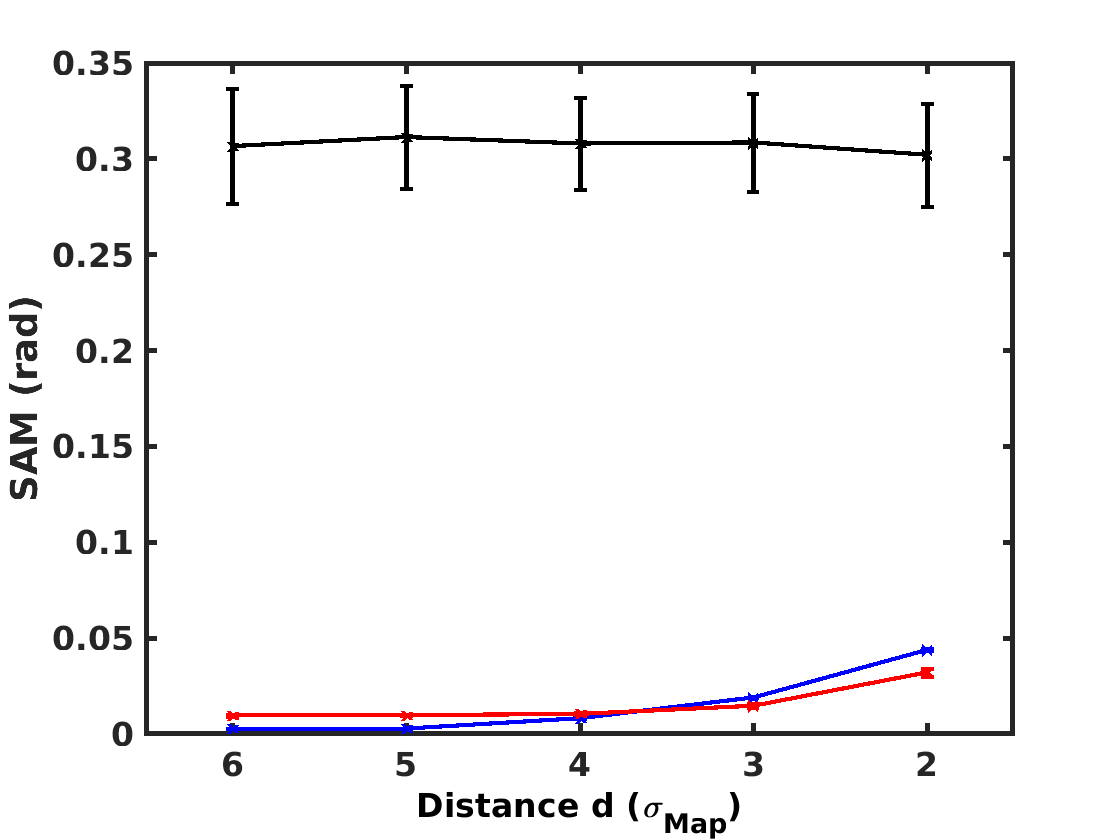
2 sources	4 sources	6 sources

Figure 17: Performances achieved by MASS on the 45 synthetic cubes for 100 realizations of noise with an SNR of 30 dB (in blue), 20 dB (in red), and 10 dB (in black). The error bars give the standard deviation over the 100 realizations of noise.

B.6 Results with MASS-NMF-Spec

The MASS-NMF-Spec hybrid version (Fig. 18) yields the same trends as those obtained by SC-NMF-Spec (Fig. 13). In comparison with the MASS method alone, the main advantage is an overall improvement of the performance criteria for mixtures with 10 dB SNR. The MASS method used alone in this configuration gave unsatisfactory results. They are markedly improved during hybridization with MC-NMF. Finally, we note the major decrease in the spread of the solutions given by MASS-NMF-Spec (Fig. 19) compared to that encountered with the MC-NMF (Fig. 11), especially for four or six sources. The error bars encountered here are of the same order of magnitude as those obtained with SC-NMF-Spec (Fig. 14).

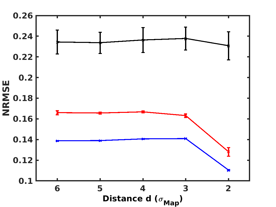
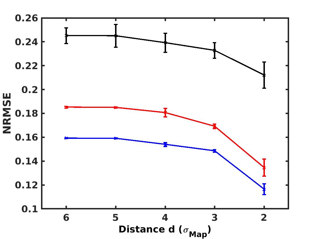
2 sources	4 sources	6 sources

Figure 18: Performances achieved by MASS-NMF-Spec on the 45 synthetic cubes for 100 realizations of noise with an SNR of 30 dB (in blue), 20 dB (in red), and 10 dB (in black). The error bars give the standard deviation over the 100 realizations of noise.

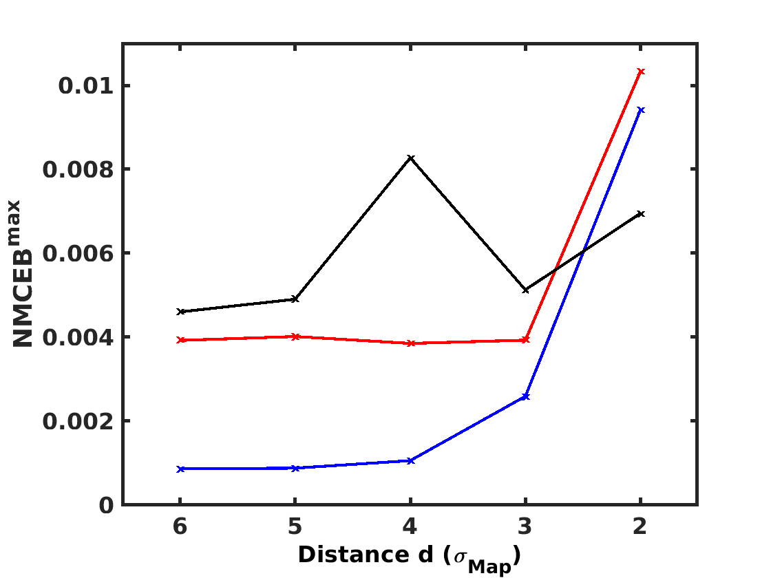
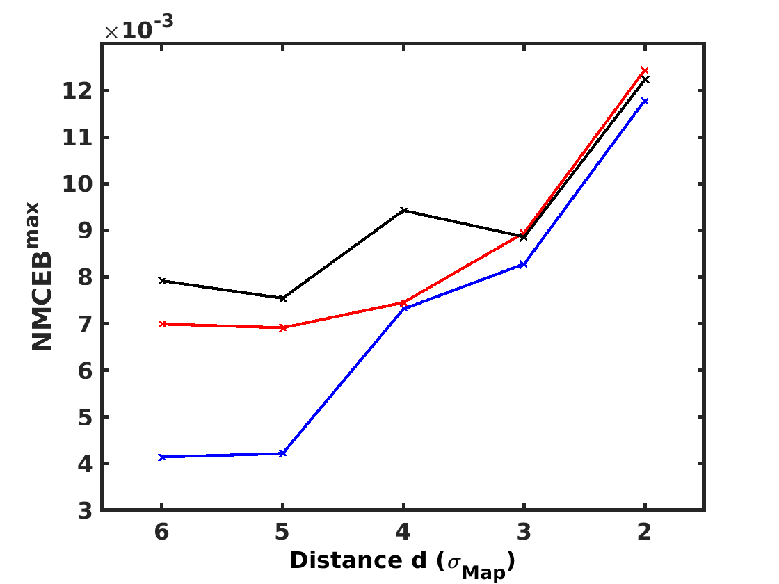
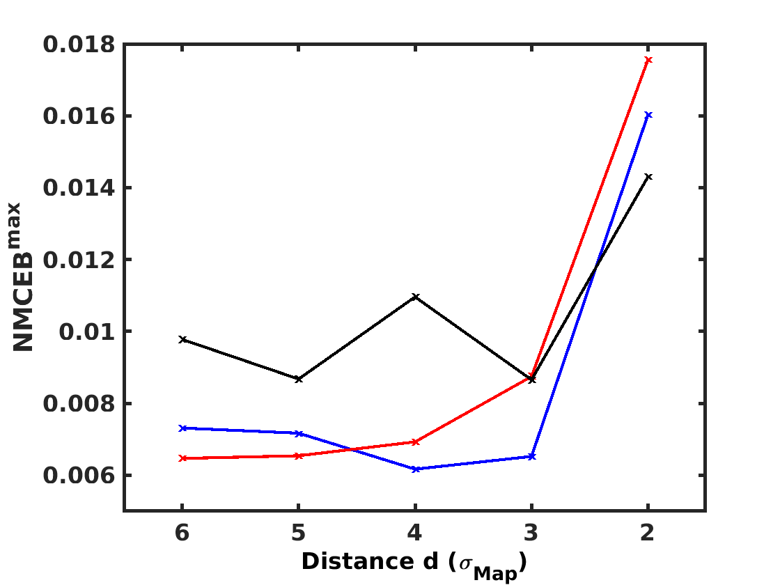
2 sources	4 sources	6 sources

Figure 19: Spread (NMCEB) of the solutions of MASS-NMF-Spec obtained on the 45 synthetic cubes with 100 realizations of noise.

B.7 Results with MASS-NMF-Map

The MASS-NMF-Map hybrid version (Fig. 20) yields the same trends as those obtained by MASS used alone (Fig. 17). Again, there is a noticeable improvement in performance for mixtures with a 10 dB SNR compared to MASS used alone, as well as a clear improvement in the spread of the solutions (Fig. 21) compared to that obtained with the MC-NMF method alone (Fig. 11), especially for 4 or 6 sources.

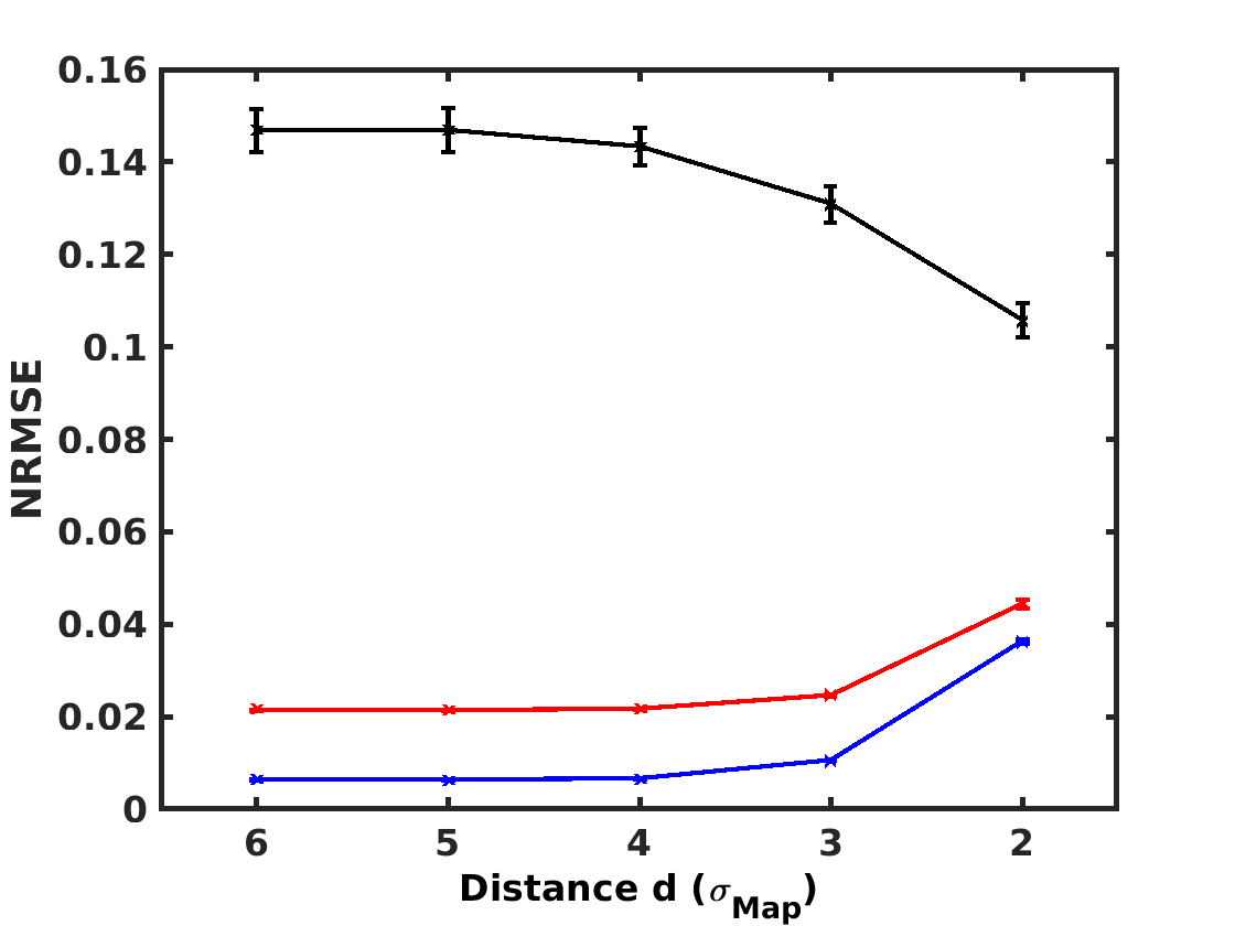
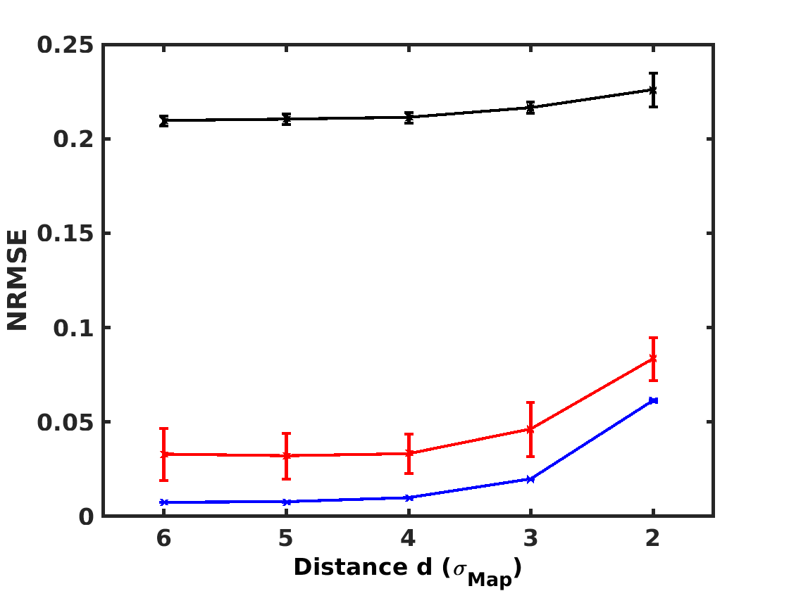
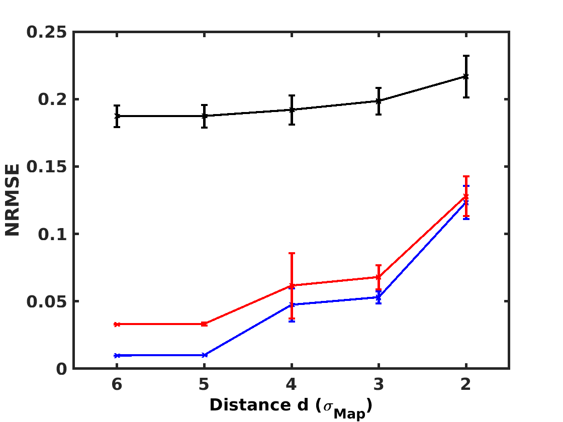
2 sources	4 sources	6 sources

Figure 20: Performances achieved by MASS-NMF-Map on the 45 synthetic cubes for 100 realizations of noise with an SNR of 30 dB (in blue), 20 dB (in red), and 10 dB (in black). The error bars give the standard deviation over the 100 realizations of noise.

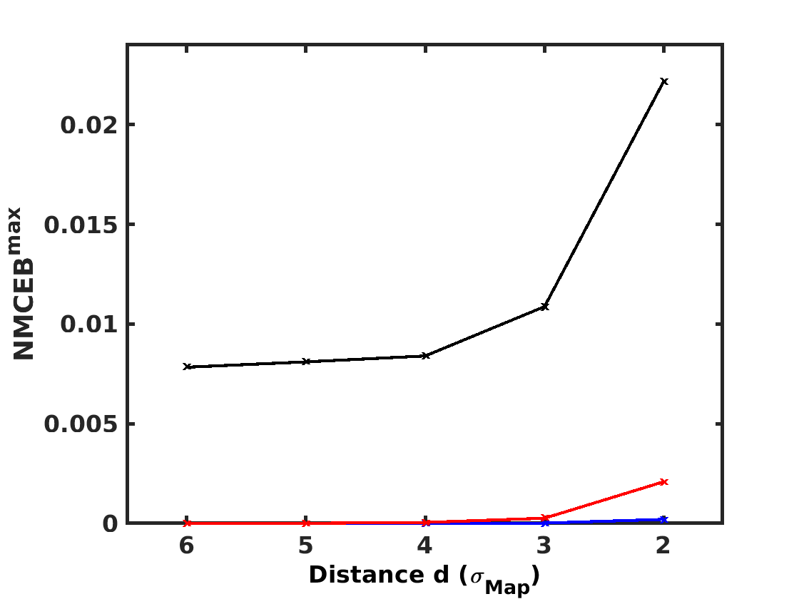
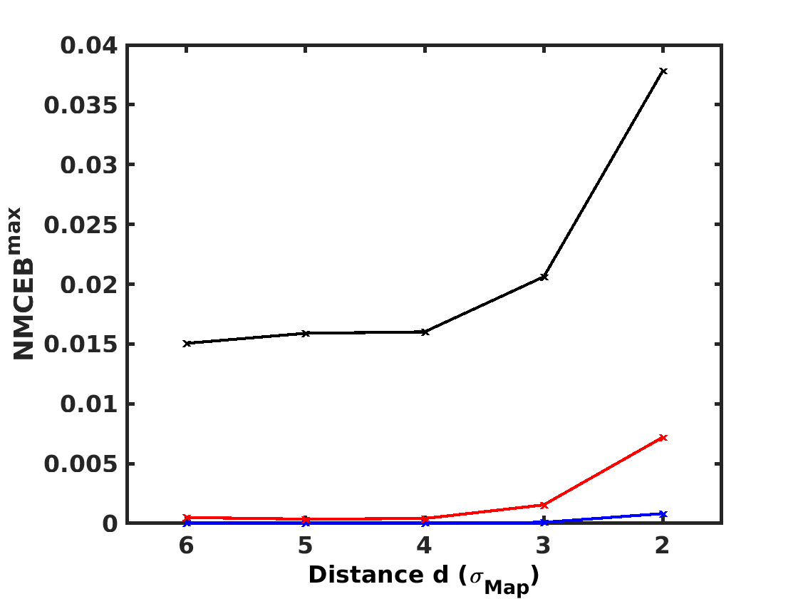
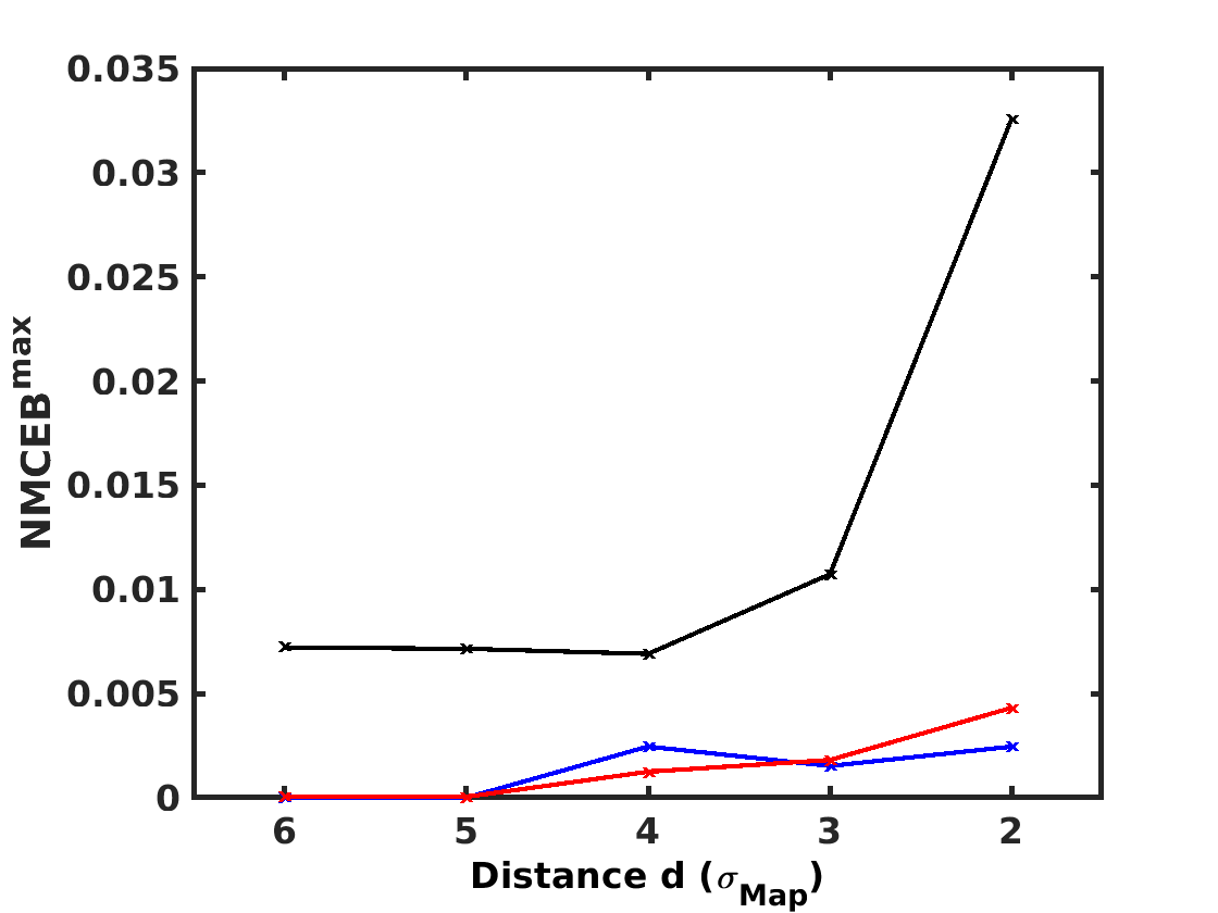
2 sources	4 sources	6 sources

Figure 21: Spread (NMCEB) of the solutions of MASS-NMF-Map obtained on the 45 synthetic cubes with 100 realizations of noise.

B.8 Results for very low signal-to-noise ratios

Finally, we performed additional tests for the two methods which appeared to be the most attractive ones in Section 5.3.3, namely MASS-NMF-Map and SC-NMF-Map. These tests aim at further analyzing the behavior of these preferred methods for very low SNRs, that is five, three, and one dB. The results thus obtained are shown in Fig. 22 and 23. This shows that SC-NMF-Map here yields significantly better performance than MASS-NMF-Map, as opposed to the results obtained in Section 5.3.3 for significantly higher SNRs. This difference is reasonable and coherent with the comments that we provided in Section B.5: although SC-NMF-Map is constraining in terms of sparsity requirements, it has the advantage of averaging the data over an analysis zone (instead of using a single point in the basic version of MASS-based methods), which reduces its sensitivity to noise. For very noisy data, such as those considered here, this feature is of utmost importance, so that SC-NMF-Map yields better performance than MASS-NMF-Map.

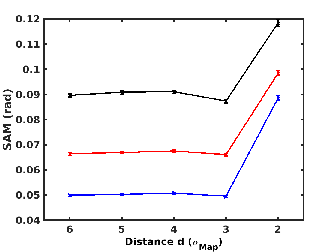
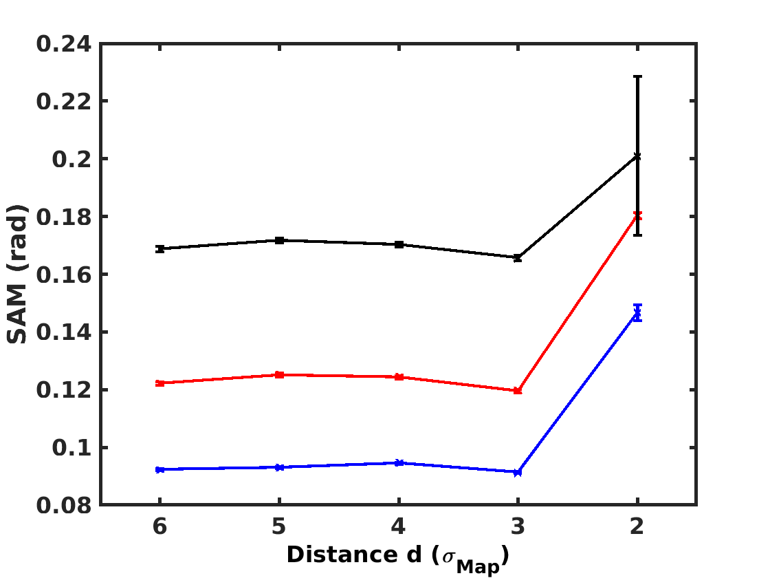
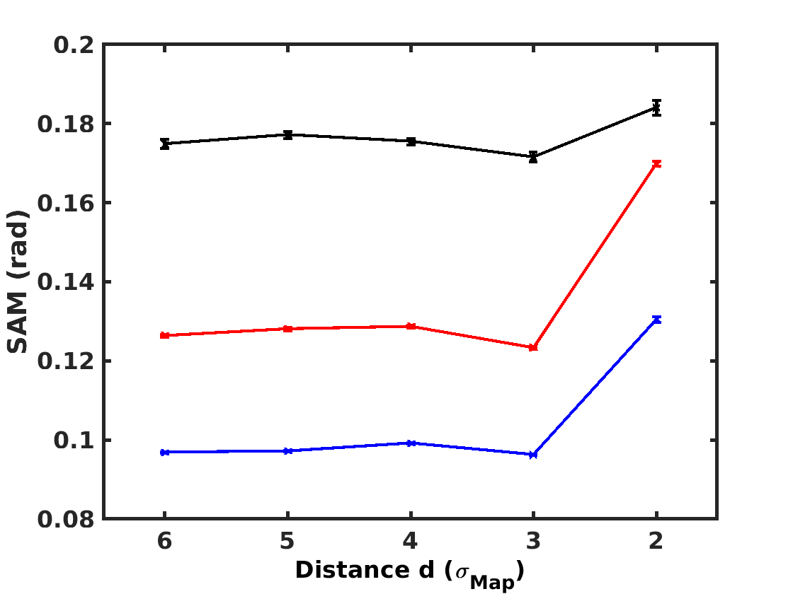
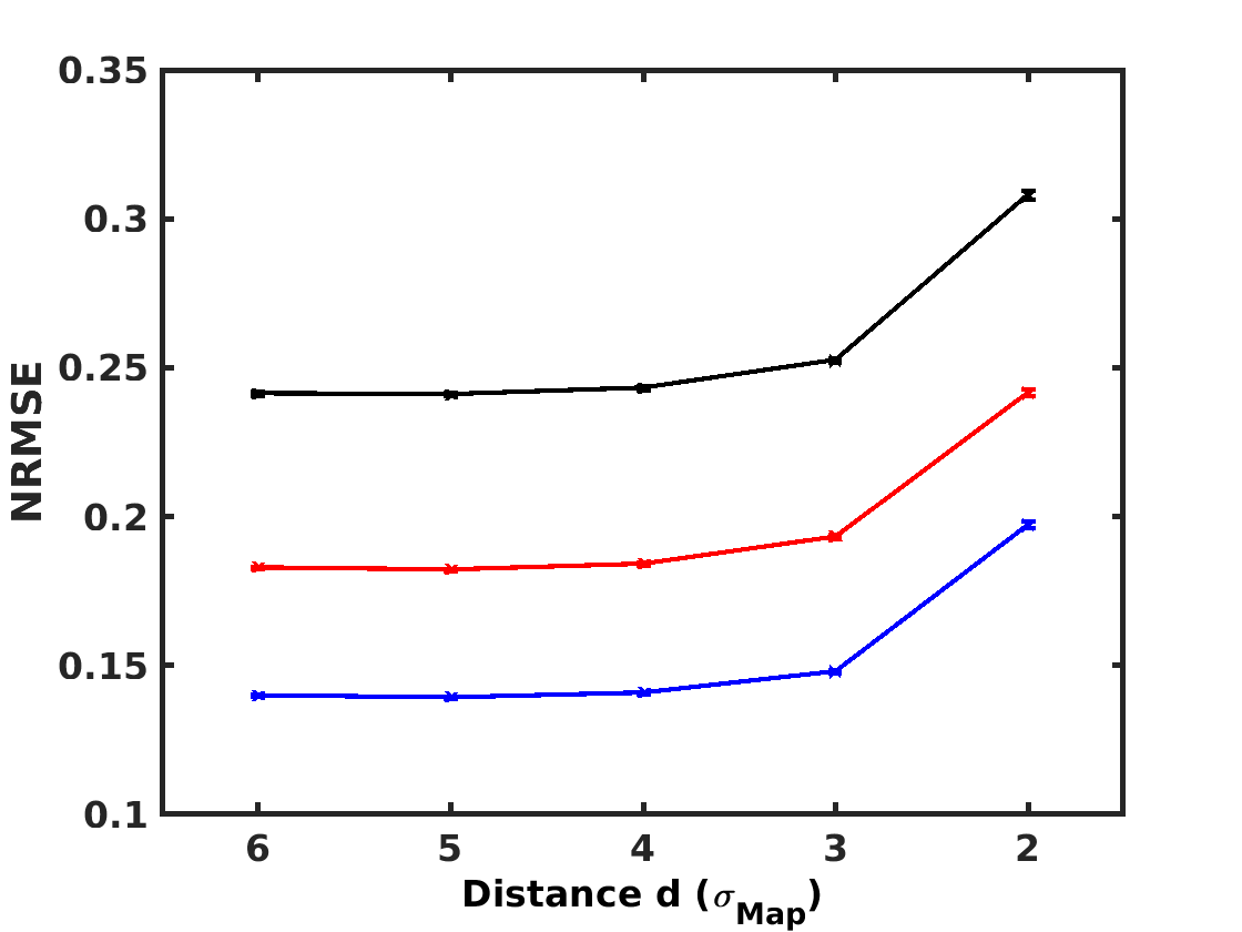
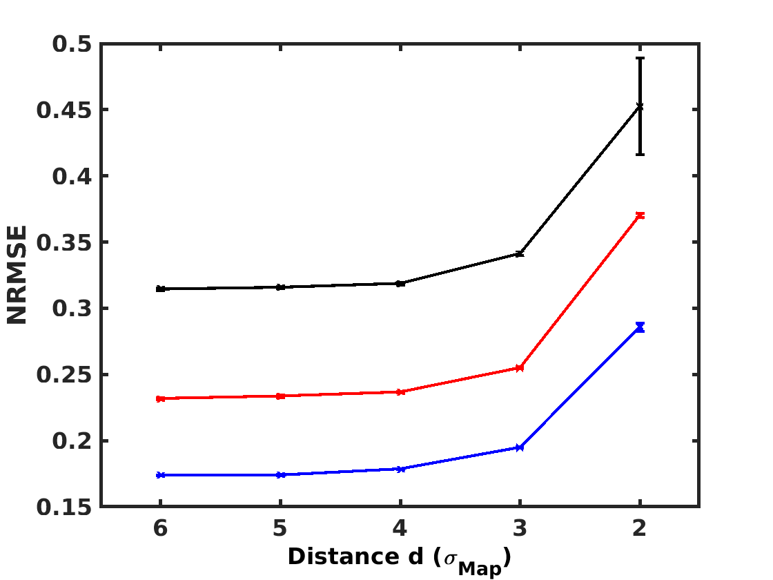
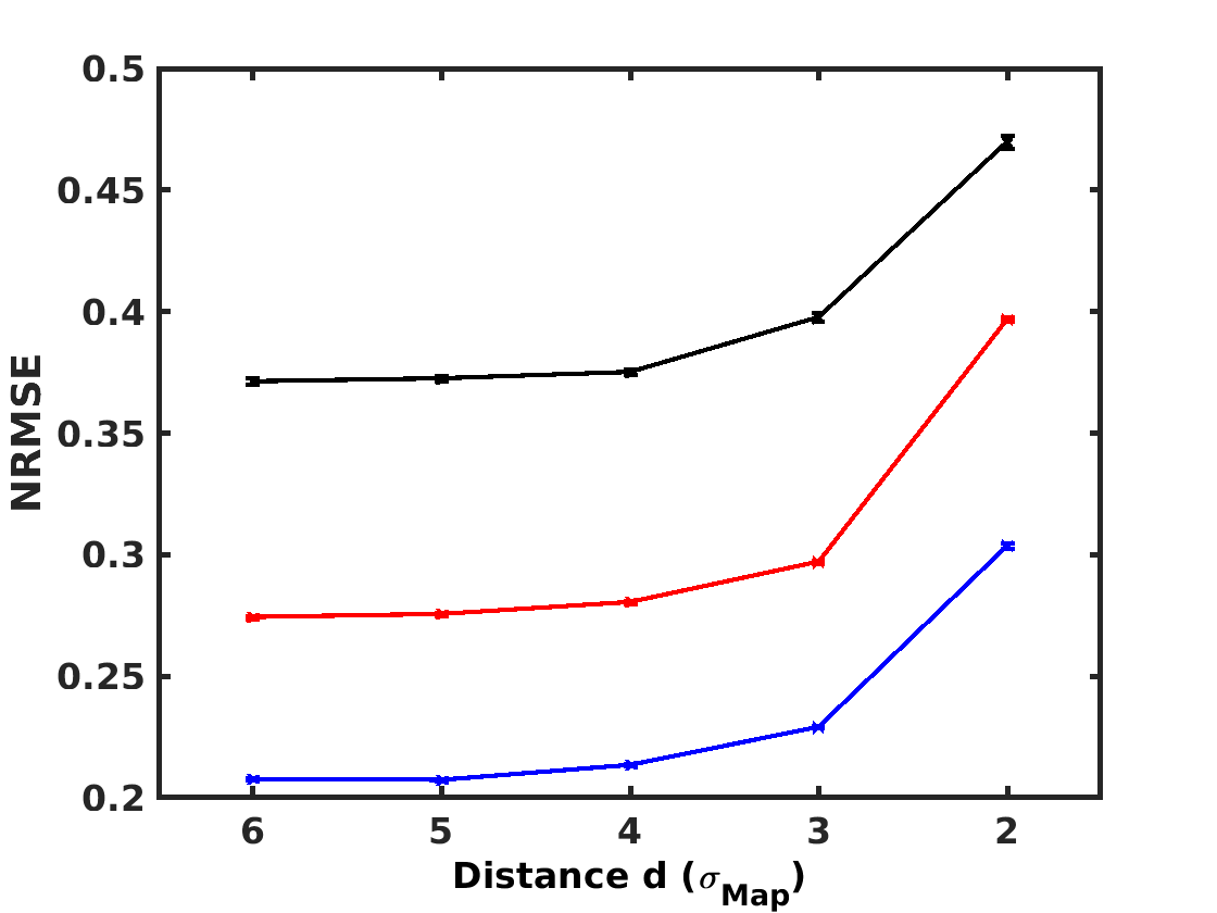
2 sources	4 sources	6 sources

Figure 22: Performances achieved by SC-NMF-Map on the 45 synthetic cubes for 100 realizations of noise with an SNR of 5 dB (in blue), 3 dB (in red), and 1 dB (in black). The error bars give the standard deviation over the 100 realizations of noise.

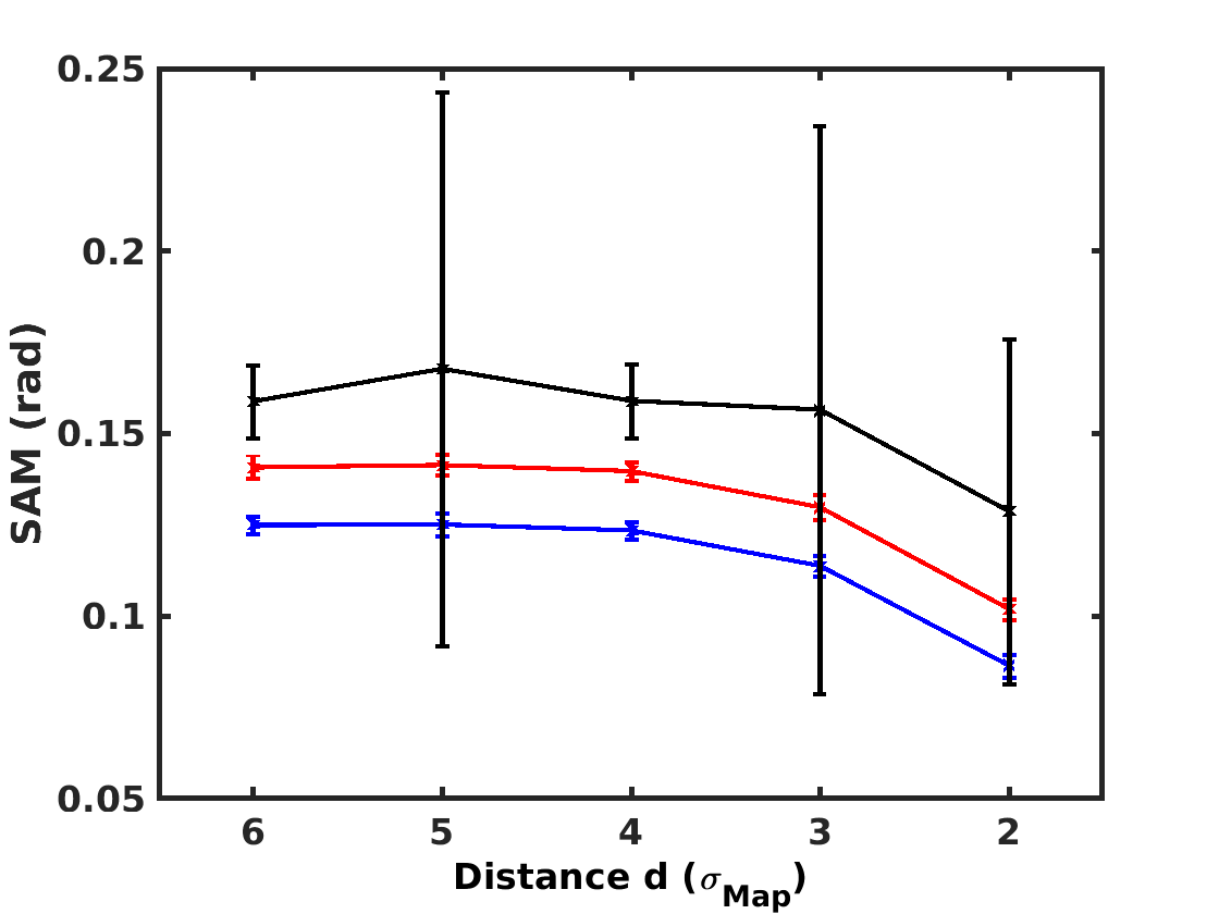
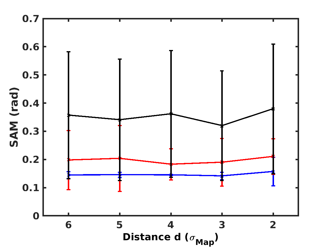
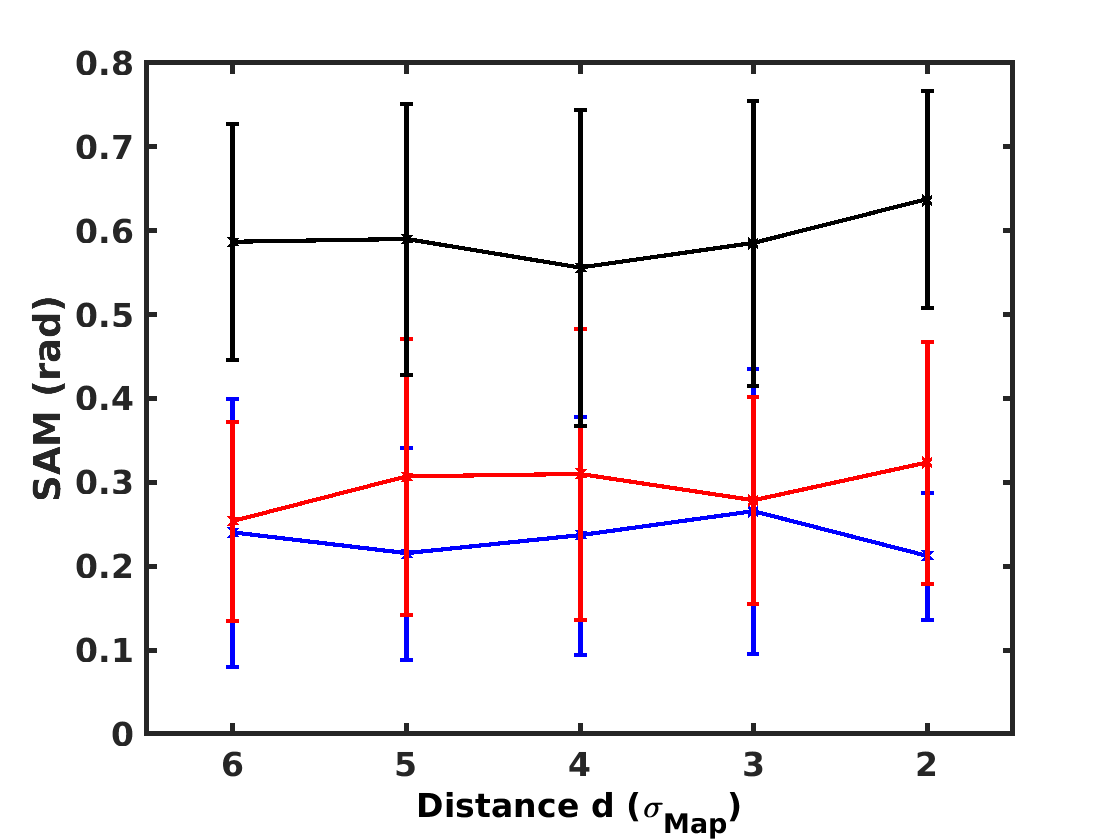
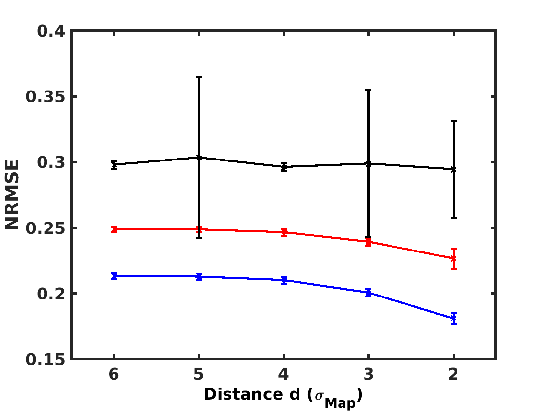
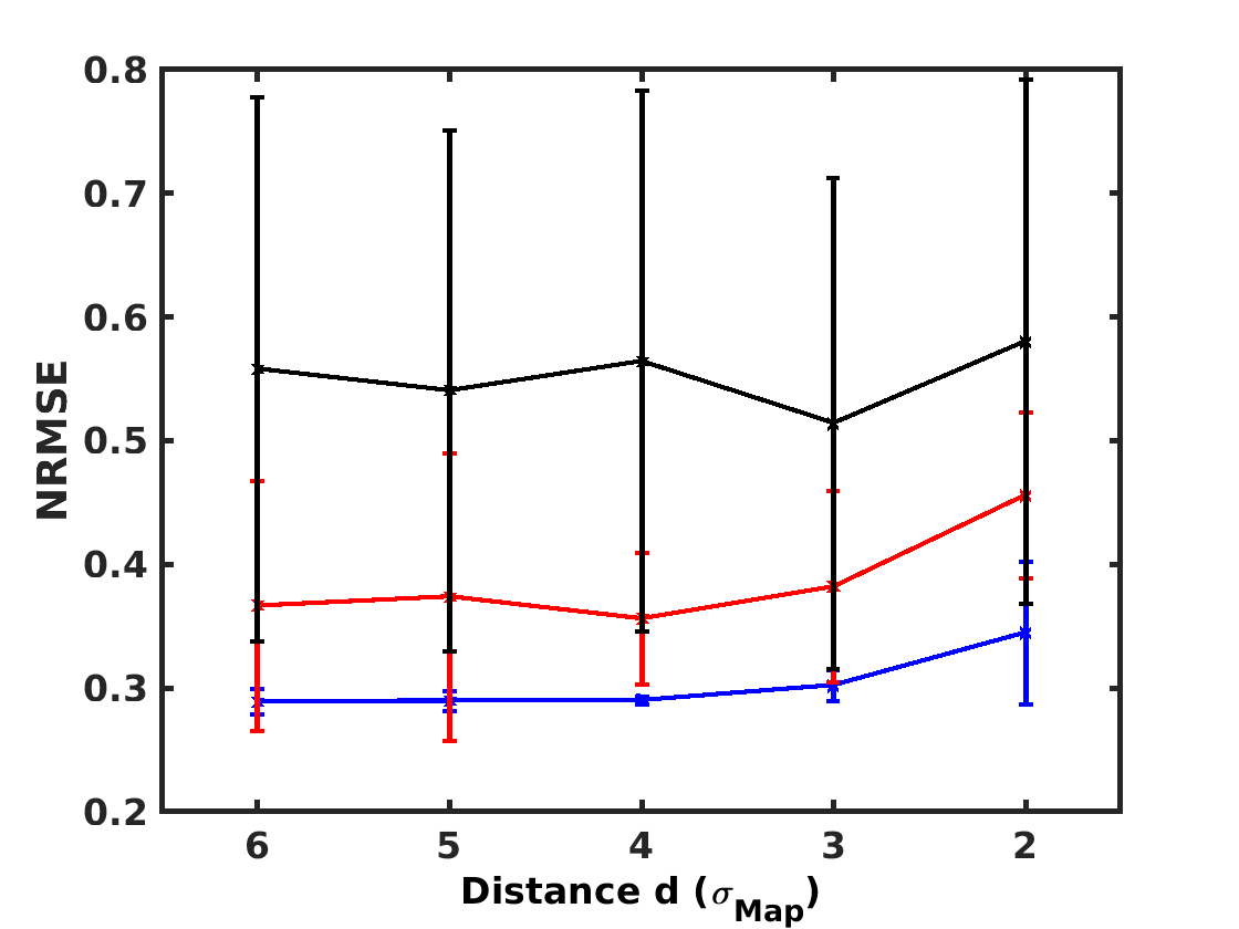
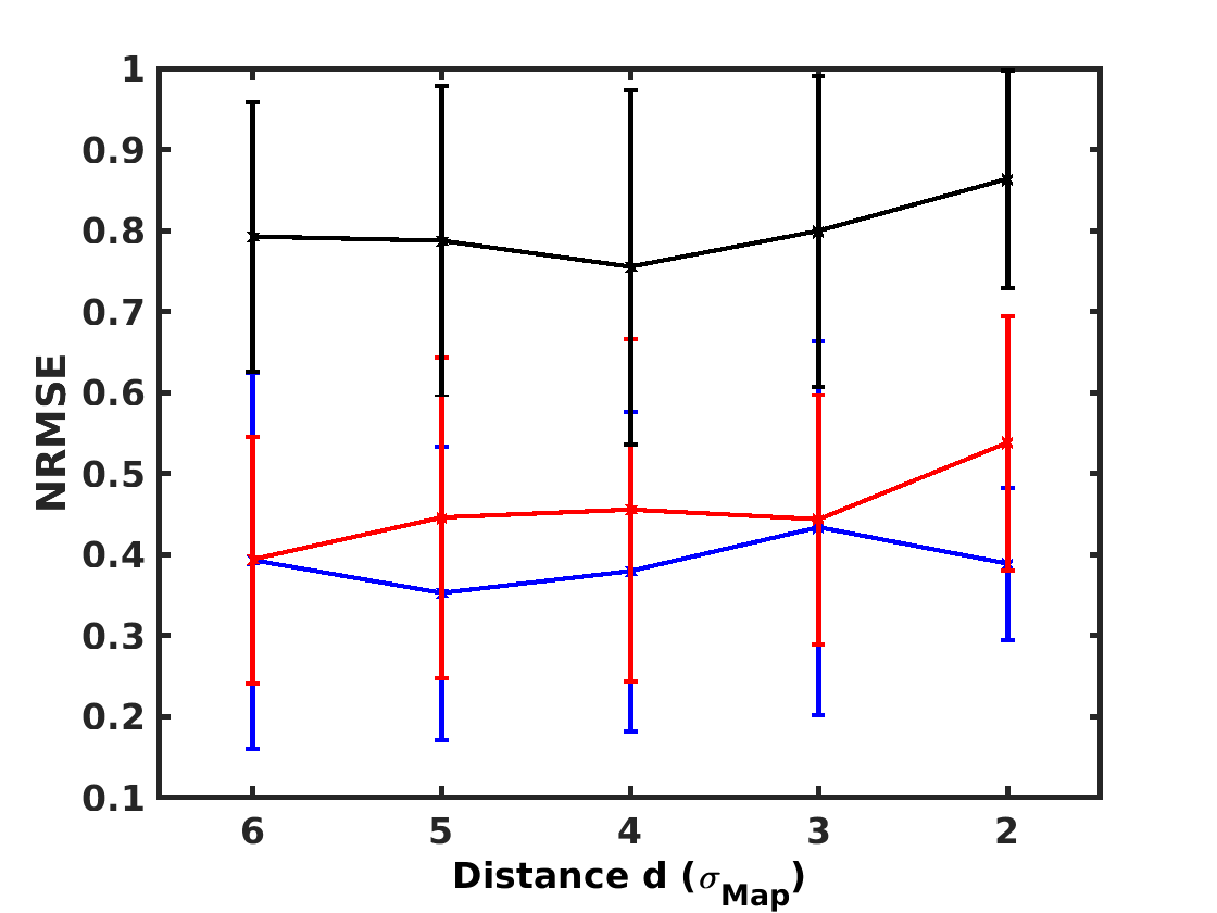
2 sources	4 sources	6 sources

Figure 23: Performances achieved by MASS-NMF-Map on the 45 synthetic cubes for 100 realizations of noise with an SNR of 5 dB (in blue), 3 dB (in red), and 1 dB (in black). The error bars give the standard deviation over the 100 realizations of noise.

B.9 Results for asymmetric scenes

Here we test the effect of breaking the symmetry of the spatial scene presented in Fig 4. We do these by two means, 1) we decrease the size of some sources, 2) we displace one of the sources outside the square grid considered so far. These two cases are illustrated in Fig. 24. We have considered other variations as well (e.g. smaller or larger displacement). Overall, the analysis of the results shows that the methods provide results with similar performances as for the standard cases described in the core of the paper. Hence, the symmetry of the scene does not appear to be critical, as long as the important hypotheses required by the methods (positivity and sparsity) are verified.

Figure 24: Two cases of symmetry breaking for the maps : reduction of the size of two spatial sources (left) and displacement of one source (right).

References

- Bally et al. (1987) Bally, J., Lanber, W. D., Stark, A. A., & Wilson, R. W. 1987, ApJ, 312, L45
- Berné et al. (2012) Berné, O., Joblin, C., Deville, Y., et al. 2012, in SF2A-2012: Proceedings of the Annual meeting of the French Society of Astronomy and Astrophysics, ed. S. Boissier, P. de Laverny, N. Nardetto, R. Samadi, D. Valls-Gabaud, & H. Wozniak, 507–512
- Berné et al. (2007) Berné, O., Joblin, C., Deville, Y., et al. 2007, A&A, 469, 575
- Boulais et al. (2015) Boulais, A., Deville, Y., & Berné, O. 2015, IEEE International Workshop ECMSM
- Cardoso (1998) Cardoso, J.-F. 1998, Proceedings of the IEEE, 86, 2009
- Cesarsky et al. (1996) Cesarsky, D., Lequeux, J., Abergel, A., et al. 1996, A&A, 315, L305
- Cichocki et al. (2009) Cichocki, A., Zdunek, R., Phan, A., & Amari, S.-I. 2009, Nonnegative matrix and tensor factorizations: Applications to exploratory multi-way data analysis and blind source separation (John Wiley and Sons)
- Deville (2014) Deville, Y. 2014, Blind Source Separation: Advances in Theory, Algorithms and Applications. Chapter 6, Sparse component analysis: a general framework for linear and nonlinear blind source separation and mixture identification (pp. 151-196) (Springer)
- Deville & Puigt (2007) Deville, Y. & Puigt, M. 2007, Signal Processing, 87, 374
- Deville et al. (2014) Deville, Y., Revel, C., Briottet, X., & Achard, V. 2014, IEEE Whispers
- Donoho & Stodden (2003) Donoho, D. & Stodden, V. 2003, in (MIT Press), 2004
- Falgarone et al. (2009) Falgarone, E., Pety, J., & Hily-Blant, P. 2009, A&A, 507, 355
- Foschino et al. (2019) Foschino, S., Berné, O., & Joblin, C. 2019, A&A
- Goicoechea et al. (2016) Goicoechea, J. R., Pety, J., Cuadrado, S., et al. 2016, Nature, 537, 207
- Gratier et al. (2017) Gratier, P., Bron, E., Gerin, M., et al. 2017, A&A, 599, A100
- Gribonval & Lesage (2006) Gribonval, R. & Lesage, S. 2006, in ESANN’06 proceedings - 14th European Symposium on Artificial Neural Networks (Bruges, Belgium: d-side publi.), 323–330
- Guilloteau et al. (2019) Guilloteau, C., Oberlin, T., Berné, O., & Dobigeon, N. 2019, A&A
- Habart et al. (2010) Habart, E., Dartois, E., Abergel, A., et al. 2010, A&A, 518, L116+
- Hyvärinen et al. (2001) Hyvärinen, A., Karhunen, J., & Oja, E. 2001, Independent component analysis, Vol. 26 (Wiley-interscience)
- Joblin et al. (2010) Joblin, C., Pilleri, P., Montillaud, J., et al. 2010, A&A, 521, L25+
- Juvela et al. (1996) Juvela, M., Lehtinen, K., & Paatero, P. 1996, MNRAS, 280, 616
- Kristensen et al. (2011) Kristensen, L. E., van Dishoeck, E. F., Tafalla, M., et al. 2011, A&A, 531, L1
- Langville et al. (2006) Langville, A., Meyer, C., & Albright, R. 2006
- Lawson (1974) Lawson, C. 1974, Solving Least Squares Problems (Classics)
- Lee & Seung (1999) Lee, D. D. & Seung, H. S. 1999, Nature, 401, 788
- Lee & Seung (2001) Lee, D. D. & Seung, H. S. 2001, in In NIPS (MIT Press), 556–562
- Luo & Zhang (2000) Luo, J. & Zhang, Z. 2000, in Signal Processing Proceedings, Vol. 1, 223–225
- Meganem et al. (2010) Meganem, I., Deville, Y., & Puigt, M. 2010, Acoustics Speech and Signal Processing (ICASSP), 2010 IEEE International Conference on, 1334
- Miao & Qi (2007) Miao, L. & Qi, H. 2007, IEEE Transactions on Geoscience and Remote Sensing, 45, 765
- Miesch & Bally (1994) Miesch, M. S. & Bally, J. 1994, ApJ, 429, 645
- Neufeld et al. (2007) Neufeld, D. A., Hollenbach, D. J., Kaufman, M. J., et al. 2007, ApJ, 664, 890
- Paatero & Tapper (1994) Paatero, P. & Tapper, U. 1994, Environmetrics, 5, 111
- Pabst et al. (2017) Pabst, C. H. M., Goicoechea, J. R., Teyssier, D., et al. 2017, A&A, 606, A29
- Pilleri et al. (2012) Pilleri, P., Montillaud, J., Berné, O., & Joblin, C. 2012, A&A, 542, A69
- Silverman (1998) Silverman, B. 1998, Density Estimation for Statistics and Data Analysis (Chapman and Hall/CRC)
- Theodoridis & Koutroumbas (2009) Theodoridis, S. & Koutroumbas, K. 2009, Pattern Recognition (Academic Press)
- Van Kempen et al. (2010) Van Kempen, T. A., Kristensen, L. E., Herczeg, G. J., et al. 2010, A&A, 518, L121+
- Weilbacher et al. (2015) Weilbacher, P. M., Monreal-Ibero, A., Kollatschny, W., et al. 2015, A&A, 582, A114
- Werner et al. (2004) Werner, M. W., Uchida, K. I., Sellgren, K., et al. 2004, ApJS, 154, 309