SOCAIRE: Forecasting and Monitoring Urban Air Quality in Madrid

Abstract

Air quality has become one of the main issues in public health and urban planning management, due to the proven adverse effects of high pollutant concentrations. Considering the mitigation measures that cities all over the world are taking in order to face frequent low air quality episodes, the capability of foreseeing future pollutant concentrations is of great importance. Through this paper, we present SOCAIRE, an operational tool based on a Bayesian and spatiotemporal ensemble of neural and statistical nested models. SOCAIRE integrates endogenous and exogenous information in order to predict and monitor future distributions of the concentration for several pollutants in the city of Madrid. It focuses on modeling each and every available component which might play a role in air quality: past concentrations of pollutants, human activity, numerical pollution estimation, and numerical weather predictions. This tool is currently in operation in Madrid, producing daily air quality predictions for the next 48 hours and anticipating the probability of the activation of the measures included in the city’s official air quality NO₂ protocols through probabilistic inferences about compound events.

Keywords Air Quality  $\cdot$ Spatio-temporal Series  $\cdot$ Statistical Modeling  $\cdot$ Neural Networks

1 Introduction

During the last decades, an increasing number of studies point out that degraded air quality is a major problem in cities around the world [24, 14]. While there is general consensus that it causes health problems [18, 31], how dangerous it can be is still a matter of debate [33]. Even in the best case scenario, this seemingly endemic issue affecting the life in big cities is already considered one of the main causes of both direct and indirect mortality [2].

Of all the tools and systems that help fight pollution, the prediction of future pollutant concentrations or levels is of principal importance for air quality management and control [3]. Air quality forecasting systems allow for sending out warnings of upcoming high pollution episodes to the population in the short-term, so that appropriate measures can be taken to minimize as far as possible the damage caused by these episodes. As an example, the city of Madrid, in order to comply with European regulations [36], devised an air quality protocol which includes restrictions to the use of polluting vehicles when the concentrations of NO₂ reach certain thresholds. Consequently, foreseeing the activation of such restrictions is critical both for the decision makers (which need to announce them in advance) and for the vehicle owners (which need to plan their transport alternatives).

The use of data-driven approaches to predict and control air quality is not new. Following the discussion started by Breiman [6], when approaching a modeling problem two families of methodologies (or “cultures”, in Breiman terms) coexist: the data modeling culture, based on the search for a stochastic data model (for example, time difference equations, in the case of air quality) that capture the inner behavior of the intervening physical processes, and the algorithmic modeling culture, based on the use of algorithms to directly learn the model from data. Given that pollutant concentrations can be seen as time series, the stochastic data modeling usually deals with using ARMA based methods [20, 13]. However, this kind of models have trouble handling high non-linearities and high dimensional environments. To solve this problem, and thanks to the big amount of data that is gathered nowadays, machine learning models have been applied to environmental modeling with some success [12, 27]. In this work, however, we advocate for a hybrid “culture”, in which stochastic data models are combined with algorithmic ones in a way which permits harvesting the benefits of both approaches while reducing their disadvantages, as we will show.

Due to the increase in the available computing power and the advances in the field of neural network-based models, it is nowadays common to find real applications in which algorithmic modeling is put into practice to predict air quality. For example, in [28] a system is deployed in which pollution levels based on a threshold are used to study transitions among states, which makes possible to estimate high pollution episodes in the long term. In [35], authors have combined the TAPM and CCAM atmospheric models to form a customizable, local-scale meteorological and air pollution forecasting system, showing that using macroscopic models in the local scale can provide positive points in the prediction. [22] is an example of an ensemble model with a neural network and an ARIMA, in a similar vein to what will be our proposal, applied successfully to a real urban environment in the city of London.

For this kind of real applications, it is useful to produce, instead of a forecast of the expected value of the magnitude under study, an estimation of the full future distribution, which in turn allows for decision making based on the probability of the surpassing of certain thresholds. This idea, which will ultimately be the main goal of the system described below, is common in other fields and was introduced to air pollution forecasting by [1].

The integration of meteorological information and human activities have been addressed by multiple studies. Some relevant variables, as temperature, precipitation, or wind speed have shown to be good indicators of pollution levels [17, 30, 19]. Also, the physical-chemical mechanisms governing the relationship between these and air quality has been studied. In [37], interpretability techniques for deep learning are used to gain insight into feature importance in a highly similar environment and methodology to ours, concluding that weather variables, in general, have a high impact when using machine learning methods for predicting pollution.

However, while these issues have been widely studied from the univariate time series perspective, the observed spatial interactions between nearby observation stations might be of importance too as air quality at different stations might be implicitly related. Spatial-based approaches usually imply assuming or learning these interdependencies based for example on closeness, but, as it has been shown [25], this is not necessarily the most natural and optimal way to go.

In this paper, we introduce SOCAIRE, the new official air quality monitoring system for the city of Madrid. This tool, in operational use nowadays, makes use of both external and internal variables related to air quality in order to forecast pollutant concentrations. It is a complex modular mathematical system composed of an ensemble of data manipulation techniques and models that let us exploit different knowledge in each module: from data cleaning and imputation, through handling spatial and meteorological non-linear features, to integrating human behavior and its patterns. By correctly treating all this information, it is possible to avoid redundancies and to achieve very high performance. As one of the biggest and most populated cities in Europe, Madrid is a perfect setting for developing and testing these kind of systems.

The rest of the paper is organized as follows: in Section 2 the problem is stated and Madrid’s air quality protocol for NO₂ is described, while Section 3 presents an analysis and explanation of the different data sources and the data wrangling process. Section 4 presents the proposed approach for air quality forecasting. Then, in Section 5 we introduce the Bayesian probabilistic framework that let us accommodate SOCAIRE to the NO₂ protocol. Section 6 shows the evaluation of the proposed architecture after appropriate experimentation and its comparison with other methodologies. Finally, in Section 7 we point out future research directions and conclusions.

2 Problem statement

2.1 Study area and general information

(a) Location of all measurement stations.

(b) Zones definition for NO₂ protocol.

Figure 1: Location of pollutant measurement stations and definition of the 5 different areas in which the NO₂ protocol divides the city.

Table 1: Locations and availability of pollution variables for each station. A ✓reflects the presence of data in the corresponding location and for the corresponding pollutant.

Station	Code	Long.	Lat.	NO2	O3	PM10	PM2.5
Pza. de España	4	-3.712	40.423	✓	-	-	-
Escuelas Aguirre	8	-3.682	40.421	✓	✓	✓	✓
Avda. Ramón y Cajal	11	-3.677	40.451	✓	-	-	-
Arturo Soria	16	-3.639	40.440	✓	✓	-	-
Villaverde	17	-3.713	40.347	✓	✓	-	-
Farolillo	18	-3.731	40.395	✓	✓	✓	-
Casa de Campo	24	-3.747	40.419	✓	✓	✓	✓
Barajas Pueblo	27	-3.580	40.477	✓	✓	-	-
Pza. del Carmen	35	-3.703	40.419	✓	✓	-	-
Moratalaz	36	-3.645	40.408	✓	-	✓	-
Cuatro Caminos	38	-3.707	40.446	✓	-	✓	✓
Barrio del Pilar	39	-3.711	40.478	✓	✓	-	-
Vallecas	40	-3.652	40.388	✓	-	✓	-
Mendez Alvaro	47	-3.687	40.398	✓	-	✓	✓
Castellana	48	-3.690	40.439	✓	-	✓	✓
Parque del Retiro	49	-3.683	40.414	✓	✓	-	-
Plaza Castilla	50	-3.689	40.466	✓	-	✓	✓
Ensanche de Vallecas	54	-3.612	40.373	✓	✓	-	-
Urb. Embajada	55	-3.581	40.462	✓	-	✓	-
Pza. Elíptica	56	-3.719	40.385	✓	✓	✓	✓
Sanchinarro	57	-3.661	40.494	✓	-	✓	-
El Pardo	58	-3.775	40.518	✓	✓	-	-
Juan Carlos I	59	-3.616	40.461	✓	✓	-	-
Tres Olivos	60	-3.689	40.501	✓	✓	✓	-

Through this work, we look for a system which is able to predict up to 48 hours of four of the main existing pollutants: Nitrogen dioxide (NO₂), ozone (O₃), and particulate matter PM10 and PM2.5, where 10 and 2.5 denote the maximum diameters (in micrometers) of the particles. This estimation needs to be done in the 24 stations that compose the pollution measurement network, each one with different pollutants. Since one of the main objectives of the system is to anticipate the activation of mobility restrictions in face of high pollution episodes, we forecast the main quantiles of the distribution, so it is easier to make decisions based on pollution level probabilities. Thanks to its Bayesian estimation of compound events, SOCAIRE becomes an ideal tool to foresee the scenarios of Madrid’s NO₂ protocol, which will be explained later in this section.

SOCAIRE operates daily on a 48-hours basis: it produces forecasts from 10:00 of the present day to 09:00 two days later. In the spatial dimension, the measurement stations of the city council are used as reference points. Specifically, there are 24 stations distributed throughout the city with sensors capable of recording different pollutants. Fig. 1(a) shows graphically the location of all the stations. At the same time, the city considers 5 different areas in the city that are related to the activation of the NO₂ protocol. These areas are shown in Fig. 1(b). Table 1 shows the correspondence between the different stations and their code, their location, and the pollutants measured at each one.

2.2 The NO₂ protocol of the city of Madrid

In 2018, the city council of Madrid approved an “Action Protocol for NO₂ Pollution Episodes” [32] (from this point, referred to as “the NO₂ protocol”) which defines a set of increasing alert levels, thus classifying the situations of high concentrations of NO₂ as follows:

1. PREWARNING: when any two stations in the same area simultaneously exceed 180 $\mathrm{\mu gm^{-3}}$ for two consecutive hours, or any three stations in the surveillance network simultaneously exceed the same level for three consecutive hours.

2. WARNING: when any two stations in the same area exceed 200 $\mathrm{\mu gm^{-3}}$ during two consecutive hours, or any three stations in the surveillance network exceed the same level simultaneously during three consecutive hours.

3. ALERT: when in any three stations of the same zone (or two if it is zone 4) is exceeded simultaneously, 400 $\mathrm{\mu gm^{-3}}$ during three consecutive hours.

Depending on the level and the meteorological prospect, a set of increasingly restrictive mobility limitations will be imposed city-wide by the council with the aim of mitigating and reducing the negative effects of contamination on the health and integrity of the population. Thus, the main objective is to know when and how the conditions leading to the different alert levels will be met, in order to enable the anticipation of the measures.

2.3 Framework overview

Figure 2: The mathematical components of SOCAIRE.

Fig. 2 presents a summary of SOCAIRE’s mathematical structure. Created to forecast and monitor pollution levels, its operation is based on the compilation of several data sources which will be described in Section 3. After a proper analysis and cleaning process, the complete database will be used through an ensemble model composed of a cascade of nested models, each one in charge of modeling different processes that alter air quality dynamics (Section 4). Finally, and thanks to the probabilistic nature of the predictions, the system is able to estimate probabilities from compound events using a Bayesian approach explained in Section 5 that is adapted to the aforementioned NO₂ protocol.

3 Data analysis and wrangling

As stated above, in order to aim for the highest performance, SOCAIRE makes use of all the available information related to the problem. Thus, before introducing the actual modeling, it is important to present and analyze the set of available data sources. Concretely, as anticipated, SOCAIRE uses the data of the concentrations of the different pollutants in the different stations in Madrid as dependent variables (output) and, as independent variables (inputs), past pollutant concentrations, numerical pollution predictions coming from the European CAMS model [7], numerical weather predictions served by AEMet [26], and anthropogenic information encoding different events such as holidays and school calendar. The following subsections will detail the origin, peculiarities, and processing of these data.

3.1 Pollutants

Figure 3: Hourly, daily, and monthly temporal distribution of the four target pollutants.

Figure 4: Distribution of the series by pollutant and station.

The temporal behavior of each pollutant series is shown in Fig. 3. The daily cycle of all pollutants is dominated in one way or another by the peak hours of road traffic. Except for ozone, the other three pollutants to be analyzed have their daily peaks after peak traffic hours. The NO₂ has the most intense traffic-sensitive cycle, followed by the 10 and 2.5 microparticles, which show a delay of about an hour with respect to the NO₂. O₃ presents a daily cycle that is practically inverted with respect to the rest.

Everything said for the daily cycle applies to the weekly cycle, with weekend being days with lower levels of traffic. It can be assumed that holidays and long weekends will behave as public holidays, so the forecast model would have to take this into account. As expected, the daily cycle is not independent of the weekly one, but each day of the week has its own cycle, especially different on weekends from working days.

In the annual cycles, a greater variety of behaviors can be observed. All pollutants, especially ozone, rebound in summer except NO₂ which has the opposite behavior in this case.

Respect to the spatial dimension, Fig. 4 represents the empirical distributions for each pollutant. It can be seen that all stations report a similar behavior, without clear relation patterns between closeness and distribution. This fact will be of interest later when taking into account these spatial relationships in the modeling process.

As the distributions show a clear asymmetry, logarithmic transformations are used. Pollutant data is publicly available at the Open data portal of Madrid [8].

3.2 Numerical weather predictions (NWP)

As mentioned in Section 1, meteorology has shown to be especially important for air quality. Hence, having weather forecasts for the period in which the air quality forecasting is being made is expected to positively impact the precision of the forecasts. In this work, we use NWP from the Integrated Forecasting System (IFS) of the ECMFW [4], for the following set of variables:

• Boundary layer height (in meters): This parameter is the depth of air next to the Earth’s surface which is most affected by the resistance to the transfer of momentum, heat or moisture across the surface. The boundary layer height can be as low as a few tens of meters, such as in cooling air at night, or as high as several kilometers over the desert in the middle of a hot sunny day. When the boundary layer height is low, higher concentrations of pollutants (emitted from the Earth’s surface) are found.

• Surface pressure (in Pa): This parameter is the pressure (force per unit area) of the atmosphere on the surface of land, sea, and in-land water. It is a measure of the weight of all the air in a column vertically above the area of the Earth’s surface represented at a fixed point. Air pollution is especially prominent where high pressure dominates. Subsiding motions within an anticyclone suppress air trying to rise off the surface. Adiabatic warming of subsiding air creates a subsidence inversion which acts as a cap to upwardly moving air. Pollution problems dissipate when a low pressure system replaces a retreating anticyclone.

• Temperature (in K): This parameter is the temperature of air at 2 m above the surface of land, sea, or in-land waters. Generally, higher temperatures and hotwaves are directly related to episodes of higher pollution levels.

• Precipitation (in mm): This parameter is the accumulated liquid and frozen water, including rain and snow, that falls to the Earth’s surface. It is the sum of large-scale precipitation (that precipitation which is generated by large-scale weather patterns, such as troughs and cold fronts) and convective precipitation (generated by convection which occurs when air at lower levels in the atmosphere is warmer and less dense than the air above, so it rises). Precipitation parameters do not include fog, dew, or the precipitation that evaporates in the atmosphere before it lands at the surface of the Earth. Air pollution is typically negatively correlated to the quantity of rainfall, existing a so called washing effect of precipitation.

• U wind component (in $\mathrm{ms^{-1}}$): This parameter is the eastward component of the 10m wind. It is the horizontal speed of air moving towards the east, at a height of ten meters above the surface of the Earth. Pollutants tend to pile up in calm conditions, when wind speeds are not more than about 3 $\mathrm{ms^{-1}}$. Speeds of 4 $\mathrm{ms^{-1}}$ or more favour dispersal of pollutants, which, literally, clears the air.

• V wind component (in $\mathrm{ms^{-1}}$): This parameter is the northward component of the 10 m wind. It is the vertical speed of air moving towards the north, at a height of ten meters above the surface of the Earth. Again, wind is highly related to pollution dissemination.

NWP are interpolated to the location of each station of the air quality monitoring network. As pointed out previously, these forecasts are provided by AEmet in an hourly basis.

3.3 Numerical pollution predictions (NPP)

CAMS (Copernicus Atmosphere Monitoring Service) [7] provides a four day-horizon hourly pollution forecast which covers all Europe on a synoptic scale. The model takes into account global and regional numerical weather predictions from the ECMWF [23], as well as other types of forecasts about the production of certain chemicals of natural and human origin from models such as C-IFS Forecasts or CAMS 81.

All these models always refer to a geodesic grid of between 10 and 20 km on each side, so it is not very sensible to use them to directly forecast the concentrations with the resolution required inside a city, which might well be below one kilometer.

3.4 Anthropogenic features

As we saw in Figure 3, depending on the human activity the temporal patterns of the series are different. Similar to weekends and months, public holidays and other designated days, as well as the school calendar, have a significant influence on road traffic, giving rise to a very different daily cycle. In special dates, we usually find a lower intensity in the center but a punctual growth in other places, particularly on the main access roads to the city related to holiday departures and returns.

Also, each type of calendar effect has different effects on each hour of the day. In addition, some of them can fall on Saturday or even on Sunday, in the case of Christmas Eve and New Year’s Eve, and it is clear that the effect cannot be the same as when it falls during the week, so all these issues must be taken into consideration.

In our particular case, we will take into account the following aspects:

• Public holidays: Public holidays, long weekends, and special days, such as Christmas Eve and New Year’s Eve, are characterized by significantly less road traffic than a normal working day (apart from other departure and return operations that may occur on some of these days and which will be taken into account later).

  It has been observed that public holidays have different effects, both in terms of level and intraday evolution, depending on their location within the year, probably due to climate reasons, hours of light, and living patterns.

• Holiday departures and returns: Extraordinary periods such as bank holidays, long weekends, or even weekends cause a temporary exodus of citizens with large accumulations of vehicles in the so-called departure and return operations.

  Departure operations can take place during the evening of the eve of the first non-working day or during the morning of that day, while return operations occur mostly during the evening of the last holiday, sometimes reaching the early morning of the next working day.

  As with other variables, the effect varies with the hours within a relatively soft form.

• School Calendar: in Spain, school calendar and schedule is highly related to usual hourly, weekly, and monthly patterns and so, it can model with high precision the daily living. The school day can be complete or normal, average (pre- and post-holidays) or non-existent, either in isolation or for summer, winter nor spring holidays. Each type of day other than the normal one is introduced as an effect with a different intraday cycle between 07:00 and 08:00.

By combining all these variables, we ensure that the information relating to human mobility in the city is covered, both for normal situations and for special events. These exogenous variables are defined for each station, as not all parts of the city have the same dynamics.

3.5 Data wrangling

When working with such diverse data sources, is usual to deal with very heterogeneous formats and criteria, which implies that pre-processing and cleaning steps are of utmost importance. Some of the most important ones for this project are listed in this section.

Firstly, some sources use UTC time and others use Madrid’s local time. In addition, the processes that transfer data between different programming environments (R, TOL, and Python) also have to take into account that each of these systems work differently with respect to winter and summer daily savings time changes.

Secondly, both NWP and NPP distribute their forecasts in a different geodesic grid, which in turn does not coincide with the coordinates of the pollution monitoring stations. At first, an attempt of interpolation was made by using the three closest grid points to each station as drivers, but it soon became apparent that this was an excessive complication with very little added value, as the forecasts were highly correlated. Therefore, in the final version, only the nearest reticular point to each station is used.

Thirdly, weather predictions are not always in the most appropriate metric, so it is necessary to create derived variables that serve better as drivers of the models. To begin with, there are variables that change scale throughout history and it is necessary to unify the criterion for obtaining uniform series in time. Then, there are other variables that are interesting to modify conceptually, for example, instead of the east-west and north-south coordinates of wind speed, it is much better to use scalar speed, which is the fundamental factor of diffusion, and direction, which is less important. Finally, it is known that meteorological factors not only have an instantaneous effect, but also a delayed effect that can be exercised up to a few hours later. For this reason, some variables delayed up to 4 hours have been created and integrated with the rest of features.

Finally, since we are dealing with a cascade-like ensemble of models, in which the output of one is the input of another which may require a substantially different structure, each level of modeling requires a series of steps to prepare the data to be as expected in the next phase.

Let us note that the most laborious part of the data pre-processing has been the imputation of missing values. However, given the importance of this part, it has been decided to include imputation of data as part of the modeling strategy and is explained later in section 4.1.

4 Modeling Strategy

The concentration of a given pollutant in the air depends on at least two conceptually distinct groups of factors:

• Emission factors: generally these are of a social order, such as road traffic or heating, which are predictable to some extent, although there are also totally unpredictable events such as fires, and others that could be anticipated to some extent such as strikes or sporting events with a multitudinous following.

• Dispersion factors: basically these are consequences of the weather conditions on which there are quite precise forecasts on the horizon of 2 or 3 days ahead.

Note that a certain factor, such as rain, can work in both directions at the same time: on the one hand it can cause an increase in traffic on a normal working day, which increases pollution, but on the other hand it disperses, especially the particles as they are carried to the ground, which decreases pollution. It is even possible that the effect is different depending on the day and time. Following the example of the rain that normally increases the traffic in a working day, it can on the contrary contract the traffic in an exit operation, when it will discourage people to leave the city.

This causal complexity, added to the high degree of interaction between factors, makes the phenomenon highly unstable and therefore very difficult to predict using any individual methodology. For this reason, an ensemble model composed of a cascade of nested models has been designed, such that the output of each is used in the next to get the most out of each:

• Imputation techniques: Although this task is usually framed as part of the data wrangling process, in this project it involves the development of models of some complexity, due to the fact that the omitted elements are presented with a certain frequency and not always in a sporadic way, but covering periods of time that can even be of several weeks. These techniques are detailed in Section 4.1.

• NNED model: a special flavor of convolutional neural networks called neural net encoder-decoder, which, using as inputs the outputs of the imputation models, allows to jointly forecast the concentrations of a pollutant in all the stations at the same time. It takes into account the NWP and NPP, as well as the recent past of all stations for each input variable, including the previous pollution itself, and is capable of automatically detecting non-linearities and interactions between different features. However, it does not allow for the natural treatment of irregularities in non-cyclical anthropogenic factors related with traffic. It is described in detail in Section 4.2.

• PP-NNLS-ARFIMA-QR model: This is a chain of models by itself developed specifically to deal with anthropogenic factors in a Bayesian way. It will be explained in detail in Section 4.3.

4.1 Imputation techniques

Figure 5: Imputation scheme. All data sources likely to have missing values are part of the process. Through successive refinements, the initial data are processed through different techniques in a way that takes into account the nature and particularity of each source when performing the task. Black-dashed arrows follow processes in which data has not been imputed yet, while blue-solid arrows formalize the idea that this particular set has already been imputed.

In the different data sources, it is relatively frequent to find missing data that can cause problems in the modeling process. For this reason, it is necessary to devise a sensible way to fill in these missing values, replacing them with approximate or expected values by a series of auxiliary models. When there are only very sporadic omissions of short duration, it might be sufficient to apply some kind of approximation by interpolation, but there might be up to consecutive weeks of data omitted in several or all variables from one or more sources at the same time. Thus, in order to develop a robust operational system, able to function even in the presence of missing data, more complex and specialized techniques are required.

4.1.1 Trigonometric interpolation

First, a trigonometric interpolation is used as a univariate method to generate sensible values for those series with clear cyclical components, such as temperature. In our case, these series present very few omissions, so we consider this technique to be sufficient. Since the data are arranged in a regular grid, this can be done by the discrete Fourier transform.

4.1.2 Multiple Imputation using Additive Regression, Bootstrapping, and Predictive Mean Matching (HMISC)

Multiple imputation using additive regression, bootstrapping, and predictive mean matching consists of drawing a sample with replacement from the real series where the target variable is observed (i.e. not missing); fitting a flexible additive model to predict this target variable while finding the optimum transformation of it; using this fitted model to estimate the target variable in all of the original series; and finally, imputing missing values of the target with the observed value whose predicted transformed value is closest to the predicted transformed value of the missing value. This methodology is implemented in the R package HMISC [16]. As the meteorological variables have already been imputed with the previous method (which will be used as input here), it is only applied to the NPP and the pollutant concentrations themselves. This method is actually used for safety in case the next one (X-ARIMA) fails. As several parts of the framework can not handle missing data, this step is required in order to assure proper functioning.

4.1.3 X-ARIMA

Once the previous two standard imputation methods are applied, it is turn for a univariate dynamic causal imputation method. It analyses how both the present and the past of a group of variables, including the target variable itself, act on the future of this target variable. These models are quite complex and, to improve the imputation, they are applied in two successive phases: in the first one, the NPP are imputed as a function of the NWP; in the second one, the pollution observations are imputed as a function of the NWP and the NPP.

Mathematically speaking, we have that, being $Y_{t}$ the time series of concentration of the pollutant in question and $X_{t,k}$ the linearized inputs from the explanatory terms described above, the general formula of the Box-Jenkins’ X-ARIMA models [5] used is as follows (where, as usual, $B$ is the backshift operator):

$$\Delta\left(B\right)\phi\left(B\right)\left(Y_{t}-\underset{k=1}{\overset{K}{\sum}}X_{t,k}\alpha_{k}\right)=\theta\left(B\right)\epsilon_{t}.$$ (1)

The summation $\sum_{k=1}^{K}X_{t,k}\alpha_{k}$ will be called the filter of exogenous effects while the equations in differences expressed by the delay polynomials will be called endogenous factors or the ARMA part of the model.

Note that this model is very different from the typical ARIMA model with exogenous effects of the ARIMA-X class

$$\Delta\left(B\right)\left(\phi\left(B\right)Y_{t}-\underset{k=1}{\overset{K}{\sum}}X_{t,k}\alpha_{k}\right)=\theta\left(B\right)\epsilon_{t},$$ (2)

which is easier to estimate but also is considered to be much less effective in explaining the phenomena that actually occur in real life.

• Exogenous factors: The NWP series has only very few isolated omitted data and in principle there is no reason to think that they will occur more frequently in the future. For this reason, it is more than sufficient to use an imputation system based on the Fourier transform.

  The imputation of the NPP series will take as inputs the previously imputed NWP. Specifically, the boundary layer height (BLH), wind speed (WS), and precipitation (TP) have been used, applying different Box-Jenkins time transfer functions [5] with different damping parameters in order to collect in a more synthetic way the time delayed transfers already discussed. For the series of pollution observations, both NWP and NPP will be used, after all of them have been already imputed.

• Endogenous factors: The ARIMA polynomials in this case are multi-seasonal. Among the inertial factors of the stochastic process, and besides the regular time (hourly), both the daily cycle of periodicity $24$ hours and the weekly cycle of periodicity $24\times 7=168$ hours are taken into account.

  Obviously, there is also a pseudo annual cycle and a trend but they will be filtered by some of the explanatory drivers or exogenous factors indicated in the previous section. On the one hand, the annual cycle is not in harmony with the weekly or daily cycle, that is, its periodicity is not a whole number, and on the other hand it is enormous: $365.2425\times 24=8765.82$, so it is practically intractable for the ARIMA approach in an hourly series. Even in a daily series it presents serious difficulties and consumes a lot of resources.

A complete overview of the imputation process is shown in Fig. 5.

4.2 Neural network encoder-decoder: NNED model

Figure 6: Scheme for the input sequence of the NNED model. As long as all variables are spatio-temporal and have an equivalent structure for both dimensions, these sequences can be easily introduced as $C\times T\times S$ images, with variable, temporal and spatial dimension respectively.

Figure 7: NNED scheme. NNED consists of an encoder with agnostic convolutions ($k_{1}=t_{\mathrm{past}}$, $k_{2}=S$), a decoder with $1\times 1$ convolutions, and a dense layer that relates all input information with all output elements. In red, forecast pollutant concentration.

Given that interactions between pollution itself and other relevant features, as NWP, show a complex and highly non-linear behavior in both time and space, deep learning arises as a suitable mathematical solution. No anthropogenic interactions are modeled at this point. A step forward with respect to the usual deep learning architectures, NNED model is based on the idea of spatial agnosticism for solving spatio-temporal regression problems [25]. It has been shown that when the spatial granularity of the series is low and its spatial autocorrelation is close to 0, traditional convolutional neural networks (CNN) fail to extract all the information from the series as the adjacency assumption for learning shared-weights does not entirely hold. That way, it is possible to obtain better prediction performance by avoiding traditional CNNs by using a spatially agnostic version of convolution.

By spatial agnostic network, we refer to a neural network in which no spatial information is introduced and past temporal information can be handled and introduced in the calculation of each new state. In order to do so, the input sequence scheme relies upon a $C\times T\times S$ images as shown in Figure 6, where the number of channels $C$ represents the number of input spatio-temporal variables. Similar to the usual input scheme presented in graph neural networks, this methodology let us treat both spatial and temporal dimension simultaneously. For our concrete case, the input series will be pollution, NWP and NPP for all stations during the past 48 hours. The model will output pollution forecasting for all stations for the next 48 hours.

NNED is composed of three different modules:

• Encoder: It is in charge of coding the input information of the space-time series in a space of superior dimension $H$. That is, it increases the expressiveness of the input by relating all the variables to each other. As we expect this model to work without spatial information, the encoder needs some modifications in its convolution scheme. The convolution itself ($*$ operator) has the usual form for 2D images given an input $x$:

  $$(x*K)(i,j)=\sum_{m}^{k_{1}}\sum_{n}^{k_{2}}x(m,n)K(i-m,j-n)$$ (3)

  where $K$ is the learnable kernel. However, the kernel size is regularly used with equivalent values for its two dimensions $k_{1}=k_{2}=k$. In this case, not only this kernel uses different values for each component, but kernel size for spatial dimension must be equal to the number of spatial zones: $k_{2}=S$. As a result, the convolution operation is made over all locations at once. The kernel size in the temporal dimension is defined as $t_{\mathrm{past}}$ and needs to be fixed as part of the network architecture.

  The temporal dimension is dominated by a causal convolution. Generally, causal convolution ensures that the state created at time $t$ derives only from inputs from time $t$ to $t-t_{\mathrm{past}}$. In other words, it shifts the filter in the right temporal direction. Thus $t_{\mathrm{past}}$ can be interpreted as how many lags are been considered when processing an specific timestep. Given that previous temporal states are taken into account for each step and that parameters are shared all over the convolution, this methodology might be seen as some kind of memory mechanism by itself. Unlike memory-based RNN (like LSTM and GRU) where the memory mechanism is learned via the hidden state, in this case $t_{\mathrm{past}}$ acts as a variable that lets us take some control over this property.

  In order to ensure that each input timestep has a corresponding new state when convolving, a padding of $P=t_{\mathrm{past}}-1$ at the top of the image is required. To guarantee temporal integrity, this padding must be done only at the top. By using convolution in this form, once the kernel has moved over the entire input image $T\times S$, the output image will be $T\times 1$. Now, if we repeat this operation $H\times S$ times, we will create a new hidden state with $H$ channels and an output image with $H\times T\times S$ dimensions.

  Thus, we have coded input information relating all variables among them without exploiting prior spatial information based on adjacency.

• Decoder: Its function is to decode the information contained in the hidden space of high dimensionality. To do this, it learns how to merge the $H$ hidden states present for each input and location timestep into a single value. Because this information is expected to be similar throughout the image, a kernel of size $k_{1}=k_{2}=1$ is used. Thus, it changes from an image $H\times T\times S$ to, again, a $T\times S$.

• Multilayer perceptron: Finally, a multilayer perceptron of input $T\times S$, and output $T^{\prime}\times S$ is used, relating each element obtained by the processes of coding and decoding with each of the zones and times to be predicted. The output of this multilayer perceptron is the output reported by the NNED model.

Finally, the complete procedure for this model is described graphically in Fig 7.

4.3 PP-FSLR-ARFIMA-QR model

The PP-FSLR-ARFIMA-QR model is actually a chain of models itself, which has been developed specifically to address the anthropogenic factors that in this case are of the non-cyclical calendar type. It is true that there is an underlying weekly cycle, but due to holidays and long weekends, and the interaction with the annual cycle (a long weekend in spring is not the same as in winter), it presents strong distortions that have to be dealt with ad hoc. Thus, this model uses the different initial data sources and knowledge learned from previous modules to exploit all this information in order to return a probabilistic prediction for the next 48 hours. In this case, a different model is adjusted for each station.

4.3.1 PP: daily classification into pseudo-periodic sub-dates

Principally, the PP module is responsible for dividing the time sequence according to the type of day, depending on its position at weekends and holidays:

• Post: After a long weekend (usually Monday).

• Ext: Both the day before and the day after are working days (usually Tuesday-Thursday).

• Prev: Weekend or Holiday Eve (usually Friday).

• First: First day of a long weekend or weekend (Saturday mostly).

• Int: Internal to a long weekend, excluding the first and last day.

• Last: Last day of a holiday or weekend (Sunday as a rule).

For each one of these 6 possibilities, a time series is generated and a chain of models (described below) is developed.

4.3.2 FSLR: fixed sign linear regression

Once the type of day has been determined, we start with a linear regression whose coefficients are forced to be non-negative based on the work of [21]. If a driver should have a negative effect, it is introduced with a change of sign. This Bayesian approach is not very common, but it is very appropriate in many occasions, since we often do not have a very detailed quantitative information about the form of the distribution of the typical prior conjugate [9] , but we do have a very clear qualitative knowledge, for example with respect to the sign that it should take, which can be expressed as a uniform distribution in the semimark $x\geq 0$ or $x\leq 0$.

The effects considered in this regression are:

• Instantaneous NNED forecast: The main driver is the forecast made with the neural network model explained in Section 4.2. In the case of the Ext type of day it is diversified according to the day of the week which can be Tuesday, Wednesday or Thursday, as it has been observed that a certain differences exist. In the rest of sub-dating, the case of days of the week does not allow for such diversification.

• Daily inertia (medium term): The average of the already known observations with 23, 24 and 25 hours of delay on the one hand, and with 47, 48 and 49 on the other. By forcing the positive sign, the inertia is maintained if it is significant and positive. In other cases, the NNED algorithm itself is in charge of canceling it. It works approximately as a kind of autoregressive seasonal model of period 24 in the natural time dating, as opposed to the artificial time division subdate just described in the previous section.

• Daily correction (medium term): The average of the errors made by the model itself with 23, 24, and 25 hours of delay on the one hand and with 47, 48, and 49 on the other, which are also known. In this case they will be used with the opposite sign, that is, if an error is made in one direction it is corrected in the other, provided that such effect has been estimated as significant, and otherwise the NNED cancels it out. It works approximately like a kind of moving average seasonal model of period 24 in natural time dating.

• Inertia and time correction (short term): For the first hours of the morning of each forecast session, the observations and errors of the last hours are also available, so it is possible to build inertia and short-term correction inputs similar to the two previous ones. From midday of the same forecast day they are no longer useful. They work as a kind of regular ARMA in natural time dating.

• Protocol Activation: When the mobility restrictions imposed by the NO₂ protocol described in Section 2.2 are activated, the pollutant concentrations might be reduced with greater or lesser success, so that the NNED forecasts become obsolete and must be intervened in a deterministic way. They are entered with a negative sign because it would not make sense for the action to increase contamination

• Workday indicator: Within a long weekend, pollution is particularly reduced on the public holidays themselves, so a slight upward correction is needed for the rest of the days of the long weekend. It only affects the type of day Int.

• School Calendar: During school vacations and adaptation periods with reduced schedules at the beginning and end of the school year, there is a certain reduction in pollution that suggests a downward correction.

Concretely, this regression is estimated in logarithmic terms of both the observations and the NNED forecasts and errors, since it has been observed that the multiplicative relationship predominates over the additive.

4.3.3 Dynamic Regression ARFIMA

On the errors of the previous regression, a regular dynamic model is developed (without a seasonal part) that is concerned with maintaining inertia and correcting errors produced by the anthropogenic features definition: ARFIMA. These type of models are considered as an extension of traditional ARIMA models, letting the differencing parameter to take non-integer values. By doing so, ARFIMA models are more appropriate for modeling time series with long memory [11]. Through this work, the arfima function from the R package forecast is used [15].

4.3.4 QR probability regression

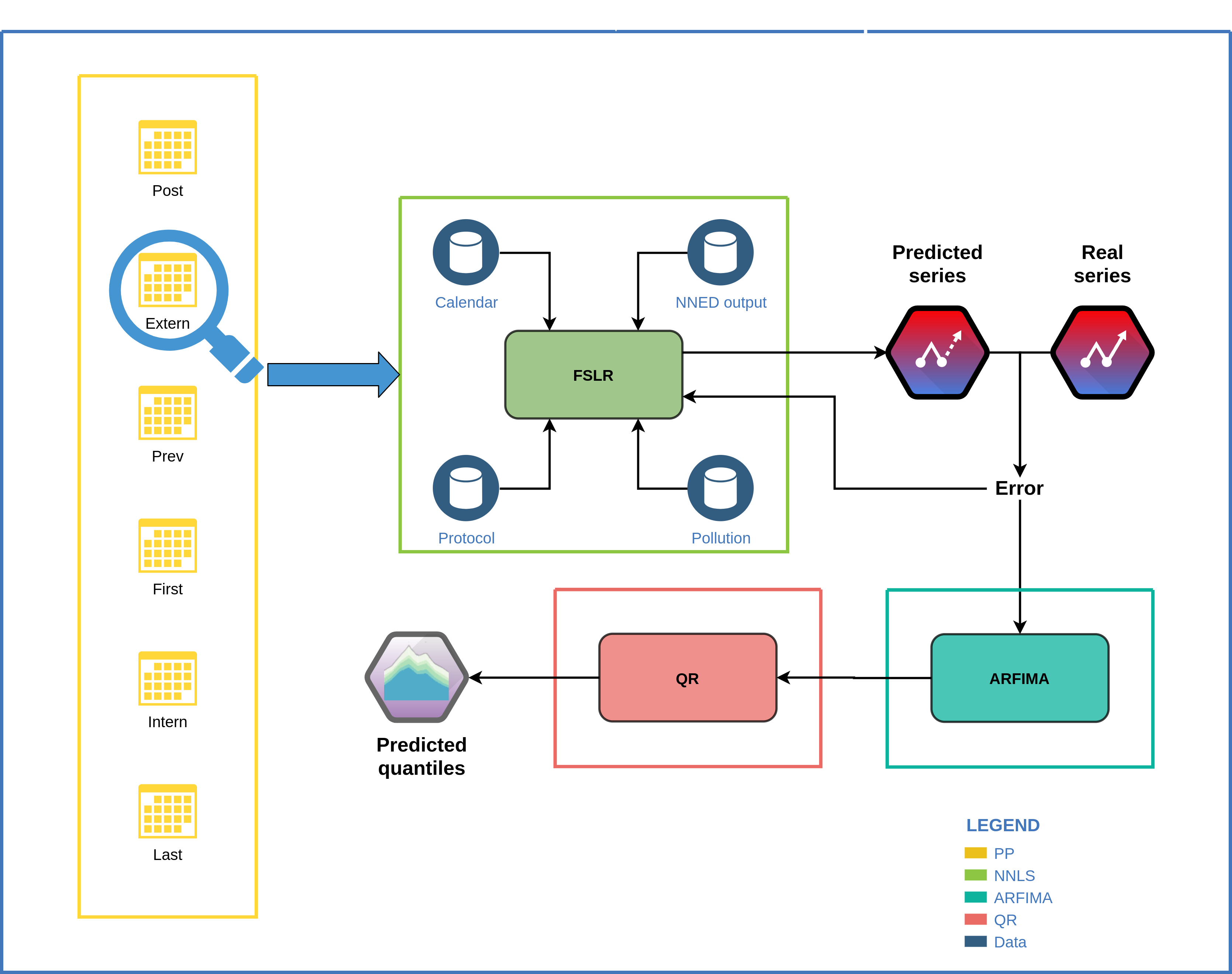
Figure 8: PP-FSLR-ARFIMA-QR scheme. First, input data is classified depending on the type of day to be predicted (yellow). For each new series, the FSLR (green) takes as inputs different data sources (blue). Through linear relations, FSLR models different aspect of the problem, and uses its own prediction error for autoregulation. This same error is fed to the ARFIMA model (sky blue). Finally, the predicted quantiles are computed by the QR (red).

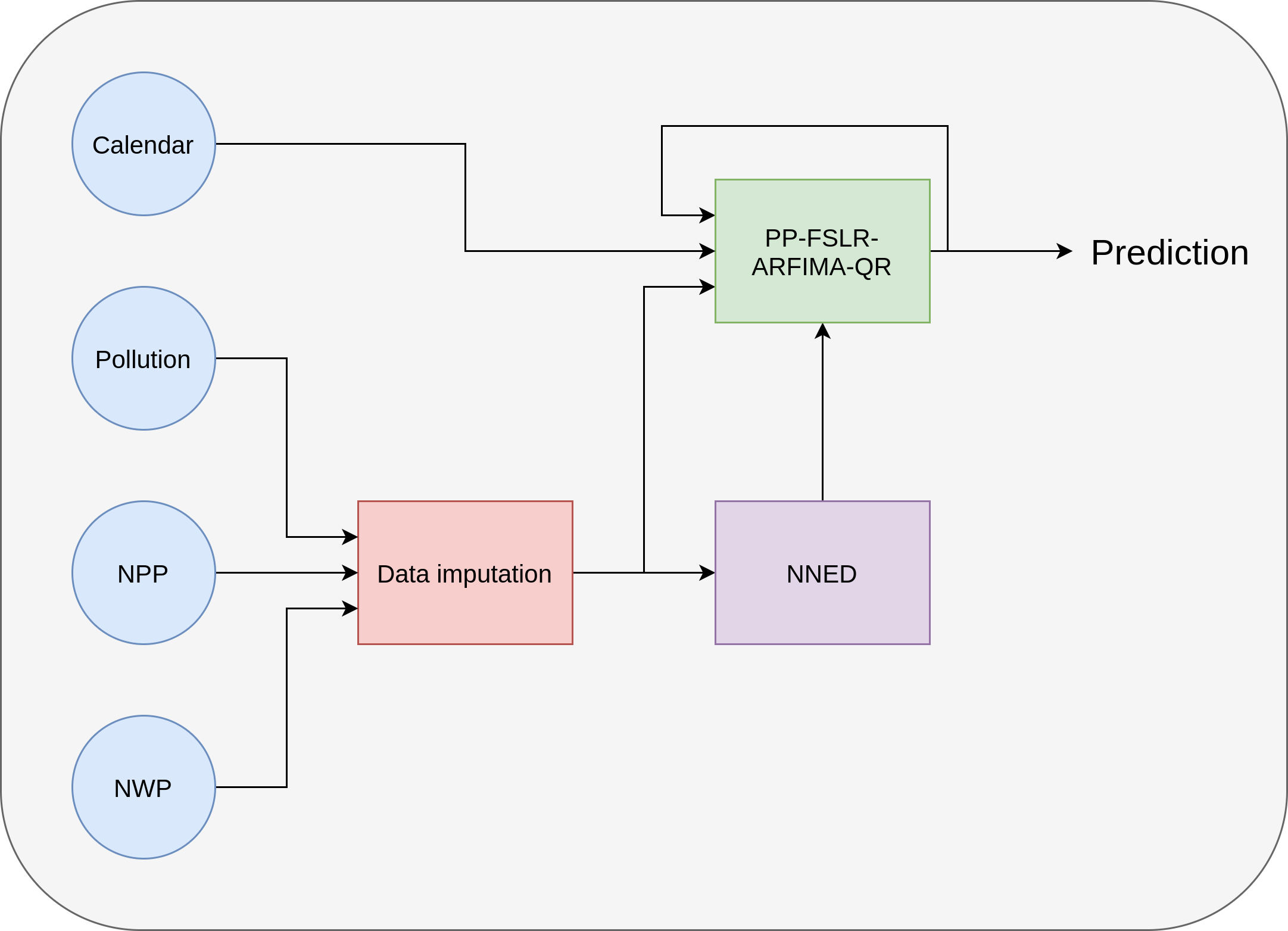
Figure 9: Complete schematic of the ensemble of cascade nested models in SOCAIRE. In blue circles, data sources, and in squares, the mathematical components. The relationships between the different elements of the diagram are reflected by arrows.

At this point, the forecasts generated represent the mathematical expectation of the output magnitudes. With this, one can aspire at most to asymptotically estimate a log-normal distribution under the laws of regression. But since the distribution will not always fit perfectly with a log-normal, it is preferable to use a method based solely on the data.

To do this, a new probabilistic quantile regression (QR) is estimated in order to estimate the future concentrations, with as single input the forecast of the previous FSLR+ARFIMA model, in original terms (without applying the logarithmic transformation), in order to obtain all percentiles from 1% to 99%.

In this setting, since there is not always enough contrast surface (the data-variables ratio is low), it may happen that the estimated percentiles do not comply with the basic rules of non-negative and non-decreasing applicable to every probability distribution. Usually, it is in the extremes where there are more problems. To alleviate this inconsistency, an I-spline interpolation is applied to these percentiles to ensure that these properties are as close as possible to the estimated values.

A general schematic of the PP-FSLR-ARFIMA-QR model is presented in Fig. 8, while Fig. 9 summarises the complete model with the data sources that govern the system.

5 Probabilistic prediction of the alert levels

As described in Section 2.2, the activation of the NO₂ protocol depends on meeting a number of requirements, defined in three alert levels. From a probabilistic point of view, these requirements can be seen as compound events, and being able to compute the future probability for the activation of each level is of utmost importance for decision makers.

According to the NO₂ protocol, the activation of the different levels depends on what happens in several stations at the same time and in a certain number of consecutive hours. In order to compute the aggregated probability, the evaluation of the probability of the intersection of several events is thus needed, knowing only the marginal percentiles and the historical residues left by each of the models.

5.1 Empirical marginal distribution of the different stations

As we have shown above, the model for each station offers a probabilistic forecast condensed in a quantile vector. Specifically, the 99 integer percentiles are taken, that is, those corresponding to the probabilities $p_{k}=1\%,2\%,\dots,98\%,99\%$.

In this section, we will look for a way to calculate the marginal distribution function for the forecast of each pollutant concentration from these quantiles calculated by each station’s model. For this, it will be necessary to calculate the inverse of this distribution function and some statistics such as the mode, which in turn requires an analytical representation that allows us to obtain its first and second derivatives. In summary, we need a pair of easily computable, continuous, and doubly derivable functions that allow us to evaluate very efficiently and precisely approximations of the distribution function and its inverse at any point of their respective domains. The selected method is in fact an empirical change of variable that transforms the concentration into a standardized normal.

We will first take into account the fact that, by definition, the estimated quantiles are evaluations of the change in a variable that transforms the forecasts into a uniform distribution. Although this is valid for any source distribution, for reasons of numerical stability it is preferable to apply the process to the logarithms of the quantiles. Thus, if we apply the inverse of the standard normal distribution function to these log-quantiles, then the values obtained will follow that distribution by construction. Note that the calculation of the mode and deviation becomes trivial in this context.

During the approximation process, we will establish the restriction that the probability density of the concentration forecast is always unimodal, which agrees perfectly with the analyzed observations and the type of models used.

Let us think of the moment in which decision making takes place, $t_{0}$, and let us call $y_{s,t}>0$ the real concentration not yet observed in station $s$ at future instant $t>t_{0}$. The model of the $s$ station will give us the $q_{s,t,k}$ percentiles of the forecast such that $P\left[y_{s,t}\leq q_{s,t,k}\right]=p_{k}$. The transformed values are thus defined as $z_{s,t}=\log\left(y_{s,t}\right)$ and the standardized normal quantile is $u_{k}=\Phi^{-1}_{0,1}\left(p_{k}\right)$, where obviously $\Phi_{0,1}$ is the normal distribution function with mean $0$ and deviation $1$.

Now we will interpolate the pairs $\left(u_{k},z_{t,s}\right)$ by means of a function $f_{s,t}:\mathbb{R}\longrightarrow\mathbb{R}$ that passes through those points

$$f_{s,t}\left(u_{k}\right)=z_{t,s}$$ (4)

and, in an analogous way, the inverse function $g_{s,t}=f_{s,t}^{-1}:\mathbb{R}\longrightarrow\mathbb{R}$ will be constructed as the interpolating function that passes through the points $\left(z_{t,s},u_{k}\right)$. That is to say $g_{s,t}\left(z_{k}\right)=u_{t,s}$.

This allows us to construct an approximation of the concentration distribution function as follows:

$$\Phi_{0,1}\left(g_{s,t}\left(\log\left(y\right)\right)\right)\simeq P\left[y_{s,t}\leq y\right]=\Psi_{s,t}\left(y\right).$$ (5)

And similarly we will obtain the approximation of its inverse:

$$\exp\left(f_{s,t}\left(\Phi_{0,1}^{-1}\left(p\right)\right)\right)\simeq\Psi_{s,t}^{-1}\left(p\right).$$ (6)

Although we could have directly interpolated these functions, which are the true objective, numerically speaking the interpolation with these transformations is more stable (largely because both $z_{s,t}$ and $u_{k}$ are not bounded).

To avoid problems in the tails of the distribution, and taking into account that both functions are monotonous, it is highly recommended to use an interpolation method that guarantees this monotonicity. In particular, a monotonic spline interpolation has been used in this work. The monotony of the functions $f_{s,t}$ and $g_{s,t}$, together with the monotony of the logarithm and the exponential functions, guarantees that the maximum probable value of the concentration will be $\hat{y}_{s,t}=\exp\left(f_{s,t}\left(0\right)\right)$.

Let the standardized residue of the forecast be

$$\varepsilon_{s,t}=g_{s,t}\left(\log\left(y_{s,t}\right)\right)\sim N\left(0,1\right),$$ (7)

and note that indeed, if the probable maximum forecast is exact, i.e. if $y_{s,t}=\hat{y}_{s,t}$, then

$$\varepsilon_{s,t}=g_{s,t}\left(\log\left(\exp\left(f_{s,t}\left(0\right)\right)\right)\right)=g_{s,t}\left(f_{s,t}\left(0\right)\right)=0$$ (8)

Similarly, if the standardized residue is zero, then the forecast is exact.

5.2 Empirical joint distribution

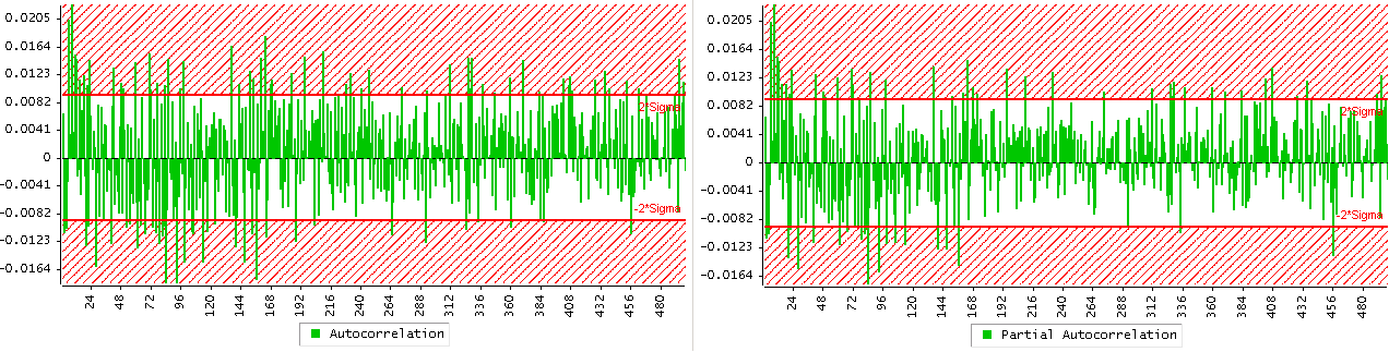
Figure 10: ACF and PACF of residuals in station 58.

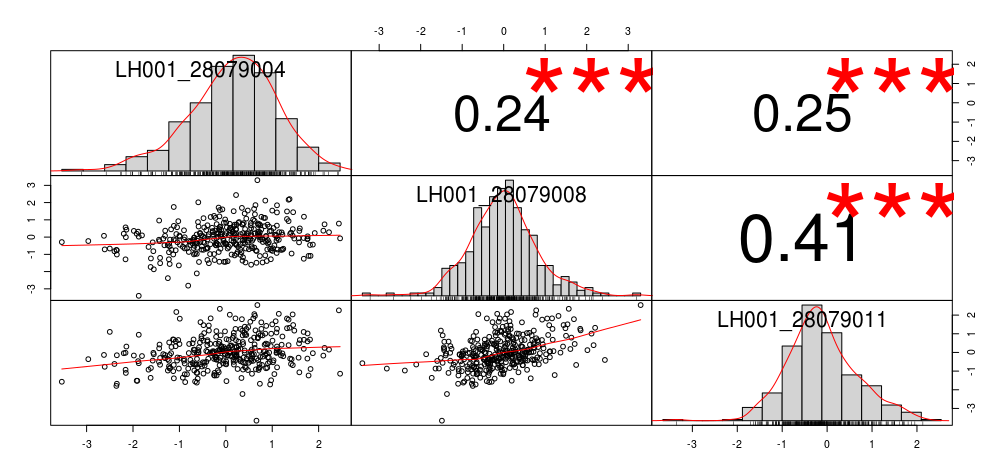
Figure 11: Instantaneous correlations and residual histograms for stations 4, 8 and 11.

Figure 12: Summary of the 1 hour ahead cross-correlations of the residuals series for station 8 and 11.

Section 4 has described the models that marginally predict the concentration of each pollutant at each station for different time horizons. These models, thanks to their ARIMA structure, are able to adequately treat the internal temporal correlation of each station, that is, the autocorrelation of each of the series of pollutants of the different stations. In Fig. 10, it can be seen that the autocorrelation function (ACF) is never too big, and that when it does exceed the 2 sigma limits, so does the partial autocorrelation function (PACF). This fact suggests that these are spurious correlations or any other types of concurrent causes, not linked to time.

However, in view of Fig. 11, there is nothing that indicates that residuals from different stations will be independent of each other. Rather, they appear to correlate.

On the one hand, even if NNED models the spatio-temporal dynamics of the process, it is expected that closer stations will be more similar amongst them, giving rise to positive correlations between their residues. On the other hand, as shown in Fig. 12, the errors in each forecast horizon for a single station will also not be independent of other stations’ previous horizons. In fact, this occurs mostly mutually, present errors of a station correlate with the past errors of another station and vice versa.

In the previous section we have seen how to obtain, by means of an interpolative variable change, standardized normal residues in a marginal way for each station $s$ and for each future instant $t$ at current time $t_{0}$. However, if the independence hypothesis is not plausible it is clear that knowing the marginal distributions does not imply knowing the joint distribution.

A family of models which are naturally capable of dealing with this situation are the X-VecARMA , a type of multivariate models [34] that include exogenous inputs, cointegration, and vector ARMA. They are considered very powerful for the representation of cross-correlated vector processes that might include exogenous factors eventually shared by several of them. However, they are intractable in computational terms for this setting.

Thus, we propose an empirical multi-normal copula [29] to approximate the joint distribution for every station and horizon. The aim is to obtain an estimate of such joint distribution function for all the forecasts obtained marginally, both in time and space, using the joint sample correlation matrix between each pair of stations among all the horizons and stations.

However, since there are $48$ horizons and $24$ stations, that gives us a square matrix of $1152$ rows, and we would need at least $10$ years of forecasts to obtain a meager $3$ to $1$ response surface, which is clearly unacceptable. For this reason, we have developed a boxed tridiagonal scheme, in which correlations are only taken into account one period ahead. With this scheme, only one year of forecasting is sufficient to obtain a reasonable estimate.

We will assume that the joint distributions of these standardized residues only depend on the station and the forecast horizons $h=t-t_{0}$ and $h-1=t-1-t_{0}$, but not on the specific moment $t$, since the forecasts will be made every day at the same time.

Since the marginal distributions of all the $\varepsilon_{1,t}$ are normal, unbiased and with unit variance, the joint distribution of all stations,

$$\varepsilon_{h}=\left(\varepsilon_{1,t_{0}+h},\cdots,\varepsilon_{s,t_{0}+h},\cdots,\varepsilon_{S,t_{0}+h}\right)^{T}\in\mathbb{R}^{S},$$ (9)

will be an unbiased multinormal with an unknown but obligatory unitary covariance matrix, that is, equal to the correlation matrix. In the same way we will suppose that the residuals $\left(\varepsilon_{h-1},\varepsilon_{h}\right)$ corresponding to each pair of consecutive horizons are also distributed the same way.

By the principle of causality, for the previous horizon, $\varepsilon_{h-1}$, an independent distribution of the following $\varepsilon_{h-1}$ will be postulated, since future events cannot influence the past. In this way, we can define the joint distribution of the different stations in each horizon in a recursive way:

$$\begin{array}[]{c}\varepsilon_{1}\sim\mathcal{N}(0,C_{1})\\ \left(\varepsilon_{h-1},\varepsilon_{h}\right)\sim\mathcal{N}(0,C_{h}),\forall h=2,3,\ldots,H\\ C_{h}=\left(\begin{array}[]{ll}C_{h-1,h-1}&C_{h-1,h}\\ C_{h-1,h}^{T}&C_{h,h}\end{array}\right)\in\mathbb{R}^{2S\times 2S},\forall h=2,3,\ldots,H\\ C_{1}=C_{1,1},C_{h-1,h},C_{h,h}\in\mathbb{R}^{S\times S}\\ C_{h-1,h-1,s,s}=C_{h,h,s,s}=1\\ C_{h,h,s,s^{\prime}}=\rho_{\varepsilon_{s,t_{0}+h},\varepsilon_{s^{\prime},t_{0}+h}}\in\left(-1,1\right)\\ C_{h-1,h,s,s^{\prime}}=\rho_{\varepsilon_{s,t_{0}+h-1},\varepsilon_{s^{\prime},t_{0}+h}}\in\left(-1,1\right)\end{array}$$ (10)

Note that the joint distribution of all horizons would have a tridiagonal covariance matrix with partitions of order $S$:

$$\mathrm{C}=\left(\begin{array}[]{cccc}C_{1,1}&C_{1,2}&&0\\ C_{1,2}^{T}&\ddots&\ddots\\ &\ddots&\ddots&C_{H-1,H}\\ 0&&C_{H-1,H}^{T}&C_{H,H}\end{array}\right).$$ (11)

If we calculate the forecasts for enough dates $t_{0}$ of the past, at the same time of the day and with the same horizons $h=1,2,\dots,H$, we can obtain many samples of the residues with which we can thus estimate the matrices $C_{h-1,h}$ and $C_{h,h}$. In this way, we would obtain the distributions for each horizon conditioned on the previous horizon, using the formula known analytically for the conditional partitioned multivariate normal:

$$\left.\begin{array}[]{c}\varepsilon_{h}\sim\mathcal{N}\left(\mu_{h},C^{\prime}_{h}\right)\\ \mu_{h}=C_{h-1,h}^{T}C_{h-1,h-1}^{-1}\varepsilon_{h-1}\in\mathbb{R}^{S}\\ C^{\prime}_{h}=C_{h,h}-C_{h-1,h}^{T}C_{h-1,h-1}^{-1}C_{h-1,h}\in\mathbb{R}^{S\times S}\end{array}\right\}\forall h=2,3,\ldots,H$$ (12)

These matrices can be stored for later use in future joint forecasts, along with their Cholesky and inverse decompositions:

$$\begin{array}[]{c}C_{h,h}=L_{h}L_{h}^{T},\;\forall h=1,2,3,\ldots,H\\ C^{\prime}_{h}=L^{\prime}_{h}L^{\prime T}_{h},\;\forall h=2,3,\ldots,H\end{array}$$ (13)

First we simulate $N$ vectors of $N$ standardized independent residuals for the first horizon

$$\eta_{1,n}\sim\mathcal{N}\left(0,I\right),\forall n=1,2,\ldots,N$$ (14)

and pre-multiplying them by $L_{1}$ we will have the standardized residuals of all the stations for the first horizon:

$$\varepsilon_{1,n}=L_{1}\eta_{1,n}\sim\mathcal{N}\left(0,C_{1}\right).$$ (15)

From there, also starting from independent residuals

$$\eta_{h,n}\sim\mathcal{N}\left(0,I\right),\forall n=1,2,\ldots,N,$$ (16)

residuals of each horizon conditioned by the previous one can be simulated:

$$\varepsilon_{h}=\mu_{h}+L_{h}^{\prime}\eta_{h,n}.$$ (17)

On the one hand, this approach solves the problem of time correlation in consecutive hours, which is what is required, and on the other hand it is simple enough to be able to generate correct estimations.

Finally, applying the transformations detailed Section 5.2 we obtain $N$ realizations of the future forecasts of the concentrations of the different stations in each horizon:

$$y_{s,t_{0}+h,n}=\exp\left(f_{s,t}\left(\varepsilon_{s,h,n}\right)\right).$$ (18)

If this simulation is repeated a sufficient number of times we can calculate any joint statistic from the forecasts of the concentrations in the different stations. In particular, for example, to calculate the probability of activation of the pre-warning level of the NO₂ protocol, defined as the probability of the concentration of NO₂ exceeding a certain threshold $\varUpsilon=180$ in at least two stations during two consecutive hours, it will simply be necessary to calculate what proportion of the simulated samples meet these criteria.

6 Operation and performance

6.1 Operation

Figure 13: Main page of the SOCAIRE web app for controlling and monitoring pollution in the city of Madrid.

(a) Prewarning.

(b) Warning.

(c) Alert.

Figure 14: Probability of activation for the three levels of the NO₂ protocol, predicted the 29/09/2020.

(a) NO₂.

(b) O₃.

(c) PM$10$.

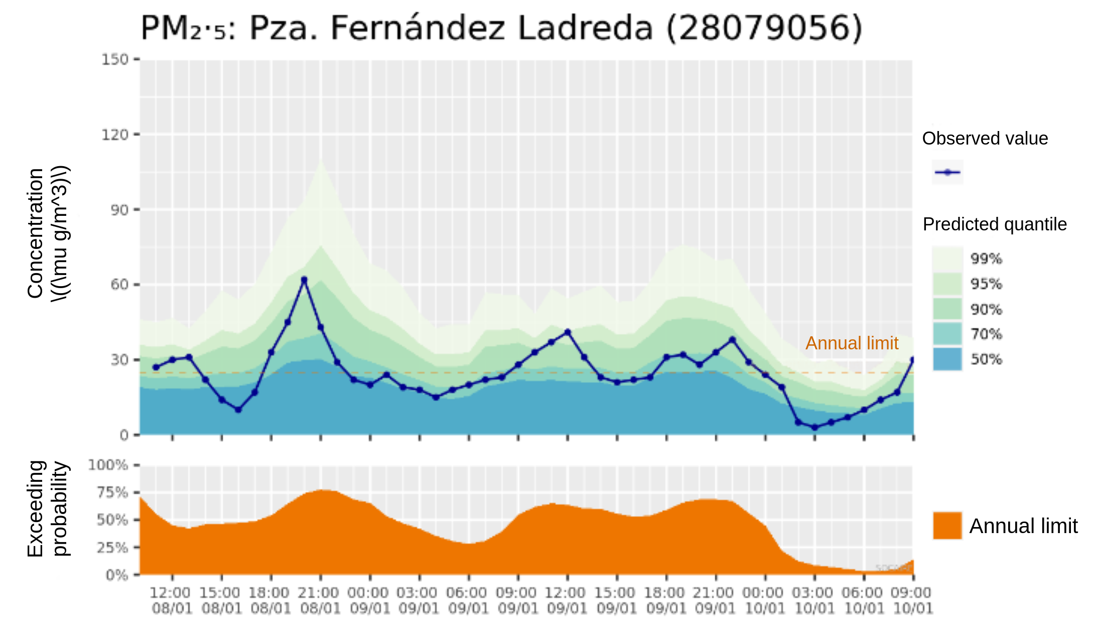
(d) PM$2.5$.

Figure 15: Forecast quantile and probabilities of exceedance for each hour in station 56 for 08/01/2020. The real observed values are represented by the blue lines and dots and, thus, it is possible to have a reference about SOCAIRE performance (which will be covered in Section 6.2).

In order to be used by decision makers in the department of the city council in charge of air quality, SOCAIRE has been integrated with a web app that allows to simply and directly view the forecasts for pollutants and the probability of reaching the levels established within the NO₂ protocol as explained in section 2.2. This section will show the site structure and its basic operation principles.

The main overview of the web tool is shown in Fig. 13. On the one hand, at the top you can choose the pollutant to display (blue buttons), the date on which you want to make a query (calendar button), and different submenus where you can see in more detail the probability that the protocol will be activated (shown tab), and both the system predictions and a summary of contrast measures. On the other hand, in the central part the information related to the submenu in which the user is at that moment is shown. In this specific case, the probability of the levels of the NO₂ protocol being activated.

The operation of the tool for monitoring the future probability of reaching the different levels of the protocol are presented in Fig. 14. After using the ensemble of nested models described in Section 4 to forecast NO₂ quantiles, the outer rings show the probability of each individual station exceeding the levels set in the NO₂ protocol (180 $\mathrm{\mu g/m^{3}}$, 200 $\mathrm{\mu g/m^{3}}$, and 400 $\mathrm{\mu g/m^{3}}$ for prewarning, warning, and alert respectively). Once the individual probabilities are computed, it is possible to use the process explained through Section 5 to estimate probabilities of compound events. Given that the protocol is defined over areas and not for individual station levels, the intermediate ring shows the probability of exceeding the expected pollution levels for each of the 5 areas in which Madrid is partitioned in the NO₂ protocol (see Fig. 1(b)). Lastly, the inner ring contains the aggregated probability of the different levels of the protocol being activated in the entire city. It uses the probabilities over the five areas to estimate this final probability.

Since the set of mobility measures defined in the NO₂ protocol depends on reaching extreme levels in various stations and for a pre-set number of consecutive hours, having such an overview is especially important. However, it is also interesting to visualize the individual forecast for each station over time. The SOCAIRE website allows viewing the actual forecasts for each pollutant and each station, as shown in Fig. 15. Together with the predicted quantiles and real observed values, these plots also show the probability of exceeding each level and the levels themselves.

6.2 Performance analysis

Table 2: Average error for $t=1$ to $t=48$, calculated over all stations. For a more detailed view of error metrics distribution, see Fig. 16.

	NO2		$O_{3}$		$PM10$		$PM2.5$
	RMSE	Bias	RMSE	Bias	RMSE	Bias	RMSE	Bias
CAMS	$23.5\pm 9.1$	$12.3\pm 9.8$	$19.1\pm 5.0$	$-3.2\pm 6.2$	$13.9\pm 3.7$	$6.3\pm 3.7$	$6.5\pm 1.3$	$1.1\pm 2.1$
Persistence	$26.4\pm 9.3$	$-1.4\pm 3.5$	$27.4\pm 4.8$	$0.5\pm 16.0$	$15.5\pm 3.1$	$-0.6\pm 3.5$	$7.8\pm 1.4$	$-0.3\pm 1.4$
SOCAIRE	$14.9\pm 4.8$	$-0.2\pm 0.8$	$15.8\pm 2.8$	$1.6\pm 1.0$	$10.6\pm 2.5$	$0.3\pm 0.7$	$5.4\pm 1.0$	$-0.1\pm 0.65$

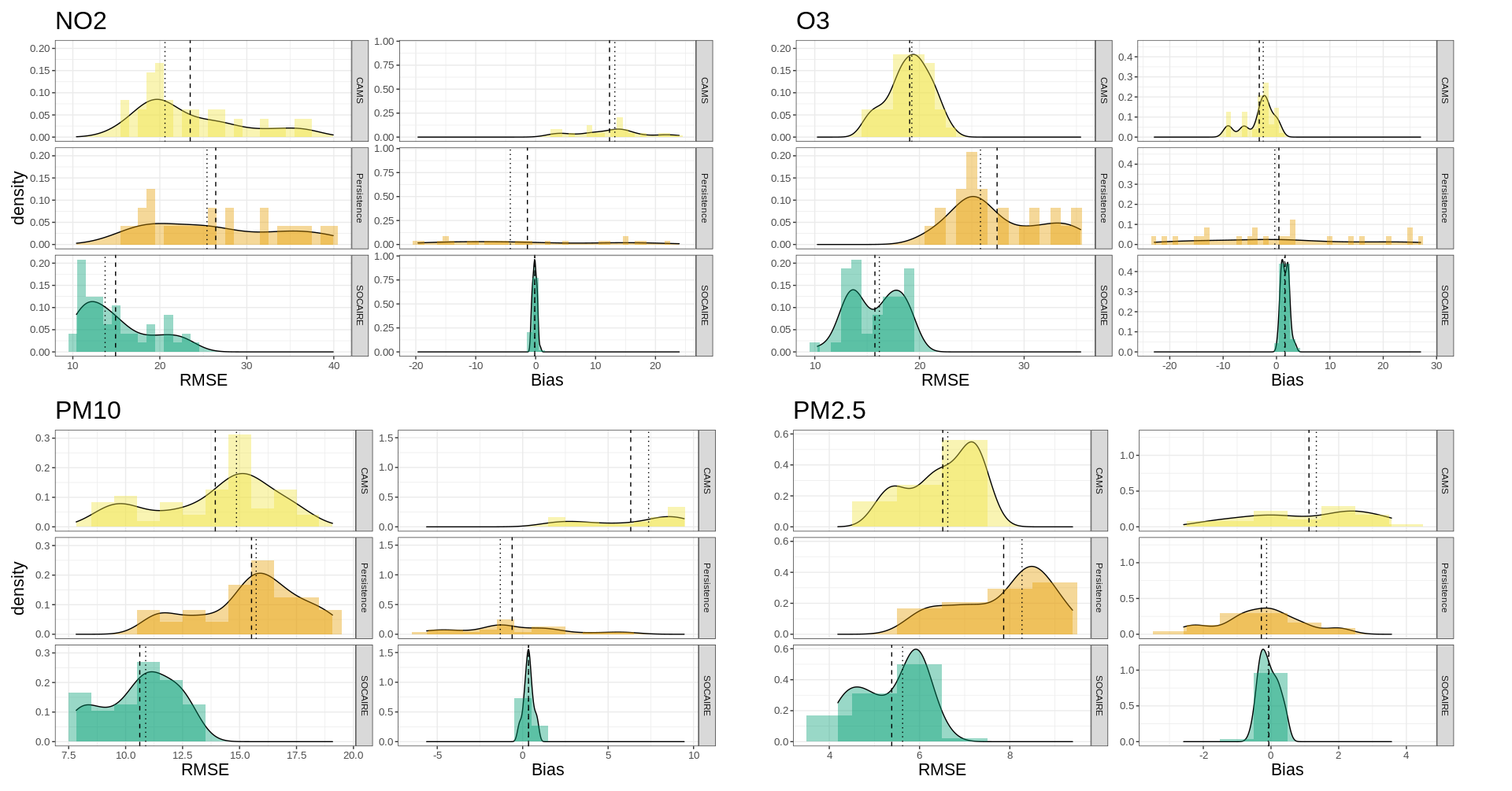
Figure 16: Error distribution for the four pollutants in terms of RMSE and bias. Dashed vertical line represents the mean, dotted vertical line represents the median.

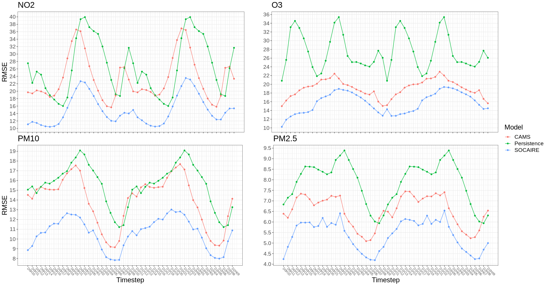
Figure 17: RMSE error by timestep. D makes reference to the day and H to the hour (D0H10 means day 0 or present day at 10:00).

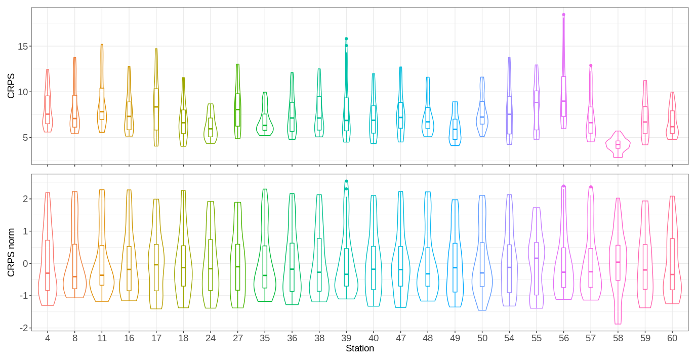
Figure 18: Comparison of the error distribution for all stations (top). Scaling CRPS to a $\mathcal{N}(0,1)$ let us conclude that all stations have been correctly modeled in the spatial dimension (bottom).

Usual error metrics, as RMSE, refer to expected values, which are found in the central part of the distribution, but do not take into account any other information, and are thus particularly unfit to evaluate probabilistic forecasts. Since the most usual models produce point forecasts and not the entire distribution, these kinds of metrics are the only option. However, when dealing with the prediction of the complete distribution as in our case, other metrics have been proposed in order to summarise model performance information in a more comprehensive and realistic way. For example, CRPS is a measure of the squared difference between the forecast cumulative distribution function (CDF) and the empirical CDF of the observation [10].

As we will show, in terms of performance SOCAIRE compares favorably to benchmarks. In order to get a clear and quick idea about the behavior of the model, Table 2 shows the RMSE and bias (averaged both in time and space) of the proposed methodology and compares it with two other models that, due to their characteristics, make it easier to understand the real performance of SOCAIRE: persistence and the NPP provided by CAMS.

The persistence model is a naive model in which the forecast value is taken to be the observed value at the previous timestep. It is, thus, a good benchmark model and one can get a rough idea of how good a new model is by seeing how much improvement there is with respect to persistence. In our specific case, for contractual reasons, we use a more elaborated version of persistence which includes the daily, weekly, and annual cyclical structure of the series, and is thus a simple although powerful model.

Similarly, the NPP provided by CAMS represent another good baseline to be improved upon by any new model. Since it is based on a synoptic scale, it is expected that any model focused on a smaller and concrete terrain extension will improve its results. If this is not the case, it would make more sense to use CAMS NPP as an approximation instead of the proposed new methodology.

For a more detailed view of error metrics, refer to Fig. 16. As it can be seen, SOCAIRE consistently outperforms both baselines in terms of RMSE and bias for the four pollutants. Concretely, SOCAIRE supposes an average RMSE improving of $32\%$ with respect to CAMS and $60\%$ with respect to persistence, reinforcing the idea that SOCAIRE shows good performance and behaves very well as a predictor. Also, SOCAIRE demonstrates to be in general terms an unbiased predictor of pollution, which emphasizes the fact that the proposed model is being able to correctly describe the aforementioned terms related to the system.

Another issue that is of special importance in our problem is the behavior of the model depending on the prediction timestep/hour. As it was shown in Fig. 3, the series are highly hour-dependent. For example, NO₂ presents peaks usually around 08:00–10:00 and 22:00–00:00. In the framework of air quality management and monitoring, these peaks are extremely important as they represent the higher risk and, consequently, the moments when the maximum recommended and/or permitted levels are usually exceeded. Thus, and given that one of the main objectives of SOCAIRE framework is forecasting the probability of each level of the NO₂ protocol, showing a good performance in peak hours is of crucial importance.

Fig. 17 presents the RMSE error for each pollutant and for each prediction horizon averaged over all stations. From this figure, it becomes clear that SOCAIRE is especially efficient in peak hours, where the gap with baseline models is even wider.

Until now, we have covered aggregated error over all stations. As the activation of the NO₂ protocol depends on compound events of individual stations, it is important to make sure all of them behave similarly. As it was explained before, the complete model has a module which is able to relate and exploit shared spatial information (Section 4.2), but it also models each station independently based on its own characteristics (Section 4.3). By taking into account both types of information, we expect to avoid possible biases of predominance by some spatial areas over others but still be able to make use of the relations that exist among them. The CRPS for the NO₂ predictions at each station is shown in the top row of Fig. 18. It is worth noting that stations with lower CRPS errors correspond to green areas of the city of Madrid (Stations 24, 49, and 58). Scaling these CRPS values to a $\mathcal{N}(0,1)$ (bottom row of Fig. 18) let us see how all error distributions have a very similar behavior. Hence, it is possible to assure that our modeling strategy works as expected and results in an approximately unbiased prediction of the spatial component.

7 Conclusions and future work

Throughout this manuscript, we have discussed the details of SOCAIRE, the new operational system for air quality forecasting and monitoring in the city of Madrid. Based on an ensemble of statistical and neural models, SOCAIRE is built under the premise that it is possible to integrate the diverse information that correlates with air quality in order to model it. This information includes historical values of the series itself, numerical weather and pollution predictions, and anthropogenic features. Concretely, the proposed methodology tackles the prediction of the four main pollutants (NO₂, O₃, PM10, and PM2.5) for a 48-hour horizon. Thanks to its probabilistic nature, the system is able to combine the predictions of the full probability distribution for compound events using a Bayesian estimation of the future distribution of the different stations over time. Thus, the system outputs are a valuable tool for managing the NO₂ protocol enforced by the city council of Madrid.

The tool presented in this paper is not only a theoretical proposal, but it has been adopted as the official application to monitor, analyze and make day-to-day decisions about air quality. The last part of this work summarizes the structure and operation of SOCAIRE’s web, as well as the main highlights of the good results and performance of the system.

In the future, it would be interesting to apply a cost-efectiveness analysis focused on the NO₂ protocol activation probability. Also, we are working towards the inclusion of a traffic forecasting system, which might improve the performance of the models by enhancing the information that anthropogenic features provide. Finally, SOCAIRE could be adapted to predict any kind of combined air quality index, and not only those ones affecting the current protocol.

8 Acknowledgments

The authors would like to thank José Amador Fernández Viejo and the team at the General Directorate for Sustainability of the Municipality of Madrid, especially María de los Ángeles Cristóbal López for her continuing support and enthousiasm towards this project.

This research has been partially funded by Empresa Municipal de Transportes (EMT) of Madrid, Spain under the program "Aula Universitaria EMT/UNED de Calidad del Aire y Movilidad Sostenible".

References

- [1] José L. Aznarte “Probabilistic forecasting for extreme NO2 pollution episodes” In Environmental Pollution 229, 2017, pp. 321–328 DOI: 10.1016/j.envpol.2017.05.079
- [2] Artur J. Badyda, James Grellier and Piotr Dąbrowiecki “Ambient PM2.5 Exposure and Mortality Due to Lung Cancer and Cardiopulmonary Diseases in Polish Cities” In Advances in Experimental Medicine and Biology 944, 2017, pp. 9–17 DOI: 10.1007/5584_2016_55
- [3] Lu Bai, Jianzhou Wang, Xuejiao Ma and Haiyan Lu “Air Pollution Forecasts: An Overview” In International Journal of Environmental Research and Public Health 15.4, 2018 DOI: 10.3390/ijerph15040780
- [4] Helene Blanchonnet “Set I - Atmospheric Model high resolution 10-day forecast (HRES)” Library Catalog: www.ecmwf.int In ECMWF, 2015 URL: https://www.ecmwf.int/en/forecasts/datasets/set-i
- [5] George EP Box, Gwilym M Jenkins, Gregory C Reinsel and Greta M Ljung “Time series analysis: forecasting and control” John Wiley & Sons, 1976
- [6] Leo Breiman “Statistical Modeling: The Two Cultures (with comments and a rejoinder by the author)” In Statist. Sci. 16.3 The Institute of Mathematical Statistics, 2001, pp. 199–231 DOI: 10.1214/ss/1009213726
- [7] “Copernicus air quality monitoring” In euronews URL: https://atmosphere.copernicus.eu/
- [8] “En portada - Portal de datos abiertos del Ayuntamiento de Madrid” URL: https://datos.madrid.es/portal/site/egob
- [9] Daniel Fink “A Compendium of Conjugate Priors”, 1997
- [10] Tilmann Gneiting and Matthias Katzfuss “Probabilistic Forecasting” _eprint: https://doi.org/10.1146/annurev-statistics-062713-085831 In Annual Review of Statistics and Its Application 1.1, 2014, pp. 125–151 DOI: 10.1146/annurev-statistics-062713-085831
- [11] C… Granger and Roselyne Joyeux “An Introduction to Long-Memory Time Series Models and Fractional Differencing” _eprint: https://onlinelibrary.wiley.com/doi/pdf/10.1111/j.1467-9892.1980.tb00297.x In Journal of Time Series Analysis 1.1, 1980, pp. 15–29 DOI: https://doi.org/10.1111/j.1467-9892.1980.tb00297.x
- [12] G. Grivas and A. Chaloulakou “Artificial neural network models for prediction of PM10 hourly concentrations, in the Greater Area of Athens, Greece” In Atmospheric Environment 40.7, 2006, pp. 1216–1229 DOI: 10.1016/j.atmosenv.2005.10.036
- [13] S. Hassanzadeh, F. Hosseinibalam and R. Alizadeh “Statistical models and time series forecasting of sulfur dioxide: a case study Tehran” In Environmental Monitoring and Assessment 155.1-4, 2009, pp. 149–155 DOI: 10.1007/s10661-008-0424-1
- [14] Marie-Eve Héroux et al. “Quantifying the health impacts of ambient air pollutants: recommendations of a WHO/Europe project” In International Journal of Public Health 60.5, 2015, pp. 619–627 DOI: 10.1007/s00038-015-0690-y
- [15] Rob J Hyndman and Yeasmin Khandakar “Automatic time series forecasting: the forecast package for R” In Journal of Statistical Software 26.3, 2008, pp. 1–22 URL: https://www.jstatsoft.org/article/view/v027i03
- [16] Frank E. Jr “Hmisc: Harrell Miscellaneous”, 2020 URL: https://CRAN.R-project.org/package=Hmisc
- [17] Egide Kalisa et al. “Temperature and air pollution relationship during heatwaves in Birmingham, UK” In Sustainable Cities and Society 43, 2018, pp. 111–120 DOI: 10.1016/j.scs.2018.08.033
- [18] Ki-Hyun Kim, Ehsanul Kabir and Shamin Kabir “A review on the human health impact of airborne particulate matter” In Environment International 74, 2015, pp. 136–143 DOI: 10.1016/j.envint.2014.10.005
- [19] Kyung Hwan Kim, Seung-Bok Lee, Daekwang Woo and Gwi-Nam Bae “Influence of wind direction and speed on the transport of particle-bound PAHs in a roadway environment” In Atmospheric Pollution Research 6.6, 2015, pp. 1024–1034 DOI: 10.1016/j.apr.2015.05.007
- [20] Ujjwal Kumar and V.. Jain “ARIMA forecasting of ambient air pollutants (O3, NO, NO2 and CO)” In Stochastic Environmental Research and Risk Assessment 24.5, 2010, pp. 751–760 DOI: 10.1007/s00477-009-0361-8
- [21] Charles L Lawson and Richard J Hanson “Solving least squares problems” SIAM, 1995
- [22] Piotr S. Maciąg, Nikola Kasabov, Marzena Kryszkiewicz and Robert Bembenik “Air pollution prediction with clustering-based ensemble of evolving spiking neural networks and a case study for London area” In Environmental Modelling & Software 118, 2019, pp. 262–280 DOI: 10.1016/j.envsoft.2019.04.012
- [23] V. Marécal et al. “A regional air quality forecasting system over Europe: the MACC-II daily ensemble production” Publisher: Copernicus GmbH In Geoscientific Model Development 8.9, 2015, pp. 2777–2813 DOI: https://doi.org/10.5194/gmd-8-2777-2015
- [24] Marco Martuzzi, Francesco Mitis, IVANO Iavarone and Maria Serinelli “Health impact of PM10 and ozone in 13 Italian cities” In WHO Regional Office for Europe, 2006, pp. 133
- [25] Rodrigo Medrano and José L. Aznarte “On the Inclusion of Spatial Information for Spatio-Temporal Neural Networks” arXiv: 2007.07559 In arXiv:2007.07559 [cs, stat], 2020
- [26] Agencia Estatal de Meteorología “Agencia Estatal de Meteorología - AEMET. Gobierno de España” URL: http://www.aemet.es/es/portada
- [27] Ricardo Navares and José L. Aznarte “Predicting air quality with deep learning LSTM: Towards comprehensive models” In Ecological Informatics 55, 2020, pp. 101019 DOI: 10.1016/j.ecoinf.2019.101019
- [28] Asaf Nebenzal and Barak Fishbain “Long-term forecasting of nitrogen dioxide ambient levels in metropolitan areas using the discrete-time Markov model” In Environmental Modelling & Software 107, 2018, pp. 175–185 DOI: 10.1016/j.envsoft.2018.06.001
- [29] Roger B. Nelsen “An Introduction to Copulas”, Lecture Notes in Statistics New York: Springer-Verlag, 1999 DOI: 10.1007/978-1-4757-3076-0
- [30] Wei Ouyang et al. “The washing effect of precipitation on particulate matter and the pollution dynamics of rainwater in downtown Beijing” In Science of The Total Environment 505, 2015, pp. 306–314 DOI: 10.1016/j.scitotenv.2014.09.062
- [31] Halûk Özkaynak et al. “Summary and findings of the EPA and CDC symposium on air pollution exposure and health” In Journal of exposure science & environmental epidemiology 19.1 Nature Publishing Group, 2009, pp. 19–29
- [32] “Protocolo de actuación para episodios de contaminación por dióxido de nitrógeno - Ayuntamiento de Madrid”, 2018 URL: https://www.madrid.es/portales/munimadrid/es/Inicio/Medidas-especiales-de-movilidad/Protocolo-de-contaminacion/Protocolo-de-actuacion-para-episodios-de-contaminacion-por-dioxido-de-nitrogeno/?vgnextfmt=default&vgnextoid=fd8718cea863c410VgnVCM1000000b205a0aRCRD&vgnextchannel=00b3cf7588c97610VgnVCM2000001f4a900aRCRD
- [33] Yann Sellier et al. “Health effects of ambient air pollution: Do different methods for estimating exposure lead to different results?” In Environment International 66, 2014, pp. 165–173 DOI: 10.1016/j.envint.2014.02.001
- [34] Christopher A Sims “Macroeconomics and reality” In Econometrica: journal of the Econometric Society JSTOR, 1980, pp. 1–48
- [35] M. Thatcher and P. Hurley “A customisable downscaling approach for local-scale meteorological and air pollution forecasting: Performance evaluation for a year of urban meteorological forecasts” In Environmental Modelling & Software 25.1, 2010, pp. 82–92 DOI: 10.1016/j.envsoft.2009.07.014
- [36] PEAN UNION “Directive 2008/50/EC of the European Parliament and of the Council of 21 May 2008 on ambient air quality and cleaner air for Europe” In Official Journal of the European Union, 2008
- [37] María Vega García and José L. Aznarte “Shapley additive explanations for NO2 forecasting” In Ecological Informatics 56, 2020, pp. 101039 DOI: 10.1016/j.ecoinf.2019.101039