Metric theory of Weyl sums

Abstract.

We prove that there exist positive constants $C$ and $c$ such that for any integer $d\geqslant 2$ the set of $\mathbf{x}\in[0,1)^{d}$ satisfying

$$cN^{1/2}\leqslant\left|\sum_{n=1}^{N}\exp\left(2\pi i\left(x_{1}n+\ldots+x_{d}n^{d}\right)\right)\right|\leqslant CN^{1/2}$$

for infinitely many natural numbers $N$ is of full Lebesque measure. This substantially improves the previous results where similar sets have been measured in terms of the Hausdorff dimension. We also obtain similar bounds for exponential sums with monomials $xn^{d}$ when $d\neq 4$. Finally, we obtain lower bounds for the Hausdorff dimension of large values of general exponential polynomials.

1. Introduction

1.1. Background and motivation

For an integer $d\geqslant 1$, let

$$\mathsf{T}_{d}=({\mathbb{R}}/{\mathbb{Z}})^{d}$$

be the $d$-dimensional unit torus. When $d=1$ we write

$$\mathsf{T}=\mathsf{T}_{1}={\mathbb{R}}/{\mathbb{Z}}.$$

For a vector $\mathbf{x}=(x_{1},\ldots,x_{d})\in\mathsf{T}_{d}$ and integer $N,$ we consider the exponential sums

$$S_{d}(\mathbf{x};N)=\sum_{n=1}^{N}{\mathbf{\,e}}\left(x_{1}n+\ldots+x_{d}n^{d}\right),$$

which are commonly called Weyl sums, where throughout the paper we denote ${\mathbf{\,e}}(x)=\exp(2\pi ix)$. These sums were originally introduced by Weyl to study equidistribution of fractional parts of polynomials and rose to prominence through applications to the circle method and Riemann zeta function. Despite more than a century since these sums were introduced, their behaviour for individual values of $\mathbf{x}$ is not well understood, see [7, 8].

Much more is known about the average behaviour of $S_{d}(\mathbf{x};N)$. The recent advances of Bourgain, Demeter and Guth [3] (for $d\geqslant 4$) and Wooley [39] (for $d=3$) (see also [41]) for the Vinogradov mean value theorem imply the estimate

(1.1) $$N^{s(d)}\leqslant\int_{\mathsf{T}_{d}}|S_{d}(\mathbf{x};N)|^{2s(d)}d\mathbf{x}\leqslant N^{s(d)+o(1)},$$

where

$$s(d)=\frac{d(d+1)}{2}$$

and is best possible up to $o(1)$ in the exponent of $N$.

We observe that the optimal bound (1.1) does not tell much about the typical size of sums $S_{d}(\mathbf{x};N)$. It is conceivable, however unlikely, that the average value is influenced by a very small set of $\mathbf{x}\in\mathsf{T}_{d}$, while for other $\mathbf{x}\in\mathsf{T}_{d}$ these sums are very small. The main goal of this paper is to rule out this possibility and show that for almost all $\mathbf{x}\in\mathsf{T}_{d}$ the sums $S_{d}(\mathbf{x};N)$ have order corresponding to the average size $N^{1/2}$ for infinitely many $N$.

1.2. Previous results and questions

The first results concerning the metric behaviour of Weyl sums are due to Hardy and Littlewood [21] who have estimated the Gauss sums

(1.2) $$G(x;N)=\sum_{n=1}^{N}{\mathbf{\,e}}\left(xn^{2}\right),$$

in terms of the continued fraction expansion of $x$. This idea has been expanded upon by Fiedler, Jurkat and Körner [19, Theorem 2] who give the following optimal lower and upper bounds. Suppose that $\{f(n)\}_{n=1}^{\infty}$ is a non-decreasing sequence of positive numbers. Then one has

(1.3) $$\begin{split}\operatorname*{\overline{lim}}_{N\to\infty}\frac{\left|G(x;N)\right|}{\sqrt{N}f(N)}<\infty&\text{ for almost all }x\in\mathsf{T}\\ &\qquad\Longleftrightarrow\quad\sum_{n=1}^{\infty}\frac{1}{nf(n)^{4}}<\infty.\end{split}$$

See also [17, Theorem 0.1] for similar results with the more general sums $S_{2}(\mathbf{x};N)$, (which correspond to $G(x;N)$ with a linear term in the phase).

For $d\geqslant 3$, it has been shown that for almost all $\mathbf{x}\in\mathsf{T}_{d}$

$$|S_{d}(\mathbf{x};N)|\leqslant N^{1/2+o(1)},\qquad N\rightarrow\infty.$$

It has also been conjectured that the exponent $1/2$ is best possible, see [10, Conjecture 1.1]. In this paper, among other things we confirm this conjecture, see Theorem 2.3 below.

For $\alpha\in(0,1)$ and integer $d\geqslant 2$, consider the set

$$\mathscr{E}_{d,\alpha}=\{\mathbf{x}\in\mathsf{T}_{d}:\leavevmode\nobreak\ |S_{d}(\mathbf{x};N)|\geqslant N^{\alpha}\text{ for infinity many }N\in{\mathbb{N}}\}.$$

We remark that in the series of works [10, 12, 11] for any $\alpha\in(0,1)$ some upper and lower bounds have been given on the Hausdorff dimension $\dim\mathscr{E}_{d,\alpha}$ of $\mathscr{E}_{d,\alpha}$ (see Definition 2.5 below).

In Section 8 we present some heuristic arguments about the exact behaviour of $\dim\mathscr{E}_{d,\alpha}$ for $\alpha\in(1/2,1)$.

Furthermore, as in [11], we also investigate Weyl sums with monomials

(1.4) $$\sigma_{d}(x;N)=\sum_{n=1}^{N}{\mathbf{\,e}}\left(xn^{d}\right).$$

For each $\alpha\in(0,1)$ let

(1.5) $$\mathscr{F}_{d,\alpha}=\{x\in\mathsf{T}:\leavevmode\nobreak\ |\sigma_{d}(x;N)|\geqslant N^{\alpha}\text{ for infinitely many }N\in{\mathbb{N}}\}.$$

Similarly to $\mathscr{E}_{d,\alpha}$, for $\alpha\in(0,1)$ and integer $d\geqslant 2$ the set $\mathscr{F}_{d,\alpha}$ has positive Hausdorff dimension. Moreover for $\alpha\in(1/2,1)$ and $d\geqslant 2$ the set $\mathscr{F}_{d,\alpha}$ has zero Lebesgue measure [12, Corollary 2.2].

Our method also shows that for $\alpha=1/2$ a slight modification of the sets $\mathscr{F}_{d,1/2}$ (with $d=3$ or $d\geqslant 5$) and ${\mathcal{E}}_{d,1/2}$ (with any $d\geqslant 3$), see (2.2) and (2.1) below, are of full Lebesgue measure. This implies that

(1.6) $$\dim\mathscr{F}_{d,\alpha}=1\qquad\mbox{and}\qquad\dim{\mathcal{E}}_{d,\alpha}=d,\qquad\forall\,\alpha\in(0,1/2).$$

We remark that (1.6) also applies to $d=4$. In Theorem 2.2 below we only establish the positivity of the Lebesgue measure for $d=4$. This nevertheless is still enough to conclude that $\dim\mathscr{F}_{4,\alpha}=1$ for all $\alpha\in(0,1/2)$.

1.3. Notation and conventions

Throughout the paper, the notation $U=O(V)$, $U\ll V$ and $V\gg U$ are equivalent to $|U|\leqslant cV$ for some positive constant $c$, which depends on the degree $d$ and occasionally on the small real positive parameter $\varepsilon$. We never explicitly mention these dependences, but we do this for other parameters such as the function $f$, the interval $\mathfrak{I}$ and the cube ${\mathfrak{Q}}$.

We also define $U\asymp V$ as an equivalent $U\ll V\ll U$.

For any quantity $V>1$ we write $U=V^{o(1)}$ (as $V\to\infty$) to indicate a function of $V$ which satisfies $V^{-\varepsilon}\leqslant|U|\leqslant V^{\varepsilon}$ for any $\varepsilon>0$, provided $V$ is large enough. One additional advantage of using $V^{o(1)}$ is that it absorbs $\log V$ and other similar quantities without changing the whole expression.

For a a finite set ${\mathcal{S}}$, we use $\#{\mathcal{S}}$ to denote its cardinality.

We always identify $\mathsf{T}_{d}$ with half-open unit cube $[0,1)^{d}$.

We say that some property holds for almost all $\mathbf{x}\in\mathsf{T}_{k}$ if it holds for a set ${\mathcal{X}}\subseteq[0,1)^{k}$ of $k$-dimensional Lebesgue measure $\lambda({\mathcal{X}})=1$.

When there is no confusion of positivity of $n$, we also use $\sum_{n\leqslant N}a_{n}$ to represent the sum $\sum_{n=1}^{N}a_{n}$.

2. Main results

2.1. Results on the Lebesgue measure

It is convenient to introduce a weighted variant of the sums $\sigma_{d}(x;N)$ and $S_{d}(\mathbf{x};N)$. In particular, for a sequence of complex weights $\mathbf{a}=(a_{n})_{n=1}^{\infty}$ with $|a_{n}|=1$ we define

$$\sigma_{\mathbf{a},d}(x;N)=\sum_{n=1}^{N}a_{n}{\mathbf{\,e}}\left(xn^{d}\right),$$

$$S_{\mathbf{a},d}(\mathbf{x};N)=\sum_{n=1}^{N}a_{n}{\mathbf{\,e}}\left(x_{1}n+\ldots+x_{d}n^{d}\right).$$

Here we are mostly interested in the case $\alpha=1/2$. Hence we modify the notations for $\mathscr{E}_{d,1/2}$ and $\mathscr{F}_{d,1/2}$ in a way that they also apply to $S_{\mathbf{a},d}(\mathbf{x};N)$ and $\sigma_{\mathbf{a},d}(x;N)$.

For integer $d\geqslant 2$ and constants $c,C>0$ denote

(2.1) $$\begin{split}{\mathcal{E}}_{\mathbf{a},c,C}(d)=\{\mathbf{x}\in\mathsf{T}_{d}&:\leavevmode\nobreak\ cN^{1/2}\leqslant|S_{\mathbf{a},d}(\mathbf{x};N)|\leqslant CN^{1/2}\\ &\qquad\quad\text{ for infinitely many }N\in{\mathbb{N}}\},\end{split}$$

and

(2.2) $$\begin{split}{\mathcal{F}}_{\mathbf{a},c,C}(d)=\{x\in\mathsf{T}&:\leavevmode\nobreak\ cN^{1/2}\leq|\sigma_{\mathbf{a},d}(x;N)|\leqslant CN^{1/2}\\ &\qquad\quad\text{ for infinitely many }N\in{\mathbb{N}}\}.\end{split}$$

For more general sets ${\mathcal{A}}\subseteq\mathsf{T}_{d}$ we use $\lambda({\mathcal{A}})$ to denote the Lebesgue measure of ${\mathcal{A}}$.

We start with the case of monomial sums.

Theorem 2.1.

There exist positive constants $c$, $C$ such that for $d=3$ or $d\geqslant 5$ and any sequence of complex weights $\mathbf{a}=(a_{n})_{n=1}^{\infty}$ with $|a_{n}|=1$ we have $\lambda({\mathcal{F}}_{\mathbf{a},c,C}(d))=1$.

Note that there are still exceptional values $d=2$ and $d=4$ to which Theorem 2.1 does not apply. For $d=4$ we however are still able to show that the set ${\mathcal{F}}_{\mathbf{a},c}(d)$ is everywhere massive, where

$${\mathcal{F}}_{\mathbf{a},c}(d)=\{x\in\mathsf{T} :\leavevmode\nobreak\ |\sigma_{\mathbf{a},d}(x;N)|\geqslant cN^{1/2}$$

$$\qquad\quad\text{ for infinitely many }N\in{\mathbb{N}}\}.$$

See Remark 5.1 for a possible approach to extending Theorem 2.1 to cover the case $d=4$.

Theorem 2.2.

Let $0<c<1$. Then for any sequence of complex weights $\mathbf{a}=(a_{n})_{n=1}^{\infty}$ with $|a_{n}|=1$, and for any interval $\mathfrak{I}\subseteq\mathsf{T}$ we have

$$\lambda\left({\mathcal{F}}_{\mathbf{a},c}(4)\cap\mathfrak{I}\right)\geqslant(\lambda(\mathfrak{I})(1-c^{2}))^{2}/8.$$

We remark that for fixed constants $C>c>0$ our method does not yield that $\lambda\left({\mathcal{F}}_{\mathbf{a},c,C}(4)\cap\mathfrak{I}\right)>0$ for every interval $\mathfrak{I}\subseteq\mathsf{T}$. Unfortunately the conclusion of Theorem 2.2, that is

$$\lambda\left({\mathcal{F}}_{\mathbf{a},c}(4)\cap\mathfrak{I}\right)\gg\lambda(\mathfrak{I})^{2},\qquad\forall\,\mathfrak{I}\subseteq\mathsf{T},$$

does not imply $\lambda({\mathcal{F}}_{\mathbf{a},c}(4))=1$. Indeed, consider the set of ${\mathcal{G}}_{n}$ of fractions $a/3^{n}$ with $1\leqslant a\leqslant 3^{n}$. We now define

$${\mathcal{A}}=\mathsf{T}\cap\bigcup_{n\in{\mathbb{N}}}\bigcup_{a/q\in{\mathcal{G}}_{n}}[a/q-3^{-n-2}n^{-2},a/q+3^{-n-2}n^{-2}].$$

Clearly

$$\lambda({\mathcal{A}})\leqslant\frac{2}{9}\sum_{n=1}^{\infty}n^{-2}=\frac{2\pi^{2}}{54}<1.$$

On the other hand, for each interval ${\mathcal{J}}=[x_{0},x_{0}+\delta]\subseteq\mathsf{T}$ with $0<\delta<\delta_{0}$ for some small $\delta_{0}$ there is an integer $n$ such that

(2.3) $$3^{-n}n^{3}\leqslant\delta<3^{-n+1}(n-1)^{3},$$

and there are at least $n^{3}/3$ fractions

$$a/3^{n}\in{\mathcal{G}}_{n}\cap{\mathcal{J}}.$$

Hence combining with (2.3) we obtain

$$\lambda\left({\mathcal{A}}\cap{\mathcal{J}}\right)\gg 3^{-n}n\gg\delta\left(\log\delta^{-1}\right)^{-2}.$$

It is easy to see that one can modify this construction to replace $3^{n}$ with a faster growing function and $\left(\log\delta^{-1}\right)^{-2}$ with a slower decaying function, in fact with an arbitrary slow rate of decay.

We now turn to the Weyl sums $S_{d}(\mathbf{x};N)$. First observe that for $\mathbf{x}=(x_{1},\ldots,x_{d})$ we have

$$S_{\mathbf{a},d}(\mathbf{x};N)=\sigma_{\mathbf{b},d}(x_{d};N),$$

where

$$b_{n}=a_{n}{\mathbf{\,e}}(x_{1}n+\ldots+x_{d-1}n^{d-1}).$$

Thus for $d=3$ or $d\geqslant 5$ and any fixed $(x_{1},\ldots,x_{d-1})\in\mathsf{T}_{d-1}$, Theorem 2.1 implies $\lambda({\mathcal{F}}_{\mathbf{b},c,C}(d))=1$. Together with Fubini’s theorem we obtain $\lambda({\mathcal{E}}_{\mathbf{a},c,C}(d))=1$. By introducing a new idea we obtain the following desired result for all $d\geqslant 2$.

Theorem 2.3.

There exist positive constants $c$, $C$ such that for all $d\geqslant 2$ and any sequence of complex weights $\mathbf{a}=(a_{n})_{n=1}^{\infty}$ with $|a_{n}|=1$ we have $\lambda({\mathcal{E}}_{\mathbf{a},c,C}(d))=1$.

We remark that [17, Theorem 0.1] gives an optimal bound for the sums $S_{2}(\mathbf{x};N)$. However, for sums with weights, Theorem 2.3 is new even for $d=2$.

It is interesting to understand whether the constant $c$ of Theorem 2.1 can be any arbitrary large (also whether the cases of $d=2,4$ can be included in Theorem 2.1). More precisely we ask the following.

Question 2.4.

Let $d\geqslant 2$ and $\mathbf{a}=(a_{n})_{n=1}^{\infty}$ a sequence of complex weights with $|a_{n}|=1$. Is this true that for almost all $x\in\mathsf{T}$ we have

$$\limsup_{N\rightarrow\infty}\frac{\sigma_{\mathbf{a},d}(x;N)}{\sqrt{N}}=\infty?$$

We note for $d=1$ the answer to Question 2.4, that is, for standard trigonometric polynomials, is negative as by an explicit construction of Hardy and Littlewood [22, Section 4] which states that for any $\xi\in{\mathbb{R}}$ with $\xi\neq 0$ we have

$$\sup_{x\in\mathsf{T}}\left|\sum_{n=1}^{N}{\mathbf{\,e}}\left(\xi n\log n+xn\right)\right|\ll N^{1/2},$$

(where the implied constant may depend on $\xi$), see also a result of Rudin [33, Theorem 1] who has shown the same “flatness” can be achieved for partial sums trigonometric series with coefficients $a_{n}=\pm 1$.

2.2. Results on the Hausdorff dimension

For Gauss sums (1.2) we have an optimal result in (1.3). However, the Diophantine approximation argument of [19, Theorem 2] does not work for Gauss sums with weights. Moreover, our method does not give positive measure for ${\mathcal{F}}_{\mathbf{a},c}(2)$ either. However, by introducing some new ideas we obtain a lower bound of the Hausdorff dimension of the set ${\mathcal{F}}_{\mathbf{a},c}(2)$. Indeed our method works for more general functions $f$.

Definition 2.5.

The Hausdorff dimension of a set ${\mathcal{A}}\subseteq{\mathbb{R}}^{d}$ is defined as

$$\dim{\mathcal{A}}=\inf\Bigl{\{}s>0:\leavevmode\nobreak\ \forall\, \varepsilon>0,\leavevmode\nobreak\ \exists\,\{{\mathcal{U}}_{i}\}_{i=1}^{\infty},\ {\mathcal{U}}_{i}\subseteq{\mathbb{R}}^{d},$$

$$\text{such that }{\mathcal{A}}\subseteq\bigcup_{i=1}^{\infty}{\mathcal{U}}_{i}\text{ and }\sum_{i=1}^{\infty}\left(\operatorname{diam}{\mathcal{U}}_{i}\right)^{s}<\varepsilon\Bigr{\}}.$$

We refer to [16, 31] for a background on the Hausdorff dimension.

Theorem 2.6.

Let $f$ be a real, twice differentiable function with continuous second derivative satisfying

$$f^{\prime\prime}(t)=t^{\gamma-2+o(1)}$$

for some $\gamma>2$. Then for any interval $\mathfrak{I}\subseteq{\mathbb{R}}$ the Hausdorff dimension of the set of $x\in\mathfrak{I}$ such that

$$\left|\sum_{1\leqslant n\leqslant N}a_{n}{\mathbf{\,e}}(xf(n))\right|\gg N^{1/2}\quad\text{for infinitely many $N$,}$$

where the implied constant may depend on the function $f$, is at least $1-1/(2\gamma)$.

If we impose conditions only on the first derivative of the function $f$ in Theorem 2.7 we obtain the following weaker bound.

Theorem 2.7.

Let $f$ be a real, continuously differentiable function such that

$$f^{\prime}(t)=t^{\gamma-1+o(1)}$$

for some $\gamma>1$. Then for any complex weights $\mathbf{a}=(a_{n})_{n=1}^{\infty}$ with $|a_{n}|=1$ and any interval $\mathfrak{I}\subseteq{\mathbb{R}}$ the Hausdorff dimension of the set of $x\in\mathfrak{I}$ such that

$$\left|\sum_{1\leqslant n\leqslant N}a_{n}{\mathbf{\,e}}(xf(n))\right|\gg N^{1/2}\quad\text{for infinitely many $N$,}$$

where the implied constant may depend on the function $f$, is at least $1-1/\gamma$.

Theorems 2.6 and 2.7 are based on some results on the distribution of values of exponential polynomials, which we develop in Section 6.

2.3. Applications to uniform distribution modulo one

We now show some applications of our main results to the theory of uniform distribution of sequences.

Let $\xi_{n}$, $n\in{\mathbb{N}}$, be a sequence in $\mathsf{T}$. The discrepancy of this sequence at length $N$ is defined as

(2.4) $$D_{N}=\sup_{0\leqslant a<b\leqslant 1}\left|\#\{1\leqslant n\leqslant N:\leavevmode\nobreak\ \xi_{n}\in(a,b)\}-(b-a)N\right|.$$

Recall that a sequence is uniformly distributed modulo one if and only if the corresponding discrepancy satisfies

$$D_{N}=o(N)\qquad\text{as}\ N\to\infty,$$

see [14, Theorem 1.6] for a proof. We note that sometimes in the literature the scaled quantity $N^{-1}D_{N}$ is called the discrepancy, but since our argument looks cleaner with the definition (2.4), we adopt it here.

For $\mathbf{x}\in\mathsf{T}_{d}$ and the sequence

$$\xi_{n}=x_{1}n+\ldots+x_{d}n^{d},\qquad n\in{\mathbb{N}},$$

we denote by $D_{d}(\mathbf{x};N)$ the corresponding discrepancy. Motivated by the work of Wooley [40, Theorem 1.4], it has been shown in [12] that for almost all $\mathbf{x}\in\mathsf{T}_{d}$ with $d\geqslant 2$ one has

$$D_{d}(\mathbf{x};N)\leqslant N^{1/2+o(1)}\qquad\text{as}\ N\to\infty.$$

Recalling the Koksma-Hlawlka inequality, see [14, Theorem 1.14] for a general statement, we derive for any $\mathbf{x}\in\mathsf{T}_{d}$

$$S_{d}(\mathbf{x};N)\ll D_{d}(\mathbf{x};N).$$

Combining with Theorem 2.3 we conclude that there is a constant $c>0$ such that for almost all $\mathbf{x}\in\mathsf{T}_{d}$,

$$D_{d}(\mathbf{x};N)\geqslant cN^{1/2}$$

holds for infinitely many $N\in{\mathbb{N}}$.

Similarly, other results from Section 2 lead to lower bounds of the discrepancy of the corresponding sequences.

3. Preliminaries

3.1. Reduction to power moments

We first show how our results of Section 2.1 can be reduced to estimating the second and fourth moment of exponential sums. Our first result is a variation of Cassels [9, Lemma 1].

Lemma 3.1.

Let ${\mathcal{X}}\subseteq\mathsf{T}_{d}$ be measurable with $\lambda({\mathcal{X}})>0$. Let $f:\mathsf{T}_{d}\rightarrow[0,N]$ be a continuous function. Suppose that there are positive constants $\alpha_{1},\alpha_{2}$ such that

(3.1) $$\int_{{\mathcal{X}}}f(\mathbf{x})^{2}d\mathbf{x}\geqslant\alpha_{1}N\lambda({\mathcal{X}})$$

and

(3.2) $$\int_{{\mathcal{X}}}f(\mathbf{x})^{4}d\mathbf{x}\leqslant\alpha_{2}N^{2}\lambda({\mathcal{X}}).$$

Then for any constants $c,C>0$ we have

$$\lambda\left(\left\{\mathbf{x}\in{\mathcal{X}}:\leavevmode\nobreak\ cN^{1/2}\leqslant f(\mathbf{x})\leqslant CN^{1/2}\right\}\right)\geqslant\varepsilon_{0}\lambda({\mathcal{X}}),$$

where

$$\varepsilon_{0}=(\alpha_{1}-c^{2}-\alpha_{2}/C^{2})/C^{2}.$$

Proof.

Denote

$${\mathcal{A}}_{c}=\left\{\mathbf{x}\in{\mathcal{X}}:\leavevmode\nobreak\ f(\mathbf{x})<cN^{1/2}\right\},$$

$${\mathcal{B}}_{C}=\left\{\mathbf{x}\in{\mathcal{X}}:\leavevmode\nobreak\ f(\mathbf{x})>CN^{1/2}\right\},$$

and

$${\mathcal{R}}_{c,C}={\mathcal{X}}\setminus\left({\mathcal{A}}_{c}\cup{\mathcal{B}}_{C}\right).$$

Since $f$ is continuous, the sets ${\mathcal{A}}_{c},{\mathcal{B}}_{C},{\mathcal{R}}_{c,C}$ are measurable. We note that (3.2) implies

$$\int_{{\mathcal{B}}_{C}}f(\mathbf{x})^{2}d\mathbf{x}\leqslant\frac{1}{C^{2}N}\int_{{\mathcal{X}}}f(\mathbf{x})^{4}d\mathbf{x}\leqslant\alpha_{2}N\lambda({\mathcal{X}})/C^{2}.$$

Taking a decomposition of ${\mathcal{X}}$ as ${\mathcal{X}}={\mathcal{A}}_{c}\cup{\mathcal{B}}_{C}\cup{\mathcal{R}}_{c,C}$, we obtain

$$\int_{{\mathcal{X}}}f(x)^{2}d\mathbf{x}\leqslant c^{2}N\lambda({\mathcal{X}})+\alpha_{2}N\lambda({\mathcal{X}})/C^{2}+\int_{{\mathcal{R}}_{c,C}}f(\mathbf{x})^{2}d\mathbf{x}.$$

Combining with (3.1) and using that $f(\mathbf{x})\leqslant CN^{1/2}$ whenever $\mathbf{x}\in R_{c,C}$ gives

$$\lambda({\mathcal{R}}_{C,c})\geqslant\lambda({\mathcal{X}})\left(\alpha_{1}-c^{2}-\alpha_{2}/C^{2}\right)/C^{2},$$

which finishes the proof.     $\sqcap$$\sqcup$

Remark 3.2.

We remark that the bound (3.2) on the $L^{4}$-norm appears naturally in our argument. However, suppose that for some $r>2$ we have the following bound on the $L^{r}$-norm

$$\int_{{\mathcal{X}}}f(\mathbf{x})^{r}d\mathbf{x}\leqslant\alpha_{2}N^{r/2}\lambda({\mathcal{X}}).$$

Then we obtain the desired result of Lemma 3.1 as well.

Corollary 3.3.

Let ${\mathcal{E}}_{\mathbf{a},c,C}(d)$ be given by (2.1). Suppose that for each cube ${\mathfrak{Q}}\subseteq\mathsf{T}_{d}$ and each integer $N$ which is sufficiently large (in terms of ${\mathfrak{Q}}$) we have

(3.3) $$\begin{split}&\int_{{\mathfrak{Q}}}|S_{\mathbf{a},d}(\mathbf{x};N)|^{2}d\mathbf{x}\geqslant\alpha_{1}\lambda({\mathfrak{Q}})N,\\ &\int_{{\mathfrak{Q}}}|S_{\mathbf{a},d}(\mathbf{x};N)|^{4}d\mathbf{x}\leqslant\alpha_{2}\lambda({\mathfrak{Q}})N^{2}.\end{split}$$

Then

$$\lambda({\mathcal{E}}_{\mathbf{a},c,C}(d)\cap{\mathfrak{Q}})\geqslant\varepsilon_{0}\lambda({\mathfrak{Q}}),$$

where

$$\varepsilon_{0}=(\alpha_{1}-c^{2}-\alpha_{2}/C^{2})/C^{2}.$$

Proof.

Define

$${\mathcal{L}}_{N,c,C}=\left\{\mathbf{x}\in{\mathfrak{Q}}:\leavevmode\nobreak\ cN^{1/2}\leqslant|S_{\mathbf{a},d}(\mathbf{x};N)|\leqslant CN^{1/2}\right\}$$

so that

$${\mathcal{E}}_{\mathbf{a},c,C}(d)=\bigcap_{M\geqslant 1}\bigcup_{N\geqslant M}{\mathcal{L}}_{N,c,C}.$$

From Lemma 3.1 and (LABEL:eq:S24), for each $N\geqslant 1$ we have

$$\lambda({\mathcal{L}}_{N,c,C})\geqslant\varepsilon\lambda({\mathfrak{Q}}).$$

Hence by continuity of Lebesgue measure, see for example [31, Theorem 1.4, (4) (ii)], we get

$$\lambda\left(\bigcap_{M\geqslant 1}\bigcup_{N\geqslant M}{\mathcal{L}}_{N,c,C}\right)=\lim_{M\rightarrow\infty}\lambda\left(\bigcup_{N\geqslant M}{\mathcal{L}}_{N,c,C}\right)\geqslant\varepsilon_{0}\lambda({\mathfrak{Q}}),$$

which completes the proof.     $\sqcap$$\sqcup$

The following is a variant of a result due to Cassels [9], see also [20, Lemma 2].

Lemma 3.4.

Let ${\mathfrak{Q}}_{k}\subseteq{\mathbb{R}}^{d}$ be a sequence of cubes and ${\mathfrak{U}}_{k}\subseteq{\mathbb{R}}^{d}$ a sequence of Lebesgue measurable sets, $k=1,2\ldots$, such that for some positive $\varepsilon<1$

$${\mathfrak{U}}_{k}\subseteq\mathfrak{I}_{k},\quad\lambda({\mathfrak{U}}_{k})\geqslant\varepsilon\lambda({\mathfrak{Q}}_{k}),\quad\lambda({\mathfrak{Q}}_{k})\rightarrow 0.$$

Then the set of points which belong to infinitley many ${\mathfrak{Q}}_{k}$ has the same measure as the set of points which belong to infinitley many of the ${\mathfrak{U}}_{k}$.

Combining Corollary 3.3 with Lemma 3.4, we show that the equality $\lambda({\mathcal{E}}_{\mathbf{a},c,C}(d))=1$ follows from moment estimates for Weyl sums. Note that we could also derive this conclusion from Corollary 3.3 and the Lebesgue density theorem [31, Corollary 2.14].

Lemma 3.5.

Suppose that for each cube ${\mathfrak{Q}}\subseteq\mathsf{T}_{d}$ and each integer $N$ which is sufficiently large (in terms of ${\mathfrak{Q}}$) we have

(3.4) $$\int_{{\mathfrak{Q}}}|S_{\mathbf{a},d}(\mathbf{x};N)|^{2}d\mathbf{x}\gg\lambda({\mathfrak{Q}})N,\quad\int_{{\mathfrak{Q}}}|S_{\mathbf{a},d}(\mathbf{x};N)|^{4}d\mathbf{x}\ll\lambda({\mathfrak{Q}})N^{2}.$$

Then there are positive constants $c$, $C$ such that $\lambda({\mathcal{E}}_{\mathbf{a},c,C}(d))=1$.

Proof.

This follows by applying Lemma 3.4 to a sequence of cubes with diameter tending to zero centered at points from a countable dense subset of $\mathsf{T}_{d}$ and using (3.4) and Corollary 3.3 to verify the conditions of Lemma 3.4 are satisfied.     $\sqcap$$\sqcup$

We emphasise that the implied constant in (3.4) can only depend on the ambient dimension $d$ and cannot depend on ${\mathfrak{Q}}$.

A similar argument allows us to deal with monomials.

Lemma 3.6.

Suppose that for each interval $\mathfrak{I}\subseteq\mathsf{T}$ and each integer $N$ which is sufficiently large (in terms of $\mathfrak{I}$) we have

(3.5) $$\int_{\mathfrak{I}}|\sigma_{\mathbf{a},d}(x;N)|^{2}dx\gg\lambda(\mathfrak{I})N,\quad\int_{\mathfrak{I}}|\sigma_{\mathbf{a},d}(x;N)|^{4}dx\ll\lambda(\mathfrak{I})N^{2}.$$

Then there are positive constants $c$, $C$ such that $\lambda({\mathcal{F}}_{\mathbf{a},c,C}(d))=1$.

In order to prove Theorems 2.1 and 2.3 it is sufficient to establish (3.4) and (3.5). These results are presented Sections 3.3, 4.1 and 4.2.

Note that the Rudin conjecture [13, Conjecture 3] asserts that for any $2<r<4$ and any complex sequence $a_{n}$ we have

(3.6) $$\int_{\mathsf{T}}\left|\sum_{n=1}^{N}a_{n}{\mathbf{\,e}}(xn^{2})\right|^{r}dx\ll\left(\sum_{n=1}^{N}|a_{n}|^{2}\right)^{r/2},$$

where the implied constant may depend on $r$. Combining (3.6) with Lemma 3.1 and Remark 3.2 we conclude that the Rudin conjecture implies that there are positive constants $c$, $C$ such that $\lambda({\mathcal{F}}_{\mathbf{a},c,C}(2))>0$ (under the condition $|a_{n}|=1$). Furthermore, suppose that there is some $r>2$ such that for any interval $\mathfrak{I}\subseteq\mathsf{T}$ and any complex sequence $a_{n}$ with $|a_{n}|=1$ we have (the local version of the Rudin conjecture)

$$\int_{\mathfrak{I}}\left|\sum_{n=1}^{N}a_{n}{\mathbf{\,e}}(xn^{2})\right|^{r}dx\ll N^{r/2}\lambda(\mathfrak{I}),$$

provided that $N$ is sufficiently large in terms of $\mathfrak{I}$, then combining with Lemma 3.1, Remark 3.2 and Lemma 3.4 there are positive constants $c,C$ such that $\lambda({\mathcal{F}}_{\mathbf{a},c,C}(2))=1$. However, the Rudin conjecture does not answer the Question 2.4 for the case $d=2$.

3.2. Some tools from harmonic analysis

We need the following obvious identity.

Lemma 3.7.

Let $0<\delta\leqslant 1$, $y_{1},\ldots,y_{K}$ be a sequence of real numbers and $\beta_{1},\ldots,\beta_{K}$ be a sequence of complex numbers. For any integer $\nu\geqslant 1$, we have

$$\int_{0}^{\delta}\left|\sum_{k=1}^{K}\beta_{k}{\mathbf{\,e}}\left(zy_{k}\right)\right|^{2\nu}dz=\mathsf{M}+\mathsf{E},$$

where

$$\mathsf{M} =\delta\sum_{\begin{subarray}{c}1\leqslant k_{1},\ldots,k_{\nu},\ell_{1},\ldots,\ell_{\nu}\leqslant K\\ y_{k_{1}}+\ldots+y_{k_{\nu}}=y_{\ell_{1}}+\ldots+y_{\ell_{\nu}}\end{subarray}}\beta_{k_{1}}\ldots\beta_{k_{\nu}}\overline{\beta_{\ell_{1}}}\ldots\overline{\beta_{\ell_{\nu}}},$$

$$\mathsf{E} =\sum_{\begin{subarray}{c}1\leqslant k_{1},\ldots,k_{\nu},\ell_{1},\ldots,\ell_{\nu}\leqslant K\\ y_{k_{1}}+\ldots+y_{k_{\nu}}\neq y_{\ell_{1}}+\ldots+y_{\ell_{\nu}}\end{subarray}}\frac{\beta_{k_{1}}\ldots\beta_{k_{\nu}}\overline{\beta_{\ell_{1}}}\ldots\overline{\beta_{\ell_{\nu}}}}{2\pi i\left(y_{k_{1}}+\ldots+y_{k_{\nu}}-y_{\ell_{1}}-\ldots-y_{\ell_{\nu}}\right)}$$

$$\qquad\qquad\qquad\qquad\times\left({\mathbf{\,e}}\left(\delta\left(y_{k_{1}}+\ldots+y_{k_{\nu}}-y_{\ell_{1}}-\ldots-y_{\ell_{\nu}}\right)\right)-1\right).$$

Proof.

This follows after expanding the square, interchanging summation and evaluating the integral.     $\sqcap$$\sqcup$

The above result may be applied to obtain an asymptotic formula for various integrals. In some cases it is technically convenient to work with smooth weights at the cost of establishing only upper and lower bounds. Results of this type are well known and we provide a typical proof.

Lemma 3.8.

Let $I$ be an interval and $\varphi_{1},\varphi_{2},\ldots\varphi_{k}$ real valued functions on $I$. For any $Y_{1},\ldots,Y_{k}\gg 1$ and sequence of complex numbers $a_{n}$ satisfying $|a_{n}|\leqslant 1$ we have

$$\frac{1}{Y_{1}\ldots Y_{k}}\int_{-Y_{1}}^{Y_{1}}\ldots\int_{-Y_{k}}^{Y_{k}}\left|\sum_{n\in I}a_{n}{\mathbf{\,e}}\left(\sum_{i=1}^{k}y_{i}\varphi_{i}(n)\right)\right|^{4}dy_{1}\ldots dy_{k}$$

$$\quad\ll\#\left\{n_{1},\ldots,n_{4}\in I:\leavevmode\nobreak\ \left|\varphi_{i}(n_{1})+\cdots-\varphi_{i}(n_{4})\right|\leqslant\frac{1}{Y_{i}},\ 1\leqslant i\leqslant k\right\}.$$

Proof.

Let $F$ be a positive smooth function with sufficient decay satisfying

$$F(x)\gg 1\ \ \text{if}\ \ |x|\leqslant 1\quad\text{and}\quad\text{supp}\,\widehat{F}\subseteq[-1,1].$$

where $\text{supp}\,\widehat{F}=\{x\in{\mathbb{R}}:\leavevmode\nobreak\ \widehat{F}(x)\neq 0\}$. We have

$$\int_{-Y_{1}}^{Y_{1}}\ldots\int_{-Y_{k}}^{Y_{k}}\left|\sum_{n\in I}a_{n}{\mathbf{\,e}}\left(\sum_{i=1}^{k}y_{i}\varphi_{i}(n)\right)\right|^{4}dy_{1}\ldots dy_{k}$$

$$\qquad\ll\int_{-\infty}^{\infty}\ldots\int_{-\infty}^{\infty}\prod_{i=1}^{k}F(y_{i}/Y_{i})\left|\sum_{n\in I}a_{n}{\mathbf{\,e}}\left(\sum_{i=1}^{k}y_{i}\varphi_{i}(n)\right)\right|^{4}dy_{1}\ldots dy_{k}.$$

Expanding the fourth power, interchanging summation, recalling the assumption $|a_{n}|\leqslant 1$ and using Fourier inversion gives

$$\int_{-Y_{1}}^{Y_{1}}\ldots\int_{-Y_{k}}^{Y_{k}}\left|\sum_{n\in I}a_{n}{\mathbf{\,e}}\left(\sum_{i=1}^{k}y_{i}\varphi_{i}(n)\right)\right|^{4}dy_{1}\ldots dy_{k}$$

$$\quad\quad\quad\quad\ll Y_{1}\ldots Y_{k}\sum_{n_{1},\ldots,n_{4}\in I}\prod_{i=1}^{k}\left|\widehat{F}\left(Y_{i}(\varphi_{i}(n_{1})+\ldots-\varphi_{i}(n_{4}))\right)\right|,$$

and the result follows from $\text{supp}\,\widehat{F}\subseteq[-1,1]$.     $\sqcap$$\sqcup$

3.3. Number of representations by sums and differences of powers

We next collect some results on the number of representations $R_{d}(k,N)$ of an integer $k$ as

$$k=n_{1}^{d}+n_{2}^{d}-n_{3}^{d}-n_{4}^{d},\qquad 1\leqslant n_{1},n_{2},n_{3},n_{4}\leqslant N.$$

They are crucial for our bounds on moments of exponential polynomials.

We first recall a result of Skinner and Wooley [35, Theorem 1.2], which treats the case of $k=0$ and shows that essentially all solutions are diagonal (that is, with $\{n_{1},n_{2}\}=\{n_{3},n_{4}\}$).

Lemma 3.9.

For $d\geqslant 2$ we have

$$R_{d}(0,N)=2N^{2}+O\left(N^{3/2+1/(d-1)+o(1)}\right).$$

Moreover, when $d=3$ or $d=5$, one may replace the term $1/(d-1)$ in each of the above estimates by $1/d$.

We note that [35, Theorem 1.2] improves a series of previous results with weaker error terms, each of them would be suitable for our purpose. On the other hand, one can improve [35, Theorem 1.2] by using a result of Hooley [26, Theorem 3], which however gives us no advantage: for several even stronger bounds, see [4, 5, 6, 23, 24, 32] and references therein.

For bounding $R_{d}(k,N)$ with $k\neq 0$ we need the following result of Marmon [32, Theorem 1.4].

Lemma 3.10.

Let $a_{1},a_{2},a_{3},M$ be non-zero integers. Let $r(M,B)$ count the number of solutions $(x_{1},x_{2},x_{3})\in{\mathbb{Z}}^{3}$ to the equation

$$a_{1}x_{1}^{d}+a_{2}x^{d}+a_{3}x_{3}^{d}=M$$

satisfying $|x_{i}|\leqslant B$ and $a_{i}x_{i}^{d}\neq M$ for $i=1,2,3$. Then

$$r(M,B)=O(B^{2/d^{1/2}+o(1)}).$$

For $R_{d}(k,N)$ with $k\neq 0$ using Lemma 3.10 we obtain the following.

Lemma 3.11.

For $d\geqslant 2$ and $k\neq 0$ we have

$$R_{d}(k,N)\leqslant N^{1+2/d^{1/2}+o(1)}.$$

Proof.

We see that by Lemma 3.10 for any fixed $n_{4}$ there are at most $N^{2/d^{1/2}+o(1)}$ solutions to $n_{1}^{d}+n_{2}^{d}-n_{3}^{d}=n_{4}^{d}+k$, $n_{1},n_{2},n_{3}\leqslant N$ unless

(3.7) $$n_{1}^{d}=n_{4}^{d}+k,\qquad n_{2}=n_{3},$$

or

(3.8) $$n_{2}^{d}=n_{4}^{d}+k,\qquad n_{1}=n_{3},$$

or

(3.9) $$-n_{3}^{d}=n_{4}^{d}+k.$$

Thus the total contribution from such solutions (avoiding (3.7), (3.8) and (3.9)) is at most $N^{1+2/d^{1/2}+o(1)}$.

Otherwise, using the classical bound

(3.10) $$\tau(k)=k^{o(1)},$$

on the divisor function, see [27, Equation (1.81)], we see that there are $k^{o(1)}$ pairs $(m,n)$ with $m^{d}=n^{d}+k$ (which we write as

$$k=(m-n)(m^{d-1}+\ldots+n^{d-1}).$$

Therefore, the total contribution from the solution (3.7) and (3.8) is at most $N^{1+o(1)}$. Clearly there are at most $O(1)$ solutions to the equation (3.9) which leaves $O(N)$ solutions in remaining variables $n_{1},n_{2}$. Putting all this together we obtain the desired bound.     $\sqcap$$\sqcup$

Lemma 3.11 gives a satisfactory bound when $d\geqslant 5$. Unfortunately we do not have a good bound for $d\leqslant 4$. However the classical argument of Hooley [25] gives a suitable bound for $d=3$.

Lemma 3.12.

For $k\neq 0$ we have

$$R_{3}(k,N)\leqslant N^{11/6+o(1)}.$$

Proof.

We recall that Hooley [25] considers the equation $k=n_{1}^{3}+n_{2}^{3}+n_{3}^{3}+n_{4}^{3}$ with unrestricted positive integers $n_{1},n_{2},n_{3},n_{4}$ from which of course follows that $n_{1},n_{2},n_{3},n_{4}\leqslant k^{1/3}$. Thus, in our case $N$ replaces $k^{1/3}$ in the argument of [25].

It is also important for [25] that the equation is fully symmetric and one can form a sum $n_{i}^{3}+n_{j}^{3}$ of two cubes of the same parity. Our equation $k=n_{1}^{3}+n_{2}^{3}-n_{3}^{3}-n_{4}^{3}$ lacks this symmetry, however we can instead consider the equation

$$8k=(2n_{1})^{3}+(2n_{2})^{3}-m_{3}^{3}-m_{4}^{4}$$

which has at least as many solutions, and after denoting $m_{1}=2n_{1}$ and $m_{2}=2n_{2}$ we regain the desired parity condition.

One can verify that beyond these two points everything goes exactly as in [25] and the sign changes do not affect the rest. Taking into account the range of variables $n_{1},\ldots,n_{4}\leqslant N$ we obtain the desired bound.     $\sqcap$$\sqcup$

4. Restriction bounds for moments of exponential sums

4.1. Second moments over small intervals and boxes

We now show that applying Lemma 3.7 to monomials of degree $d\geqslant 2$ gives an asymptotic formula for integrals which are more general than $I_{1,d}(\mathfrak{I})$.

Lemma 4.1.

Let $f$ be a real, continuously differentiable function such that

$$f^{\prime}(t)=t^{\gamma-1+o(1)},$$

for some $\gamma>1$. Then for any sequence of complex numbers $\mathbf{a}=(a_{n})_{n=1}^{\infty}$ with $|a_{n}|=1$ and any interval $\mathfrak{I}\subseteq{\mathbb{R}}$ we have

$$\int_{\mathfrak{I}}\left|\sum_{n=N}^{2N}a_{n}{\mathbf{\,e}}\left(xf(n)\right)\right|^{2}dx=\lambda\left(\mathfrak{I}\right)N+O\left(N^{2-\gamma+o(1)}\right),$$

where the implied constant depends on $f$.

Proof.

Suppose $\mathfrak{I}=[\alpha,\alpha+\delta]$. By changing the coefficients $a_{n}\rightarrow a_{n}{\mathbf{\,e}}(\alpha n^{d})$ we may assume $\alpha=0$.

Using the assumption each $|a_{n}|=1$, Lemma 3.7 implies

$$\int_{\mathfrak{I}} \left|\sum_{n=N}^{2N}a_{n}{\mathbf{\,e}}\left(xf(n)\right)\right|^{2}dx$$

$$\quad=\delta N+\sum_{\begin{subarray}{c}N\leqslant n_{1},n_{2}\leqslant 2N\\ n_{1}\neq n_{2}\end{subarray}}\frac{a_{n_{1}}\overline{a}_{n_{2}}\left({\mathbf{\,e}}\left(\delta\left(f(n_{1})-f(n_{2})\right)\right)-1\right)}{2\pi i\left(f(n_{1})-f(n_{2})\right)}$$

$$\quad=\delta N+O\left(\sum_{N\leqslant n_{2}<n_{1}\leqslant 2N}\frac{1}{f(n_{1})-f(n_{2})}\right)$$

(clearly we can assume that $N$ is large enough so $f(t)$ is monotonically increasing for $n\geqslant N$). For any $N\leqslant n_{2}<n_{1}\leqslant 2N$, by the mean value theorem we have

$$f(n_{1})-f(n_{2})=(n_{1}-n_{2})f^{\prime}(\eta)\quad\text{for some $n_{2}\leqslant\eta\leqslant n_{1}$}.$$

Hence by assumption on $f^{\prime}$

$$f(n_{1})-f(n_{2})\geqslant(n_{1}-n_{2})N^{\gamma-1+o(1)}.$$

Therefore,

$$\sum_{N\leqslant n_{2}<n_{1}\leqslant 2N}\frac{1}{f(n_{1})-f(n_{2})}\leqslant N^{2-\gamma+o(1)},$$

and the desired result follows.     $\sqcap$$\sqcup$

From Lemma 4.1, we immediately obtain an asymptotic formula for $I_{1,d}(\mathfrak{I})$. Since

$$S_{\mathbf{a},d}(\mathbf{x};N)=\sigma_{\mathbf{b},d}(x_{d};N),$$

where

$$b_{n}=a_{n}{\mathbf{\,e}}\left(x_{1}n+\ldots+x_{d-1}n^{d-1}\right),$$

we may combine Lemma 4.1 with Fubini’s theorem after covering the interval $[1,N]$ by $O(\log N)$ dyadic intervals to give an asymptotic formula for $J_{1,d}({\mathfrak{Q}})$. For applications to the results from Section 2.1 it is more straightforward to use a variant of Lemma 4.1 with summation over intervals of the form $[1,N]$, however Lemma 4.1 is also used in the results from Section 2.2 which require considering summation over a dyadic interval.

Corollary 4.2.

Let $d\geqslant 2$ and let $\mathbf{a}=(a_{n})_{n=1}^{\infty}$ be a sequence of complex numbers satisfying $|a_{n}|=1$. For any interval $\mathfrak{I}\subseteq\mathsf{T}$ and any cube ${\mathfrak{Q}}\subseteq\mathsf{T}_{d}$, provided $N$ is large enough in terms of $\mathfrak{I}$ and ${\mathfrak{Q}}$, we have

$$I_{1,d}(\mathfrak{I})=\lambda\left(\mathfrak{I}\right)N+O\left(N^{o(1)}\right)\quad\text{and}\quad J_{1,d}({\mathfrak{Q}})=\lambda\left({\mathfrak{Q}}\right)N+O\left(N^{o(1)}\right),$$

where the implied constants depend only on $d$ and do not depend on $\mathfrak{I}$ and ${\mathfrak{Q}}$.

4.2. Fourth moments over small intervals and boxes

We now apply Lemma 3.7 with $\nu=2$ to monomials of degree $d\geqslant 5$, to obtain the following asymptotic formula for a generalisation of the integral $I_{2,d}(\mathfrak{I})$.

Lemma 4.3.

Let $\mathbf{a}=(a_{n})_{n=1}^{\infty}$ be a sequence of complex numbers satisfying $|a_{n}|=1$. If $d=3$ or $d\geqslant 5$, then for any interval $\mathfrak{I}\subseteq\mathsf{T}$ we have

$$\int_{\mathfrak{I}}\left|\sum_{n=1}^{N}a_{n}{\mathbf{\,e}}\left(xn^{d}\right)\right|^{4}dx=2\lambda(\mathfrak{I})N^{2}+O\left(N^{2-\eta_{d}}\right),$$

where $\eta_{d}>0$ depends only on $d$ and the implied constant may depend on $\mathfrak{I}$.

Proof.

As in the proof of Lemma 4.1 we may suppose that $\mathfrak{I}=[0,\delta]$ for some $\delta\in(0,1)$. Using the assumption each $|a_{n}|=1$, Lemma 3.7 implies

(4.1) $$\int_{\mathfrak{I}}\left|\sum_{n=1}^{N}a_{n}{\mathbf{\,e}}\left(xn^{d}\right)\right|^{4}dx=\mathsf{M}+\mathsf{E},$$

where

$$\mathsf{M} =\delta\sum_{\begin{subarray}{c}n_{1},n_{2},n_{3},n_{4}\leqslant N\\ n_{1}^{d}+n_{2}^{d}=n_{3}^{d}+n_{4}^{d}\end{subarray}}a_{n_{1}}a_{n_{2}}\overline{a_{n_{3}}}\,\overline{a_{n_{4}}},$$

$$\mathsf{E} =\sum_{\begin{subarray}{c}n_{1},n_{2},n_{3},n_{4}\leqslant N\\ n_{1}^{d}+n_{2}^{d}\neq n_{3}^{d}+n_{4}^{d}\end{subarray}}\frac{a_{n_{1}}a_{n_{2}}\overline{a_{n_{3}}}\,\overline{a_{n_{4}}}\left({\mathbf{\,e}}\left(\delta\left(n_{1}^{d}+n_{2}^{d}-n_{3}^{d}-n_{4}^{d}\right)\right)-1\right)}{2\pi i(n_{1}^{d}+n_{2}^{d}-n_{3}^{d}-n_{4}^{d})}.$$

Separating the contribution $2N^{2}+O(N)$ from diagonal terms with $\{n_{1},n_{2}\}=\{n_{3},n_{4}\}$, thus $a_{n_{1}}a_{n_{2}}\overline{a_{n_{3}}}\overline{a_{n_{4}}}=1$, we obtain

$$\mathsf{M}=2\delta N^{2}+O\left(N+T\right),$$

where $T$ is number of solutions to the equation $n_{1}^{d}+n_{2}^{d}=n_{3}^{d}+n_{4}^{d}$, with $n_{1},n_{2},n_{3},n_{4}\leqslant N$ and $\{n_{1},n_{2}\}\neq\{n_{3},n_{4}\}$. By Lemma 3.9 (noting the comment about $d=3$), for each $d\geqslant 3$ there exists some $\zeta_{d}>0$ such that

$$T\leqslant N^{2-\zeta_{d}}$$

which implies

(4.2) $$\mathsf{M}=2\delta N^{2}+O\left(N^{2-\zeta_{d}}\right).$$

To estimate $\mathsf{E}$ we write

$$|\mathsf{E}|\leqslant\sum_{\begin{subarray}{c}-4N^{d}\leqslant k\leqslant-4N^{d}\\ k\neq 0\end{subarray}}\frac{R_{d}(k,N)}{k}.$$

where $R_{d}(k,N)$ is defined in Section 3.3

In this case by Lemma 3.11 for $d\geqslant 5$ and Lemma 3.12 for $d=3$, there exists some $\kappa_{d}>0$ such that

(4.3) $$\mathsf{E}\ll N^{2-\kappa_{d}}.$$

Substituting (4.2) and (4.3) in (4.1) we obtain the desired bound.     $\sqcap$$\sqcup$

We now derive from Lemma 4.3 the desired bounds on $I_{2,d}(\mathfrak{I})$ and $J_{2,d}({\mathfrak{Q}})$.

Corollary 4.4.

Let $d=3$ or $d\geqslant 5$ and $\mathbf{a}=(a_{n})_{n=1}^{\infty}$ a sequence of complex numbers satisfying $|a_{n}|=1$. For any interval $\mathfrak{I}\subseteq\mathsf{T}$ and any cube ${\mathfrak{Q}}\subseteq\mathsf{T}_{d}$, provided $N$ is large enough in terms of $\mathfrak{I}$ and ${\mathfrak{Q}}$, we have

$$I_{2,d}(\mathfrak{I})\ll\lambda\left(\mathfrak{I}\right)N^{2}\quad\text{and}\quad J_{2,d}({\mathfrak{Q}})\ll\lambda\left({\mathfrak{Q}}\right)N^{2},$$

where the implied constants are absolute.

The above leaves us with the case $d=4$. As we have mentioned we do not have analogues of Lemmas 3.11 and 3.12 for $d=4$. However in the case of $J_{2,4}({\mathfrak{Q}})$ we are able to establish the desired result. First we obtain the following bound for average values of exponential polynomials with quadratic amplitudes. The statement is slightly more general than we need, however we think it can be of independent interest.

For any intervals $\mathfrak{I}_{1},\mathfrak{I}_{2}\subseteq\mathsf{T}$ denote

$${\mathcal{M}}(\mathfrak{I}_{1},\mathfrak{I}_{2})=\int_{\mathfrak{I}_{1}}\int_{\mathfrak{I}_{2}}\left|\sum_{n=1}^{N}a_{n}{\mathbf{\,e}}\left(x_{1}n+x_{2}n^{2}\right)\right|^{4}dx_{1}dx_{2}.$$

Lemma 4.5.

Let $\mathbf{a}=(a_{n})_{n=1}^{\infty}$ be a sequence of complex weights such that $|a_{n}|=1$. For any intervals $\mathfrak{I}_{1},\mathfrak{I}_{2}\subseteq\mathsf{T}$ we have

$${\mathcal{M}}(\mathfrak{I}_{1},\mathfrak{I}_{2})\ll\lambda(\mathfrak{I}_{1})\lambda(\mathfrak{I}_{2})N^{2}+\lambda(\mathfrak{I}_{1})^{-1}\lambda(\mathfrak{I}_{2})^{-1}N^{1+o(1)},$$

where the implied constant is absolute.

Proof.

As before, changing as needed the sequence of weights, we can suppose that $\mathfrak{I}_{\nu}=[0,\delta_{\nu}]$ with some $\delta_{\nu}\in(0,1)$, $\nu=1,2$. By Lemma 3.8

(4.4) $${\mathcal{M}}(\mathfrak{I}_{1},\mathfrak{I}_{2})\ll\delta_{1}\delta_{2}\sum_{\begin{subarray}{c}0\leqslant|k|\leqslant 1/\delta_{1}\\ |m|\leqslant 1/\delta_{2}\end{subarray}}Q(k,m,N),$$

where $Q(k,m,N)$ is the number of representations of a pair $(k,m)$ as

$$k=n_{1}+n_{2}-n_{3}-n_{4}\qquad\mbox{and}\qquad m=n_{1}^{2}+n_{2}^{2}-n_{3}^{2}-n_{4}^{2}.$$

Clearly the contribution from $(k,m)=(0,0)$ is

(4.5) $$Q(0,0,N)=2N^{2}+O(N).$$

Now assume $(k,m)\neq(0,0)$.

Let $r=-n_{3}-k$. Eliminating $n_{4}$, we obtain

$$n_{1}^{2}+n_{2}^{2}-(r+k)^{2}-(n_{1}+n_{2}+r)^{2}=m,$$

which is equivalent to

(4.6) $$2(n_{1}+r)(n_{2}+r)=-m-2rk-k^{2}.$$

If $m+2rk+k^{2}=0$ then $r$ is uniquely defined (using the fact $(k,m)\neq(0,0)$), which means $n_{3}$ is also uniquely defined. Combining with

$$k=n_{1}+n_{2}-n_{3}-n_{4},$$

for any $n_{4}$ we have at most $2$ possibilities for $(n_{1},n_{2})$. Hence in total the contribution to $Q(k,m,N)$ from such solutions is $O(N)$.

Now we turn to the case $m+2rk+k^{2}\neq 0$. Note that if $|k|>2N$ then $Q(k,m,N)=0$. Otherwise $|r|\leqslant N+|k|\leqslant 3N$. Since for any $r$ with $m+2rk+k^{2}\neq 0$, from the bound on the divisor function (3.10), the equation (4.6) is satisfied by at most $N^{o(1)}$ pairs $(n_{1},n_{2})$, after which $n_{4}$ is uniquely defined. Therefore, the contribution from such solutions is $N^{1+o(1)}$. Hence

(4.7) $$Q(k,m,N)\leqslant N^{1+o(1)},\qquad(k,m)\neq(0,0).$$

Substituting (4.5) and (4.7) in (4.4), we obtain the desired result.     $\sqcap$$\sqcup$

Using Lemma 4.5 and arguing as in Corollary 4.2 gives:

Corollary 4.6.

Let $d\geqslant 2$ and let $\mathbf{a}=(a_{n})_{n=1}^{\infty}$ be a sequence of complex weights such that $|a_{n}|=1$. For any cube ${\mathfrak{Q}}\subseteq\mathsf{T}_{d},$ provided $N$ is large enough in terms of ${\mathfrak{Q}}$, we have

$$J_{2,d}({\mathfrak{Q}})\ll\lambda\left({\mathfrak{Q}}\right)N^{2},$$

where the implied constant is absolute.

Clearly the the bounds on $J_{2,d}({\mathfrak{Q}})$ from Corollaries 4.4 and 4.6 partially overlap (for $d\geqslant 5$), however the dependence of secondary terms on $\lambda\left({\mathfrak{Q}}\right)$ is different. Both are equaly suited for our applications, hence for main results we only need Corollary 4.6 for $d=2$ and $d=4$.

5. Proofs of results on the Lebesgue measure

5.1. Proofs of Theorems 2.1 and 2.3

Theorem 2.1 follows from Corollary 3.6, Corollary 4.2 and Corollary 4.4.

In a similar fashion, Theorem 2.3 follows from Corollary 3.5, Corollary 4.2 and Corollary 4.6.

5.2. Proof of Theorem 2.2

Define

$${\mathcal{L}}_{N,c,C}=\left\{x\in\mathfrak{I}:\leavevmode\nobreak\ cN^{1/2}\leqslant\left|\sum_{n=1}^{N}a_{n}{\mathbf{\,e}}(xn^{4})\right|\leqslant CN^{1/2}\right\},$$

so that

$$\bigcap_{k=1}^{\infty}\bigcup_{N=k}^{\infty}{\mathcal{L}}_{N,c,C}\subseteq{\mathcal{F}}_{\mathbf{a},c}(4).$$

By orthogonality and Lemma 3.9

$$\int_{\mathfrak{I}}\left|\sum_{n=1}^{N}a_{n}{\mathbf{\,e}}(xn^{4})\right|^{4}dx\leqslant\int_{\mathsf{T}}\left|\sum_{n=1}^{N}a_{n}{\mathbf{\,e}}(xn^{4})\right|^{4}dx\leqslant(2+o(1))N^{2}.$$

By Lemma 4.1 and the above we may apply the calculations from Corollary 3.3 with

$$\alpha_{1}=1+o(1),\quad\alpha_{2}=\frac{2+o(1)}{\lambda(\mathfrak{I})},$$

to get

$$\lambda({\mathcal{F}}_{\mathbf{a},c}(4))\geqslant\lambda({\mathcal{L}}_{N,c,C})\geqslant\left(1-c^{2}-\frac{2}{\lambda(\mathfrak{I})C^{2}}+o(1)\right)\frac{\lambda(\mathfrak{I})}{C^{2}},$$

and the result follows taking

$$C^{2}=\frac{4}{(1-c^{2})\lambda(\mathfrak{I})}.$$

5.3. Further comments

Remark 5.1.

To extend Theorem 2.1 to include the case $d=4$, it would suffice to show that for any non-zero $k$, the number of solutions to

(5.1) $$x_{1}^{4}-x_{2}^{4}=x_{3}^{4}-x_{4}^{4}+k,\qquad 1\leqslant x_{1},x_{2},x_{3},x_{4}\leqslant N,$$

is $o(N^{2})$ as $N\to\infty$ (note that we do need any uniformity in $k$). So in particular solutions to $|x_{1}^{4}+x_{2}^{4}-x_{3}^{4}-x_{4}^{4}|\leqslant C$ are dominated by diagonal solutions for each fixed $C>0$. It is likely that an adaption of the method of Hooley [25, 26] on solutions to $x_{1}^{d}+x_{2}^{d}=x_{3}^{d}+x_{4}^{d}$ would yield such a result. Hooley’s sieve setup [25, 26] generalises in a straightforward manner to handle the non-homogeneous equation (5.1), and reduces the question to obtaining a power-saving bound for certain complete exponential sums along a curve. Provided the exponential sum is suitably non-degenerate, variants of the Weil bound are sufficient to give such an estimate (see, for example, [2, Theorem 6]). In the interests of brevity we do not pursue this approach further here.

Remark 5.2.

We note that the proof of Theorem 2.2 actually shows that there are fixed constants $0<c<C$ such that for every choice of coefficients $\mathbf{a}$ with $|a_{n}|=1$ and every $N$, there is a set $\mathcal{S}_{\mathbf{a},N}\subseteq\mathsf{T}_{d}$ of positive measure (bounded away from zero independently of $N$) such that $cN^{1/2}\leqslant|S_{\mathbf{a},d}(\mathbf{x};N)|\leqslant CN^{1/2}$ for $\mathbf{x}\in\mathcal{S}_{\mathbf{a},N}$. Choosing coefficients $\mathbf{a}$ with $|a_{n}|=1$ at random shows that for most choices $\mathbf{a}$ there are also positive measure sets for which $|S_{\mathbf{a},d}(\mathbf{x};N)|<cN^{1/2}$ or $CN^{1/2}<|S_{\mathbf{a},d}(\mathbf{x};N)|$, and so for individual $N$ one cannot improve the conclusion to almost all $\mathbf{x}\in\mathsf{T}_{d}$.

6. Some properties of exponential polynomials sums

6.1. Implied constants

Throughout this section, the implied constants may depend on the function $f$, in particular on its smoothness and the asymptotic behaviour of its derivatives.

6.2. Continuity of exponential polynomials

In full analogue of [12, Lemma 3.4] and [40, Lemma 2.1] we obtain:

Lemma 6.1.

For any sequence of complex numbers $\mathbf{a}=(a_{n})_{n=1}^{\infty}$ satisfying $|a_{n}|=1$ and any nondecreasing positive continuously differentiable function $f(t)$, we have

$$\sum_{n\leqslant N}a_{n}{\mathbf{\,e}}\left(xf(n)\right) -\sum_{n\leqslant N}a_{n}{\mathbf{\,e}}\left(yf(n)\right)$$

$$\ll|x-y|f(N)\max_{M\leqslant N}\left|\sum_{n\leqslant M}a_{n}{\mathbf{\,e}}\left(xf(n)\right)\right|.$$

Proof.

Let $\delta=y-x$. We have

$$\sum_{n\leqslant N}a_{n}{\mathbf{\,e}}\left(xf(n)\right)-\sum_{n\leqslant N}a_{n}{\mathbf{\,e}}\left(yf(n)\right)=\sum_{n\leqslant N}\left(1-{\mathbf{\,e}}\left(\delta f(n)\right)\right)a_{n}{\mathbf{\,e}}\left(xf(n)\right),$$

hence by partial summation

$$\sum_{n\leqslant N}a_{n} {\mathbf{\,e}}\left(xf(n)\right)-\sum_{n\leqslant N}a_{n}{\mathbf{\,e}}\left(yf(n)\right)$$

$$=\left(1-{\mathbf{\,e}}\left(\delta f(N)\right)\right)\sum_{n\leqslant N}a_{n}{\mathbf{\,e}}\left(xf(n)\right)$$

$$\qquad\quad+2\pi i\delta\int_{1}^{N}{\mathbf{\,e}}\left(\delta f(t)\right)f^{\prime}(t)\left(\sum_{n\leqslant t}a_{n}{\mathbf{\,e}}\left(xf(n)\right)\right)dt.$$

Since $f$ is nondecreasing, we have

$$1-{\mathbf{\,e}}\left(\delta f(N)\right)\ll\delta f(N)\quad\text{and}\quad\int_{1}^{N}|f^{\prime}(t)|dt=\int_{1}^{N}f^{\prime}(t)dt\ll f(N),$$

which gives the desired result.     $\sqcap$$\sqcup$

Corollary 6.2.

For any sequence of complex numbers $\mathbf{a}=(a_{n})_{n=1}^{\infty}$ satisfying $|a_{n}|=1$, any nondecreasing positive continuously differentiable function $f(t)$ and any real numbers $x,y$ satisfying $|x-y|\ll f(N)^{-1}$, we have

$$\max_{M\leqslant N}\left|\sum_{n\leqslant M}a_{n}{\mathbf{\,e}}\left(xf(n)\right)\right|\asymp\max_{M\leqslant N}\left|\sum_{n\leqslant M}a_{n}{\mathbf{\,e}}\left(yf(n)\right)\right|.$$

Proof.

For any $M\leqslant N$ applying Lemma 6.1 we have

$$\left|\sum_{n\leqslant M}a_{n}{\mathbf{\,e}}\left(xf(n)\right)\right| \ll|x-y|f(M)\max_{K\leqslant M}\left|\sum_{n\leqslant K}a_{n}{\mathbf{\,e}}\left(yf(n)\right)\right|$$

$$\ll\max_{K\leqslant N}\left|\sum_{n\leqslant K}a_{n}{\mathbf{\,e}}\left(yf(n)\right)\right|.$$

By the arbitrary choice of $M\leqslant N$ we obtain

$$\max_{M\leqslant N}\left|\sum_{n\leqslant M}a_{n}{\mathbf{\,e}}\left(xf(n)\right)\right|\ll\max_{M\leqslant N}\left|\sum_{n\leqslant M}a_{n}{\mathbf{\,e}}\left(yf(n)\right)\right|.$$

The other inequality follows from symmetry.     $\sqcap$$\sqcup$

6.3. Variance of mean values

Our main technical tool in proving Theorem 2.6 is the following asymptotic formula for moments of exponential sums. We remark that we do not need this for the proof of Theorem 2.7.

Lemma 6.3.

Let $f$ be a real function with continuous second derivative and satsifying

$$f^{\prime\prime}(x)=x^{\gamma-2+o(1)},$$

for some $\gamma>2$. Let $\varepsilon_{0}$, $\varepsilon_{1}$, $x_{1}$ be real numbers. For any sequence $\mathbf{a}=(a_{n})_{n=1}^{\infty}$ of complex numbers satisfying $|a_{n}|=1$, $N\in{\mathbb{N}}$ and $M=\left\lfloor N/2\right\rfloor$, for

$$\mathsf{I}(M,N)=\int_{x_{1}}^{x_{1}+\varepsilon_{1}}\left(\int_{x_{0}}^{x_{0}+\varepsilon_{0}}\left|\sum_{M<n\leqslant N}a_{n}{\mathbf{\,e}}\left(xf(n)\right)\right|^{2}dx-\varepsilon_{0}N\right)^{2}dx_{0}$$

we have

$$\mathsf{I}(M,N)\leqslant N^{-2\gamma+3+o(1)}\left(\varepsilon_{1}+N^{-\gamma+2}\right).$$

Proof.

Applying Lemma 3.7 with $\nu=2$ and separating the contribution from diagonal terms gives

$$\int_{x_{0}}^{x_{0}+\varepsilon_{0}}\left|\sum_{M<n\leqslant N}a_{n}{\mathbf{\,e}}\left(xf(n)\right)\right|^{2}dx-\varepsilon_{0}(N-M)$$

$$\qquad\qquad\ll\sum_{\begin{subarray}{c}M\leqslant n<m\leqslant N\\ m\neq n\end{subarray}}\frac{a_{m}\overline{a}_{n}\left({\mathbf{\,e}}\left(\varepsilon_{0}(f(m)-f(n))\right)-1\right)}{f(m)-f(n)}$$

$$\qquad\qquad\qquad\qquad\qquad\qquad\qquad\qquad\qquad\quad\times{\mathbf{\,e}}\left(x_{0}(f(m)-f(n))\right)$$

$$\qquad\qquad\ll\sum_{1\leqslant h\leqslant N}\frac{1}{h}\left|\sum_{\begin{subarray}{c}M<n\leqslant N-h\end{subarray}}\frac{\beta_{n,h}}{\Delta_{h}(n)}{\mathbf{\,e}}\left(x_{0}h\Delta_{h}(n)\right)\right|,$$

where we have made the change of variable $m\rightarrow n+h$ and defined

$$\Delta_{h}(n)=(f(n+h)-f(n))/h,$$

$$\beta_{n,h}=a_{n+h}\overline{a}_{n}({\mathbf{\,e}}\left(\varepsilon_{0}(h\Delta_{h}(n))\right)-1).$$

Squaring, applying the Cauchy-Schwarz inequality then integrating over $(x_{1},x_{1}+\varepsilon_{1})$ gives

(6.1) $$\mathsf{I}(M,N)\ll\log{N}\sum_{1\leqslant h\leqslant N}\frac{I_{h}}{h},$$

where

$$I_{h}=\int_{x_{1}}^{x_{1}+\varepsilon_{1}}\left|\sum_{M<n\leqslant N-h}\frac{\beta_{n,h}}{\Delta_{h}(n)}{\mathbf{\,e}}\left(x_{0}h\Delta_{h}(n)\right)\right|^{2}dx_{0}.$$

A second application of Lemma 3.7 (again with $\nu=1$) and using that $|\beta_{n,h}|\ll 1$, yields

(6.2) $$\begin{split}I_{h}&\ll\varepsilon_{1}\sum_{M<n\leqslant N}\frac{1}{\Delta_{h}(n)^{2}}\\ &\qquad\qquad+\sum_{M<m<n\leqslant N}\frac{1}{\Delta_{h}(m)\Delta_{h}(n)}\frac{1}{|\Delta_{h}(n)-\Delta_{h}(m)|}.\end{split}$$

By the mean value theorem, we have

$$\Delta_{h}(n)=f^{\prime}(\xi),\quad\text{for some $\xi\in[n,n+h]$}.$$

The assumptions on $f^{\prime\prime}(t)$ imply that $f^{\prime}(t)=t^{\gamma-1+o(1)}$ for $t$ sufficiently large. Since we can clearly assume that $N$ is large enough in terms of $f$, we obtain

(6.3) $$\Delta_{h}(n)\geqslant n^{\gamma-1+o(1)}.$$

Now applying the mean value theorem twice we obtain

$$\Delta_{h}(n)-\Delta_{h}(m)=(n-m)\Delta^{\prime}_{h}(z),\quad\text{for some $z\in[m,n]$},$$

and

$$\Delta_{h}^{\prime}(z)=(f^{\prime}(z+h)-f^{\prime}(z))/h=f^{\prime\prime}(z_{0}),\quad\text{for some $z_{0}\in[z,z+h].$}$$

Then recalling $f^{\prime\prime}(t)=t^{\gamma-2+o(1)}$ we get

(6.4) $$\Delta_{h}(n)-\Delta_{h}(m)\geqslant(n-m)m^{\gamma-2+o(1)}.$$

Now, using (6.3) and (6.4), we derive

$$\sum_{M<n\leqslant N}\frac{1}{\Delta_{h}(n)^{2}}\leqslant\sum_{M<n\leqslant N}n^{-2\gamma+2+o(1)}=N^{-2\gamma+3+o(1)}$$

and

$$\sum_{M<m<n\leqslant N} \frac{1}{\Delta_{h}(m)\Delta_{h}(n)}\frac{1}{|\Delta_{h}(n)-\Delta_{h}(m)|}$$

$$\leqslant N^{o(1)}\sum_{M<m<n\leqslant N}\frac{1}{m^{\gamma-1}n^{\gamma-1}}\cdot\frac{1}{(n-m)m^{\gamma-2}}$$

$$\qquad\leqslant N^{o(1)}\sum_{M<m<n\leqslant N}\frac{1}{m^{3\gamma-4}}\cdot\frac{1}{n-m}$$

$$\qquad\leqslant N^{o(1)}\sum_{m=M+1}^{N}\frac{1}{m^{3\gamma-4}}\sum_{n=m+1}^{N}\frac{1}{n-m}\leqslant N^{-3\gamma+5+o(1)}.$$

Substituting these inequalities in (6.2) gives

$$I_{h}\leqslant N^{-2\gamma+3+o(1)}\left(\varepsilon_{1}+N^{-\gamma+2}\right)$$

and combined with (6.1) yields the desired bound.     $\sqcap$$\sqcup$

The next result is our main tool in proving Theorem 2.6. For two intervals ${\mathcal{I}}$ and ${\mathcal{J}}$ let $\text{Dist}({\mathcal{I}},{\mathcal{J}})$ denote the gap between them, that is,

$$\text{Dist}({\mathcal{I}},{\mathcal{J}})=\inf\{\|x-y\|:\leavevmode\nobreak\ x\in{\mathcal{I}},\ y\in{\mathcal{J}}\}.$$

We say that two intervals ${\mathcal{I}}$ and ${\mathcal{J}}$ are $\Delta$-separated if

$$\text{Dist}({\mathcal{I}},{\mathcal{J}})\geqslant\Delta.$$

Lemma 6.4.

Let $f$ satisfy the conditions of Lemma 6.3. Let $\tau>0$ be a small parameter and let $\mathbf{a}=(a_{n})_{n=1}^{\infty}$ be a sequence of complex weights satisfying $|a_{n}|=1$. For any interval ${\mathcal{I}}\subseteq\mathsf{T}$ and for all large enough $N$ with

$$|{\mathcal{I}}|\geqslant N^{-\gamma+2}$$

there exists a collection of

$$K\gg N^{\gamma-1/2-\tau}|{\mathcal{I}}|$$

pairwise $N^{-\gamma+1/2+\tau}$-separated intervals ${\mathcal{I}}_{i}\subseteq{\mathcal{I}}$, $1\leqslant i\leqslant K$, such that

$$|{\mathcal{I}}_{i}|=N^{-\gamma+1/2+\tau}$$

and

(6.5) $$\max_{x\in{\mathcal{I}}_{i}}\left|\sum_{\left\lfloor N/2\right\rfloor\leqslant n\leqslant N}a_{n}{\mathbf{\,e}}\left(xf(n)\right)\right|\gg N^{1/2}.$$

Proof.

Let

$${\mathcal{I}}=[x_{1},x_{1}+\varepsilon_{1}],$$

for some $x_{1},\varepsilon_{1}$ with

$$\varepsilon_{1}=N^{-\gamma+2+\tau}.$$

Applying Lemma 6.3 with

(6.6) $$\varepsilon_{0}=N^{-\gamma+1/2+\tau},$$

we obtain

(6.7) $$\begin{split}\int_{{\mathcal{I}}}\left(\int_{x_{0}}^{x_{0}+\varepsilon_{0}}\left|\sum_{M<n\leqslant N}a_{n}{\mathbf{\,e}}\left(xf(n)\right)\right|^{2}dx-\varepsilon_{0}(N-M)\right)^{2}dx_{0}&\\ \leqslant N^{-2\gamma+3+o(1)}&|{\mathcal{I}}|.\end{split}$$

Suppose $\varepsilon>0$ is small and let ${\mathcal{S}}\subseteq{\mathcal{I}}$ denote the set of $x_{0}$ satisfying

$$\left|\int_{x_{0}}^{x_{0}+\varepsilon_{0}}\left|\sum_{M<n\leqslant N}a_{n}{\mathbf{\,e}}\left(xf(n)\right)\right|^{2}dx-\varepsilon_{0}(N-M)\right|\geqslant N^{-\gamma+3/2+\varepsilon}.$$

The Cauchy-Schwarz inequality and (6.7) imply

$$\left(\lambda({\mathcal{S}})N^{-\gamma+3/2+\varepsilon}\right)^{2}$$

$$\quad\ \leqslant\lambda({\mathcal{S}})\int_{{\mathcal{I}}}\left(\int_{x_{0}}^{x_{0}+\varepsilon_{0}}\left|\sum_{M<n\leqslant N}a_{n}{\mathbf{\,e}}\left(xf(n)\right)\right|^{2}dx-\varepsilon_{0}(N-M)\right)^{2}dx_{0}$$

$$\quad\leqslant N^{-2\gamma+3+o(1)}|{\mathcal{I}}|\lambda({\mathcal{S}}).$$

For sufficiently large $N$ this gives

$$\lambda({\mathcal{S}})\leqslant\frac{N^{o(1)}|{\mathcal{I}}|}{N^{2\varepsilon}}\leqslant\frac{|{\mathcal{I}}|}{2}.$$

Hence for the set ${\mathcal{A}}=\{x\in{\mathcal{I}}:\leavevmode\nobreak\ x\not\in{\mathcal{S}}\}$ we have

(6.8) $$\lambda({\mathcal{A}})\geqslant\frac{|{\mathcal{I}}|}{2}.$$

With $\varepsilon_{0}$ as in (6.6), for each $\alpha\in{\mathcal{A}}$ let ${\mathcal{B}}_{\alpha}$ denote the interval

$${\mathcal{B}}_{\alpha}=[\alpha,\alpha+\varepsilon_{0}]$$

so that

$${\mathcal{A}}\subseteq\bigcup_{\alpha\in{\mathcal{A}}}{\mathcal{B}}_{\alpha}.$$

For an interval ${\mathcal{J}}=[x-r,x+r]$ denote ${\mathcal{J}}^{\times 5}=[x-5r,x+5r]$ its $5$-fold blow-up. Applying the Vitali Covering Theorem [15, Theorem 1.24] to the collection ${\mathcal{B}}_{\alpha}$, $\alpha\in{\mathcal{A}}$, there exists a subset ${\mathcal{A}}_{1}\subseteq{\mathcal{A}}$ such that

(6.9) $${\mathcal{A}}\subseteq\bigcup_{\alpha\in{\mathcal{A}}}{\mathcal{B}}_{\alpha}\subseteq\bigcup_{\alpha\in{\mathcal{A}}_{1}}{\mathcal{B}}_{\alpha}^{\times 5}$$

and for all $\alpha,\beta\in{\mathcal{A}}_{1}$ with $\alpha\neq\beta$ we have ${\mathcal{B}}_{\alpha}\cap{\mathcal{B}}_{\beta}\neq\emptyset$. Combining (6.8) with (6.9) we conclude

(6.10) $$|{\mathcal{I}}|\ll\left|\bigcup_{\alpha\in{\mathcal{A}}_{1}}{\mathcal{B}}_{\alpha}^{\times 5}\right|\ll\sum_{\alpha\in{\mathcal{A}}_{1}}|{\mathcal{B}}_{\alpha}|.$$

It follows that ${\mathcal{A}}_{1}$ is a finite set. Note that there exists a subset ${\mathcal{A}}_{2}\subseteq{\mathcal{A}}_{1}$ such that $\#{\mathcal{A}}_{2}\gg\#{\mathcal{A}}_{1}$ and for all $\alpha,\beta\in{\mathcal{A}}_{2}$ with $\alpha\neq\beta$ we have

$$\text{Dist}({\mathcal{B}}_{\alpha},{\mathcal{B}}_{\beta})\geqslant N^{-\gamma+1/2+\tau},$$

which establishes the desired $N^{-\gamma+1/2+\tau}$-separation. Combining this with (6.10) we derive

$$|{\mathcal{I}}|\ll\sum_{\alpha\in{\mathcal{A}}_{2}}|{\mathcal{B}}_{\alpha}|\ll N^{-\gamma+1/2+\tau}\#{\mathcal{A}}_{2},$$

which establishes the desired bound on

$$K=\#{\mathcal{A}}_{2}\gg N^{\gamma-1/2-\tau}|{\mathcal{I}}|.$$

It remains to show (6.5). Let $\alpha\in{\mathcal{A}}_{2}$ then

$$\left|\int_{\alpha}^{\alpha+\varepsilon_{0}}\left|\sum_{M<n\leqslant N}a_{n}{\mathbf{\,e}}\left(xf(n)\right)\right|^{2}dx-\varepsilon_{0}(N-M)\right|\leqslant N^{-\gamma+3/2+\varepsilon}.$$

Recalling the choice of $\varepsilon_{0}$ in (6.6) and that $M=\left\lfloor N/2\right\rfloor$, after choosing $\varepsilon<\tau$, for large enough $N$ we obtain

$$\varepsilon_{0}(N-M)\geqslant 2N^{-\gamma+3/2+\varepsilon}$$

and hence we conclude

$$\varepsilon_{0}\max_{x\in I_{\alpha}} \left|\sum_{M<n\leqslant N}a_{n}{\mathbf{\,e}}\left(xf(n)\right)\right|^{2}$$

$$\geqslant\int_{\alpha}^{\alpha+\varepsilon_{0}}\left|\sum_{M<n\leqslant N}a_{n}{\mathbf{\,e}}\left(xf(n)\right)\right|^{2}dx\gg\varepsilon_{0}N.$$

Changing the numbering of intervals ${\mathcal{B}}_{\alpha}$ from elements of ${\mathcal{A}}_{2}$ to ${\mathcal{B}}_{i}$, $i=1,\ldots,K$, $K=\#{\mathcal{A}}_{2}$ we complete the proof.     $\sqcap$$\sqcup$

7. Proofs of results on Hausdorff dimension

7.1. Hausdorff dimension of a class of Cantor sets

A typical way to obtain a lower bound for the Hausdorff dimension of some given set is to determine the Hausdorff dimension of a Cantor-like subset via the mass distribution principle, see [16, Chapter 4].

Here we introduce a class of Cantor sets which is motivated by iterating the construction of Corollary 6.2. For convenience we introduce the following definition.

Definition 7.1 (${\mathcal{I}}(N,M,\delta)$-patterns).

Given an interval $\mathcal{I}$, integers $1\leqslant M\leqslant N$ with $N\geqslant 2$ and a constant $\delta>0$, an $\mathcal{I}(N,M,\delta)$-pattern is a set $\mathcal{S}=\{\mathcal{I}_{k}:\,1\leqslant k\leqslant M\}$ of $M$ intervals such that

1. Each interval $\mathcal{I}_{k}\in\mathcal{S}$ has length $\delta$.

2. If $\mathcal{I}$ is split into $N$ distinct subintervals of equal length, then each $\mathcal{I}_{k}\in\mathcal{S}$ is contained in one of these subintervals, and no subinterval contains more than one element of $\mathcal{S}$.

Figure 7.1 gives a visual example of an $\mathcal{I}(N,M,\delta)$-pattern.

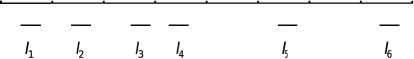
Figure 7.1. A sample of the ${\mathcal{I}}(N,M,\delta)$-pattern with $N=8$, $M=6$ and some positive $\delta$. The collection of the intervals ${\mathcal{I}}_{i}$, $1\leqslant i\leqslant 6$, forms the ${\mathcal{I}}(8,6,\delta)$-pattern.

We remark that for our setting the exponential sums have large values at the intervals ${\mathcal{I}}_{i}$, $1\leqslant i\leqslant 4$, of Figure 7.1. Moreover for each interval ${\mathcal{I}}_{i}$, $1\leqslant i\leqslant 4$, there are some subintervals which admits large exponential sums as well. Thus by the iterated construction the exponential sums have large values on a Cantor-like set, and therefore this gives the lower bounds of Theorem 2.6 and Theorem 2.7.

Remark 7.2.

We also use the notation ${\mathcal{J}}(N,M,\delta)$ when the above process is applied to the interval ${\mathcal{J}}$.

We construct Cantor sets by iterating the above ${\mathcal{I}}(N,M,\delta)$-patterns.

Let $(M_{k})$ and $(N_{k})$ be two sequence natural numbers with $1\leqslant M_{k}\leqslant N_{k}$ and $N_{k}\geqslant 2$ for all $k\in{\mathbb{N}}$. Let $(\delta_{k})$ be a sequence of positive numbers with $\delta_{0}=1$ and $\delta_{k}\leqslant\delta_{k-1}/N_{k}$ for all $k\in{\mathbb{N}}$.

We start from an interval ${\mathcal{I}}_{0}$ and take a ${\mathcal{I}}_{0}(N_{1},M_{1},\delta_{1})$-pattern inside of ${\mathcal{I}}_{0}$. Let ${\mathfrak{C}}_{1}$ be the collection of these $M_{1}$-subintervals. More precisely, let

$${\mathfrak{C}}_{1}=\{{\mathcal{I}}_{i}:\leavevmode\nobreak\ 1\leqslant i\leqslant M_{1}\}.$$

Note that each subinterval ${\mathcal{I}}_{i}$, $1\leqslant i\leqslant M_{1}$, has length $\delta_{1}$. For each ${\mathcal{I}}_{i}$ we take an ${\mathcal{I}}_{i}(N_{2},M_{2},\delta_{2})$-pattern inside of ${\mathcal{I}}_{i}$, and we denote these subintervals of ${\mathcal{I}}_{i}$ by ${\mathcal{I}}_{i,j}$ with $1\leqslant j\leqslant M_{2}$. Let

$${\mathfrak{C}}_{2}=\{{\mathcal{I}}_{i,j}:\leavevmode\nobreak\ 1\leqslant i\leqslant M_{1},\ 1\leqslant j\leqslant M_{2}\}.$$

Note that the choices of ${\mathcal{I}}_{i}(N_{2},M_{2},\delta_{2})$-pattern and ${\mathcal{I}}_{j}(N_{2},M_{2},\delta_{2})$-pattern are independent for $i\neq j$.

Suppose that we have ${\mathfrak{C}}_{k}$ which is a collection of

$$\#{\mathfrak{C}}_{k}=\prod_{i=1}^{k}M_{k}$$

intervals of length $\delta_{k}$. For each of these intervals ${\mathcal{I}}\in{\mathfrak{C}}_{k}$ we select a ${\mathcal{I}}(N_{k+1},M_{k+1},\delta_{k+1})$-pattern inside of ${\mathcal{I}}$. Let ${\mathfrak{C}}_{k+1}$ be the collection of these intervals, that is

$${\mathfrak{C}}_{k+1}=\{{\mathcal{I}}_{i_{1},\ldots,i_{k+1}}:\leavevmode\nobreak\ 1\leqslant i_{1}\leqslant M_{1},\ldots,1\leqslant i_{k+1}\leqslant M_{k+1}\}.$$

Our Cantor-like set is defined by

$${\mathcal{F}}=\bigcap_{k=1}^{\infty}{\mathcal{F}}_{k},$$

where

$${\mathcal{F}}_{k}=\bigcup_{{\mathcal{I}}\in{\mathfrak{C}}_{k}}{\mathcal{I}}.$$

There are uncountably many possible configurations for the above construction, we let $\Omega((N_{k}),(M_{k}),(\delta_{k}))$ denote the collections of all the possible configurations.

For determining the Hausdorff dimension of such a set, we use the following mass distribution principle, see [16, Theorem 4.2].

Lemma 7.3.

Let ${\mathcal{X}}\subseteq{\mathbb{R}}$ and let $\mu$ be a Borel measure on ${\mathbb{R}}$ such that

$$\mu({\mathcal{X}})>0.$$

If there exist $c$ and $\delta$ such that for any interval $B(r)$ of length $r$ with $0<r<\delta$ we have

$$\mu(B(r))\leqslant cr^{s},$$

then $\dim{\mathcal{X}}\geqslant s$.

We believe the following general result is of independent interest and may find some other applications.

Lemma 7.4.

Using the above notation, suppose that

$$M_{k}\geqslant cN_{k},\quad k\in{\mathbb{N}},$$

for some absolute constant $c>0$. Then for any set

$${\mathcal{F}}\in\Omega((N_{k}),(M_{k}),(\delta_{k}))$$

we have

$$\dim{\mathcal{F}}=\liminf_{k\rightarrow\infty}\frac{\log\prod_{i=1}^{k}M_{i}}{\log(1/\delta_{k})}.$$

Proof.

It is convenient to define

$$P_{k}=\prod_{i=1}^{k}M_{i}.$$

Let

$$s=\liminf_{k\rightarrow\infty}\frac{\log P_{k}}{\log(1/\delta_{k})}.$$

For any $\varepsilon>0$ there exists a subsequence $k_{n}$, $n\in{\mathbb{N}}$ such that

(7.1) $$P_{k_{n}}\leqslant\delta_{k_{n}}^{-s-\varepsilon}$$

for all large enough $n$.

Observe that for each $k_{n}$ the set ${\mathcal{F}}$ is covered by $P_{k_{n}}$ intervals and each of them has length $\delta_{k_{n}}$. Combining with (7.1) we have

$$\delta_{k_{n}}^{s+2\varepsilon}P_{k_{n}}\leqslant\delta_{k_{n}}^{\varepsilon}.$$

Thus the definition of Hausdorff dimension implies that $\dim{\mathcal{F}}\leqslant s+2\varepsilon$. By the arbitrary choice of $\varepsilon>0$ we obtain that $\dim{\mathcal{F}}\leqslant s$.

Now we use the mass distribution principle to obtain a lower bound for $\dim E$. Thus we first construct a measure on ${\mathcal{F}}$. For each $k$ let $\nu_{k}$ be a probability measure on $\mathsf{T}$ such that

$$\nu_{k}({\mathcal{I}})=\frac{1}{\#{\mathfrak{C}}_{k}}=P_{k}^{-1},\qquad\forall{\mathcal{I}}\in{\mathfrak{C}}_{k},$$

where ${\mathfrak{C}}_{k}$ is the corresponding collection of $\#{\mathfrak{C}}_{k}=P_{k}$ intervals as in the above. The measure $\nu_{k}$ weakly converges to a measure $\mu$, see [31, Chapter 1].

Let $0<t<s$ then for all large enough $k$ we have

(7.2) $$P_{k}\geqslant\delta_{k}^{-t}.$$

For any interval $B(r)$ with $0<r<1$ there exists $k\in{\mathbb{N}}$ such that

$$\delta_{k+1}<r\leqslant\delta_{k}.$$

Since the value $\delta_{k+1}$ maybe quite smaller than the value $\delta_{k}$, we do a case by case argument according to the value of $r$.

Case 1: Suppose that $\delta_{k}/N_{k+1}\leqslant r<\delta_{k}$. Since the interval $B(r)$ intersects at most $3rN_{k+1}/\delta_{k}$ disjoint intervals of equal length $\delta_{k}/N_{k+1}$, and inside each of these intervals there exists at most one interval of ${\mathfrak{C}}_{k+1}$, we obtain that

$$\nu_{k+1}(B(r))\ll\frac{rN_{k+1}}{\delta_{k}P_{k+1}}.$$

Applying the condition $M_{k}\geqslant cN_{k}$, the estimate (7.2) and the assumption $r<\delta_{k}$, we obtain

$$\nu_{k+1}(B(r))\ll\frac{r}{\delta_{k}P_{k}}\ll\frac{r}{\delta_{k}}\delta_{k}^{t}=r\delta_{k}^{t-1}\ll r^{t}.$$

Case 2: Suppose that $\delta_{k+1}\leqslant r\leqslant\delta_{k}/N_{k+1}$. Note that the interval $B(r)$ intersects at most two intervals with equal length $\delta_{k}/N_{k+1}$ and thus meets at most two intervals of ${\mathfrak{C}}_{k+1}$. Combining with (7.2) and the assumption $\delta_{k+1}\leqslant r$, we have

$$\nu_{k+1}(B(r))\leqslant\frac{2}{P_{k+1}}\ll\delta_{k+1}^{t}\leqslant r^{t}.$$

Putting Case 1 and Case 2 together, we conclude that

(7.3) $$\nu_{k+1}(B(r))\ll r^{t}.$$

Note that for $\delta_{k+1}\leqslant r<\delta_{k}$ we have

$$\mu(B(r))\leqslant\nu_{k+1}(B(3r)).$$

By (7.3) we obtain $\mu(B(r))\ll r^{t}$. Applying Lemma 7.3, we arrive at $\dim{\mathcal{F}}\geqslant t$. By the arbitrary choice of $t<s$ we obtain that $\dim{\mathcal{F}}\geqslant s$, which finishes the proof.     $\sqcap$$\sqcup$

We remark that the condition $M_{k}\geqslant cN_{k},k\in{\mathbb{N}}$ appears naturally in the proofs of Theorems 2.6 and 2.7. Moreover, the dimension formula of Lemma 7.4 may not hold in general without the condition $M_{k}\geqslant cN_{k}$, $k\in{\mathbb{N}}$. However, there are upper bounds and lower bounds for the general situation and more general constructions of Cantor-like sets, see [18] for more details.

We now formulate the following result which fits into our application immediately.

Corollary 7.5.

Using above notation, suppose that

$$M_{k}\geqslant cN_{k},\quad k\in{\mathbb{N}}$$

for some constant $c>0$, and $M_{k}$ tends to infinity rapidly such that

$$\lim_{k\rightarrow\infty}\frac{\log\prod_{i=1}^{k-1}M_{i}}{\log M_{k}}=0.$$

Then for any ${\mathcal{F}}\in\Omega((N_{k}),(M_{k}),(\delta_{k}))$ we have

$$\dim{\mathcal{F}}=\liminf_{k\rightarrow\infty}\frac{\log M_{k}}{\log(1/\delta_{k})}.$$

7.2. Proof of Theorem 2.6

Let $f$ satisfy the conditions of Theorem 2.6 and let ${\mathcal{F}}_{\mathbf{a},c}(f)$ denote the set of $x\in{\mathcal{I}}$ such that

$$\left|\sum_{1\leqslant n\leqslant N}a_{n}e(xf(n))\right|\geqslant cN^{1/2}\quad\text{for infinitely many $N\in{\mathbb{N}}$}.$$

We construct a Cantor set inside ${\mathcal{F}}_{\mathbf{a},c}(f)$ then apply results of Section 7.1 to obtain the desired lower bound of $\dim{\mathcal{F}}_{\mathbf{a},c}(f)$.

For the construction of the Cantor set, we start from an arbitrary interval ${\mathcal{I}}\subseteq{\mathbb{R}}$ and some large number $N$. Applying Lemma 6.4 to the interval ${\mathcal{I}}$ and the number $N$, we obtain a collection (taking $M_{1}$ instead of $K$) of

(7.4) $$M_{1}\gg N^{\gamma-1/2-\tau}|{\mathcal{I}}|$$

pairwise $N^{-\gamma+1/2+\tau}$-separated intervals ${\mathcal{I}}_{i}$, $1\leqslant i\leqslant M_{1}$, satisfying

$$|{\mathcal{I}}_{i}|=N^{-\gamma+1/2+\tau}$$

such that there exists some $x_{i}\in{\mathcal{I}}_{i}$ with

(7.5) $$\left|\sum_{\left\lfloor N/2\right\rfloor\leqslant n\leqslant N}a_{n}{\mathbf{\,e}}\left(x_{i}f(n)\right)\right|\gg N^{1/2}.$$

Note that for any complex numbers $a$ and $b$, by the triangle inequality, we have

$$\max\{|a|,|b|\}\geqslant\max\{|a-b|-|b|,|b|\}\geqslant|a-b|/2.$$

Hence, the inequality (7.5) implies

(7.6) $$\begin{split}\max_{Q\leqslant N}&\left|\sum_{n\leqslant Q}a_{n}{\mathbf{\,e}}\left(x_{i}f(n)\right)\right|\\ &\qquad\geqslant\max\left\{\left|\sum_{n\leqslant N}a_{n}{\mathbf{\,e}}\left(x_{i}f(n)\right)\right|,\left|\sum_{n\leqslant N/2}a_{n}{\mathbf{\,e}}\left(x_{i}f(n)\right)\right|\right\}\\ &\qquad\geqslant\frac{1}{2}\left|\sum_{N/2<n\leqslant N}a_{n}{\mathbf{\,e}}\left(x_{i}f(n)\right)\right|\gg N^{1/2}.\end{split}$$

Furthermore, since the intervals ${\mathcal{I}}_{i}$, $1\leqslant i\leqslant M_{1}$, are $N^{-\gamma+1/2+\tau}$-separated, that is

$$\text{Dist}({\mathcal{I}}_{i},{\mathcal{I}}_{j})\geqslant N^{-\gamma+1/2+\tau},\qquad 1\leqslant i<j\leqslant M_{1},$$

we obtain that

(7.7) $$|x_{i}-x_{j}|\geqslant N^{-\gamma+1/2+\tau},\qquad 1\leqslant i<j\leqslant M_{1}.$$

We now set

(7.8) $$N_{1}=\left\lceil N^{\gamma-1/2-\tau}\right\rceil+1$$

and divide the interval ${\mathcal{I}}$ into $N_{1}$ subintervals of equal length $N_{1}^{-1}$. Note that the choice of $N_{1}$ makes sure that the length of the subinterval is slightly smaller than $N^{-\gamma+1/2+\tau}$.

For each $1\leqslant i\leqslant M_{1}$, among the above $N_{1}$ subintervals there is an interval ${\mathcal{J}}_{i}$ containing $x_{i}$. Indeed if $x_{i}$ meets two of them then we choose one only. By (7.7) we conclude that ${\mathcal{J}}_{k}$ and ${\mathcal{J}}_{\ell}$ are separated for all $1\leqslant k<\ell\leqslant M_{1}$. In fact what we need in the following construction is that ${\mathcal{J}}_{k}\neq{\mathcal{J}}_{\ell}$ for $1\leqslant k<\ell\leqslant M_{1}$.

For each ${\mathcal{J}}_{i}$, the estimate (7.6) and Corollary 6.2 imply that there exists a subinterval $\widetilde{{\mathcal{J}}}_{i}\subseteq{\mathcal{J}}_{i}$ with length $\delta_{1}=N^{-\gamma-\tau}$ such that

$$\max_{Q\leqslant N}\left|\sum_{n=1}^{Q}a_{n}{\mathbf{\,e}}\left(xf(n)\right)\right|\gg N^{1/2},\qquad\forall x\in\widetilde{{\mathcal{J}}}_{i}.$$

Note that the collection of intervals $\widetilde{{\mathcal{J}}}_{i}$, $1\leqslant i\leqslant M_{1}$, forms a ${\mathcal{I}}(N_{1},M_{1},\delta_{1})$-pattern as in Definition 7.1.

Let

$${\mathfrak{C}}_{1}=\{\widetilde{{\mathcal{J}}}_{i}:\leavevmode\nobreak\ i=1,\ldots,M_{1}\}.$$

Moreover, by (7.4) and (7.8) we have $M_{1}\gg N_{1}$ where the implied constant depends on ${\mathcal{I}}$.

Let ${\mathcal{F}}_{1}$ be the union of intervals of ${\mathfrak{C}}_{1}$. The set ${\mathcal{F}}_{1}$ is the first step in the construction of the desired Cantor-like set, see Figure 7.2 for the case $M_{1}=3$.

Suppose we have constructed a sequence ${\mathfrak{C}}_{1},\ldots,{\mathfrak{C}}_{k}$ where ${\mathfrak{C}}_{k}$ is a union of disjoint intervals ${\mathcal{I}}_{i}$, $1\leqslant i\leqslant\#{\mathfrak{C}}_{k}$, of equal length $\delta_{k}$. We next construct a set ${\mathfrak{C}}_{k+1}$ which is a union of disjoint intervals of equal length $\delta_{k+1}$ for suitable $\delta_{k+1}$.

Let $L_{k}$ satisfy

(7.9) $$\delta_{k}\geqslant L_{k}^{-\gamma+2},$$

which is chosen so our parameters in the construction of ${\mathfrak{C}}_{k+1}$ satisfy the conditions of Lemma 6.4. For each interval ${\mathcal{J}}\in{\mathfrak{C}}_{k}$, we use a similar argument to the above construction of ${\mathfrak{C}}_{1}$. To be precise, let

$$N_{k+1}=\lceil\delta_{k}L_{k}^{\gamma-1/2-\tau}\rceil+1.$$

We divide the interval ${\mathcal{J}}$ into $N_{k+1}$ subintervals of equal length $\delta_{k}N_{k+1}^{-1}$. Note that the choice of $N_{k+1}$ make sure that the length of the subinterval is slightly smaller than $L_{k}^{-\gamma+1/2+\tau}$.

For the interval ${\mathcal{J}}$ and $L_{k}$, applying Lemma 6.4, we conclude that among these $N_{k+1}$ intervals, there are $M_{k+1}$ intervals ${\mathcal{J}}_{{\mathcal{I}},1},\ldots,{\mathcal{J}}_{{\mathcal{I}},M_{k+1}}$ of length $L_{k}^{-\gamma+1/2+\tau}$ such that for each $1\leqslant\ell\leqslant M_{k+1}$ there is a $x_{\ell}\in{\mathcal{J}}_{{\mathcal{I}},\ell}$ satisfying

$$\max_{Q\leqslant L_{k}}\left|\sum_{n=1}^{Q}a_{n}{\mathbf{\,e}}\left(x_{\ell}f(n)\right)\right|\gg L_{k}^{1/2}.$$

Furthermore,

$$N_{k+1}\geqslant M_{k+1}\gg L_{k}^{\gamma-1/2-\tau}\delta_{k}\gg N_{k+1}.$$

For each $x_{\ell}$, $1\leqslant\ell\leqslant M_{k+1}$, by Corollary 6.2 there exists a subinterval $\widetilde{{\mathcal{J}}_{{\mathcal{I}},\ell}}\subseteq{\mathcal{J}}_{{\mathcal{I}},\ell}$ such that

$$|\widetilde{{\mathcal{J}}_{{\mathcal{I}},\ell}}|=\delta_{k+1}=L_{k}^{-\gamma-\tau}$$

and

(7.10) $$\max_{Q\leqslant L_{k}}\left|\sum_{n=1}^{Q}a_{n}{\mathbf{\,e}}\left(xf(n)\right)\right|\gg L_{k}^{1/2},\qquad\forall x\in\widetilde{{\mathcal{J}}_{{\mathcal{I}},\ell}}.$$

Thus the collection of intervals $\widetilde{{\mathcal{J}}_{{\mathcal{I}},\ell}}$ forms a ${\mathcal{J}}(N_{k+1},M_{k+1},\delta_{k+1})$ pattern. Note that for ${\mathcal{J}}_{1},{\mathcal{J}}_{2}\in{\mathfrak{C}}_{k}$ with ${\mathcal{J}}_{1}\neq{\mathcal{J}}_{2}$ the two patterns ${\mathcal{J}}_{1}(N_{k+1},M_{k+1},\delta_{k+1})$ and ${\mathcal{J}}_{2}(N_{k+1},M_{k+1},\delta_{k+1})$ may be different in general.

Let ${\mathfrak{C}}_{k+1}$ be the collection of these ${\mathcal{J}}(N_{k+1},M_{k+1},\delta_{k+1})$ patterns with ${\mathcal{J}}\in{\mathfrak{C}}_{k}$. Our desired Cantor set is defined as

$${\mathcal{F}}=\bigcap_{k=1}^{\infty}{\mathcal{F}}_{k},$$

where

$${\mathcal{F}}_{k}=\bigcup_{{\mathcal{I}}\in{\mathfrak{C}}_{k}}{\mathcal{I}}.$$

Figure 7.2. Two steps construction of the Cantor-like set with $M_{1}=3$ and $M_{2}=4$.

Note that the set ${\mathcal{F}}$ is an element of $\Omega((N_{k}),(M_{k}),(\delta_{k}))$ as defined in Section 7.1. Now we are going to show that

(7.11) $${\mathcal{F}}\subseteq{\mathcal{F}}_{\mathbf{a},c}(f)$$

for some choices of parameters $N_{k}$, $M_{k}$ and $\delta_{k}$, where $k\in{\mathbb{N}}$.

Let $x\in{\mathcal{F}}$ then $x\in{\mathcal{F}}_{k}$ for all $k\in{\mathbb{N}}$. The estimate (7.10) implies that there exists $Q_{k}$ such that

$$L_{k}^{1/2}\ll Q_{k}\leqslant L_{k},$$

and

$$\left|\sum_{n=1}^{Q_{k}}a_{n}{\mathbf{\,e}}\left(xf(n)\right)\right|\gg|Q_{k}|^{1/2}.$$

For each $k$ we choose $L_{k}$ large enough such that

(7.12) $$Q_{1}<Q_{2}<\ldots,$$

which implies

$$\sum_{n=1}^{Q}a_{n}{\mathbf{\,e}}\left(xf(n)\right)\gg Q^{1/2}$$

for infinitely many $Q\in{\mathbb{N}}$ and hence we have (7.11). For each $k$ we can choose $L_{k}$ even larger such that the conditions (7.9), (7.12) hold, and

$$\lim_{n\rightarrow\infty}\frac{\log\prod_{i=1}^{n}N_{i}}{\log N_{n+1}}=0,$$

Clearly the condition $N_{k}\asymp M_{k}$, $k\in{\mathbb{N}}$ implies

$$\lim_{n\rightarrow\infty}\frac{\log\prod_{i=1}^{n}M_{i}}{\log M_{n+1}}=0.$$

Hence Corollary 7.5 applies and yields

$$\dim{\mathcal{F}}=\liminf_{k\rightarrow\infty}\frac{\log N_{k}}{\log(1/\delta_{k})}=\frac{\gamma-1/2-\tau}{\gamma+\tau},$$

and the result follows from (7.11) since $\tau>0$ is arbitrary.

7.3. Proof of Theorem 2.7

The proof is similar to the proof of Theorem 2.6, so we only give a sketch. Let $f$ satisfy the conditions of Theorem 2.7 and let ${\mathcal{F}}_{\mathbf{a},c}(f)$ denote the set of $x\in{\mathcal{I}}$ such that

$$\left|\sum_{n=1}^{N}a_{n}{\mathbf{\,e}}(xf(n))\right|\geqslant cN^{1/2}\quad\text{for infinitely many $N\in{\mathbb{N}}$}.$$

Similarly to the proof of Theorem 2.6, first of all we construct a Cantor set inside ${\mathcal{F}}_{\mathbf{a},c}(f)$.

Fix a small parameter $\tau>0$. Let $L\in{\mathbb{N}}$ be a large number and let

$$N_{1}=\left\lfloor\lambda({\mathcal{I}})L^{\gamma-1-\tau}\right\rfloor.$$

Divide ${\mathcal{I}}$ into $N_{1}$ subintervals of length $|{\mathcal{I}}|/N_{1}\gg L^{1-\gamma-\tau}$ which we denote as ${\mathcal{I}}_{1},\ldots,{\mathcal{I}}_{N_{1}}$.

Applying Lemma 4.1 to each interval ${\mathcal{I}}_{k},1\leqslant k\leqslant N_{1}$, there exists $x_{k}\in{\mathcal{I}}_{k}$ such that

$$\left|\sum_{n=L}^{2L}a_{n}{\mathbf{\,e}}\left(x_{k}f(n)\right)\right|\gg L^{1/2}.$$

Applying similar arguments to the proof of (7.6), we obtain

$$\max_{Q\leqslant 2L}\left|\sum_{n=1}^{Q}a_{n}{\mathbf{\,e}}(x_{k}f(n))\right|\gg L^{1/2}.$$

For each $x_{k}$, applying Corollary 6.2 and using that $f(t)\leqslant t^{\gamma+o(1)}$, we obtain that there exists an interval ${\mathcal{J}}_{k}\subseteq{\mathcal{I}}_{k}$ with length $|{\mathcal{J}}_{k}|=L^{-\gamma-\tau}$ such that

$$\max_{Q\leqslant 2L}\left|\sum_{n=1}^{Q}a_{n}{\mathbf{\,e}}(xf(n))\right|\gg L^{1/2},\qquad\forall x\in{\mathcal{J}}_{k}.$$

Note that the collection of intervals ${\mathcal{J}}_{k}\subseteq{\mathcal{I}}_{k}$, $1\leqslant k\leqslant N_{1}$, forms an ${\mathcal{I}}(N_{1},N_{1},L^{-\gamma-\tau})$-pattern as in Definition 7.1. Furthermore, this is the first step of the construction of the desired Cantor-like set, and we denote the union of these intervals ${\mathcal{J}}_{k},1\leqslant k\leqslant N_{1}$, as ${\mathcal{C}}_{1}$.

Let $L_{k},k\in{\mathbb{N}}$ be a rapidly increasing sequence of numbers, for instance

(7.13) $$\log L_{k+1}\geqslant L_{1}L_{2}\ldots L_{k}.$$

Suppose that we have constructed $k$-level Cantor set ${\mathcal{C}}_{k}$ which is a collection of disjoint intervals with equal length $\delta_{k}$. Let $N_{k+1}=\left\lfloor\delta_{k}L_{k+1}^{\gamma-1-\tau}\right\rfloor$ and for each ${\mathcal{J}}\in{\mathcal{C}}_{k}$ we divide the interval ${\mathcal{J}}\in{\mathcal{C}}_{k}$ into $N_{k+1}$ subintervals of length

$$|{\mathcal{J}}|/N_{k+1}\gg L_{k+1}^{1-\gamma+\tau}.$$

Applying the same argument as above to the interval ${\mathcal{J}}$, there exists a ${\mathcal{J}}(N_{k+1},N_{k+1},\delta_{k+1})$-pattern ${\mathcal{A}}\subseteq{\mathcal{J}}$ such that

(7.14) $$\delta_{k+1}=L_{k+1}^{-\gamma-\tau},$$

and

$$\max_{Q\leqslant 2L_{k+1}}\left|\sum_{n=1}^{Q}a_{n}{\mathbf{\,e}}\left(xf(n)\right)\right|\gg Q^{1/2},\qquad\forall\ x\in{\mathcal{A}}.$$

Let ${\mathcal{C}}_{k+1}$ be a collection of the ${\mathcal{J}}(N_{k+1},N_{k+1},\delta_{k+1})$-patterns inside each interval ${\mathcal{J}}\in{\mathcal{C}}_{k}$, see Remark 7.2. The desired Cantor set is defined as

$${\mathcal{C}}=\bigcap_{k=1}^{\infty}{\mathcal{C}}_{k}.$$

Note that for some small constant $c>0$ the Cantor-like set ${\mathcal{C}}$ is subset of ${\mathcal{F}}_{\mathbf{a},c}(f)$.

By (7.13) and (7.14) we conclude that for each $k\in{\mathbb{N}}$ the set ${\mathcal{C}}_{k+1}$ contains

$$\prod_{i=1}^{k+1}N_{i}=L_{k+1}^{\gamma-1-\tau+o(1)}$$

intervals with equal length

$$\delta_{k+1}=L_{k+1}^{-\gamma-\tau}.$$

Combining with Corollary 7.5 and the arbitrary choice of $\tau>0$ we conclude that

$$\dim{\mathcal{C}}\geqslant 1-1/\gamma,$$

which finishes the proof.

8. Some heuristics on the Hausdorff dimension of the sets of large sums

We start with the case of monomial sums. In particular, recall the notation (1.4) and (1.5). It is natural to assume that $\sigma_{d}(x;N)$ is large only if $x$ can be well approximated by a rational number with a reasonably small denominator, that is, belongs to major arcs in the traditional terminology, see [37]. While qualitatively this is an established fact, its optimal quantitive version is still unclear. Here we base our heuristics on an approximate formula of Vaughan [37, Theorem 4.1]. More precisely, if

$$x=\frac{a}{q}+\xi$$

for some integers $a$ and $q\geqslant 1$ with $\gcd(a,q)=1$ then

(8.1) $$\begin{split}\sigma_{d}(x;N)=\frac{1}{q}\sigma_{d}(a/q;q)&\int_{0}^{N}{\mathbf{\,e}}\left(\xi\gamma^{d}\right)d\gamma\\ &\qquad+O\left(q^{1/2+o(1)}\left(1+|\xi|N^{d}\right)^{1/2}\right).\end{split}$$

It is also shown in [8] that the error term is close to optimal. First we observe that if $\xi<0.5N^{-d}$ then

$$\left|\int_{0}^{N}{\mathbf{\,e}}\left(\xi\gamma^{d}\right)d\gamma\right|\gg N.$$

Now assuming that “typically” we have $\sigma_{d}(a/q;q)=q^{1/2+o(1)}$, we conclude that

$$\left|\sigma_{d}(x;N)\right|\geqslant Nq^{-1/2+o(1)}+O\left(q^{1/2+o(1)}\right).$$

For any $\alpha>1/2,$ setting $N=\left\lfloor q^{1/2(1-\alpha)+\varepsilon}\right\rfloor$ we obtain that for any $x\in\mathsf{T}$ such that

(8.2) $$\left|x-\frac{a}{q}\right|<q^{-d/2(1-\alpha)-d\varepsilon}$$

holds for infinitely many $a$ and $q\geqslant 1$ with $\gcd(a,q)=1$, we have

$$\left|\sigma_{d}(x;N)\right|\geqslant N^{\alpha}$$

for infinitely many $N$. The argument in the proof of the classical Jarník–Besicovitch theorem, see [16, Theorem 10.3], implies that the set of $x\in\mathsf{T}$ satisfying $|x-a/q|\leqslant q^{-\kappa}$ for infinitely many irreducible fractions $a/q$ with some fixed $\kappa\geqslant 2$, is of Hausdorff dimension $2/\kappa$. Hence, recalling (8.2), it seems reasonably to conjecture that

$$\dim\mathscr{F}_{d,\alpha}=\frac{4(1-\alpha)}{d}.$$

In particular, compared with (1.6), for $d\geqslant 3$ this suggests that there is a discontinuity in the behaviour of $\dim\mathscr{F}_{d,\alpha}$ as a function of $\alpha$, most likely at $\alpha=1/2$.

In principle similar arguments also apply to $\mathscr{E}_{d,\alpha}$ and may also lead to a conjecture about $\dim\mathscr{E}_{d,\alpha}$. Instead of (8.1), we now recall a result of Baker [1, Lemma 4.4] which asserts that if for $\mathbf{x}\in\mathsf{T}_{d}$ we have

(8.3) $$x_{i}-\frac{a_{i}}{q}=\xi_{i}$$

with some integers $a_{1},\ldots,a_{d}$ and $q\geqslant 1$ and real numbers

(8.4) $$|\xi_{i}|\leqslant\frac{1}{2d^{2}qN^{i-1}},\qquad i=1,\ldots d,$$

then

(8.5) $$\begin{split}S_{d}(\mathbf{x};N)&=\frac{1}{q}S_{d}(\mathbf{a}/q;q)\int_{0}^{N}{\mathbf{\,e}}\left(\xi_{d}\gamma^{d}+\ldots+\xi_{1}\gamma\right)d\gamma\\ &\qquad\qquad\qquad\qquad\qquad\quad+O\left(q^{1-1/d+o(1)}D^{1/d}\right),\end{split}$$

where

$$\mathbf{a}=(a_{1},\ldots,a_{d})\qquad\mbox{and}\qquad D=\gcd(a_{2},\ldots,a_{d},q).$$

We now assume that for all but a negligible set of $\mathbf{x}\in\mathsf{T}_{d}$ (say, of Hausdorff dimension zero) the following holds:

• the corresponding exponential sums have square root cancellation, which holds, if for example the denominators $q$ are essentially square-free up to a factor of size $q^{o(1)}$;

• we have $D=q^{o(1)}$.

These are the main heuristic assumptions of our approach. Under these assumptions, analysing the proof of (8.5) in [1], we see that (8.5) can heuristically be transformed into

(8.6) $$\begin{split}S_{d}(\mathbf{x};N)&=\frac{1}{q}S_{d}(\mathbf{a}/q;q)\int_{0}^{N}{\mathbf{\,e}}\left(\xi_{d}\gamma^{d}+\ldots+\xi_{1}\gamma\right)d\gamma\\ &\qquad\qquad\qquad\qquad\qquad\qquad\qquad+O\left(q^{1/2+o(1)}\right).\end{split}$$

Furthermore, if

$$|\xi_{i}|\leqslant\frac{1}{2d^{2}N^{i}},\qquad i=1,\ldots d,$$

then

$$\left|\int_{0}^{N}{\mathbf{\,e}}\left(\xi\gamma^{d}\right)d\gamma\right|\gg N,$$

and thus

$$\left|S_{d}(\mathbf{x};N)\right|\geqslant Nq^{-1/2+o(1)}+O\left(q^{1/2+o(1)}\right),$$

provided that

$$\left|x_{i}-\frac{a}{q}\right|<\frac{1}{2d^{2}N^{i}}\leqslant\frac{1}{2d^{2}qN^{i-1}},\qquad i=1,\ldots d,$$

(ignoring a very small set of $\mathbf{x}\in\mathsf{T}_{d}$).

For any $1/2<\alpha<1$, setting $N=\left\lfloor q^{1/2(1-\alpha)+\varepsilon}\right\rfloor$, we obtain that for any $\mathbf{x}\in\mathsf{T}_{d}$ such that there are infinitely many approximations

$$\left|x_{i}-\frac{a_{i}}{q}\right|<q^{-i/2(1-\alpha)-i\varepsilon},\qquad i=1,\ldots d,$$

we have $|S_{d}(\mathbf{x};N)|\geqslant N^{\alpha}$ for infinitely many $N$.

Let ${\mathcal{X}}_{d,\alpha}$ be the set of $\mathbf{x}\in\mathsf{T}_{d}$ such that there are infinitely many approximations

$$\left|x_{i}-\frac{a_{i}}{q}\right|<q^{-i/2(1-\alpha)},\qquad i=1,\ldots d.$$

This naturally leads us to the conjecture that

$$\dim\mathscr{E}_{d,\alpha}=\dim{\mathcal{X}}_{d,\alpha}.$$

We also consider the set ${\mathcal{X}}_{d,\alpha}^{\sharp}\subseteq{\mathcal{X}}_{d,\alpha}$, which is defined exactly as ${\mathcal{X}}_{d,\alpha}$ with the additional condition that the denominator $q=p$ is prime. That is, ${\mathcal{X}}_{d,\alpha}^{\sharp}$ is the set of $\mathbf{x}\in\mathsf{T}_{d}$ such that there are infinitely many approximations

$$\left|x_{i}-\frac{a_{i}}{p}\right|<p^{-i/2(1-\alpha)},\qquad i=1,\ldots d,$$

with a prime $p$.

We also note that for $\mathbf{x}\in\mathsf{T}_{d}$ such that with a prime $q=p$ we have (8.3) and (8.4), using the Weil bound, see, for example, [30, Chapter 6, Theorem 3], in the argument of the proof of [1, Lemma 4.4], the asymptotic formula (8.6) can be established rigorously with $p$ instead of $q$.

We also recall that by a result of Knizhnerman and Sokolinskii [28, Theorem 1], see also [29], there is positive proportion of rational exponential sums $S_{d}(\mathbf{a}/p;p)$, which are of order $p^{1/2}$, that is, with

(8.7) $$\left|S_{d}(\mathbf{a}/p;p)\right|\gg p^{1/2}.$$

Furthermore, by [10, Lemma 2.6], the corresponding coefficients $\mathbf{a}/p=(a_{1}/p,\ldots,a_{d}/p)$ are densely distributed in the cube $[0,1]^{d}$. This shows that the main term in (8.6) is large for a large subset of $\mathbf{x}\in\mathsf{T}_{d}$. We remark that for $d=2$, that is, for Gauss sums, the bound (8.7) holds for all $(a_{1}/p,a_{2}/p)$ with $a_{2}\neq 0$, see [27, Equation (1.55)].

Hence, using the above observations, one can perhaps produce a rigorous argument that

$$\dim\mathscr{E}_{d,\alpha}\geqslant\dim{\mathcal{X}}_{d,\alpha}^{\sharp}.$$

Applying a result of Rynne [34, Theorem 1] we obtain

$$\dim{\mathcal{X}}_{d,\alpha}^{\sharp}=\dim{\mathcal{X}}_{d,\alpha}=\mathfrak{s}(d,\alpha),$$

where

$$\mathfrak{s}(d,\alpha)=\min_{j=1,\ldots,d}\frac{d+1+j\vartheta_{j}-\sum_{i=1}^{j}\vartheta_{i}}{1+\vartheta_{j}},$$

and

$$\vartheta_{i}=\frac{i}{2(1-\alpha)}-1,\qquad i=1,\ldots,d.$$

We remark that the condition $\alpha\geqslant 1/2$ makes sure the assumption of [34, Theorem 1] holds, that is, we have

$$\sum_{i=1}^{d}\vartheta_{i}\geqslant 1.$$

For a different approach to $\dim{\mathcal{X}}_{d,\alpha}^{\#}$ and $\dim{\mathcal{X}}_{d,\alpha}$, see also [38, Corollary 5.1].

We recall that the upper bound of $\dim\mathscr{E}_{d,\alpha}$ in [11, Theorem 1] claims that for $d\geqslant 2$ and $\alpha\in(1/2,1)$ one has

$$\dim\mathscr{E}_{d,\alpha}\leqslant\mathfrak{u}(d,\alpha),$$

where

$$\mathfrak{u}(d,\alpha)=\min_{k=0,\ldots,d-1}\frac{(2d^{2}+4d)(1-\alpha)+k(k+1)}{4-2\alpha+2k}.$$

We now compare the values of $\mathfrak{s}(d,\alpha)$ and $\mathfrak{u}(d,\alpha)$ for $d=2$. We have

$$\mathfrak{s}(2,\alpha)=\begin{cases}\displaystyle\frac{7-6\alpha}{2}&\text{for }1/2\leqslant\alpha\leqslant 5/6,\\ 6(1-\alpha)&\text{for }5/6<\alpha<1,\end{cases}$$

and

$$\mathfrak{u}(2,\alpha)=\begin{cases}\displaystyle\frac{9-8\alpha}{3-\alpha}&\text{for }1/2\leqslant\alpha\leqslant 6/7,\\ \displaystyle\frac{8(1-\alpha)}{2-\alpha}&\text{for }6/7<\alpha<1.\end{cases}$$

Note that for the endpoints $\alpha=1/2$ and $\alpha=1$ we have

$$\mathfrak{s}(2,1/2)=\mathfrak{u}(2,1/2)=2,$$

and

$$\mathfrak{s}(2,1)=\mathfrak{u}(2,1)=0.$$

Moreover, it is somewhat tedious but elementary to derive that

$$\mathfrak{s}(2,\alpha)<\mathfrak{u}(2,\alpha),\qquad 1/2<\alpha<1.$$

For the case $d\geqslant 3$ and for the value $\mathfrak{u}(d,\alpha)$ we have

$$\mathfrak{u}(d,1/2)=d\qquad\mbox{and}\qquad\mathfrak{u}(d,1)=0.$$

However, for the value $\mathfrak{s}(d,1/2)$ we have

$$\mathfrak{s}(d,1/2)=\min_{j=1,\ldots,d}\frac{2(d+1)+j^{2}-j}{2j}.$$

Thus we have

$$\lim_{d\to\infty}\mathfrak{s}(d,1/2)/\sqrt{2d}=1.$$

In particular, compared with (1.6) this suggests that, as in the case of $\dim\mathscr{F}_{d,\alpha}$, there is a discontinuity in the behaviour of $\dim\mathscr{E}_{d,\alpha}$, most likely at $\alpha=1/2$ when $d\geqslant 3$.

References

- [1] R. C. Baker, Diophnatine inequalities, Oxford Univ. Press, 1986.
- [2] E. Bombieri, ‘On exponential sums in finite fields’, Amer. J. Math., 88 (1966), 71–105.
- [3] J. Bourgain, C. Demeter and L. Guth, ‘Proof of the main conjecture in Vinogradov’s mean value theorem for degrees higher than three’, Ann. Math., 184 (2016), 633–682.
- [4] T. D. Browning, ‘Equal sums of two th powers’, J. Number Theory, 96 (2002), 293–318.
- [5] T. D. Browning, ‘Sums of four biquadrates’, Math. Proc. Cambridge Philos. Soc., 134 (2003), 385–395.
- [6] T. D. Browning and D. R. Heath-Brown, ’Plane curves in boxes and equal sums of two powers’, Math. Zeit., 251 (2005), 233–247.
- [7] J. Brüdern, ‘Approximations to Weyl sums’, Acta Arith., 184 (2018), 287–296.
- [8] J. Brüdern and D. Daemen, ‘Imperfect mimesis of Weyl sums’, Internat. Math. Res. Notices,, 2009 (2009), 3112–3126.
- [9] J. W. S. Cassels ‘Some metrical theorems in Diophantine approximation. I’, Proc. Cambridge Philos. Soc., 46 (1950), 209–218.
- [10] C. Chen and I. E. Shparlinski, ‘On large values of Weyl sums’, Adv. Math., 370 (2020). Article 107216.
- [11] C. Chen and I. E. Shparlinski, ‘Hausdorff dimension of the large values of Weyl sums’, J. Number Theory, 214 (2020) 27–37.
- [12] C. Chen and I. E. Shparlinski, ‘New bounds of Weyl sums’, Intern. Math. Res. Notices, (to appear).
- [13] J. Cilleruelo and A. Granville, ‘Lattice points on circles, squares in arithmetic progressions, and sumsets of squares’, Additive Combinatorics, CRM Proceedings Lecture Notes, 43 (2007), 241–262.
- [14] M. Drmota and R. Tichy, Sequences, discrepancies and applications, Springer-Verlag, Berlin, 1997.
- [15] L. C. Evans and R. F. Gariepy, Measure theory and fine properties of functions. Boca Raton, FL, CRC, 1992.
- [16] K. J. Falconer, Fractal geometry: Mathematical foundations and applications, John Wiley, 2nd Ed., 2003.
- [17] A. Fedotov and F. Klopp, ‘An exact renormalization formula for Gaussian exponential sums and applications’, Amer. J. Math., 134 (2012), 711–748.
- [18] D. J. Feng, Z. Y. Wen and J. Wu, ‘Some dimensional results for homogeneous Moran sets’, Sci. China Ser. A., 40 (1997), 475–482.
- [19] H. Fiedler, W. Jurkat and O. Körner, ‘Asymptotic expansions of finite theta series’, Acta Arith., 32 (1977), 129–146.
- [20] P. Gallagher, ‘Approximation by reduced fractions’, J. Math. Soc. Japan, 13, (1961), 342–345.
- [21] G. H. Hardy and J. E. Littlewood, ‘The trigonometric series associated with the elliptic -functions’, Acta Math., 37 (1914), 193–239.
- [22] G. H. Hardy and J. E. Littlewood, ‘Some problems of Diophantine approximation: A remarkable trigonometric series’, Proc. Nat. Acad. Sci., 2 (1916), 583–586.
- [23] D. R. Heath-Brown, ‘The density of rational points on cubic surfaces’, Acta Arith., 79 (1997), 17–30.
- [24] D. R. Heath-Brown, ’Counting rational points on algebraic varieties’, Analytic number theory, Lecture Notes in Math., vol. 1891, Springer, Berlin, 2006, 51–95,
- [25] C. Hooley, ‘On another sieve method and the numbers that are a sum of two th powers’, Proc. London Math. Soc., 36 (1978), 117–140.
- [26] C. Hooley, ‘On another sieve method and the numbers that are a sum of two th powers, II’, J. Reine Angew Math., 475 (1996), 55–75.
- [27] H. Iwaniec and E. Kowalski, Analytic number theory, Amer. Math. Soc., Providence, RI, 2004.
- [28] L. A. Knizhnerman and V. Z. Sokolinskii, ‘Some estimates for rational trigonometric sums and sums of Legendre symbols’, Uspekhi Mat. Nauk, 34 (3) (1979), 199–200 (in Russian); translated in Russian Math. Surveys, 34 (3) (1979), 203–204.
- [29] L. A. Knizhnerman and V. Z. Sokolinskii, ‘Trigonometric sums and sums of Legendre symbols with large and small absolute values’, Investigations in Number Theory, Saratov, Gos. Univ., Saratov, 1987, 76–89 (in Russian).
- [30] W.-C. W. Li, Number theory with applications, World Scientific, Singapore, 1996.
- [31] P. Mattila, Geometry of sets and measures in Euclidean spaces: Fractals and rectifiability, Cambridge Univ. Press, 1995.
- [32] O. Mormon, ‘Sums and differences of four th powers’, Monat. Math., 164 (2011), 55–74.
- [33] W. Rudin, ‘Some theorems on Fourier coefficients’, Proc. Amer Math. Soc., 10 (1959), 855–859.
- [34] B. P. Rynne, ‘Hausdorff dimension and generalized simultaneous Diophantine approximation’, Bull. London Math. Soc. 30 (1998), 365–376.
- [35] C. M. Skinner and T. D. Wooley, ’Sums of two th powers’, J. Reine Angew Math., 462 (1995), 57–68.
- [36] S. A. Stepanov, ‘Rational trigonometric sums along a curve’, Automorphic Functions and Number Theory, II, Zap. Nauchn. Sem. Leningrad. Otdel. Mat. Inst. Steklov., vol. 134 (1984), 232–251 (in Russian).
- [37] R. C. Vaughan, The Hardy-Littlewood method, Cambridge Tracts in Math. vol. 25, Cambridge Univ. Press, 1997.
- [38] B. Wang, J. Wu and J. Xu, ‘Mass transference principle for limsup sets generated by rectangles’. Math. Proc. Cambridge Philos. Soc., 158 (2015), 419–437.
- [39] T. D. Wooley, ‘The cubic case of the main conjecture in Vinogradov’s mean value theorem’, Adv. in Math., 294 (2016), 532–561.
- [40] T. D. Wooley, ‘Perturbations of Weyl sums’, Internat. Math. Res. Notices, 2016 (2016), 2632–2646.
- [41] T. D. Wooley, ‘Nested efficient congruencing and relatives of Vinogradov’s mean value theorem’, Proc. London Math. Soc., 118 (2019), 942–1016.