Stable Bounded Excursion Gravastars with Regular Black Holes

Abstract

This paper explores the possible existence of stable regions of bounded excursion gravastars in the background of regular black holes (Bardeen and Bardeen-de Sitter black holes). For this purpose, we match internal de Sitter geometry with an external regular black hole through an intermediate shell with an equation of state. The matter surface located at the shell greatly affects the dynamical configuration of the shell. We consider stiff and dust fluids to discuss the outcomes of the developed structures. We then determine the critical values of physical parameters at which the shell neither collapses nor expands for both cases with different choices of external and internal geometries. It is found that there does not exist any possible region of stable bounded excursion gravastar for the interior flat and exterior regular geometries. However, the stable bounded excursion gravastar is obtained for the interior de Sitter and exterior regular black holes with a suitable choice of physical parameters for both stiff and dust shells. We conclude that the possibility of the existence of both bounded excursion gravastars as well as black holes cannot be excluded in the dynamical model.

Keywords: Gravastars; Israel formalism; Stability analysis.
PACS: 04.70.Dy; 97.10.Cv; 04.40.Nr; 04.40.Dg

1 Introduction

The gravitational collapse has been one of the interesting research fields which lead to the formation of different compact objects such as white dwarfs, neutron stars, naked singularities, and black holes (BHs). In the light of theoretical and observational advances, there is often a set of paradoxical issues surrounding the BHs that inspires scholars to try other solutions where massive stars are without horizons at their endpoints of gravitational collapse (Wald 2001). Gravastars (Mazur and Mottola 2001; 2004), Bose superfluid (Chapline et al 2003) and black stars are a few examples of such physical models. Within such simulations, gravastars have obtained a particular interest in recent times, in part, owing to the strong relationship between the cosmological constant and the expanding universe (Copeland et al 2006), even though the presence of these stars may be limited very narrowly on observational grounds. A gravastar (gravitation expectation star) is an astronomic object proposed as an alternative to BH with no event horizon and singularity.

Mazur and Mottola (2004) considered the Visser cut and paste approach to develop a gravastar model from the joining of exterior Schwarzschild BH with interior de Sitter (dS) spacetime. This model can be described in three different regions with the specific equation of state (EoS). The first region is denoted as an interior ($0\leq r<r_{1}$), second is the intermediate ($r_{1}<r<r_{2}$) and third is referred to as an exterior region ($r_{2}<r$). In the first zone, a repulsive force is generated in the intermediate region by the isotropic pressure ($p=-\sigma$, where $\sigma$ is the energy density). The intermediate region is assumed to be shielded by ultra-relativistic plasma and fluid pressure ($p=\sigma$). The exterior region is supported by the vacuum solution of the field equations with zero pressure ($p=0=\sigma$). This provides an effective thermodynamic solution with small fluctuations and maximum entropy.

The thin-shell matter surface produces an adequate amount of pressure to counteract the strength of gravity effects that maintain its configuration stable. Visser and Wiltshire (2004) found the simplest model to represent the Mazur-Mottola scenario by combining external and internal geometries using the cut and paste method. They evaluated the stable structure of gravastar with a suitable choice of EoS for the transition layers. There are two different approaches to studying the dynamics and stability of thin-shell. The first is to prescribe a potential $V(a)$ and leave the EoS of the shell as derived. The second is to prescribe an EoS of the shell and leave the potential $V(a)$ as derived. They followed the first approach and studied in detail the case where $V(a_{0})=0$, $V^{\prime}(a_{0})=0$ and $V^{\prime\prime}(a_{0})>0$. Here, prime denotes the ordinary derivative to the indicated argument. The developed structure is said to be stable if there exists shell radius $a_{0}$ for which the above conditions are verified. There is a less stringent notion of stability known as bounded excursion models, in which there exist two radii $a_{1}$ and $a_{2}$ with ($a_{1}<a_{2}$) such that $V(a_{1})=0$, $V^{\prime}(a_{1})<0$ and $V(a_{2})=0$, $V^{\prime}(a_{2})>0$. Carter (2005) extended this concept by the joining of interior dS spacetime and exterior Reissner-Nordström (RN) BH. Horvat et al. (2009) introduced a theoretical electromagnetic gravastar model and investigated the effects of charge on stable gravastar configuration. The physical features such as entropy, proper length, and energy content of charged gravastar in (2+1)-dimensional spacetime were analyzed by Rahaman et al. (2012a; 2012b).

Timelike thin-shells in spherically symmetric static spacetimes are the most interesting cosmological objects which can be constructed in general relativity. Such models of cosmological objects have been used to analyze some astrophysical phenomena such as gravitational collapse and supernova explosions. The seminal work of Israel (1966; 1967) provided a concrete formalism for constructing timelike shells, in general, by gluing two different manifolds at the location of the thin-shell. Self-gravitating thin-shells are the solutions of a given gravitational theory describing two regions separated by an infinitesimally thin region where the matter is confined. It is important to determine whether relevant thin-shell configurations are stable, both thermodynamically and dynamically.

Many researchers have discussed the dynamics and stable configuration of thin-shell and thin-shell wormholes (WHs) by using radial perturbation with different matter distributions. Brady et al. (1991) investigated linear stability of thin-shell that connects inner flat and outer Schwarzschild BH through radial perturbation. Martinez (1996) studied thermodynamical stability of such a geometrical structure. Later, Mazharimousavi et al. (2017) explored stable configuration of such systems by using variable equation of state (EoS). LeMaitre and Poisson (2019) observed stability of this geometrical structure in Newtonian and relativistic gravity. They found a link between the existence of a maximum mass along a sequence of equilibrium configurations and the onset of dynamical instability. Recently, Bergliaffa et al. (2006) examined their linear and thermodynamical stability by considering barotropic and also for EoS of the type $p=p(\rho(a))$.

A requirement for a traversable WH is that the throat needs to be held open and lined with a stress-energy density that violates the energy conditions of general relativity. The source of such stress-energy tensor is often called exotic matter. To simplify the calculations and investigations of the stability of traversable WHs, Visser (1989) introduced a cut and paste method where the throat is cut out and the two mouths are pasted together. In this procedure, the exotic matter reduces in an infinitesimally thin-shell which connects two equivalent copies of BH spacetimes. For instance, the components of stress-energy tensor of thin-shell WHs allows us to conjure up different EoS and also study how these affect the WH stability. There is a large body of literature that explore the stable characteristics of thin-shell WHs in the background various singular and non-singular BH geometries (Halilsoya et al 2014; Lobo et al 2004; Eiroa and Simeone 2007; Mazharimousavi et al 2010; Dias and Lemos 2010; Amirabi et al 2013).

Rocha and his collaborators (2008a; 2008b) presented the prototype gravastar model by using external Schwarzschild BH and internal dS spacetime. They found that models sometimes represent stable bounded excursion gravastars, in which thin-shell oscillates between two final radii, otherwise, they collapse until BHs are formed. Hence, the possibility of the existence of a gravastar model cannot be excluded in such dynamical models. Chan et al. (2009a) proposed a dynamical model of prototype gravastars filled with phantom energy. It is found that the developed structure can be a BH, stable, unstable, or bounded excursion gravastar for various matter distributions at thin-shell. Later, this work was extended for the choice of exterior Schwarzschild-dS and RN spacetimes with interior dS region with specific EoS. They found that stable bounded excursion gravastar is obtained in the presence of exterior cosmological constant and charge (Chan et al 2009b; 2010).

Lobo and Arellano (2007) studied the gravstar models with non-linear electrodynamics. G$\acute{a}$sp$\acute{a}$r and R$\acute{a}$cz (2010) observed the stability of gravastars through the inelastic collision of their surface layer with a dust shell. Horvat et al. (2011) considered the gravastar with continuous pressure and examined stability through the conventional Chandrasekhar approach. Lobo and Garattini (2013) studied the stability of noncommutative thin-shell gravastar and found that stable regions must be located near the predicted location of the event horizon. Övgün et al. (2017) developed the gravastar model from the matching of external charged noncommutative BH with internal dS manifold. They noticed that the established framework satisfies the null energy condition and displays stable behavior for certain acceptable values of the physical parameter close to the predicted horizon.

Banerjee et al. (2018) developed thin-shell gravastar solutions with interior dS and exterior RN BH for a certain range of parameters where the metric potentials and electromagnetic fields are related in some particular relation called Guilfoyles solution. They also observed energy conditions and linearized stability of the developed structure. In the backgrounds of Bardeen/Bardeen-dS BHs, we have examined the stable regions of thin-shell gravastars through radial perturbation (Sharif and Javed 2020). It is found that stable regions decrease for large values of charge and increase for higher values of the cosmological constant. There is a large body of literature (Lobo 2006; DeBenedictis et al 2006; Horvat and Iliji$\acute{c}$ 2007; Chan et al 2011a; Horvat et al 2011; Chan et al 2011b; Banerjee and Rahaman 2016; Ghosh and Rahaman 2017; Shamir and Ahmad 2018; Yousaf et al 2019; Sharif and Waseem 2019; Bhattiet al 2020; Das 2020; Yousaf 2020) that explores the configuration thin-shell gravastars in the context of different scenarios.

The establishment of general relativity by Einstein was a great success of physics in the last century. However, there still remain a few difficulties out of which the existence of singularity is an intrinsic problem of general relativity. Regular black hole (BH) is a concept produced out of multiple attempts to establish an understandable interior structure for BH by avoiding singularity inside it. The study of BHs without singularities can help us to understand the role played by singularities in astrophysics. The study on global regularity of BHs has attained remarkable importance to understand the final state of initially regular configurations. None of the regular BHs are exact solutions to the Einstein field equations without any physically reasonable source.

The above-mentioned stable/unstable bounded excursion gravastar models are constructed in the background of exterior geometries with singularities. For the regular BHs (BHs without singularity), such geometrical structures have not been explored so far. Regular BHs are more interesting compact objects due to their regular center. Bardeen obtained a BH solution without singularity well-known as Bardeen BH (Bardeen 1968). Bardeen regular BHs are charged spacetimes which behave as ordinary RN BH solutions and the existence of these solutions does not contradict with the singularity theorems. Afterward, some more models of regular BHs were proposed (Ay$\acute{o}$n-Beato and Garc$\acute{i}$a (ABG) 1998; Bronnikov 2000; Hayward (2006)). Ay$\acute{o}$n-Beato and Garc$\acute{i}$a (2000) also proved that the Bardeen BH can be interpreted as a gravitationally collapsed magnetic monopole arising in a specific form of nonlinear electrodynamics. Hence, the stress-energy tensor of the nonlinear electrodynamics is considered as the source for the Einsteins field equations. Bardeen BH can be used in dS and AdS backgrounds by Fernando (2017).

Regular BHs and the presence of cosmological constant motivate us to observe the geometrical structure and stable configuration of gravastars. Therefore, we consider Bardeen and Bardeen-dS BHs to develop the geometrical structure of gravastars. This paper is devoted to present the formalism of a gravastar shell in the background of regular BHs through the cut and paste technique. We explore the existence of stable bounded excursion gravastar for suitable values of physical parameters. The paper has the following format. Section 2 provides the construction of a gravastar shell and also evaluates the respective potential function by using the equation of motion with suitable EoS. In section 3, we investigate the developed structure for stiff and dust fluids in the presence of different exterior and interior geometries with critical values of physical parameters. Finally, we summarize our results in the last section.

2 Gravastar Model with Regular Black Holes

The line elements of lower and upper manifolds of gravastar shell in (3+1)-dimensions with coordinates $(t,r,\theta,\phi)$ can be expressed as

$$ds^{2}=g_{\mu\nu}dx^{\mu}dx^{\nu}=-k(1-\lambda_{n}(r))dt^{2}+(1-\lambda_{n}(r))^{-1}dr^{2}+r^{2}d\Omega^{2},$$ (1)

where $n=i,e$ denote the interior ($i$) and exterior ($e$) regions with the time coordinate scaling constant $k>0$ and metric of unit 2-sphere is $d\Omega^{2}=d\theta^{2}+\sin^{2}\theta d\phi^{2}$. Here, $\lambda_{n}(r)$ represents the compactness function that can be written as

$$\lambda_{n}(r)=2m_{n}(r)/r=2/r\int_{0}^{r}4\pi\bar{r}^{2}\sigma_{n}(\bar{r})d\bar{r},$$ (2)

where $m_{n}(r)$ and $\sigma_{n}(r)$ denote the quasi-local mass function and energy density, respectively. The compactness function is directly related to the formation of event horizon in the considered spherically symmetric geometry. It is observed that the compactness function must be less than unity to avoid the existence of an event horizon. We consider the interior region of gravastar as dS manifold with cosmological constant $\Lambda_{i}$ having constant energy density, i.e., $\sigma_{i}=\Lambda_{i}/8\pi\geq 0$. The respective compactness function of the interior region is given as $\lambda_{i}(r)=8\pi\sigma_{i}r^{2}/3=r^{2}/L^{2}_{i}$ with $L_{i}=\sqrt{3/\Lambda_{i}}$, for $r<a(\tau)$ where $r=a(\tau)=a$ is the position of gravastar shell and $\tau$ denotes the proper time. It is noted that if $\lambda_{i}(r)\rightarrow 1$ then $r\rightarrow(3/\Lambda_{i})^{1/2}$ which represents the position of DS/cosmological horizon.

The gravastars and regular BHs both are considered to overcome the central singularity of the gravitational collapse. But, we are interested to observe the possible outcomes of the inner flat/dS in the presence of external regular BH geometry just like the construction of thin-shell WHs from two equivalent copies of regular BHs. Here, we use Bardeen-dS manifold as an exterior geometry with constant energy density. The corresponding action is given as (Fernando 2017)

$$S=\int d^{4}x\sqrt{-g}\left[\frac{1}{16\pi}\left(R-2\Lambda_{e}\right)-\frac{1}{4\pi}\mathcal{L}(F)\right],$$

where $\Lambda_{e}$ is the cosmological constant and $R$ represents the scalar curvature. Here, $\mathcal{L}(F)$ is a function of Maxwell invariant $F=1/4F_{\mu\nu}F^{\mu\nu}$ defined as (Fernando 2017)

$$\mathcal{L}(F)=\frac{3m}{|Q|Q^{2}}\left(\frac{\sqrt{2Q^{2}F}}{1+\sqrt{2Q^{2}F}}\right)^{\frac{5}{2}}.$$

where $m$ is the mass of BH and $Q$ represents the magnetic monopole charge of the geometry. The Maxwell invariant can be obtained as $F=Q^{2}/2r^{4}$. Hence, we have

$$\mathcal{L}(F)=\frac{3mQ^{2}}{\left(r^{2}+Q^{2}\right)^{\frac{5}{2}}}.$$

The mass function of the exterior spacetime (Bardeen-dS BH) can be expressed as (Fernando 2017)

$$m_{e}(r)=\frac{\Lambda_{e}r^{3}}{6}+\frac{mr^{3}}{(r^{2}+Q^{2})^{\frac{3}{2}}},\quad r>a.$$ (3)

Hence, the respective compactness function becomes

$$\lambda_{e}(r)=\frac{2m_{e}(r)}{r}=2mr^{2}/(r^{2}+Q^{2})^{3/2}+r^{2}/L^{2}_{e},\quad r>a,$$ (4)

with $L_{e}=\sqrt{3/\Lambda_{e}}$. This spacetime can further be reduces to different manifolds for some specific values of the physical parameters.

• If $\Lambda_{e}=0$, $Q>0$ and $M>0$, then it denotes the Bardeen BH (Bardeen 1968).

• If $\Lambda_{e}>0$, $Q=0$ and $M>0$, it represents the Schwarzschild-dS BH.

• If $\Lambda_{e}=0=Q$ and $M>0$, then it corresponds to the Schwarzschild BH.

• If $\Lambda_{e}>0$ and $Q=0=M$, then it is clearly dS spacetime.

To avoid the event horizon in the gravastar geometry, the following conditions must be satisfied, i.e., (i) $\Lambda_{i}<3/r^{2}$ for $r<a$, (ii) $\Lambda_{e}<3/r^{2}-6m/(r^{2}+Q^{2})^{3/2}$ for $r>a$. These conditions indicate that $\Lambda_{i}$ must be greater than $\Lambda_{e}$ at $r=a$, i.e., $\Lambda_{i}>\Lambda_{e}$. This provides the basic motivation behind the construction of the gravastar model that the energy density of the surrounding region of the shell is less than the inner region.

The inner and outer regions are connected at the timelike hypersurface ($\Sigma$), i.e., a (2+1)-dimensional spacetime, also referred to as a gravastar shell with radius $r=a$. Such matching is followed by Visser’s cut and paste procedure. This approach is useful to avoid the presence of an event horizon as well as a central singularity in the geometry of gravastars. We use Israel junction conditions to ensure that the developed structure is a solution to the field equations. These conditions are useful to evaluate the mass of the shell and its potential function. The continuity of the line element (first junction condition) shows that the induced metric on $\Sigma$ is identical for the metrics on both sides of $\Sigma$, i.e., $ds^{2}_{i}=ds^{2}_{e}=ds^{2}_{\Sigma}$ implying that $k_{i}(1-\lambda_{i}(a))=k_{e}(1-\lambda_{e}(a))$. For the choice of Bardeen-dS BH, $k_{e}\rightarrow 1$ and hence $k_{i}\rightarrow(1-\lambda_{e}(a))/(1-\lambda_{i}(a))$ that re-scales the time coordinate in the interior region.

The respective coordinates of $\Sigma$ are denoted as $\xi^{a}=(\tau,\theta,\phi)$ and the line element (1) at $r=a$ becomes

$$ds^{2}=\left[-(1-\lambda(a))+(1-\lambda(a))^{-1}(da/d\tau)^{2}(d\tau/dt)^{2}\right]dt^{2}+a^{2}d\Omega^{2}.$$ (5)

The corresponding inducing metric at $\Sigma$ is given as

$$ds^{2}_{\Sigma}=h_{ab}d\xi^{a}d\xi^{b}=-d\tau^{2}+a^{2}d\Omega^{2},$$ (6)

where $h_{ab}=g_{\mu\nu}e^{\mu}_{a}e^{\nu}_{b}$ is the induced metric tensor of $\Sigma$ with $e^{\mu}_{a}=\partial x^{\mu}/\partial\xi^{a}$. By comparing Eqs.(5) and (6), we obtain

$$dt/d\tau=\dot{t}=\begin{cases}(1-\lambda_{i}(a)+\dot{a}^{2})^{1/2}/1-\lambda_{i}(a),\quad\text{for the interior region}\\ (1-\lambda_{e}(a)+\dot{a}^{2})^{1/2}/1-\lambda_{e}(a),\quad\text{for the exterior region}\end{cases}$$ (7)

The second condition leads to the continuity of extrinsic curvature ($K^{a}_{b}$) that shows smooth connection between inner and outer regions at $\Sigma$, i.e., $[K^{a}_{b}]=K^{a}_{b(i)}-K^{a}_{b(e)}=0$. If $[K^{a}_{b}]=0$, then it represents a boundary surface between these spacetimes, otherwise it leads to a thin-shell. The respective non-vanishing components of $K^{a}_{b}$ at shell radius $r=a$ for Eq.(1) are given as

$$K^{\tau}_{\tau} = \begin{cases}(\lambda_{i}^{\prime}(a)+2\ddot{a}^{2})/(1-\lambda_{i}(a)+\dot{a}^{2})^{1/2},\quad\text{for the interior region}\\ (\lambda_{e}^{\prime}(a)+2\ddot{a}^{2})/(1-\lambda_{e}(a)+\dot{a}^{2})^{1/2},\quad\text{for the exterior region}\end{cases}$$ (8)

$$K^{\theta}_{\theta} = \begin{cases}(1-\lambda_{i}(a)+\dot{a}^{2})^{1/2}/a,\quad\text{for the interior region}\\ (1-\lambda_{e}(a)+\dot{a}^{2})^{1/2}/a,\quad\text{for the exterior region}\end{cases}$$ (9)

$$K^{\phi}_{\phi} = K^{\theta}_{\theta}\sin^{2}\theta,$$ (10)

where $\lambda^{\prime}(a)$ denotes differentiation of $\lambda(a)$ with respect to $a$. The matter surfaced at shell produces discontinuity in the extrinsic curvatures of both spacetimes. The standard expression of the stress-energy tensor for timelike hypersurface can be expressed as

$$S^{a}_{b}=-\frac{1}{8\pi}\{[K^{a}_{b}]-\delta^{a}_{b}K\},$$ (11)

where $K=[K^{a}_{a}]$ and hence, we have (Lake 1979)

$$-[K^{\theta}_{\theta}]/4\pi=(1-\lambda_{e}(a)+\dot{a}^{2})^{1/2}/4\pi a-(1-\lambda_{i}(a)+\dot{a}^{2})^{1/2}/4\pi a=\rho,$$ (12)

here $\rho=M/4\pi a^{2}$ is the energy density and $M$ denotes the mass of gravastar shell. Using the values of compactness function of both spacetimes, the above equation can be written as

$$M+a\left[1-\frac{2ma^{2}}{(a^{2}+Q^{2})^{3/2}}-\frac{a^{2}}{L^{2}_{e}}+\dot{a}^{2}\right]^{1/2}-a\left[1-\frac{a^{2}}{L^{2}_{i}}+\dot{a}^{2}\right]^{1/2}=0,$$ (13)

The effective potential of gravastar shell is followed from the equation

$$V(m,Q,M,L_{i},L_{e})+\dot{a}^{2}/2=0.$$ (14)

Now, we solve Eq.(13) for $\dot{a}^{2}$ to determine the mathematical expression of the effective potential as

$$V(a,m,Q,M,L_{i},L_{e}) = \frac{1}{2}-\frac{a^{6}}{8L_{i}^{4}M^{2}}+\frac{ma^{6}}{2L_{i}^{2}M^{2}\left(Q^{2}+a^{2}\right)^{3/2}}+\frac{a^{6}}{4L_{i}^{2}M^{2}L_{e}^{2}}$$ (15)

$$- \frac{a^{2}}{4L_{i}^{2}}-\frac{a^{6}}{8M^{2}L_{e}^{4}}-\frac{ma^{6}}{2M^{2}L_{e}^{2}\left(Q^{2}+a^{2}\right)^{3/2}}-\frac{M^{2}}{8a^{2}}$$

$$- \frac{m^{2}a^{6}}{2M^{2}\left(Q^{2}+a^{2}\right)^{3}}-\frac{ma^{2}}{2\left(Q^{2}+a^{2}\right)^{3/2}}-\frac{a^{2}}{4L_{e}^{2}}.$$

We assume that the matter surface at gravastar shell follows the EoS (Rocha et al. 2008a; 2008b)

$$p=(1-\beta)\rho,$$ (16)

here $p$ is the surface pressure and $\beta$ is a dimensionless constant. It is interesting to mention here that different values of $\beta$ represent different types of matter distribution, i.e., standard energy ($\beta\leq 1.5$), dark energy ($1.5<\beta\leq 2$) and phantom energy ($\beta>2$). The continuity of perfect fluid gives the relationship between the surface stresses of gravastar as

$$4\pi\frac{d}{d\tau}(a^{2}\rho)+4\pi p\frac{da^{2}}{d\tau}=0,$$ (17)

which can be expressed as

$$\frac{d\rho}{da}=-\frac{2}{a}(\rho+p).$$ (18)

Using Eq.(16) and $\rho=M/4\pi a^{2}$ in (18), then solving, it follows that

$$M=ha^{2(\beta-1)},$$ (19)

where $h$ is an integrating constant.

The general expression of potential function is obtained by using Eq.(19) in (15) as

$$V(a,m,Q,L_{i},L_{e},h,\beta) = \frac{a^{10-4\beta}}{4h^{2}L_{i}^{2}L_{e}^{2}}-\frac{a^{10-4\beta}}{8h^{2}L_{i}^{4}}+\frac{ma^{10-4\beta}}{2h^{2}L_{i}^{2}\left(Q^{2}+a^{2}\right)^{3/2}}-\frac{a^{2}}{4L_{e}^{2}}$$ (20)

$$- \frac{m^{2}a^{10-4\beta}}{2h^{2}\left(Q^{2}+a^{2}\right)^{3}}-\frac{ma^{10-4\beta}}{2h^{2}L_{e}^{2}\left(Q^{2}+a^{2}\right)^{3/2}}-\frac{1}{8}h^{2}a^{4\beta-6}$$

$$- \frac{a^{2}}{4L_{i}^{2}}-\frac{ma^{2}}{2\left(Q^{2}+a^{2}\right)^{3/2}}-\frac{a^{10-4\beta}}{8h^{2}L_{e}^{4}}+\frac{1}{2}.$$

To overcome the dependence of the potential function on the integration constant $h$, we redefine the physical parameters as follows

$$m\rightarrow mh^{\frac{1}{3-2\beta}},\quad Q\rightarrow Qh^{\frac{1}{3-2\beta}},\quad L_{i}\rightarrow L_{i}h^{\frac{1}{3-2\beta}},\quad L_{e}\rightarrow L_{e}h^{\frac{1}{3-2\beta}},$$ (21)

so that

$$V(a,m,Q,L_{i},L_{e},\beta) = \frac{ma^{10-4\beta}}{2L_{i}^{2}\left(Q^{2}+a^{2}\right)^{3/2}}-\frac{m^{2}a^{10-4\beta}}{2\left(Q^{2}+a^{2}\right)^{3}}-\frac{ma^{2}}{2\left(Q^{2}+a^{2}\right)^{3/2}}$$ (22)

$$- \frac{ma^{10-4\beta}}{2L_{e}^{2}\left(Q^{2}+a^{2}\right)^{3/2}}-\frac{a^{10-4\beta}}{8L_{i}^{4}}+\frac{a^{10-4\beta}}{4L_{i}^{2}L_{e}^{2}}-\frac{a^{2}}{4L_{i}^{2}}-\frac{a^{2}}{4L_{e}^{2}}$$

$$- \frac{1}{8}a^{4\beta-6}-\frac{a^{10-4\beta}}{8L_{e}^{4}}+\frac{1}{2}.$$

This is used to explore the expanding as well as collapsing characteristics of gravastar shell surrounded by the regular BH for suitable values of physical parameters $m$, $Q$, $L_{i}$, $L_{e}$ and $\beta$. Here, we consider the following physical parameters with their units, i.e., $[a]=[m]=[Q]=[\Lambda]=L$, $[\rho]=[p]=1/L$ and $[\Lambda_{i}]=[\Lambda_{e}]=1/L^{2}$. The values of all parameters used in this paper have frequently been used in literature that explores the possible existence of bounded excursion gravastar as well as their stable configuration (Rocha et al 2008a; 2008b; Chan et al 2009a; 2009b; 2010).

3 Gravitational Collapse and Gravastars

This section explores the outcomes of the developed structure that can be a BH, stable/unstable, or “bounded excursion” gravastar or a Minkowski or dS geometry for various matter distributions at hypersurface. The potential function of the gravatar shell is used to characterize the final fate of the collapse through suitable physical parameters. The effective potential of the gravastar shell is followed from Eq.(14). This expression is also referred to as an equation of motion of the shell in one dimension after the radial perturbation. We have noted that the exact solution of the equation of motion (14) is not possible for the shell radius after radial perturbation as it is a non-linear equation. Thus we observe the shell’s motion through a linearized form of this equation without going through the complete solution after the perturbation. For this purpose, we expand the potential function about equilibrium shell radius by using Taylor series expansion up to second-order terms as

$$V(a)=V(a_{0})+\frac{dV}{da}|_{a=a_{0}}(a-a_{0})+\frac{d^{2}V}{da^{2}}|_{a=a_{0}}\frac{(a-a_{0})^{2}}{2}+O((a-a_{0})^{3}),$$

where $V(a_{0})=0=\frac{dV}{da}|_{a=a_{0}}$. By considering $x=a-a_{0}$, we obtain

$$\dot{x}^{2}+\omega^{2}x^{2}\simeq 0,$$ (23)

where

$$\omega^{2}=\frac{d^{2}V(a)}{da^{2}}|_{a=a_{0}}.$$

Differentiating Eq.(23) with respect to proper time, it follows that

$$\ddot{x}+\omega^{2}x\simeq 0.$$ (24)

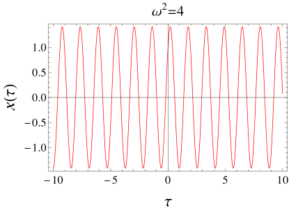
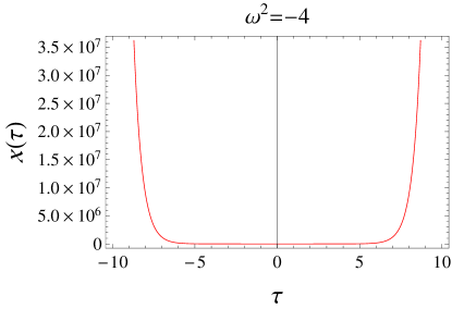
Figure 1: The graphical behavior of the solution of Eq.(24) with different values of $\omega^{2}$.

This equation shows stable and unstable configurations of a thin-shell that depends on $\omega^{2}$. It is found that thin-shell expresses oscillation about $x=0$ for $\omega^{2}>0$ as shown in the left plot of Figure 1. Hence, the developed structure indicates oscillation about the equilibrium shell radius ($x=0\Rightarrow a=a_{0}$) and remains stable. This leads to a stable configuration of a thin-shell. We can write this condition as

$$\frac{d^{2}V(a)}{da^{2}}|_{a=a_{0}}>0.$$ (25)

If $\omega^{2}<0$, then the shell radius represents the exponential behavior which corresponds to the unstable behavior as shown in the right plot of Figure 1. The respective condition for the unstable configuration can be expressed as

$$\frac{d^{2}V(a)}{da^{2}}|_{a=a_{0}}<0.$$ (26)

Hence, the developed structure shows stable configuration against the radial perturbation for an equilibrium shell radius $a=a_{0}$, if

$$V(a_{0})=0,\quad V^{\prime}(a_{0})=0,\quad V^{\prime\prime}(a_{0})>0.$$ (27)

The shell’s motion along the radial direction vanishes at equilibrium shell radius, i.e., $\dot{a}_{0}=0=\ddot{a}_{0}$. If $V^{\prime\prime}(a_{0})<0$, then it shows unstable behavior while it is unpredictable when $V^{\prime\prime}(a_{0})=0$.

We would like to mention here that we have explored the stability of thin-shell gravastar in the background of interior dS and exterior regular BHs (Bardeen and Bardeen-dS BHs) (Sharif and Javed 2020). We have investigated the physical viability of the developed model through the energy conditions and explored its stability by using radial perturbation about the equilibrium shell radius. We have found that thin-shell gravastars show large stable regions for the Bardeen-dS BH as compared to the Bardeen BH. We have concluded that stable regions exist near the formation of the expected event horizon (Sharif and Javed 2020). The present manuscript is devoted to exploring the outcomes of the developed structure filled with stiff and dust fluid distributions. Here, we extend this work for the possible existence of bounded excursion gravastar with different choices of interior and exterior geometries. The stable bounded excursion is a less stringent concept to determine the stability of a geometrical structure. According to this notion, the shell’s motion must be bounded in between an interval $(a_{1},a_{2})$ with $a_{1}<a_{2}$ and follows the conditions

$$V(a_{1})=0,\quad V^{\prime}(a_{1})\leq 0,\quad V(a_{2})=0,\quad V^{\prime}(a_{2})\geq 0,$$ (28)

with $V(a)<0$, $\forall a\in(a_{1},a_{2})$.

We use this approach to discuss the outcomes of the geometrical structure by using the potential function and its derivative with respect to the shell radius. For this purpose, we solve simultaneously the following equations $V(m_{c},Q_{c},L_{ic},L_{ec},a_{c})=0=V^{\prime}(m_{c},Q_{c},L_{ic},L_{ec},a_{c})$ and evaluate the respective critical values of the physical parameters like $m_{c}$, $Q_{c}$, $L_{ic}$, $L_{ec}$ and $a_{c}$. The critical value of the shell radius ($a_{c}$) demonstrates the position of the shell at which it has neither expanding nor collapsing nature. These points of the geometrical structure can also be referred to as the saddle points. Similarly, the remaining critical values of the physical parameters also explain the position of the shell at saddle points. Due to complicated nature of Eq.(22), we cannot manipulate it analytically and hence consider some special cases. The specific values of physical parameters lead to different interior and exterior geometries of the shell. We do not consider the case $m=\Lambda_{i}=\Lambda_{e}=0$ as it corresponds to the Minkowski spacetime in both interior as well as exterior regions and hence thin-shell disappears. Following special cases recover the previous results (Rocha et al 2008a; 2008b; Chan et al 2009b; 2010).

• $m=0=\Lambda_{e}$ and $\Lambda_{i}\neq 0$.

• $m=0=\Lambda_{i}$ and $\Lambda_{e}\neq 0$.

• $m\neq 0$, $Q=0$ and $\Lambda_{i}=0=\Lambda_{e}$.

• $m\neq 0$, $Q=0$ and $\Lambda_{i}\neq 0\neq\Lambda_{e}$.

Here, we consider the following cases

• $m\neq 0\neq Q$ and $\Lambda_{i}=0=\Lambda_{e}$.

• $m\neq 0\neq Q$, $\Lambda_{i}\neq 0$ and $\Lambda_{e}=0$.

• $m\neq 0\neq Q$ and $\Lambda_{i}\neq 0\neq\Lambda_{e}$.

In the following, we explore a suitable case for the construction of bounded excursion gravastar through effective potential with two different choices of matter distribution at the shell, i.e., stiff ($\beta=0$) and dust ($\beta=1$) fluids.

3.1 Stiff Fluid Shell

Here, we assume that the shell of the constructed model is filled with stiff fluid and the effective potential for such a matter distribution can be obtained by using $\beta=0$ in Eq.(22). The corresponding expressions of the potential function and its derivative to $a$ is given as

$$V(a) = \frac{1}{2}+\frac{a^{10}}{4L_{e}^{2}L_{i}^{2}}-\frac{a^{10}}{8L_{e}^{4}}-\frac{a^{10}}{8L_{i}^{4}}-\frac{1}{8a^{6}}-\frac{a^{2}}{4L_{e}^{2}}-\frac{a^{2}m}{2\left(a^{2}+Q^{2}\right)^{3/2}}-\frac{a^{2}}{4L_{i}^{2}}$$ (29)

$$- \frac{a^{10}m}{2\left(a^{2}+Q^{2}\right)^{3/2}L_{e}^{2}}+\frac{a^{10}m}{2\left(a^{2}+Q^{2}\right)^{3/2}L_{i}^{2}}-\frac{a^{10}m^{2}}{2\left(a^{2}+Q^{2}\right)^{3}},$$

$$V^{\prime}(a) = \frac{5a^{9}}{2L_{e}^{2}L_{i}^{2}}-\frac{5a^{9}}{4L_{e}^{4}}-\frac{am}{\left(a^{2}+Q^{2}\right)^{3/2}}+\frac{3a^{11}m}{2\left(a^{2}+Q^{2}\right)^{5/2}L_{e}^{2}}-\frac{5a^{9}}{4L_{i}^{4}}-\frac{a}{2L_{i}^{2}}$$ (30)

$$+ \frac{3}{4a^{7}}-\frac{3a^{11}m}{2\left(a^{2}+Q^{2}\right)^{5/2}L_{i}^{2}}+\frac{3a^{11}m^{2}}{\left(a^{2}+Q^{2}\right)^{4}}-\frac{5a^{9}m}{\left(a^{2}+Q^{2}\right)^{3/2}L_{e}^{2}}$$

$$+ \frac{5a^{9}m}{\left(a^{2}+Q^{2}\right)^{3/2}L_{i}^{2}}-\frac{5a^{9}m^{2}}{\left(a^{2}+Q^{2}\right)^{3}}-\frac{a}{2L_{e}^{2}}+\frac{3a^{3}m}{2\left(a^{2}+Q^{2}\right)^{5/2}},$$

respectively. These are used to discuss the dynamical configuration of a shell with suitable values of the physical parameters. We solve simultaneously $V(a)=0$ and $V^{\prime}(a)=0$ for suitable values of $Q$. The solutions of this system are used to determine the shell’s radius at which the shell neither collapses nor expands. These values are also referred to as critical values of the physical parameters. We have obtained the respective critical values of physical parameters like $a_{c}$, $Q_{c}$, $m_{c}$, $L_{ic}$ and $L_{ec}$ for stiff matter distribution at the constructed shell as shown in Table 1. This table also explains the outcomes of the developed structure with different choices of interior and exterior geometries. We explore the graphical behavior of the potential function corresponding to critical values of physical parameters. Here, we use three different possibilities to explore the stable configuration of the developed structure for the critical values, i.e., $m_{1}<m_{c}<m_{2}$, $Q_{1}<Q_{c}<Q_{2}$, $L_{i1}<L_{ic}<L_{i2}$ and $L_{e1}<L_{ec}<L_{e2}$. To obtain suitable results, we compare the graphical behavior through these choices, i.e., the system behavior for critical values and other values that are greater or smaller than critical values. For this purpose, we assume suitable values of the physical parameters close to the critical ones.

Case (i): $m\neq 0\neq Q$ and $\Lambda_{i}=0=\Lambda_{e}$

This case denotes the internal flat region with external Bardeen BH and the respective critical values of physical parameters are shown in Table 1. For these values, the potential function shows neither expansion nor collapse at $a=a_{c}$ as shown in Figures 2-4. It is found that the effective potential approaches to $-\infty$ as $a\rightarrow\infty$ or $0$. Thus the strictly negative behavior of potential function shows the formation of BH as an outcome of the gravitational collapse of a star. We also analyze the effects of mass and charge on the dynamical configuration of the star. Here, we obtain the results for different choices of mass and charge by considering $m<m_{c}$, $m=m_{c}$, $m>m_{c}$ and $Q<Q_{c}$, $Q=Q_{c}$, $Q>Q_{c}$ as shown in the left and right plots of Figures 2-4, respectively.

Table 1: Critical values of physical parameters and outcomes of the developed structure for a stiff fluid shell with different choices of internal and external geometries. Here, we use the internal region (IR), external region (ER), structure (St), figures (Fig.) flat region (FR), Bardeen BH (B), Bardeen-dS BH (BdS), the normal star (NS), and gravastar (GS).

Final outcomes of the developed structure for stiff fluid shell ($\beta=0$)
$Q_{c}$	$a_{c}$	$m_{c}$	$L_{ic}$	$L_{ec}$	IR	ER	St	Fig
0.4	1.041184	0.631676	-	-	FR	B	BH	2
0.5	1.026782	0.702327	-	-	FR	B	BH	3
2.5	0.937496	10.33415	-	-	FR	B	BH	4
0.4	1.041184	0.422023	2.944657	-	dS	B	GS	5
0.5	1.026782	0.435288	2.574298	-	dS	B	GS	6
2.5	0.937496	10.33415	3.8117$\times 10^{7}$	-	DS	B	GS	7
0.4	1.041184	0.549544	2.944657	2.793761	dS	BdS	GS	8
0.5	1.026782	0.572372	2.574298	2.357312	dS	BdS	GS	9
2.5	0.937496	10.33415	3.8117$\times 10^{7}$	1.67201$\times 10^{7}$	dS	BdS	GS	10

For $m<m_{c}$, the potential function has two real roots say $a_{1}$ and $a_{2}$ with $a_{1}<a_{2}$. It is found that $V(a)<0$ for $a<a_{1}$, $V(a)>0$ for $a_{2}<a<a_{1}$ and $V(a)<0$ for $a>a_{2}$. This represents the unstable structure under small perturbation which leads to star either collapses until $a=0$ and leaves behind a Bardeen BH or expands forever to form a flat spacetime (left plot of Figure 2). For $m=m_{c}$, the star shows collapsing behavior for $a<a_{c}$ until $a\rightarrow 0$ that leads to Minkowski spacetime and stops collapse or expansion at $a=a_{c}$ and then collapses continuously for $a>a_{c}$. The potential function is strictly negative for $m>m_{c}$ which corresponds to the formation of BH as an output of the collapse of a star as shown in Figure 2. We have the similar behavior of potential function for different values of charge (Figures 2-4). Hence, this case gives unstable stable structure under small perturbation for every choice of the physical parameters.

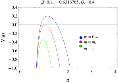
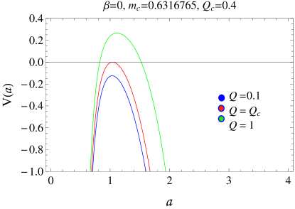
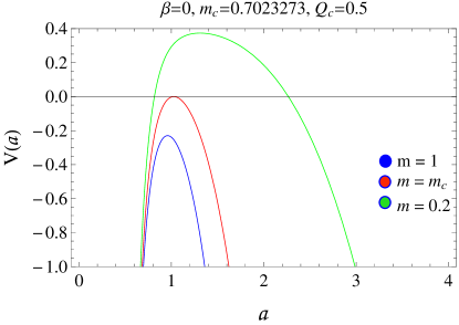
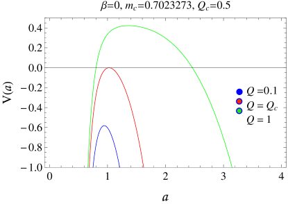
Figure 2: The potential function for interior flat and exterior Bardeen BH with different values of mass (left plot) and charge (right plot).

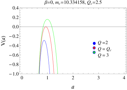
Figure 3: The potential function for interior flat and exterior Bardeen BH with different values of mass (left plot) and charge (right plot).

Figure 4: The potential function for interior flat and exterior Bardeen BH with different values of mass (left plot) and charge (right plot).

Case (ii): $m\neq 0\neq Q$, $\Lambda_{i}\neq 0$ and $\Lambda_{e}=0$

This case represents the internal dS region with external Bardeen BH. The corresponding critical values of physical parameters are given in Table 1. In this case, we observe the effects of mass and $L_{i}$ on the final configuration of the developed structure as shown in Figures 5-7. This case represents the possibility of the existence of bounded excursion gravastar for a suitable choice of physical parameters. It is found that the star shows collapsing behavior for critical values of the physical parameters as given in Table 1. The potential function has four real roots for specific choices of $m$ and $L_{i}$ with $0<a_{1}<a_{2}<a_{3}<a_{4}$. If $a<a_{1}$, then the potential function approaches to $-\infty$ as $a\rightarrow 0$ that represents the flat spacetime. If $a_{1}<a<a_{2}$, then $V(a)>0$ which is unstable under small perturbation. If $a_{2}<a<a_{3}$, then $V(a)<0$ implying the existence of stable bounded excursion gravastar. If $a_{3}<a<a_{4}$, then again $V(a)>0$ which shows unstable configuration under small perturbation. The potential function again approaches $-\infty$ as $a\rightarrow\infty$ for $a>a_{4}$ which leads to the formation of BH (Figures 5-7). It is found that the region of the existence of gravastar is very small as compared to the BHs. Hence, the dynamical model cannot completely exclude the possibility of the formation of gravastar and BH structures. If the gravastar model exists then there is also a possibility for the existence of BH and vice versa. It is also interesting to mention here that the regions of stable bounded excursion gravastar are enhanced by increasing mass and $L_{i}$.

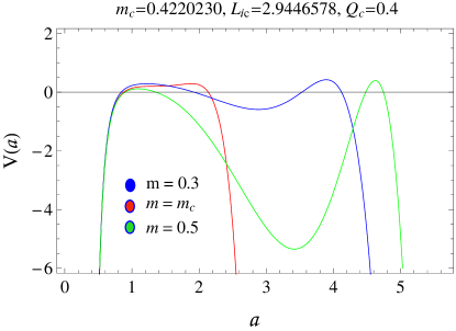
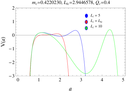
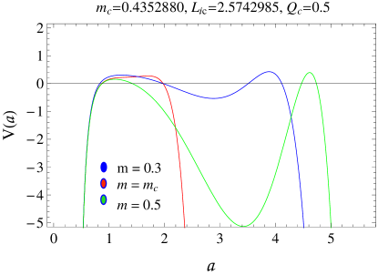
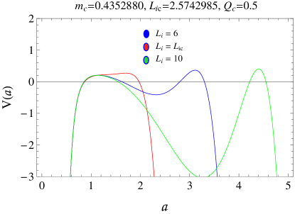
Figure 5: The potential function for interior dS spacetime and exterior Bardeen BH with different values of mass (left plot) and $L_{i}$ (right plot).

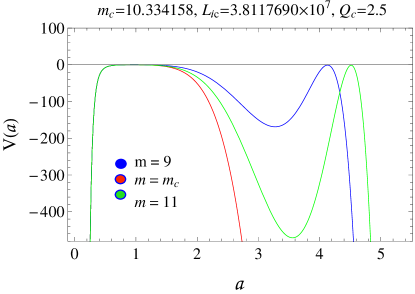
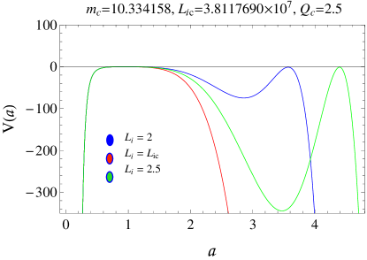
Figure 6: The potential function for interior dS spacetime and exterior Bardeen BH with different values of mass (left plot) and $L_{i}$ (right plot).

Figure 7: The potential function for interior dS spacetime and exterior Bardeen BH with different values of mass (left plot) and $L_{i}$ (right plot).

Case (iii): $m\neq 0\neq Q$ and $\Lambda_{i}\neq 0\neq\Lambda_{e}$

This is the general case that leads to the internal dS region and external Bardeen-dS BH. The critical values of physical parameters are given in Table 1. To avoid the presence of an event horizon in the developed structure, it is found that $\Lambda_{i}>\Lambda_{e}$ which corresponds to $L_{e}>L_{i}$. It is observed that the obtained critical values of $L_{i}$ and $L_{e}$ do not satisfy the required inequality ($L_{e}>L_{i}$). Hence, the behavior of stars must be collapsing for these choices of physical parameters. The graphical behavior of potential function shows that the developed structure represents collapse leading to BH if $L_{e}<L_{i}$ (Figures 8-10). Therefore, we assume the particular choice of $L_{i}$ and $L_{e}$ with $L_{e}>L_{i}$ for different values of $L_{e}$ and $Q$. It is found that the developed structure shows the existence of stable bounded excursion gravastar if $L_{e}>L_{i}$. The regions of stable bounded excursion gravastar increase by increasing $L_{e}$ and $Q$.

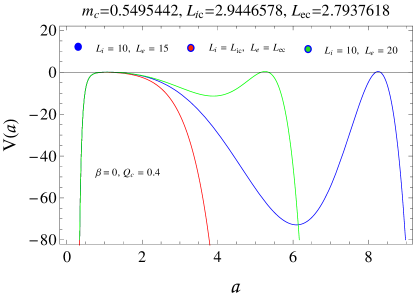
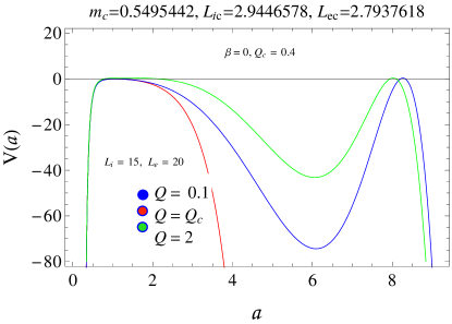
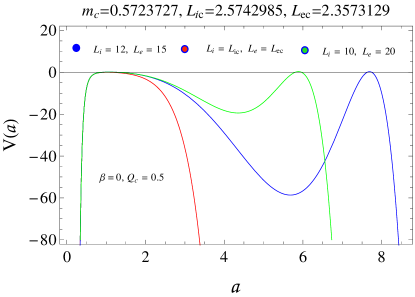
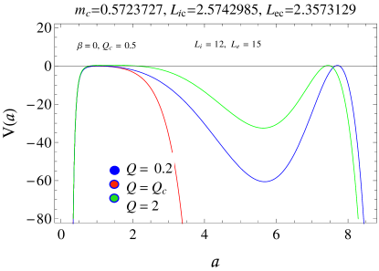
Figure 8: The potential function for interior dS spacetime and exterior Bardeen-dS BH with different values of $L_{i}$, $L_{e}$ (left plot) and charge (right plot).

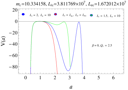
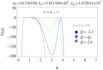
Figure 9: The potential function for interior dS spacetime and exterior Bardeen-dS BH with different values of $L_{i}$, $L_{e}$ (left plot) and charge (right plot).

Figure 10: The potential function for interior dS spacetime and exterior Bardeen-dS BH with different values of $L_{i}$, $L_{e}$ (left plot) and charge (right plot).

3.2 Dust Fluid Shell

Here, we explore the results in the presence of dust fluid distribution at the shell. The corresponding expressions of the potential function and its derivative can be written as

$$V(a) = \frac{1}{2}+\frac{a^{6}}{4L_{e}^{2}L_{i}^{2}}-\frac{a^{6}}{8L_{e}^{4}}-\frac{a^{6}}{8L_{i}^{4}}-\frac{a^{2}}{4L_{e}^{2}}-\frac{a^{2}}{4L_{i}^{2}}-\frac{a^{2}m}{2\left(a^{2}+Q^{2}\right)^{3/2}}-\frac{1}{8a^{2}}$$ (31)

$$- \frac{a^{6}m}{2\left(a^{2}+Q^{2}\right)^{3/2}L_{e}^{2}}+\frac{a^{6}m}{2\left(a^{2}+Q^{2}\right)^{3/2}L_{i}^{2}}-\frac{a^{6}m^{2}}{2\left(a^{2}+Q^{2}\right)^{3}},$$

$$V^{\prime}(a) = \frac{3a^{5}}{2L_{e}^{2}L_{i}^{2}}-\frac{3a^{5}}{4L_{e}^{4}}-\frac{3a^{5}}{4L_{i}^{4}}+\frac{1}{4a^{3}}-\frac{am}{\left(a^{2}+Q^{2}\right)^{3/2}}+\frac{3a^{7}m}{2\left(a^{2}+Q^{2}\right)^{5/2}L_{e}^{2}}$$ (32)

$$- \frac{3a^{7}m}{2\left(a^{2}+Q^{2}\right)^{5/2}L_{i}^{2}}+\frac{3a^{7}m^{2}}{\left(a^{2}+Q^{2}\right)^{4}}-\frac{3a^{5}m}{\left(a^{2}+Q^{2}\right)^{3/2}L_{e}^{2}}-\frac{3a^{5}m^{2}}{\left(a^{2}+Q^{2}\right)^{3}}$$

$$+ \frac{3a^{5}m}{\left(a^{2}+Q^{2}\right)^{3/2}L_{i}^{2}}+\frac{3a^{3}m}{2\left(a^{2}+Q^{2}\right)^{5/2}}-\frac{a}{2L_{e}^{2}}-\frac{a}{2L_{i}^{2}},$$

respectively. The respective critical values for different choices of interior and exterior regions are expressed in Table 2. We choose suitable values of charge for which the system shows real critical values of physical parameters.

Table 2: Critical values of physical parameters and outcomes of the developed structure for dust fluid shell with different internal and external geometries.

Final outcomes of developed structure for dust fluid shell ($\beta=1$)
$Q_{c}$	$a_{c}$	$m_{c}$	$L_{ic}$	$L_{ec}$	IR	ER	St	Fig
0.7	1.918218	0.891839	-	-	FR	B	NS	11
0.8	2.981319	0.923782	-	-	FR	B	NS	12
1.5	0.703307	3.778338	-	-	FR	B	BH	13
0.7	1.021781	0.909516	6.64462$\times 10^{7}$	-	dS	B	GS	14
0.8	2.981319	1.636369	15.37334	-	dS	B	GS	15
1.5	12.79669	0.980800	4.15909$\times 10^{9}$	-	dS	B	GS	16
0.7	1.918218	0.880891	8.692764	10.64767	dS	BdS	GS	17
0.8	2.981319	0.916398	15.37334	17.40656	dS	BdS	GS	18
1.5	12.79669	0.978446	109.3384	112.3030	dS	BdS	GS	19

Case (i): $m\neq 0\neq Q$ and $\Lambda_{i}=0=\Lambda_{e}$

The results of the collapse of a shell with an internal flat and external Bardeen BH is shown in Figures 11-13. The the potential function represents the stable configuration of the developed structure for every value of mass and charge which denotes the presence of normal star (Figures 11 and 12). The shell shows collapsing behavior ($V(a)<0$) for small values of shell radius and then shows expansion ($V(a)>0$). Figure 13 indicates the collapsing configuration which leads to the formation of BHs. There is no possible way to develop gravastar for every choice of physical parameters.

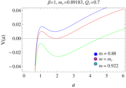
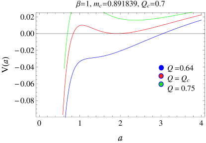
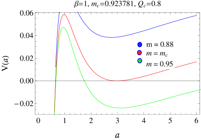
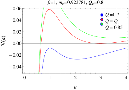
Figure 11: The potential function for interior flat and exterior Bardeen BH with different values of mass (left plot) and charge (right plot).

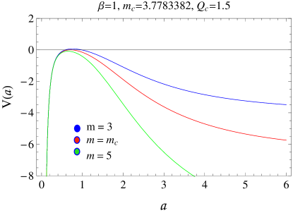
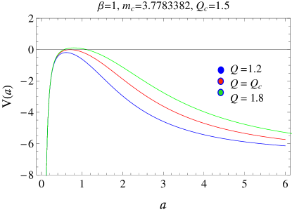
Figure 12: The potential function for interior flat and exterior Bardeen BH with different values of mass (left plot) and charge (right plot).

Figure 13: The potential function for interior flat and exterior Bardeen BH with different values of mass (left plot) and charge (right plot).

Case (ii): $m\neq 0\neq Q$, $\Lambda_{i}\neq 0$ and $\Lambda_{e}=0$

Here we take the collapse of internal dS and external Bardeen BH through critical values given in Table 2. This is the most suitable case for the existence of stable bounded excursion gravastar. The stable gravastar must exist for the choice of considered critical values (Table 2) as shown in Figures 14-16. The potential function has two real roots as $0<a_{1}<a_{2}$. If $a<a_{1}$, then the potential function approaches to $-\infty$ as $a\rightarrow 0$ that represents the flat spacetime. If $a_{1}<a<a_{2}$, then the potential function is less than zero and hence expresses the existence of stable bounded excursion gravastar. If $a_{2}<a$, then $V(a)$ approaches to plus or minus infinity that express the expansion and collapsing behavior as $a\rightarrow\infty$. It is found that the choice of Bardeen BH as an exterior geometry of shell filled with dust fluid provides stable bounded excursion gravastar as compared to the choice of Schwarzschild/ Schwarzschild dS/RN geometries (Rocha et al 2008a; 2008b; Chan et al 2009b; 2010). Hence, this is more suitable for the construction of stable gravastar with a dust shell.

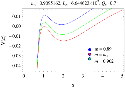
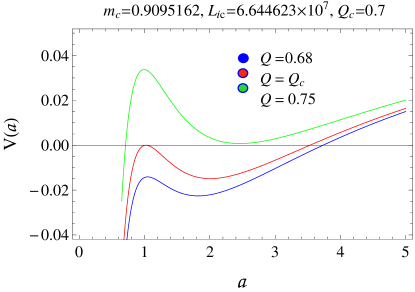
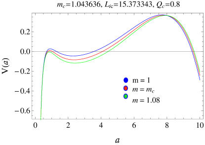
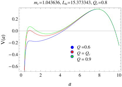
Figure 14: The potential function for interior dS spacetime and exterior Bardeen BH with different values of mass (left plot) and charge (right plot).

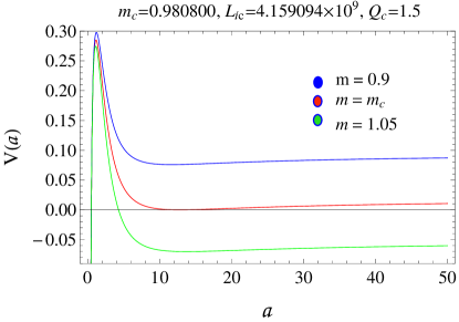
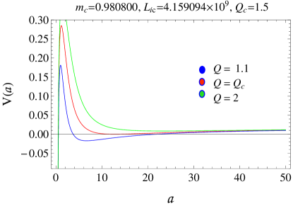
Figure 15: The potential function for interior dS spacetime and exterior Bardeen BH with different values of mass (left plot) and charge (right plot).

Figure 16: The potential function for interior dS spacetime and exterior Bardeen BH with different values of mass (left plot) and charge (right plot).

Case (iii): $m\neq 0\neq Q$ and $\Lambda_{i}\neq 0\neq\Lambda_{e}$

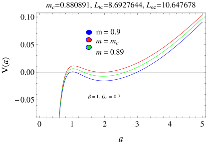
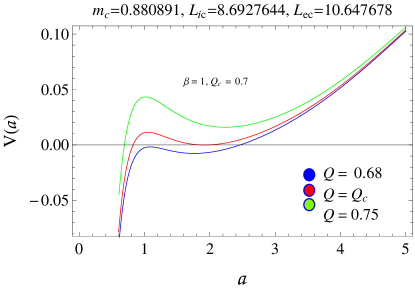
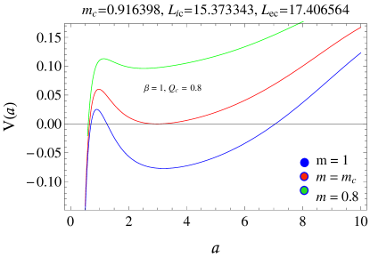
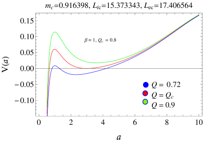
Figure 17: The potential function for interior dS spacetime and exterior Bardeen-dS BH with different values of mass (left plot) and charge (right plot).

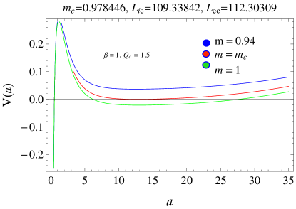
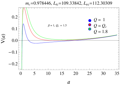
Figure 18: The potential function for interior dS spacetime and exterior Bardeen-dS BH with different values of mass (left plot) and charge (right plot).

Figure 19: The potential function for interior dS spacetime and exterior Bardeen-dS BH with different values of mass (left plot) and charge (right plot).

We consider the internal dS region and external Bardeen-dS BH. The critical values (Table 2) follow the inequality $L_{e}>L_{i}$ with every considered choice of $Q$. Hence, the developed structure is suitable to eliminate the presence of an event horizon and singularity for critical values. The graphical behavior of the potential function shows the expanding behavior which gives information about the existence of stable gravastar near the suitable critical values of physical parameters (Figures 17-19). Hence, the stable gravastar must exist for the different choices of $m$ and $Q$.

4 Final Remarks

This work is the extension of stability issues related to the possible existence of stable bounded excursion gravastar from a model consisting of internal dS region, intermediate thin-shell filled with matter distribution followed the EoS $p=(1-\beta)\rho$ and external Schwarzschild dS as well as RN spacetimes (Rocha et al 2008a; 2008b; Chan et al 2009b; 2010). Here, we are interested to explore the existence of bounded excursion gravastar in the background of exterior regular Bardeen and Bardeen-dS BHs. We have used the cut and paste approach to match these spacetimes at the shell. The potential function of the shell filled with matter distribution ($p=(1-\beta)\rho$) can be evaluated through the equation of motion of the shell. The developed framework is investigated through the critical values of physical parameters by solving the following equations $V(a)=0$ and $V^{\prime}(a)=0$, simultaneously. For this purpose, we have considered two types of matter distribution, stiff ($\beta=0$) and dust ($\beta=1$) fluids.

For the stiff fluid shell, the critical values of physical parameters for three different cases are given in Table 1. For the interior flat spacetime and exterior Bardeen BHs, we have obtained the collapsing behavior of the shell which indicates the formation of BHs (Figures 2-4). The interior dS and exterior Bardeen BH represent the region of stable bounded excursion gravastar for a suitable choice of physical parameters. If the gravastar model exists then there is a possibility for the existence of BH and vice versa. We have analyzed that the regions of stable bounded excursion gravastar increase by increasing mass and $L_{i}$ (Figures 5-7). For the interior dS and exterior Bardeen-dS BH, we have obtained that bounded excursion stable gravastar must exist if $L_{i}<L_{e}$ (Figures 8-10). The regions of bounded excursion gravastar increase by enhancing charge and $L_{e}$.

For dust fluid shell, we have obtained the respective critical values of physical parameters (Table 2). There does not exist the possibility of the existence of gravastar for the flat and exterior Bardeen BH (Figures 11-13). The stable structure of bounded excursion gravastar is found for every choice of physical parameters for the interior dS and exterior Bardeen BH (Figures 14-16). The stable bounded excursion gravastar is determined for suitable choices of physical parameters with interior dS and exterior Bardeen-dS BH (Figures 17-19).

We conclude that the gravastar model in the background of regular BHs is more feasible for the existence of a stable configuration of bounded excursion gravastar than the Schwarzschild and RN BHs (Rocha et al 2008a; 2008b; Chan et al 2009b; 2010). These BHs do not provide any region of stable gravastar for the choice of dust shell while our models show stable regions of bounded excursion gravastar. This paper also follows the previous results for the choice of $Q=0$ (Chan et al 2009b).

Conflict of Interest Statement: The authors declare that they do not have any conflict of interest.

References

- [1] Amirabi, Z., Halilsoy, M. and Habib Mazharimousavi, S., 2013, Phys. Rev. D, 88, 124023
- [2] Ayn-Beato, E. and Garca, A., 1998, Phys. Rev. Lett., 80, 5056
- [3] Ayn-Beato, E. and Garca, A., 2000, Phys. Lett. B, 493, 149
- [4] Banerjee, A., Rahaman, F., Islam, S. and Govender, M., 2016, Eur. Phys. J. C, 76, 34
- [5] Banerjee, A., Villanueva, J.R., Channuie, P. and Jusuf, K., 2018, Chinese Phys. C, 42, 115101
- [6] Bardeen, J.M., 1968, Proceedings of GR5 (Tiflis, USSR), 174
- [7] Bhatti, M.Z., Yousaf, Z. and Rehman, A., 2020, Phys. Dark Universe, 29, 100561
- [8] Brady, P.R., Louko, J. and Poisson, E., 1991, Phys. Rev. D, 44, 1891
- [9] Bronnikov, K.A., 2001, Phys. Rev. Lett., 85, 4641
- [10] Carter, B.M.N., 2005, Class. Quantum Grav., 22, 4551
- [11] Chapline, G., Hohlfeld, E., Laughlin, R.B. and Santiago, D.I., 2003, Int. J. Mod. Phys. A, 18, 3587
- [12] Chan, R., da Silva, M.F.A., Rocha, P., and Wang, A., 2009a, J. Cosmol. Astropart. Phys., 03, 10
- [13] Chan, R., da Silva, M.F.A. and Rocha, P., 2009b, J. Cosmol. Astropart. Phys., 12, 17
- [14] Chan, R. and da Silva, M.F.A., 2010, J. Cosmol. Astropart. Phys., 07, 29
- [15] Chan, R., da Silva, M.F.A. and Rocha, P., 2011a, Gen. Relativ. Gravit., 43, 2223
- [16] Chan, R., et al., 2011b, J. Cosmol. Astropart. Phys., 10, 013
- [17] Copeland, E.J., Sami, M. and Tsujikawa, S., 2006, Int. J. Mod. Phys. D, 15, 1753
- [18] Das, A., 2020, Nucl. Phys. B, 954, 114986
- [19] DeBenedictis, A., et al., 2006, J. Cosmol. Astropart. Phys., 23, 2303
- [20] Dias, G.A.S. and Lemos, J.P.S., 2010, Phys. Rev. D, 82, 084023
- [21] Eiroa, E.F. and Simeone, C., 2007, Phys. Rev. D, 76, 024021
- [22] Fernando, S., 2017, Int. J. Mod. Phys. D, 26, 1750071
- [23] Forghani, S.D., Habib Mazharimousavi, S. and Halilsoy, M., 2018, Eur. Phys. J. C, 78, 469
- [24] Ghosh, S., Rahaman, F., Guha, B.K. and Ray, S., 2017, Phys. Lett. B, 767, 380
- [25] Halilsoya, M., Övgün, A. and Mazharimousavi, S.H., 2014, Eur. Phys. J. C, 74, 2796
- [26] Hayward, S.A., 2006, Phys. Rev. Lett., 96, 031103
- [27] Horvat, D. and Iliji, S., 2007, J. Cosmol. Astropart. Phys., 24, 5637
- [28] Horvat, D., Sasa Ilijic, S. and Marunovic, A., 2009, Class. Quantum Grav., 26, 025003
- [29] Horvat, D., Ilijic, S. and Marunovic, A., 2011, Class. Quantum Grav., 28, 195008
- [30] Israel, W., 1966, Nuovo Cim. B Ser., 44, 1
- [31] Israel, W., 1967, Nuovo Cim. B Ser., 48, 463
- [32] Martinez, E.A., 1996, Phys. Rev. D 53, 7062
- [33] Mazharimousavi, S.H., Halilsoy, M. and Hamad, A.S.N., 2017, Int. J. Mod. Phys. D, 26, 1750158
- [34] Mazharimousavi, S.H., Halilsoy, M. and Amirabi, Z., 2010, Phys. Rev. D, 81, 104002
- [35] Mazur, P. and Mottola, E., 2001, arXiv: gr-qc/0109035
- [36] Mazur, P. and Mottola, E., 2004, Proc. Nat. Acad. Sci., 101, 9545
- [37] Övgün, A., Banerjee, A. and Jusufi, K., 2017, Eur. Phys. J. C, 77, 566
- [38] Lake, K., 1979, Phys. Rev. D, 19, 2847
- [39] LeMaitre, P. and Poisson, E., 2019, Amer. J. Phys., 87, 961
- [40] Lobo, F.S.N. and Arellano, A.V.B., 2007, Class. Quant. Grav., 24, 1069
- [41] Lobo, F.S.N. and Crawford, P., 2004, Class. Quantum Grav., 21, 391
- [42] Lobo, F.S.N. and Garattini, R., 2013, J. High Energy Phys., 1312, 065
- [43] Lobo, F.S.N., 2006, Class. Quantum Grav., 23, 1525
- [44] Rahaman, F., Usmani, A.A., Ray, S. and Islam, S., 2012a, Phys. Lett. B, 707, 319
- [45] Rahaman, F., Usmani, A.A., Ray, S. and Islam, S., 2012b, Phys. Lett. B, 717, 1
- [46] Rocha, P., et al., 2008a, J. Cosmol. Astropart. Phys. 06, 25
- [47] Rocha, P., et al., 2008b, J. Cosmol. Astropart. Phys., 11, 010
- [48] Shamir, M.F. and Ahmad, M., 2018, Phys. Rev. D, 97, 104031
- [49] Sharif, M. and Javed, F., 2016, Gen. Relativ. Gravit., 48, 158
- [50] Sharif, M. and Javed, F., 2019, Astrophys. Space. Sci., 364, 179
- [51] Sharif, M. and Javed, F., 2020, Ann. Phys. 415, 168124
- [52] Sharif, M. and Waseem, A., 2019, Astrophys. Space Sci., 364, 189
- [53] Visser, M. and Wiltshire, D.L., 2004, Class. Quantum Grav., 21, 1135
- [54] Visser, M., 1989, Phys. Rev. D, 39, 3182
- [55] Yousaf, Z., et al., 2019, Phys. Rev. D, 100, 024062
- [56] Yousaf, Z., 2020, Phys. Dark Universe 28, 100509
- [57] Wald, R.M., 2001, Living Rev. Real., 4, 6
- [58]