Rigid indecomposable modules in Grassmannian cluster categories

Abstract.

The coordinate ring of the Grassmannian variety of $k$-dimensional subspaces in $\mathbb{C}^{n}$ has a cluster algebra structure with Plücker relations giving rise to exchange relations. In this paper, we study indecomposable modules of the corresponding Grassmannian cluster categories ${\rm CM}(B_{k,n})$.  Jensen, King, and Su have associated a Kac-Moody root system $J_{k,n}$ to ${\rm CM}(B_{k,n})$ and shown that in the finite types, rigid indecomposable modules correspond to roots. In general, the link between the category ${\rm CM}(B_{k,n})$ and the root system $J_{k,n}$ remains mysterious and it is an open question whether indecomposables always give roots. In this paper, we provide evidence for this association in the infinite types: we show that every indecomposable rank 2 module corresponds to a root of the associated root system. We also show that indecomposable rank 3 modules in ${\rm CM}(B_{3,n})$ all give rise to roots of $J_{3,n}$. For the rank 3 modules in ${\rm CM}(B_{3,n})$ corresponding to real roots, we show that their underlying profiles are cyclic permutations of a certain canonical one. We also characterize the rank 3 modules in ${\rm CM}(B_{3,n})$ corresponding to imaginary roots. By proving that there are exactly 225 profiles of rigid indecomposable rank 3 modules in ${\rm CM}(B_{3,9})$ we confirm the link between the Grassmannian cluster category and the associated root system in this case. We conjecture that the profile of any rigid indecomposable module in ${\rm CM}(B_{k,n})$ corresponding to a real root is a cyclic permutation of a canonical profile.

1. Introduction

Consider the homogeneous coordinate ring $\mathbb{C}[\mathrm{Gr}(2,n)]$ of the Grassmannian of 2-dimensional subspaces of $\mathbb{C}^{n}$. This is one of the key initial examples of Fomin and Zelevinsky’s theory of cluster algebras, [11, §12.2]: the cluster variables are the Plücker coordinates, the exchange relations arise from the short Plücker relations, and clusters are in bijection with triangulations of a convex $n$-gon. Scott then proved in [25] that this cluster structure can be generalized to the coordinate ring $\mathbb{C}[\mathrm{Gr}(k,n)]$, where additional cluster variables appear (in general, infinitely many) and more exchange relations. This has sparked a lot of research activities in cluster theory, e.g. [26, 13, 15, 14, 24, 7, 16, 23, 12].

In particular, Jensen, King and Su showed in [16] that the category ${\rm CM}(B_{k,n})$ of Cohen-Macaulay modules over a quotient $B_{k,n}$ of a preprojective algebra of affine type $A$ provides an additive categorification of Scott’s cluster algebra structure. The category ${\rm CM}(B_{k,n})$ is called the Grassmannian cluster category. They also show that there is a cluster character on this category, sending rigid indecomposable objects to cluster variables ([16, Section 9]). Without loss of generality, we will assume $1\leq k\leq n/2$ from now on.

Through this categorification, the classification of rigid indecomposable modules in ${\rm CM}(B_{k,n})$ (i.e., indecomposable modules $M$ with Ext${}^{1}(M,M)=0$) becomes an important tool towards characterising cluster variables in $\mathbb{C}[\mathrm{Gr}(k,n)]$ as well as in the classification of real prime modules of quantum affine algebras of type $A$, [15, 18].

In this paper, we study indecomposable modules of ${\rm CM}(B_{k,n})$ with the goal of providing an understanding of the associated cluster algebras. A first contribution to this is the fact that in the infinite types, all components in the Auslander-Reiten quiver are tubes, Proposition 2.11. With this, we have some control over certain types of indecomposable modules.

Among the indecomposable modules are the rank 1 modules which are known to be in bijection with $k$-subsets of $\{1,2,\dots,n\}$. These are the building blocks of the category as any module in ${\rm CM}(B_{k,n})$ can be filtered by rank 1 modules (see Section 2.1). Using this, in [16, Section 8], a map is defined from indecomposable modules of ${\rm CM}(B_{k,n})$ to a root lattice by associating a module with its class in the Grothendieck group and identifying the latter with a root lattice (see Section 2.4). Let $J_{k,n}$ be the graph with nodes $1,2,\dots,n-1$ on a line and node $n$ attached to node $k$, see Figure 1. If $k=2$ or $k=3$ and $n\in\{6,7,8\}$, $J_{k,n}$ is a Dynkin diagram, in general, it gives rise to a Kac-Moody algebra. In the Dynkin cases, the categories ${\rm CM}(B_{k,n})$ have only finitely many indecomposable objects and they are known to correspond to positive real roots for the associated root system of $J_{k,n}$, [16, Section 2].

Figure 1. The diagram of the root system $J_{k,n}$ associated with $\mathrm{Gr}(k,n)$, we write $\beta$ for $\alpha_{n}$.

In general, it is a very difficult problem to describe the structure of the category or to classify indecomposable modules in ${\rm CM}(B_{k,n})$. In contrast to the finite case, it is not clear how the correspondence between modules in the Grassmannian cluster categories and the root system arises. However, Jensen, King and Su [16] suspect that the classes of rigid indecomposable modules indeed are roots for $J_{k,n}$. Evidence for this was given in the small rank cases for certain infinite cases in  [5]. The authors give a construction of rank 2 modules via short exact sequences, and find conditions that filtration factors of these modules have to fulfill. They also show that ${\rm CM}(B_{k,n})$ has at most $2{n\choose 6}{n-6\choose k-3}$ (profiles of) rigid indecomposable rank 2 modules which correspond to real roots. Here, we also consider the imaginary roots and show in Theorem 4.7 (2) that there are at least

$$N_{k,n}=\sum_{r=3}^{k}\left(\frac{2r}{3}\cdot p_{1}(r)+2r\cdot p_{2}(r)+4r\cdot p_{3}(r)\right)\cdot{n\choose 2r}{n-2r\choose k-r}$$

profiles of rigid rank 2 indecomposable modules in ${\rm CM}(B_{k,n})$, where $p_{i}(r)$ is the number of partitions $r=r_{1}+r_{2}+r_{3}$ such that $r_{1},r_{2},r_{3}\in\mathbb{Z}_{\geq 1}$ and $|\{r_{1},r_{2},r_{3}\}|=i$. Furthermore, every rank 2 indecomposable module where the rims of the filtration factors form three rectangular boxes is rigid.

Moreover, any indecomposable rank 2 module corresponds to a root of $J_{k,n}$ and for $k=3$, we show that all rank 3 modules in ${\rm CM}(B_{3,n})$ map to roots for $J_{3,n}$.

Theorem 1 (Lemma 4.6 and Theorem 5.6).

(1) Every indecomposable rank $2$ module in ${\rm CM}(B_{k,n})$ corresponds to a root for $J_{k,n}$.
(2) Every indecomposable module of rank $3$ in ${\rm CM}(B_{3,n})$ corresponds to a root for $J_{3,n}$.

Recall that the modules in ${\rm CM}(B_{k,n})$ can be filtered by rank 1 modules which in turn correspond to $k$-subsets of $[n]=\{1,\ldots,n\}$ (see Section 2.1). The profile of a module is the collection of $k$-subsets corresponding to rank 1 modules in the generic filtration ([16, §8]). If the filtration of $M$ has rank 1 factors $I_{1},\dots,I_{m}$, for some $m>0$, where the rank 1 module $I_{m}$ is a submodule of $M$, we write $M=I_{1}\mid I_{2}\mid\dots\mid I_{m}$. We also write $P_{M}$ for the profile of $M$.

We denote by $\mathcal{P}_{k,n}$ the set of profiles of indecomposable modules in ${\rm CM}(B_{k,n})$. Its elements have $m$ rows with $k$ entries in $[n]$.

Let $P\in\mathcal{P}_{k,n}$ be a profile with $m$ rows. Write $P=(P_{ij})$, $1\leq i\leq m$, $1\leq j\leq k$, for the profile $P$ where the entries in every row are written in increasing order. Then $P$ is called weakly column decreasing if for every $j\in[k]$ and every $i\in[m-1]$, $P_{i,j}\geq P_{i+1,j}$. We call $P$ canonical, if $P$ is weakly column decreasing and if, in addition, $P_{m,j}\geq P_{1,j-1}$ for all $j\in[2,k]$. We write $C_{k,n}^{\rm re}$ to denote the set of all canonical profiles in $\mathcal{P}_{k,n}$ such that the corresponding module gives rise to a real root for $J_{k,n}$ (see Section 2.4).

With this notion, we are able to prove the following.

Theorem 2 (Theorem 5.7).

If $M$ is an indecomposable rank $3$ module in ${\rm CM}(B_{3,n})$ such that $M$ corresponds to a real root for $J_{3,n}$, then the profile $P_{M}$ is a cyclic permutation of a canonical profile (i.e., a cyclic permutation of the rows of the profile of $M$ is canonical).

We expect that Theorem 2 is true for all indecomposable modules corresponding to real roots.

Conjecture 3 (Conjecture 5.8).

If $M\in{\rm CM}(B_{k,n})$ is rigid indecomposable and corresponds to a real root for $J_{k,n}$, then $P_{M}$ is a cyclic permutation of a canonical profile.

We have the following result about modules corresponding to imaginary roots.

Theorem 4 (Theorem 5.9).

Suppose that the indecomposable module $M\in{\rm CM}(B_{3,n})$ corresponds to an imaginary root of $J_{3,n}$. Then $P_{M}$ is one of the following:

$$\begin{aligned} i_{1}i_{5}i_{7}\\ \hline\cr\\[-9.0pt] i_{3}i_{6}i_{9}\\ \hline\cr\\[-9.0pt] i_{2}i_{4}i_{8}\end{aligned},\begin{aligned} i_{2}i_{6}i_{8}\\ \hline\cr\\[-9.0pt] i_{1}i_{4}i_{7}\\ \hline\cr\\[-9.0pt] i_{3}i_{5}i_{9}\end{aligned},\begin{aligned} i_{3}i_{7}i_{9}\\ \hline\cr\\[-9.0pt] i_{2}i_{5}i_{8}\\ \hline\cr\\[-9.0pt] i_{1}i_{4}i_{6}\end{aligned},\begin{aligned} i_{1}i_{4}i_{8}\\ \hline\cr\\[-9.0pt] i_{3}i_{6}i_{9}\\ \hline\cr\\[-9.0pt] i_{2}i_{5}i_{7}\end{aligned},\begin{aligned} i_{2}i_{5}i_{9}\\ \hline\cr\\[-9.0pt] i_{1}i_{4}i_{7}\\ \hline\cr\\[-9.0pt] i_{3}i_{6}i_{8}\end{aligned},\begin{aligned} i_{1}i_{3}i_{6}\\ \hline\cr\\[-9.0pt] i_{2}i_{5}i_{8}\\ \hline\cr\\[-9.0pt] i_{4}i_{7}i_{9}\end{aligned},\begin{aligned} i_{2}i_{4}i_{7}\\ \hline\cr\\[-9.0pt] i_{3}i_{6}i_{9}\\ \hline\cr\\[-9.0pt] i_{1}i_{5}i_{8}\end{aligned},\begin{aligned} i_{3}i_{5}i_{8}\\ \hline\cr\\[-9.0pt] i_{1}i_{4}i_{7}\\ \hline\cr\\[-9.0pt] i_{2}i_{6}i_{9}\end{aligned},\begin{aligned} i_{4}i_{6}i_{9}\\ \hline\cr\\[-9.0pt] i_{2}i_{5}i_{8}\\ \hline\cr\\[-9.0pt] i_{1}i_{3}i_{7}\end{aligned},\begin{aligned} i_{1}i_{4}i_{7}\\ \hline\cr\\[-9.0pt] i_{3}i_{6}i_{9}\\ \hline\cr\\[-9.0pt] i_{2}i_{5}i_{8}\end{aligned},\begin{aligned} i_{2}i_{5}i_{8}\\ \hline\cr\\[-9.0pt] i_{1}i_{4}i_{7}\\ \hline\cr\\[-9.0pt] i_{3}i_{6}i_{9}\end{aligned},\begin{aligned} i_{3}i_{6}i_{9}\\ \hline\cr\\[-9.0pt] i_{2}i_{5}i_{8}\\ \hline\cr\\[-9.0pt] i_{1}i_{4}i_{7}\end{aligned},$$

where $1\leq i_{1}<i_{2}<\cdots<i_{9}\leq n$.

Note that for $n=9$, there are exactly 12 indecomposable rank 3 modules corresponding to an imaginary root. The first 9 in the list are rigid and the last three are non-rigid; we show that in this case, there are exactly 225 rigid indecomposable rank 3 modules corresponding to roots of $J_{3,9}$.

For arbitrary $n>9$, we expect that modules such as the last three in the list of Theorem 4 are always non-rigid.

A module $M^{\prime}\in{\rm CM}(B_{k,n})$ is said to be an $a$-shift of the module $M\in{\rm CM}(B_{k,n})$ if the profile of $M^{\prime}$ is obtained from the profile $P$ of $M$ by adding a fixed number (mod $n$) to every entry of $P$ (Definition 2.7).

Theorem 5 (Theorem 6.7 and Corollary 6.8).

Consider the category ${\rm CM}(B_{3,9})$. Every rigid indecomposable rank $3$ module maps to a root of $J_{3,9}$. Among the rigid indecomposable rank $3$ modules, $216$ correspond to a real root and the profile of each of them is a cyclic permutation of a canonical one. Furthermore, there are $9$ modules mapping to an imaginary root and their profiles are all a shift of $\begin{aligned} 157\\ \hline\cr\\[-9.0pt] 369\\ \hline\cr\\[-9.0pt] 248\end{aligned}$.

Theorem 5 is proved by studying the tubes of the Auslander-Reiten quiver of ${\rm CM}(B_{3,9})$ containing rigid rank 3 modules.

We also prove the following result and its dual version (Theorem 6.5). If $I$ is a $k$-subset of $[n]$, we write $L_{I}$ for the corresponding rank 1 module. If $I$ and $J$ are two $k$-subsets, we write $L_{I}\mid L_{J}$ for the rank 2 module with submodule $L_{J}$ and quotient $L_{I}$.

Theorem 6 (Theorem 6.3).

We consider the category ${\rm CM}(B_{3,n})$. Let $I=\{i_{1},i_{2},i_{3}\}$ be a $3$-subset where $i_{j}<i_{j+1}-1$ for $j=1,2,3$ (reducing modulo $n$). Let $X=\{i_{1}+1,i_{2}+1,i_{3}+1\}$ and $Y=\{i_{1}+2,i_{2}+2,i_{3}+2\}$. Then there is an Auslander-Reiten sequence

$$L_{I}\hookrightarrow M\twoheadrightarrow\frac{L_{X}}{L_{Y}}$$

where $M$ is a rank $3$ module. If $M$ is indecomposable, its profile is $X\mid I\mid Y$.

The paper is organized as follows. In Section 2, we recall key definitions and results about Grassmannian cluster categories. In Section 3, we study profiles and show that a weakly column decreasing profile is canonical if and only if any two rows of its profile are interlacing. In Section 4, we give a lower bound for the number of indecomposable rank 2 modules ${\rm CM}(B_{k,n})$ corresponding to roots for $J_{k,n}$. In Section 5, we concentrate on rank 3 modules and study the subspace configurations. In Section 6, we provide short exact sequences to describe the structure of the Auslander-Reiten quiver for ${\rm CM}(B_{3,n})$. We use this to determine the number of rigid indecomposable rank 3 modules in the infinite case ${\rm CM}(B_{3,9})$.

Acknowledgments

We thank Christof Geiss, Alastair King, Matthew Pressland, Markus Reineke, Andrei Smolensky, Sonia Trepode, and Michael Wemyss for helpful discussions. K. B. was supported by a Royal Society Wolfson Fellowship. She is currently on leave from the University of Graz. D.B. was supported by the Austrian Science Fund Project Number P29807-35. J.-R.L. was supported by the Austrian Science Fund (FWF): M 2633-N32 Meitner Program and P 34602 Einzelprojekt. A.G.E. was supported by PICT(2017-2533) Agencia Nacional de Promoción Científica.

2. Grassmannian cluster categories

In this section, we recall the definition of the Grassmannian cluster categories from [16] and some of their properties, see also [5]. Let $n\geq 4$ and recall that we always assume $1\leq k\leq\frac{n}{2}$.

2.1. Cohen-Macaulay modules

Denote by $C=(C_{0},C_{1})$ the circular graph with vertex set $C_{0}=\mathbb{Z}_{n}$ clockwise around the circle, and with the edge set $C_{1}=\mathbb{Z}_{n}$, with edge $i$ joining vertices $i-1$ and $i$, see Figure 2. Denote by $Q_{C}$ the quiver with the same vertex set $C_{0}$ and with arrows $x_{i}:i-1\to i$, $y_{i}:i\to i-1$ for every $i\in C_{0}$, see Figure 2.

Figure 2. The graph $C$ and the quiver $Q_{C}$, $n=6$.

Denote by $B_{k,n}$ the quotient of the complete path algebra $\widehat{\mathbb{C}Q_{C}}$ by the ideal generated by the $2n$ relations $xy=yx$, $x^{k}=y^{n-k}$, where $x,y$ are arrows of the form $x_{i},y_{j}$ for appropriate $i,j$ (two relations for each vertex of $Q_{C}$).

The center $Z$ of $B_{k,n}$ is the ring of formal power series $\mathbb{C}[[t]]$, where $t=\sum_{i=1}^{n}x_{i}y_{i}$. A (maximal) Cohen-Macaulay $B_{k,n}$-module is given by a representation $\{M_{i}:i\in C_{0}\}$ of $Q_{C}$, where each $M_{i}$ is a free $Z$-module of the same rank (cf. [16, Section 3]).

Definition 2.1 ([16, Definition 3.5]).

For any $B_{k,n}$-module $M$ and $K$ the field of fractions of $Z$, the rank of $M$, denoted by ${\rm rk}(M)$, is defined to be ${\rm rk}(M)={\rm len}(M\otimes_{Z}K)$.

Jensen, King, and Su proved that the category ${\rm CM}(B_{k,n})$ is an additive categorification of the cluster algebra structure on $\mathbb{C}[\mathrm{Gr}(k,n)]$.

The category ${\rm CM}(B_{k,n})$ is exact and Frobenius with projective-injective objects given by the $B_{k,n}$ projective modules, and it has an Auslander-Reiten quiver ([16, Remark 3.3]). We denote by $\tau(M)$ the Auslander-Reiten translation of $M$ and by $\tau^{-1}(M)$ the inverse Auslander-Reiten translation of $M$.

Remark 2.2.

A module $M$ in ${\rm CM}(B_{k,n})$ is rigid if $\operatorname{Ext}\nolimits^{1}_{{\rm CM}}(M,M)=0$. Since ${\rm CM}(B_{k,n})$ is Frobenius, [16, Corollary 3.7] we have

$$\operatorname{Ext}\nolimits^{i}_{{\rm CM}}(M,N)=\underline{\operatorname{Hom}\nolimits}_{\rm CM}(M,\Omega^{-i}N),$$

where $\underline{\operatorname{Hom}\nolimits}_{\rm CM}(M,\Omega^{-i}N)$ is the stable space of $\operatorname{Hom}\nolimits_{\rm CM}(M,\Omega^{-i}N)$. By construction, $\Omega^{-1}$ is the shift for the triangulated category $\underline{\rm CM}(B_{k,n})$ (underline indicating the stable category). Note that $\tau=\Omega^{-1}$ as the category $\underline{\rm CM}(B_{k,n})$ is 2-Calabi–Yau. It follows that a non-projective module $M$ in ${\rm CM}(B_{k,n})$ is rigid if and only if $\tau(M)$ is rigid, as $\tau$ is an autoequivalence for the triangulated category $\underline{\rm CM}(B_{k,n})$.

A special class of objects of ${\rm CM}(B_{k,n})$ are the rank 1 modules which are known to be rigid, [16, Proposition 5.6].

Definition 2.3 ([16, Definition 5.1]).

For any $k$-subset $I$ of $C_{1}$, a rank 1 module $L_{I}$ in ${\rm CM}(B_{k,n})$ is defined by

$$L_{I}=(U_{i},i\in C_{0};x_{i},y_{i},i\in C_{1}),$$

where $U_{i}=\mathbb{C}[[t]]$, $i\in C_{0}$, $e_{i}$ acts as the identity on $U_{i}$ and $e_{i}U_{j}=0$ for $i\neq j$, and

$$x_{i}:U_{i-1}\to U_{i}\text{ is given by multiplication by $1$ if $i\in I$, and by $t$ if $i\not\in I$,}$$

$$y_{i}:U_{i}\to U_{i-1}\text{ is given by multiplication by $t$ if $i\in I$, and by $1$ if $i\not\in I$.}$$

By [16, Proposition 5.2], every rank 1 module is isomorphic to $L_{I}$ for some $k$-subset $I$ of $[n]$. So there is a bijection between the rank 1 modules in ${\rm CM}(B_{k,n})$ with the $k$-subsets of $[n]$ and the cluster variables of $\mathbb{C}[\mathrm{Gr}(k,n)]$ which are Plücker coordinates.

It is convenient to represent the module $L_{I}$ by a lattice diagram, see Figure 3. The spaces $U_{0},\ldots,U_{n}$ are represented by columns from left to right and $U_{0}$ and $U_{n}$ are identified. The vertices in each column correspond to the natural monomial $\mathbb{C}$-basis of $\mathbb{C}[t]$. The column corresponding to $U_{i+1}$ is displaced half a step vertically downwards (resp. upwards) in relation to $U_{i}$ if $i+1\in I$ (resp. $i+1\not\in I$).

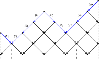
Figure 3. The lattice diagram of $L_{\{1,5,6\}}$ in ${\rm CM}(B_{3,9})$ with its rim (blue arrows, with labels $x_{1},y_{2},y_{3},y_{4},x_{5},x_{6},y_{7},y_{8},y_{9}$).

The upper boundary of the lattice diagram of $L_{I}$ is called the rim of $L_{I}$ (we usually omit the arrows when drawing the rim). The $k$ subset $I\subset[n]$ of the rank $1$ module $L_{I}$ can be read off as the set of labels on the edges going down to the right which are on the rim of $L_{I}$, i.e., the labels of the $x_{i}$’s appearing in the rim. For simplicity, we usually do not draw the labels of the rim in the figures.

We recall the notion of peaks and valleys of rank 1 modules from [4].

Definition 2.4.

If $I$ is a $k$-subset of $[n]$, the set of peaks of $L_{I}$ is the set $\{i\mid i\notin I,i+1\in I\}$. The set of valleys of $L_{I}$ is $\{i\mid i\in I,i+1\notin I\}$.

The rank 1 modules can be viewed as building blocks for the category as every module in ${\rm CM}(B_{k,n})$ has a filtration with factors which are rank $1$ modules (cf. [16, Proposition 6.6]). Let $M$ be a rank $m$ module in ${\rm CM}(B_{k,n})$ with factors $L_{I_{1}},\dots,L_{I_{m}}$ in its generic filtration, where $L_{I_{m}}$ is a submodule of $M$. We write $M=L_{I_{1}}|L_{I_{2}}|\cdots|L_{I_{m}}$ or $M=\small\begin{array}[]{c}L_{I_{1}}\\ \hline\cr\vdots\\ \hline\cr L_{I_{m}}\end{array}$ . The ordered collection of $k$-subsets $I_{1},\ldots,I_{m}$ in the generic filtration of $M$ is called the profile of $M$, denoted $P_{M}$. We write $P_{M}=\small\begin{array}[]{c}I_{1}\\ \hline\cr\vdots\\ \hline\cr I_{m}\end{array}$ or $P_{M}=I_{1}|\cdots|I_{m}$ if $M$ has a filtration having factors $L_{I_{1}},\ldots,L_{I_{m}}$ (in this order). We sometimes write $M=P_{M}$ to indicate that $M$ is a module with profile $P_{M}$. Note that in general, such a filtration is not unique, but in case $M$ is rigid, the filtration is unique in the sense that it gives a canonical ordered set of rank 1 composition factors (see next subsection, [16, Definition 6.4], and [16, Proposition 6.6] for more details on the uniqueness of the profile of the Cohen-Macaulay modules which are given as subspace configurations).

2.2. Subspace configurations

Here, we follow the set-up of [16, Section 6]. Let $M$ be a module in ${\rm CM}(B_{k,n})$ and consider a filtration of $M$. We draw the lattice diagrams of all the rank 1 modules appearing in the filtration, in the filtration order. The rims of the filtration factors in this picture, together with the multiplicities of the elements in the monimial bases are called the set of contours of $M$. For indecomposable modules, contours are close-packed in the sense that there can be no “walk” (unoriented path) going around between two layers of the contours of $M$. The result is a lattice diagram where the multiplicities of the elements of the monomial basis are equal to the rank of $M$ below the lowest contour and equal to 1 between the top two contours. For the representation $M$, connected regions with constant multiplicity in the lattice diagram correspond to isomorphic vector spaces, e.g., we can consider the region below the lowest contour to be $\mathbb{C}^{\operatorname{rank}\nolimits M}$. This view-point gives a subspace configuration associated with $M$, drawn as a poset, with the convention that an edge $i\--j$ with $i<j$ denotes an inclusion of an $i$-dimensional space into a $j$-dimensional space. With slight abuse of notation, we also call the poset of a subspace configuration a subspace configuration. The poset (or subspace configuration) is a graph where the labels on the vertices are viewed as multiplicities, they are elements of $\{1,2,\dots,\operatorname{rank}\nolimits M\}$, the multiplicity $\operatorname{rank}\nolimits M$ only appears in one vertex.

The poset can thus be viewed as a representation for the underlying graph, with the orientations on the edges coming from the inclusions in $M$, i.e., pointing from the smaller to the larger numbers.

Example 2.5.

Let $M$ be a module in ${\rm CM}(B_{3,9})$ with profile $169\mid 147\mid 358$. Figure 4 (A) shows the contours of $M$. In (A), below the first rim, every region has an upper boundary which is a part of the rim of the quotient $M$ by the rank 1 modules above it. In (B), we show the poset of the subspace configuration of $M$. This graph can be simplified to (C) as we explain below.

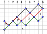
(a)

(b)

(c)

Figure 4. The subspace configuration (B) corresponds to the graph of contours (A). The subspace configuration (B) simplifies to (C).

The following lemma follows from the discussion below Definition 6.4 in [16].

Lemma 2.6.

If $M$ is indecomposable, then the subspace configuration is indecomposable, i.e., the poset diagram is an indecomposable representation for the oriented poset graph.

Using this, we get that if the poset diagram is a direct sum of two non-zero representations for the poset graph, it induces a direct sum decomposition of $M$ in ${\rm CM}(B_{k,n})$.

To see whether the subspace configuration is indecomposable, it is convenient to simplify the poset diagrams.

The poset diagrams of subspace configurations can be simplified as follows. A subspace can be identified as the intersection of several subspaces it maps into and may be omitted: for example, in Figure 4 (B), each of the 1-dimensional subspaces has to map in two different 2-dimensional subspaces of the 3-dimensional space at the bottom. In each case, these two different 2-dimensional subspaces intersect in a subspace of dimension 1. Hence this 1-dimensional subspace mapping into them is already determined and can be omitted from the diagram.

If after applying simplifications, the underlying graph of the poset is the graph of a Dynkin diagram, we know that if the poset diagram is indecomposable, it has to be a positive root for it.

Under the above rules, the subspace configuration in Figure 4 (B) from Example 2.5 simplifies to (C). This is of Dynkin type $D_{4}$ and the simplified poset is not a root for $D_{4}$, hence the poset diagram is not indecomposable.

2.3. Auslander-Reiten translations and shifts

By the symmetry of the algebra $B_{k,n}$, adding a fixed number to every element in every $k$-subset of the profile of a module and changing the linear maps in the representation accordingly preserves indecomposability and rigidness.

Definition 2.7.

Let $M$ and $M^{\prime}$ be indecomposable modules in ${\rm CM}(B_{k,n})$, with profiles $P$ and $P^{\prime}$. If there is a number $a\in[n]$ such that $P^{\prime}$ is obtained by adding $a$ to each entry of $P$ (reducing modulo $n$), we say that $M^{\prime}$ is a shift of $M$ by $a$ and that the profile $P^{\prime}$ is a shift of $P$ (by $a$).

Lemma 2.8.

Let $M$ and $M^{\prime}\in{\rm CM}(B_{k,n})$ be indecomposable and let $M^{\prime}$ be a shift of $M$. Then $M$ is rigid if and only if $M^{\prime}$ is rigid.

If the Auslander-Reiten translation leaves a module invariant, it cannot be rigid.

Lemma 2.9.

Let $M$ be a module in $\underline{{\rm CM}}(B_{k,n})$. If $\tau^{-1}(M)=M$, then $M$ is non-rigid.

Proof.

If $M=\tau^{-1}(M)$, then there is an almost split sequence

$$M\to E\to M$$

in ${\rm CM}(B_{k,n})$. This sequence does not split, so $M$ is not rigid. ∎

Lemma 2.10.

For any indecomposable module $M$ in $\underline{{\rm CM}}(B_{k,n})$, if the profile of $\tau^{-1}(M)$ is the same as the profile of $M$, then $M$ is non-rigid.

Proof.

Suppose that $\tau^{-1}(M)$ and $M$ have the same profile. If $M$ is rigid, then $\tau^{-1}(M)=M$ since rigid indecomposable modules are uniquely determined by their profiles. By Lemma 2.9 , $M$ is non-rigid. This is a contradiction. Therefore $M$ is non-rigid. ∎

Consider the subcategory ${\rm Sub}\,Q_{k}$ of the module category of the preprojective algebra of type $A_{n-1}$ (on vertices $1,2,\dots,n-1$) consisting of modules with socle concentrated at the vertex $k$. In other words, ${\rm Sub}\,Q_{k}$ is the exact subcategory of modules having injective envelope in the additive hull of the injective at $k$. It has been studied in the work [13] of Geiss-Leclerc-Schröer on the cluster algebra structure for the coordinate ring of the affine open cell in the Grassmannian. There is a triangle equivalence between the stable categories $\underline{{\rm CM}}(B_{k,n})$ and $\underline{{\rm Sub}}\,Q_{k}$, [16, Corollary 4.6].

Proposition 2.11.

Let $\Gamma$ be the Auslander–Reiten quiver of $\underline{{\rm CM}}(B_{k,n})$ and let $C$ be a component of $\Gamma$. Then

• $\Gamma=C=\mathbb{Z}\Delta/G$ where $\Delta$ is a Dynkin quiver and $G$ is an automorphism group of $\mathbb{Z}\Delta$ in the finite cases $(2,n),(3,6),(3,7)$ and $(3,8)$.

• each $C$ is of the form $\mathbb{Z}A_{\infty}/G_{\lambda}$, where each $G_{\lambda}$ is a power of $\tau$, in the infinite cases.

Proof.

Let $C$ be a connected component of $\Gamma$. The category ${\underline{\rm CM}}(B_{k,n})$ is periodic under $\tau$ by [5, Section 3]. So the triangle equivalent category $\underline{{\rm Sub}}(Q_{k})$ is periodic under $\tau$. We also write $C$ for the connected component of the Auslander-Reiten component of $\underline{{\rm Sub}}(Q_{k})$ corresponding to $C$. We can apply Liu’s result [21, Theorem 5.5], since $\underline{{\rm Sub}}(Q_{k})$ is a Krull–Schmidt and Hom-finite $k$-category, to deduce that $C$ is of the form $\mathbb{Z}\Delta/H$ where $H$ is an automorphism group of $\mathbb{Z}\Delta$ containing a power of the translation $\tau$ or $C$ is a stable tube, i.e., isomorphic to $\mathbb{Z}A_{\infty}/\tau^{m}$ for some $m>0$.

Let $T$ be a cluster-tilting object in the stable category ${\underline{\rm CM}}(B_{k,n})$ (for example, as given in [7, Section 3], without the projective summands). Let $A$ be its endomorphism algebra. If the Auslander–Reiten quiver of ${\rm mod}\,A$ contains a finite connected component, then this is the only component and ${\rm mod}\,A$ is representation finite by [1, Theorem IV.5.4]. Then by [20, Section 2.1] we have the following equivalence ${\rm mod}\,A\simeq{\underline{\rm CM}}(B_{k,n})/(T)$ and hence $C$ is as claimed.

If ${\rm mod}\,A$ does not have a finite component, $C$ has to be a tube by the above-mentioned result by Liu. ∎

For further results on $\tau$ periodicity in these categories the reader is referred to [10] and [19]. From the previous proposition it follows that in the infinite cases each Auslander–Reiten sequence has a middle term with at most two indecomposable summands.

We point out that while the Auslander–Reiten components for ${\rm CM}(B_{k,n})$ of infinite type are always tubes, outside of the tame cases, there are many morphisms (those in the radical infinite) connecting the tubes. In these cases it is not true that the indecomposable rigid objects are precisely those sitting in the tubes at a level lower than the rank of the tube.

2.4. A root system for the Grassmannian

Recall the graph $J_{k,n}$ with vertices $1,2,\dots,n-1$ on a line and an additional vertex $n$ attached to the vertex $k$, see Figure 1, as introduced in [16] in the study of ${\rm CM}(B_{k,n})$. This graph gives rise to a Kac-Moody root system (we also call this root system $J_{k,n}$). It is of Dynkin type $D_{n}$ for $k=2$ and of Dynkin type $E_{6},E_{7}$, and $E_{8}$, respectively, for $k=3$ and $n=6,7,$ and $8$, respectively. The root lattice of the Kac-Moody algebra of $J_{k,n}$ can be identified with the lattice $\mathbb{Z}^{n}(k):=\{x=(x_{i})\in\mathbb{Z}^{n}\mid\mbox{ $k$ divides }\sum_{i}x_{i}\}$. We equip this with the inner product

(2.1) $$(x,y)=\sum_{i=1}^{n}x_{i}y_{i}+\frac{2-k}{k^{2}}(\sum_{i=1}^{n}x_{i})(\sum_{i=1}^{n}y_{i})$$

and with the quadratic form $q(x):=(x,x)=\sum_{i=1}^{n}x_{i}^{2}+\frac{2-k}{k^{2}}(\sum_{i=1}^{n}x_{i})^{2}$. The roots of this root system satisfy $q(x)\leq 2$, among them, real roots have $q(x)=2$ and imaginary ones have $q(x)<2$.

Let $e_{1},\dots,e_{n}$ be the standard basis vector of $\mathbb{R}^{n}$. Define $\alpha_{i}=-e_{i}+e_{i+1}$ for $i\in[n-1]$ and $\beta=e_{1}+e_{2}+\dots+e_{k}$. Then the set $\{\alpha_{1},\dots,\alpha_{n-1},\beta\}$ is a system of simple roots for the root system $J_{k,n}$. It will also be convenient to use $\alpha_{n}$ for $\beta$ and we switch freely between the two. The inner products of the simple roots are all equal to $2$ and

$$(\alpha_{i},\alpha_{j})=\begin{cases}-1,&\text{if }|i-j|=1,\\ 0,&\text{otherwise,}\end{cases}\qquad(\beta,\alpha_{i})=\begin{cases}-1,&\text{if }i=k,\\ 0,&\text{otherwise}.\end{cases}$$

Denote by $s_{\alpha}$ the reflection about the hyperplane perpendicular to a root $\alpha$ of $J_{k,n}$ and we write $s_{i}=s_{\alpha_{i}}$ with $i\in[n-1]$ and $s_{\beta}=s_{\alpha_{n}}$. For any root $\alpha$ of $J_{k,n}$ and $v\in\mathbb{R}^{n}$, $s_{\alpha}(v)=v-2\frac{(v,\alpha)}{(\alpha,\alpha)}\alpha$. It is customary to abbreviate the scalar in front of $\alpha$ and to write $\langle v,\alpha^{\vee}\rangle:=2\frac{(v,\alpha)}{(\alpha,\alpha)}$ as we will do later. The Weyl group $W$ of $J_{k,n}$ is the group generated by the simple reflections.

In Section 2 in [16], there is a basis $e_{1},\ldots,e_{n}$ of $\mathbb{Z}^{n}$ such that $\alpha_{i}=e_{i+1}-e_{i}$, $i\in[n-1]$, and $\beta=e_{1}+\ldots+e_{k}$. We write an element $x=\sum_{i=1}^{n}x_{i}e_{i}$ in $\mathbb{Z}^{n}$ as $x=(x_{1},\ldots,x_{n})$.

Lemma 2.12.

For $i\in[n-1]$, $x=(x_{1},\ldots,x_{n})=\sum_{i=1}^{n}x_{i}e_{i}\in\mathbb{Z}^{n}$, we have that $s_{i}(x)$ is obtained from $x$ by interchanging $x_{i}$ and $x_{i+1}$, and $s_{n}(x)=(x_{1}+r,\ldots,x_{k}+r,x_{k+1},\ldots,x_{n}$, where $r=x_{k+1}+\ldots+x_{n}-2\frac{1}{k}\sum_{i=1}^{n}x_{i}$.

Proof.

For $i\in[n-1]$, by (2.1), we have that

$$s_{i}(\sum_{j=1}^{n}x_{j}e_{j}) =\sum_{j=1}^{n}x_{j}e_{j}-2\frac{(\sum_{j=1}^{n}x_{j}e_{j},\alpha_{i})}{(\alpha_{i},\alpha_{i})}\alpha_{i}$$

$$=\sum_{j=1}^{n}x_{j}e_{j}-(x_{i+1}-x_{i})(e_{i+1}-e_{i})=\sum_{j\in[n]\setminus\{i,i+1\}}x_{j}e_{j}+x_{i+1}e_{i}+x_{i}e_{i+1}.$$

Therefore $s_{i}(x)$ is obtained from $x$ by interchanging $x_{i}$ and $x_{i+1}$. Similarly, by (2.1),

$$s_{n}(x_{1},\ldots,x_{n}) =\sum_{j=1}^{n}x_{j}e_{j}-2\frac{(\sum_{j=1}^{n}x_{j}e_{j},\alpha_{n})}{(\alpha_{n},\alpha_{n})}\alpha_{n}$$

$$=\sum_{j=1}^{n}x_{j}e_{j}-\left(\sum_{i=1}^{k}x_{i}+\frac{2-k}{k^{2}}\cdot(\sum_{i=1}^{n}x_{i})\cdot k\right)(e_{1}+\ldots+e_{k})$$

$$=(x_{1}+r,\ldots,x_{k}+r,x_{k+1},\ldots,x_{n}),$$

where $r=x_{k+1}+\ldots+x_{n}-2\frac{1}{k}\sum_{i=1}^{n}x_{i}$. ∎

Jensen, King and Su define in [16, Sections 2,8] a map from the modules of ${\rm CM}(B_{k,n})$ to the root lattice of $J_{k,n}$ by associating a module with its class in the Grothendieck group of ${\rm CM}(B_{k,n})$ (the Grothendieck group is identified with the root lattice of $J_{k,n}$). This works as follows. Let $M$ be a module and $P=P_{M}$ its profile. For $i=1,\dots,n$, let $x_{i}$ be the multiplicity of $i$ in the union of the $k$-subsets in the profile $P$. Then let $x(M)=x(P_{M})=(x_{1},x_{2},\dots,x_{n})\in\mathbb{Z}^{n}$ be the vector of the multiplicities. By definition, $k\mid\sum_{i}x_{i}$, so $x(M)\in\mathbb{Z}^{n}(k)$ and there is an element in $\text{Span}_{\mathbb{R}}\{\beta,\alpha_{1},\ldots,\alpha_{n-1}\}$ corresponding to $x(M)$. We denote this element by $\varphi(M)$ and define $x(\varphi(M))=x(M)$. We say that $M\in{\rm CM}(B_{k,n})$ corresponds to a real (respectively, imaginary) root if $\varphi(M)$ is a real (respectively, imaginary) root of $J_{k,n}$. This terminology is motivated by the fact that in the finite types, all indecomposable modules map to roots and by our results on indecomposable rank 2 and rank 3 modules.

Example 2.13.

Let $M$ be a module in ${\rm CM}(B_{3,9})$ whose profile is $P_{M}=\small\begin{array}[]{c}359\\ \hline\cr 258\\ \hline\cr 147\\ \hline\cr 146\end{array}$. Then $x(M)=(2,1,1,2,2,1,1,1,1)$, $q(M)=2$, and $\varphi(M)=4\beta+2\alpha_{1}+5\alpha_{2}+8\alpha_{3}+6\alpha_{4}+4\alpha_{5}+3\alpha_{6}+2\alpha_{7}+\alpha_{8}$.

3. Canonical profiles and interlacing property

Modules in ${\rm CM}(B_{k,n})$ corresponding to real roots are closely related to canonical profiles which we will discuss in this section. In particular, we will prove that a weakly column decreasing profile is canonical if and only if any two rows of the profile are interlacing.

Definition 3.1.

We say that two sets $J_{1},J_{2}$ of integers are $r$-interlacing if $|J_{1}\backslash J_{2}|=|J_{2}\backslash J_{1}|=r$ and $J_{1}\backslash J_{2}=\{a_{1},a_{2},\ldots,a_{r}\}$, $J_{2}\backslash J_{1}=\{b_{1},b_{2},\ldots,b_{r}\}$, $a_{i}<a_{i+1}$, $b_{i}<b_{i+1}$, $i\in[r-1]$, either $a_{1}<b_{1}<a_{2}<b_{2}<\cdots<b_{r-1}<a_{r}<b_{r}$ or $b_{1}<a_{1}<b_{2}<a_{2}<\ldots<a_{r-1}<b_{r}<a_{r}$. In particular, if $J_{1}=J_{2}$, the sets are $0$-interlacing. We call $J_{1},J_{2}$ interlacing if they are $i$-interlacing for some $i\in\mathbb{Z}_{\geq 0}$.

A profile $P\in\mathcal{P}_{k,n}$ with $k$-subsets $J_{1},\dots,J_{m}$ is called interlacing if for any $i\neq j$, $J_{i}$ and $J_{j}$ are interlacing.

The profile $P_{M}$ from Example 2.13 is interlacing, e.g., the first row and the second row of $P_{M}$ are $2$-interlacing, the third row and the fourth row of $P_{M}$ are $1$-interlacing.

Remark 3.2.

The definition of $i$-interlacing we use in this paper is called tightly $i$-interlacing in [5].

Remark 3.3.

Observe that there are profiles where any two successive rows and the first and the last row are interlacing but where the profile is not interlacing. An example is the profile $\small\begin{array}[]{c}1\hskip 5.69046pt8\ 15\ 20\\ \hline\cr 2\ 11\ 18\ 23\\ \hline\cr 5\ 17\ 21\ 30\\ \hline\cr 4\ 13\ 19\ 29\end{array}$ where rows 1 and 3 are not interlacing.

Recall from the introduction that if $P\in\mathcal{P}_{k,n}$ is a profile with $m$ rows, we write $P=(P_{ij})$, $1\leq i\leq m$, $1\leq j\leq k$, for the profile $P$ with all rows written in increasing order.

Definition 3.4.

Let $P$ be a profile in $\mathcal{P}_{k,n}$ with $m$ rows.

1. $P$ is called weakly column decreasing if for every $j\in[k]$ and for every $i\in[m-1]$, we have $P_{i,j}\geq P_{i+1,j}$.

2. $P$ is called canonical, if it is weakly column decreasing and if for all $j\in[2,k]$, $P_{m,j}\geq P_{1,j-1}$.

3. If $P$ is canonical and $q(P)=2$, we say it is real. We write $C_{k,n}^{\rm re}\subset\mathcal{P}_{k,n}$ for the set of all canonical profiles $P$ with $q(P)=2$.

Example 3.5.

The profile $P=\small\begin{aligned} 359\\ \hline\cr\\[-9.0pt] 258\\ \hline\cr\\[-9.0pt] 147\\ \hline\cr\\[-9.0pt] 146\end{aligned}$ of $\mathcal{P}_{3,9}$ is canonical and $P\in C_{3,9}^{\rm re}$.

Definition 3.6.

Let $P$ be a profile in ${\mathcal{P}}_{k,n}$ with $m$ rows. Then a profile $P^{\prime}$ is a cyclic permutation of $P$ if $P^{\prime}$ is obtained by cyclically permuting the rows of $P$.

Proposition 3.7.

Let $P\in\mathcal{P}_{k,n}$ be a weakly column decreasing profile. Then $P$ is canonical if and only if any two rows of $P$ are interlacing.

Proof.

For $m=1$ there is nothing to show. So assume $m\geq 2$.
($\Rightarrow$) Suppose that $P$ is canonical and $P$ has two or more rows. Write $P=(P_{ij})_{1\leq i\leq m,1\leq j\leq k}$, $P_{ij}<P_{i,j+1}$, $i\in[m]$, $j\in[k-1]$. Consider any two rows

$$\begin{array}[]{ccc}P_{i_{1},1}&\cdots&P_{i_{1},k}\\ P_{i_{2},1}&\cdots&P_{i_{2},k}\end{array}$$

with $i_{1}<i_{2}$. Let $I_{i}:=\{P_{i_{j},1},\ldots,P_{i_{j},k}\}$ for $j=1,2$. These are both $k$-subsets of $[n]$ as $P$ is a profile. Note that $|I_{2}\setminus I_{1}|=|I_{1}\setminus I_{2}|=:\ell$ for some $\ell\geq 0$.

To check the interlacing property, we consider $\widetilde{I_{i}}:=I_{i}\setminus(I_{1}\cap I_{2})$ for $i=1,2$. So we can write $\widetilde{I_{1}}=\{P_{i_{1},j_{1}},P_{i_{1},j_{2}},\dots,P_{i_{1},j_{\ell}}\}$ and $\widetilde{I_{2}}=\{P_{i_{2},j_{1}^{\prime}},P_{i_{2},j_{2}^{\prime}},\dots,P_{i_{2},j_{\ell}^{\prime}}\}$ for $1\leq j_{1}<j_{2}<\dots<j_{\ell}\leq k$ and $1\leq j_{1}^{\prime}<j_{2}^{\prime}<\dots<j_{\ell}^{\prime}\leq k$. Since $P$ is canonical, $j_{r}^{\prime}\leq j_{r}$ for $r=1,\dots,\ell$ and $j_{r}<j^{\prime}_{r+1}$ for $r=1,\dots,\ell-1$.

The $\ell$-subsets $\widetilde{I_{1}}$ and $\widetilde{I_{2}}$ are disjoint subsets by construction. We need to see that they are $\ell$-interlacing, i.e., that $P_{i_{2},j_{1}^{\prime}}<P_{i_{1},j_{1}}<P_{i_{2},j_{2}^{\prime}}<\dots<P_{i_{1},j_{\ell}}$.

In case $j_{r}^{\prime}=j_{r}$, we have $P_{i_{2},j_{r}^{\prime}}\leq P_{i_{1},j_{r}}$ by the weakly column decreasing condition and $P_{i_{1},j_{r}}\leq P_{i_{2},j^{\prime}_{r+1}}$ since $P$ is canonical. And since $\widetilde{I_{1}}$ and $\widetilde{I_{2}}$ are disjoint, both inequalities have to be strict.

So assume that $j_{r}^{\prime}<j_{r}$. Then $P_{i_{1},j_{r}^{\prime}}<P_{i_{1},j_{r}}$. By the weakly column decreasing condition, we have $P_{i_{2},j_{r}^{\prime}}\leq P_{i_{1},j_{r}^{\prime}}$. Therefore $P_{i_{2},j_{r}^{\prime}}<P_{i_{1},j_{r}}$. Furthermore, $P_{i_{1},j_{r}}\leq P_{i_{2},j_{r+1}^{\prime}}$ as $P$ is canonical and so, since $\widetilde{I_{1}}$ and $\widetilde{I_{2}}$ are disjoint, we have $P_{i_{1},j_{r}}<P_{i_{2},j_{r+1}^{\prime}}$.

($\Leftarrow$) Let $P\in\mathcal{P}_{k,n}$ with $m\geq 2$ rows. Write $P=(P_{ij})_{1\leq i\leq m,1\leq j\leq k}$, $P_{ij}<P_{i,j+1}$, $i\in[m]$, $j\in[k-1]$. For some $1\leq j<k$, consider the four elements in rows $1$ and $m$ of $P$ and in the two successive columns $j,j+1$:

$$\begin{array}[]{cc}P_{1,j}&P_{1,j+1}\\ &\\ P_{m,j}&P_{m,j+1}.\end{array}$$

We have to show that $P_{1,j}\leq P_{m,j+1}$. Denote by $I_{1},I_{m}$ the $k$-subsets of the first and last row respectively.

a) If $P_{1,j}=P_{m,j}$, then we have $P_{1,j}<P_{m,j+1}$ since $P_{1,j}=P_{m,j}<P_{m,j+1}$.

b) Let $P_{1,j+1}=P_{m,j+1}$. Then $P_{1,j}<P_{m,j+1}$ as $P_{m,j+1}=P_{1,j+1}>P_{1,j}$.

So we have to consider the cases where $P_{1,j}\neq P_{mj}$ and $P_{1,j+1}\neq P_{m,j+1}$. Since $P$ is weakly column decreasing, this means that $P_{1,j}>P_{m,j}$ and $P_{1,j+1}>P_{m,j+1}$.

c) Let $P_{1,j}>P_{m,j}$ and $P_{1,j+1}>P_{m,j+1}$. Suppose that $P_{1,j}>P_{m,j+1}$. If $j=1$, then the first row and the last row are not interlacing. This is a contradiction. Therefore $j>1$. Now we have a set $\{P_{m,j},P_{m,j+1}\}$ in which every element is smaller than $P_{1,j}$. We define this set $\{P_{m,j},P_{m,j+1}\}$ to be the active set and the element $P_{1,j}$ the active maximum. We now check the elements $P_{1,j-1},P_{1,j-2},\ldots,P_{1,1}$ one by one as follows: we compare each of these elements with the smallest element in the active set and with further elements of row $m$. Denote the minimum in the active set by $A$. In the beginning, we have $A=P_{m,j}$.

• If $P_{1,j-1}<A$ and $P_{1,j-1}\neq P_{m,j-1}$, then the elements in the active set $\{P_{m,j},P_{m,j+1}\}$ lie between two consecutive numbers $P_{1,j-1},P_{1,j}$ in $I_{1}\setminus I_{m}$. This contradicts the assumption that the first and the last row are interlacing.

• If $P_{1,j-1}<A$ and $P_{1,j-1}=P_{m,j-1}$, we keep the active set and the active maximum and continue with $P_{1,j-2}$.

• If $P_{1,j-1}=A$, then we have $P_{m,j-1}<A=P_{1,j-1}$. We replace the active set by removing $A$ and adding $P_{m,j-1}$. As $P_{1,j}$ is still larger than the elements of the new active set, we keep the active maximum. We then continue with $P_{1,j-2}$.

• If $P_{1,j-1}>A$ and $P_{1,j-1}\not\in I_{1}\cap I_{m}$, then $P_{m,j-1}<P_{m,j}=A<P_{1,j-1}$. We replace the active set by $\{P_{m,j-1},P_{m,j}\}=\{P_{m,j-1},A\}$ and replace the active maximum by $P_{1,j-1}$. We then continue with $P_{1,j-2}$.

• If $P_{1,j-1}>A$ and $P_{1,j-1}\in I_{1}\cap I_{m}$, then $P_{m,j-1}<P_{m,j}=A<P_{1,j-1}<P_{1,j}$. We change the active set by removing $P_{1,j-1}$ (if it is contained in it - otherwise we do not remove anything from the active set) and by adding $P_{m,j-1}$. We keep the active maximum and continue with $P_{1,j-2}$.

Continuing this procedure, the active set always has two or more elements. By construction, every element in the active set is smaller than the active maximum. We have one of the following situations which both contradict the assumption that $I_{1},I_{m}$ are interlacing:

• At some step, the elements in the active set lie between two consecutive elements in $I_{1}\setminus I_{m}$.

• In the last step, after we check $P_{1,1}$, the elements in the active set are smaller than the active maximum element and this active maximum is the smallest element in $I_{1}\setminus I_{m}$.

We thus get $P_{1,j}\leq P_{m,j+1}$ as claimed. ∎

4. Rank 2 rigid indecomposable modules in ${\rm CM}(B_{k,n})$

In this section, we give a lower bound for the number of indecomposable modules of rank $2$ corresponding to roots in ${\rm CM}(B_{k,n})$.

By [5, Section 5], every rank $2$ indecomposable module in ${\rm CM}(B_{k,n})$ corresponding to a real root is of the form $L_{I}\mid L_{J}$ where $I$ and $J$ are 3-interlacing. From that we can deduce that there are at most $2{n\choose 6}{n-6\choose k-3}$ such rigid modules (as they come in pairs).

Recall from Subsection 2.2 that we can draw modules as lattice diagrams or as collections of rims, as in Figure 4. For simplicity, we often do not write the numbers (the dimensions of the vector spaces) in the regions of the lattice diagrams.

By abuse of notation, we will call a profile or the lattice diagram of a rank $m$ module a profile of rank $m$ or a lattice diagram of rank $m$.

Consider a lattice diagram of rank 2: it has two rims which may meet several times (in particular, they will do so if the module is indecomposable). Similarly, if we consider a lattice diagram of higher rank, any two successive rims may meet several times.

Definition 4.1.

Consider a rank $m$ module with filtration $L_{I_{1}}\mid L_{I_{2}}\mid\dots\mid L_{I_{m}}$. Let $R_{1}$ and $R_{2}$ be the rims of $L_{I_{j}}$ and $L_{I_{j+1}}$ for some $1\leq j<m$.

We call the non-empty regions formed by the two rims, between any two successive meeting points (reducing modulo $n$, if necessary) the quasi-boxes between the two rims. In particular, we say that $R_{1}$ and $R_{2}$ form $n$ quasi-boxes if there are $n$ quasi-boxes between them. If a quasi-box is of rectangular shape, we call it a box.

We define the size (or right-size) of a (quasi-)box to be the sum of the sizes of the intervals in the part of $I_{j}$ corresponding to this box.

The co-size (or left-size) of a quasi-box is the sum of the sizes of the intervals of $I_{j}^{c}$ corresponding to this box.

Example 4.2.

Figure 5 shows an example for $(k,n)=(7,16)$. The $7$-subsets forming the rims are $I=\{4,5,8,10,13,14,16\}$ and $J=\{1,2,6,7,11,13,15\}$. There are four quasi-boxes, two of them are boxes. To illustrate size and co-size: The quasi-box between branching points $5$ and $10$ has size 2 and co-size 3, the quasi-box between branching points $10$ and $14$ has size 2 and co-size 2.

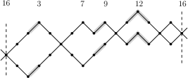
Figure 5. Two rims formed by $7$-subsets of $n=16$, with branching points $\{5,10,14,16\}$. Parallel segments are indicated by the shading.

The map from indecomposable modules to elements of the root system does not depend on the order of the factors in the filtration, it only depends on the elements of the $k$-subsets in its profile. We thus give this set a name. Let $P$ be the profile of an indecomposable module. The content of $P$, ${\rm con}(P)$, is the multiset consisting of the elements of all $k$-subsets in $P$, for example,

$${\rm con}\left(\small\begin{aligned} 147\\ \hline\cr\\[-9.0pt] 258\\ \hline\cr\\[-9.0pt] 358\\ \hline\cr\\[-9.0pt] 369\end{aligned}\right)=\{1,2,3,3,4,5,5,6,7,8,8,9\}.$$

If we have a rank 2 module $M=L_{I}\mid L_{J}$, adding a constant number to all entries in the involved $k$-subsets keeps some properties of the module (e.g., indecomposabilty, rigidness) but changes others, e.g., the content of $P_{M}$ (i.e., the labels appearing in $I\cup J$) will change in general.

We introduce operations on the profiles. The “collapse” operation removes parallel lines from profiles and the $a$-shift preserves the content as we will need to study different indecomposable modules which give rise to the same root.

Definition 4.3.

(Collapsing profiles and profile $a$-shift)

1. Let $P=I_{1}\mid I_{2}$ be a rank 2 profile in $\mathcal{P}_{k,n}$. Let $n^{\prime}=n-|I_{1}^{c}\cap I_{2}^{c}|-|I_{1}\cap I_{2}|$ and $\psi:[n]\setminus((I_{1}^{c}\cap I_{2}^{c})\cup(I_{1}\cap I_{2}))\to[n^{\prime}]$ be the bijection respecting the order on these sets. We say that $\psi(I_{1})\mid\psi(I_{2})$ is the collapse of $I_{1}\mid I_{2}$.

2. Let $P=I_{1}\mid I_{2}\in\mathcal{P}_{k,n}$ be a rank 2 profile and $a\in[n]$. For $j=1,2$, define $I_{j}^{\prime}$ as the set $\psi^{-1}(\psi(I_{j})+a\pmod{n^{\prime}})\cup(I_{1}\cap I_{2})$. Then $P^{\prime}=I^{\prime}_{1}\mid I^{\prime}_{2}$ is called the $a$-shift of $P$.

Observe that the elements of $I_{1}\cap I_{2}$ and the elements of $I_{1}^{c}\cap I_{2}^{c}$ are fixed under an $a$-shift for any $a\in[n]$. So for elements in $I_{1}\cap I_{2}$, the $a$-shift does not do anything whereas the elements in only one of the $k$-subsets might get moved to the other.

Figure 6. The collapse of the profile $I_{1}\mid I_{2}$ from Figure 5.

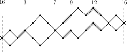
Figure 7. The 2-shift of the profile from Figure 5

Example 4.4.

Let $P=I_{1}\mid I_{2}$ with $I_{1}=\{4,5,8,10,13,14,16\}$ and $I_{2}=\{1,2,6,7,11,13,15\}$. The collapse of $I_{1}\mid I_{2}$ is $\{3,4,7,8,10,12\}\mid\{1,2,5,6,9,11\}$, see Figure 6. The $2$-shift $I_{1}\mid I_{2}$ is the profile $\{2,6,7,11,13,14,16\}\mid\{1,4,5,8,10,13,15\}$ it is shown in Figure 7.

The following is immediate from the definition of $a$-shifts.

Lemma 4.5.

Let $P$ be a rank $2$ profile in $\mathcal{P}_{k,n}$ and let $P^{\prime}$ be an $a$-shift of $P$. Then ${\rm con}(P^{\prime})={\rm con}(P)$. In particular, the root of $P$ is the same as the root of $P^{\prime}$. Furthermore, if the $k$-subsets of $P$ are $r$-interlacing, then the $k$-subsets of $P^{\prime}$ are also $r$-interlacing.

Recall that we always assume $k\leq n/2$.

Lemma 4.6.

Let $M$ be indecomposable of rank $2$ module in ${\rm CM}(B_{k,n})$ and assume that $M$ has a filtration $L_{I}\mid L_{J}$. Then the rims of $L_{I}$ and $L_{J}$ form at least three quasi-boxes. Furthermore, $q(M)\in\{2,0,-2,\ldots,8-2k\}$ and $\varphi(M)$ is a root of $J_{k,n}$.

Proof.

That the two rims have to form at least three quasi-boxes for indecomposability follows from the subspace configurations (cf. Remark 3.2 in [5]). Let $l$ be the number of quasi-boxes.

Let $x(M)=x(P_{M})=(x_{1},\dots,x_{n})$ be the vector of the multiplicities (Section 2.4).

Since $M$ has rank 2, the sum $\sum_{i=1}^{n}x_{i}$ is equal to $2k$ and $0\leq x_{i}\leq 2$ for all $i$. Also, since $I$ and $J$ form at least three quasi-boxes, we have $|I\setminus J|=|J\setminus I|\geq 3$ and so the number of $x_{i}$’s which are equal to 2 is at most $k-3$. But then $\sum x_{i}^{2}\leq 4(k-3)+6$.

Denote by $a$ (resp. $b$) the number of $2$’s (resp. $1$’s) in $\{x_{i}:i\in[n]\}$. Note that $b$ is even and $b\geq 6$ since there are at least three quasi-boxes. Then $\sum_{i}x_{i}^{2}=4a+b\leq 4k-6$ and $\sum_{i}x_{i}=2a+b=2k$. Therefore $0\leq a\leq k-3$, $b=2k-2a$. Hence $q(M)=\sum_{i=1}^{n}x_{i}^{2}-4(k-2)\in\{2,0,-2,\ldots,8-2k\}$.

First we consider the case when $q(M)=2$. That is, $a=k-3$ and $b=6$. We denote $x(M)=x(\varphi(M))=x=(x_{1},\ldots,x_{n})$. Up to Weyl group action, we may assume that $x(M)=(2,\ldots,2,1,\ldots,1,0,\ldots,0)$ (see Lemma 2.12), where the number of $2$’s is $k-3$ and the number of $1$’s is $6$. Therefore

$$\varphi(M)=2\beta+\alpha_{k-2}+2\alpha_{k-1}+3\alpha_{k}+2\alpha_{k+1}+\alpha_{k+2}.$$

By Lemma 2.12, we have that $s_{k}s_{k+1}s_{k+2}s_{k-1}s_{k}s_{k+1}s_{k-2}s_{k-1}s_{k}s_{\beta}(\varphi(M))=\beta$ which is a simple root. Therefore $\varphi(M)$ is a real root of $J_{k,n}$ by definition, [17, Section 5.1].

Now we consider the case when $q(M)<2$. That is $a<k-3$ and $b=2k-2a$. Denote by $Q^{+}=\oplus_{i=1}^{n}\mathbb{Z}_{\geq 0}\alpha_{i}$ the positive part of the root lattice of $J_{k,n}$ where we write $\alpha_{n}$ for $\beta$ for the moment. For $\alpha\in Q^{+}$, denote by ${\rm supp}(\alpha)$ the support of $\alpha$, i.e., the subdiagram of $J_{k,n}$ corresponding to the simple roots having non-zero coefficients in $\alpha$. Let $K=\{\alpha\in Q^{+}\backslash\{0\}\mid\langle\alpha,\alpha_{i}^{\vee}\rangle\leq 0,i\in[n]\text{ and ${\rm supp}(\alpha)$ is connected}\}$. By [17, Theorem 5.4], the set of all positive imaginary roots of $J_{k,n}$ is equal to $\cup_{w\in W}w(K)$. Up to Weyl group action, we may assume that $x(M)=(2,\ldots,2,1,\ldots,1,0,\ldots,0)$ (see Lemma 2.12), where the number of $2$’s is $a$ and the number of $1$’s is $b$. Therefore

We have that $\langle\varphi(M),\alpha_{a}^{\vee}\rangle=\langle\varphi(M),\alpha_{a+b}^{\vee}\rangle=-1$, $\langle\varphi(M),\alpha_{i}^{\vee}\rangle=0$ for $i\in[n-1]\setminus\{a,a+b\}$ and $\langle\varphi(M),\beta^{\vee}\rangle=4-(k-a)\leq 0$ since $a<k-3$. Moreover, ${\rm supp}(\varphi(M))$ is connected. Therefore $\varphi(M)$ is an imaginary root. ∎

Note that if $a=0$, $b=2k$ and $q(M)=8-2k$, whereas if $a=k-3$, we have $b=6$ and $q(M)=2$. So when $k=3$, all indecomposable rank 2 modules have $q(M)=2$ and for $k>3$, we can find rank 2 modules with the lower bound $q(M)=8-2k$ by taking two $k$-interlacing subsets.

Theorem 4.7.

Consider rank $2$ modules in ${\rm CM}(B_{k,n})$.
(1) Assume that $M$ has filtration $L_{I}\mid L_{J}$. Then $M$ is rigid indecomposable if the rims of $L_{I}$ and $L_{J}$ form three boxes.
(2) The number of profiles of rigid indecomposable rank $2$ modules in ${\rm CM}(B_{k,n})$ is at least

$$N_{k,n}=\sum_{r=3}^{k}(\frac{2r}{3}\cdot p_{1}(r)+2r\cdot p_{2}(r)+4r\cdot p_{3}(r))\cdot{n\choose 2r}{n-2r\choose k-r},$$

where $p_{i}(r)$ is the number of partitions $r=r_{1}+r_{2}+r_{3}$ such that $r_{1},r_{2},r_{3}\in\mathbb{Z}_{\geq 1}$ and $|\{r_{1},r_{2},r_{3}\}|=i$.

Proof.

Note that there are no indecomposable rank 2 modules for $k<3$ and $N_{k,n}=0$ in this case. So we can assume $k\geq 3$.

To prove part (1), by Corollary A.12, we can assume that $I\cap J=I^{c}\cap J^{c}=\emptyset$ (all parallel segments in the two rims can be removed). By Lemma 4.6, the two rims have to form at least three quasi-boxes for a rank 2 module to be indecomposable.

So assume that $L_{I}$ and $L_{J}$ form exactly three boxes. Since $I\cap J=I^{c}\cap J^{c}=\emptyset$, the syzygy $\Omega(M)$ is a rank 1 module, so $M$ is rigid: the projective cover of $M$ has exactly three summands and so $\Omega(M)=\tau^{-1}(M)$ is a rank 1 module. In particular, $M$ is rigid.

For (2), we have to determine how many profiles with 2 rows exist with exactly three boxes, we claim this to be equal to $N_{k,r}$. To show this, we consider how many different profiles can arise from a given one through $a$-shifts and reordering of boxes. So assume $I$ and $J$ are the two rows of a rank 2 profile (of a rigid indecomposable module). By Corollary A.12, we can assume that $I$ and $J$ are fully reduced, i.e., that $I\cap J=I^{c}\cap J^{c}=\emptyset$.

We have that $|I\cup J|=2r$ for some $r\in[3,k]$. Let $r_{1},r_{2},r_{3}$ be the sizes of the three boxes (ordered such that the box of size $r_{1}$ starts with the smallest $i\in\{1,2\dots,n\}\setminus(I^{c}\cap J^{c})$). If $|\{r_{1},r_{2},r_{3}\}|=1$, then $3\mid r$ and the partial shifts yield $2r/3$ different modules with the same content. If $|\{r_{1},r_{2},r_{3}\}|=2$, the partial shifts yield $2r$ different modules with the same content. If $|\{r_{1},r_{2},r_{3}\}|=3$, the partial shifts yield $2r$ additional different modules with the same content. Reordering the boxes so that the sizes are $r_{1},r_{3},r_{2}$ (i.e., interchanging two boxes) yields $2r$ additional modules with the same content (as the sizes are all different). So $4r$ different modules with the same content.

The claim then follows with part (1), as every such profile with exactly three boxes gives a rigid indecomposable. ∎

Conjecture 4.8.

The number of profiles of rigid indecomposable rank $2$ modules in ${\rm CM}(B_{k,n})$ is $N_{k,n}$.

Note that in the tame cases $(3,9)$ and $(4,8)$, the number of rigid indecomposable rank 2 modules can already be deduced from the results of [5]. In the general infinite case, there are many morphisms between tubes and even though the rank 2 modules are sitting low in their tubes, a priori, the formula of Theorem 4.7 (2) only gives a lower bound.

Example 4.9.

In case $k=4$ and $n=8$, the formula gives

$$N_{4,8}=\sum_{r=3}^{4}(\frac{2r}{3}\cdot p_{1}(r)+2r\cdot p_{2}(r)+4r\cdot p_{3}(r))\cdot{8\choose 2r}{8-2r\choose 4-r},$$

The only possibilities to form three boxes are $r=3$ with $r_{1}=r_{2}=r_{3}=1$ and $r=4$ with $r_{1}=r_{2}=1$, $r_{3}=2$. So $p_{1}(3)=1$, $p_{2}(4)=1$ and all other $p_{i}(r)$ are $0$. The formula gives $N_{4,8}=2p_{1}(3){8\choose 6}{2\choose 1}+8p_{1}(4){8\choose 8}{0\choose 0}$ $=2\cdot 28\cdot 2+8=120$, which is equal to the number of rigid indecomposables in this case, cf. [5, Section 7]. For $r=3$, all these modules correspond to real roots and the 8 modules with imaginary roots arise from $r=4$.

5. Subspace configurations of rank 3 modules

In this section, we use the subspace configurations to derive necessary conditions for indecomposability (Subsection 5.1) and then use these to study the roots associated with indecomposable rank 3 modules (Subsection 5.2). We automatically have $k\geq 3$, as there are no indecomposable higher rank modules for $k\leq 2$. To find these necessary conditions, we consider the number of (quasi-)boxes between the two pairs of successive rims of $M$; the number of valleys of the upper rim is an upper bound for this number.

Note that if a module $M$ is indecomposable, any two successive rims of $M$ are “closely packed” in the sense that there cannot be a walk between the two rims, [16, Section 6].

5.1. Necessary conditions for indecomposability

The first case is when $I=J$, then there are no boxes between the two rims of $L_{I}=L_{J}$.

Lemma 5.1.

Let $M=L_{I}|L_{J}|L_{K}\in{\rm CM}(B_{k,n})$ be indecomposable. If $I=J$, then the rims of $L_{J}$ and $L_{K}$ form at least four quasi-boxes.

Proof.

Suppose that $M=L_{I}|L_{J}|L_{K}\in{\rm CM}(B_{k,n})$ is indecomposable, with $I=J$. In this case, the subspace configuration of $M$ looks like a star. It has one vertex with multiplicity 3 and $m\geq 0$ vertices with $2$, each with an arrow towards $3$. Such a subspace configuration is decomposable for $m\leq 3$. ∎

Let $I$ and $J$ be $k$-subsets. Instead of writing that (quasi-)boxes are formed by the rims of $L_{I}$ and $L_{J}$, we will also say that the (quasi-)boxes are formed by $L_{I}$ and $L_{J}$ or by $I$ and $J$.

Lemma 5.2.

Let $M=L_{I}|L_{J}|L_{K}\in{\rm CM}(B_{k,n})$ be indecomposable.
(1) If $L_{J}$ and $L_{K}$ form up to three quasi-boxes, then $L_{I},L_{J}$ form at least two quasi-boxes or the subspace configuration of $M$ is (G) in Figure 8.
(2) If $L_{I},L_{J}$ form one quasi-box, then $L_{J},L_{K}$ form at least four quasi-boxes or the subspace configuration of $M$ is (G) in Figure 8.

Proof.

Suppose that $M=L_{I}|L_{J}|L_{K}\in{\rm CM}(B_{k,n})$ is indecomposable and $L_{J},L_{K}$ form at most three quasi-boxes. By Lemma 5.1, $I\neq J$, so $L_{I},L_{J}$ form at least one quasi-box. All possible subspace configurations of $M$ when $I$ and $J$ form one quasi-box are in Figure 8. The only indecomposable one among them is (G). This proves (1).

For the same reason, if $L_{I},L_{J}$ form one quasi-box, then $L_{J},L_{K}$ form at least four quasi-boxes or the subspace configuration of $M$ is (G). ∎

(a)

(b)

(c)

(d)

(e)

(f)

(g)

(h)

(i)

(j)

Figure 8. All subspace configurations for $L_{I}|L_{J}|L_{K}$, where $L_{I},L_{J}$ form one quasi-box and $L_{J},L_{K}$ form at most three quasi-boxes.

Lemma 5.3.

Let $M=L_{I}|L_{J}|L_{K}\in{\rm CM}(B_{k,n})$ be indecomposable, and assume that $L_{I}$ and $L_{J}$ form two quasi-boxes. Then $L_{J},L_{K}$ form at least three quasi-boxes or the subspace configuration of $M$ is (K) from Figure 9.

Proof.

Suppose that $M=L_{I}|L_{J}|L_{K}\in{\rm CM}(B_{k,n})$ is indecomposable and that $L_{I},L_{J}$ form two quasi-boxes. Suppose that $L_{J},L_{K}$ form at most two quasi-boxes. All subspace configurations for such $M$ where $L_{J}$ and $L_{K}$ form at most two quasi-boxes are in Figure 9. The only indecomposable one of them is (K). This proves the claim. ∎

(a)

(b)

(c)

(d)

(e)

(f)

(g)

(h)

(i)

(j)

(k)

Figure 9. All possible subspace configurations of $L_{I}|L_{J}|L_{K}$, $L_{I},L_{J}$ form two quasi-boxes and $L_{J},L_{K}$ form at most two quasi-boxes.

5.2. Rank $3$ indecomposable modules in ${\rm CM}(B_{3,n})$

If we restrict to $k=3$, we can say even more about the profile of a rank 3 indecomposable module, as we will show now.

Lemma 5.4.

Suppose that $M=L_{I}|L_{J}|L_{K}\in{\rm CM}(B_{3,n})$ is indecomposable. Then the subspace configuration of $M$ cannot be (G) of Figure 8 or (K) of Figure 9.

Proof.

The subspace configurations (G) of Figure 8 and (K) of Figure 9 both correspond to a partition of a $k$-subset into four non-trivial parts, hence only occur for $k\geq 4$. ∎

Lemma 5.5.

If $M=L_{I}|L_{J}|L_{K}\in{\rm CM}(B_{3,n})$ is indecomposable, $I$ and $J$ are interlacing.

Proof.

Suppose that $M=L_{I}|L_{J}|L_{K}\in{\rm CM}(B_{3,n})$ is indecomposable. Since $k=3$, $J$ and $K$ form at most three quasi-boxes. Suppose that $I$ and $J$ are not interlacing, then they form at most two quasi-boxes (as $k=3$). By Lemma 5.2, $I$ and $J$ then form exactly two quasi-boxes (as the subspace configuration of $M$ cannot be Figure 8 (G) by Lemma 5.4).

Now we use Lemma 5.3 to see that $J$ and $K$ form at least three quasi-boxes (as the subspace configuration cannot be Figure 9 (K) by Lemma 5.4). As $k=3$, $J$ and $K$ form exactly three quasi-boxes.

Since $k=3$, one of the quasi-boxes has size 1 and one has size 2. Since $I$ and $J$ are not interlacing, the quasi-box of size 2 must be a $2\times 2$ square. But then the rim of $L_{J}$ has exactly two valleys, and since the number of valleys is an upper bound for the number of quasi-boxes, $J$ and $K$ cannot form three quasi-boxes. A contradiction. ∎

Theorem 5.6.

Let $M\in{\rm CM}(B_{3,n})$ be indecomposable of rank $3$. Then $q(M)\in\{0,2\}$ and $\varphi(M)$ is a real or imaginary root of $J_{3,n}$.

Proof.

Suppose that $M=L_{I}|L_{J}|L_{K}$ is an indecomposable module of rank $3$ in ${\rm CM}(B_{3,n})$. If $n<8$, there are no indecomposable rank 3 modules. If $n=8$, all indecomposables correspond to real roots, [16]. So let $n\geq 9$. It suffices to show that the content of $M$ consists of $8$ or $9$ different numbers. If this is the case, we get, up to reordering the $x_{i}$, that the vector of multiplicities of $M$ is $x(M)=(2,1,1,1,1,1,1,0,\dots,0)\in\mathbb{Z}^{n}$ in the first case, with $q(M)=2$ and $x(M)=(1,1,1,1,1,1,1,1,1,0,\dots,0)\in\mathbb{Z}^{n}$ in the second case, with $q(M)=0$.

We consider the quasi-boxes formed by the rims. Note that since $k=3$, any two successive rims form at most three quasi-boxes. We go through these cases.

• If $I=J$, $M$ decomposes by Lemma 5.1, a contradiction.

• Suppose next that $I$ and $J$ form one quasi-box. Since $J$ and $K$ form at most three quasi-boxes, Lemma 5.2 tells that the subspace configuration of $M$ is (G) in Figure 8. This is not possible by Lemma 5.4.

• Assume now that $I$ and $J$ form two quasi-boxes. Then using Lemma 5.3 and Lemma 5.4 we find that $J$ and $K$ have to form three quasi-boxes (each of size 1). In particular, they are 3-interlacing, $|J\cup K|=6$ and $J\cap K=\emptyset$.

  By Lemma 5.5, $I$ and $J$ are interlacing and since we have two quasi-boxes, $I$ and $J$ are 2-interlacing. So $|I\cap J|=1$. This implies that $I\cup J\cup K$ has at least 7 different elements.

  If $|I\cup J\cup K|=7$, $I$ and $K$ have one element in common. This implies that in the subspace configuration, there is a 2 mapping into a 3 (from the common element of $I$ and $J$). There is also a 1 mapping into two different 2’s. Using the reduction from Section 2.2, we can remove this 1. The resulting diagram has two vertices with a 2, each with a single edge mapping into the 3. Such a subspace configuration is never indecomposable.

  So we get $|I\cup J\cup K|\geq 8$ as claimed.

• Suppose now that $L_{I},L_{J}$ form three quasi-boxes. In particular, as $k=3$, they are 3-interlacing, $|I\cup J|=6$ and $|I\cap J|=\emptyset$.

  The subspace configurations for the cases where $J$ and $K$ form at most one quasi-box are not indecomposable, see Figure 10. So $J$ and $K$ form at least two quasi-boxes.

  If $|I\cup J\cup K|=6$, we have $K\subset I\cup J$ and since $J$ and $K$ form at least two quasi-boxes, $|J\cap K|\leq 1$. So either $K=I$ or two elements of $K$ are in $I$, one is in $J$. In the first case, the subspace configuration consists of three 1’s included simultaneously in two 2’s. So they can be removed by the reduction of Section 2.2. This leaves three 2’s mapping into one 3, not an indecomposable configuration. In the second case, we have two 1’s mapping simultaneously into two 2’s, they can be removed. The resulting subspace configuration contains two 2’s with a single edge into the 3. Again, this is not indecomposable.

  If $|I\cup J\cup K|=7$, two elements of $K$ are in $I\cup J$. These can be both in $I$ or one in $I$ and one in $J$. If they are both in $I$, we have, as before, two 1’s in the subspace configuration mapping into two 2’s each. Removing them leaves two 2’s, each with only one edge to the 3. This is not an indecomposable subspace configuration.

  If one is in $I$ and one in $J$, we can also reduce two 1’s mapping into two 2’s each and get a subspace configuration which is not indecomposable.

  Therefore $I\cup J\cup K$ has at least $8$ different numbers.

We now prove that $\varphi(M)$ is a real or imaginary root in $J_{k,n}$. We will use a similar method as in the proof of Lemma 4.6.

First we consider the case when $q(M)=2$. Up to Weyl group action, we may assume that $x(M)=(2,1,1,1,1,1,1,1,0,\ldots,0)$. Then

$$\varphi(M)=3\beta+\alpha_{1}+3\alpha_{2}+5\alpha_{3}+4\alpha_{4}+3\alpha_{5}+2\alpha_{6}+\alpha_{7}.$$

We have that

$$s_{3}s_{4}s_{5}s_{2}s_{3}s_{4}s_{1}s_{2}s_{3}s_{\beta}s_{6}s_{7}s_{5}s_{6}s_{4}s_{5}s_{3}s_{4}s_{2}s_{3}s_{\beta}(\varphi(M))=\beta$$

which is a simple root. Therefore $\varphi(M)$ is a real root of $J_{3,n}$.

Now we consider the case when $q(M)<2$. Up to Weyl group action, we may assume that $x(M)=(1,1,1,1,1,1,1,1,1,0,\ldots,0)$. Therefore

$$\varphi(M)=3\beta+2\alpha_{1}+4\alpha_{2}+6\alpha_{3}+5\alpha_{4}+4\alpha_{5}+3\alpha_{6}+2\alpha_{7}+\alpha_{8}.$$

We have that $\langle\varphi(M),\alpha_{9}^{\vee}\rangle=-1$, $\langle\varphi(M),\alpha_{i}^{\vee}\rangle=0$ for $i\in[n]\setminus\{9\}$ (we denote $\beta=\alpha_{n}$). Moreover, ${\rm supp}(\varphi(M))$ is connected. By [17, Theorem 5.4], $\varphi(M)$ is an imaginary root of $J_{3,n}$.∎

(a)

(b)

Figure 10. Subspace configurations for $I,J$ forming three quasi-boxes and (A) $J=K$ or (B) $J$ and $K$ form one quasi-box

Recall from Definition 3.4 that a profile $P=(P_{ij})\in\mathcal{P}_{k,n}$ is said to be canonical if its entries are weakly column decreasing and if for all $j\geq 2$, $P_{m,j}\geq P_{1,j-1}$. The set of canonical profiles with real root is denoted by $C_{k,n}^{\rm re}$. Recall also that a cyclic permutation of a profile is obtained by permuting its rows cyclically (Definition 3.6).

Theorem 5.7.

Let $M\in{\rm CM}(B_{3,n})$ be an indecomposable module of rank $3$. If $q(M)=2$, then $P_{M}$ is a cyclic permutation of some $P$ in $C_{3,n}^{\rm re}$.

Proof.

Write $M=L_{I}|L_{J}|L_{K}$ with $3$-subsets $I,J,K$. Recall that $k\geq 3$ as $M$ has rank 3. We already know from the proof of Theorem 5.6 that $x(M)=(2,1,\dots,1,0,\dots,0)$, up to reordering the entries (the entry $1$ appearing exactly 7 times).

In particular, $I,$ $J,$ and $K$ are pairwise different. If any two of them are interlacing, they have to be 2-interlacing or 3-interlacing (if they were 1-interlacing, $x(M)$ would contain at least two entries equal to 2).

By Lemma 5.5, $I$ and $J$ are interlacing. Assume first they are 2-interlacing. Then the rims of $L_{I}$ and $L_{J}$ form two quasi-boxes. By Lemma 5.3, $L_{J}$ and $L_{K}$ have to form three quasi-boxes, as otherwise, the subspace configuration of $M$ would be the one in Figure 9 (K), which does not occur for $k=3$ (Lemma 5.4). So $J$ and $K$ are 3-interlacing.

Let $\{i_{1},\dots,i_{9}\}$ be the entries of the profile $P_{M}$ of $M$. Without loss of generality we can assume $i_{1}=i_{2}<i_{3}<\dots<i_{9}$ as the other cases are analogous.

Since $I$ and $J$ have the element $i_{1}$ in common, $I$ and $J$ are 2-interlacing and $J$ and $K$ are 3-interlacing, the only possible choices for the rank 1 modules are the following:

$$(a)\hskip 5.69046pt L_{I}=i_{1}i_{5}i_{8},\ L_{J}=i_{1}i_{4}i_{7},\ L_{K}=i_{3}i_{6}i_{9},$$

$$(b)\hskip 5.69046pt L_{I}=i_{1}i_{5}i_{9},\ L_{J}=i_{1}i_{4}i_{7},\ L_{K}=i_{3}i_{6}i_{8},$$

$$(c)\hskip 5.69046pt L_{I}=i_{1}i_{6}i_{8},\ L_{J}=i_{1}i_{4}i_{7},\ L_{K}=i_{3}i_{5}i_{9},$$

$$(d)\hskip 5.69046pt L_{I}=i_{1}i_{6}i_{9},\ L_{J}=i_{1}i_{4}i_{7},\ L_{K}=i_{3}i_{5}i_{8},$$

$$(e)\hskip 5.69046pt L_{I}=i_{1}i_{4}i_{7},\ L_{J}=i_{1}i_{5}i_{8},\ L_{K}=i_{3}i_{6}i_{9},$$

$$(f)\hskip 5.69046pt L_{I}=i_{1}i_{3}i_{7},\ L_{J}=i_{1}i_{5}i_{8},\ L_{K}=i_{4}i_{6}i_{9},$$

$$(g)\hskip 5.69046pt L_{I}=i_{1}i_{4}i_{6},\ L_{J}=i_{1}i_{5}i_{8},\ L_{K}=i_{3}i_{7}i_{9},$$

$$(h)\hskip 5.69046pt L_{I}=i_{1}i_{3}i_{6},\ L_{J}=i_{1}i_{5}i_{8},\ L_{K}=i_{4}i_{7}i_{9}.$$

The only indecomposable subspace configuration among these is the one in (a) as one can check.

If $M$ is as in (a), the profile $P_{M}$ is a cyclic permutation of the canonical profile $\begin{aligned} i_{3}i_{6}i_{9}\\ \hline\cr\\[-9.0pt] i_{1}i_{5}i_{8}\\ \hline\cr\\[-9.0pt] i_{1}i_{4}i_{7}\end{aligned}$.

Assume now that $I$ and $J$ are 3-interlacing. Then $J$ and $K$ are interlacing as otherwise, the subspace configuration would be three leaves with 1 mapping into a vertex with a 2 and from there one edge into a vertex with 3. Since $x(M)$ has only one entry 2, we must have that either $I,K$ are 2-interlacing with $J,K$ 3-interlacing, case (i), or that $I,K$ are 3-interlacing with $J,K$ 2-interlacing, case (ii).

As before, we assume without loss of generality that the entries of $I\cup J\cup K$ are of the form $i_{1}=i_{2}<i_{3}<\dots<i_{9}$. Then the only indecomposable subspace configurations are $\begin{aligned} i_{1}i_{4}i_{7}\\ \hline\cr\\[-9.0pt] i_{3}i_{6}i_{9}\\ \hline\cr\\[-9.0pt] i_{1}i_{5}i_{8}\end{aligned}$ for (i), $\begin{aligned} i_{3}i_{6}i_{9}\\ \hline\cr\\[-9.0pt] i_{1}i_{5}i_{8}\\ \hline\cr\\[-9.0pt] i_{1}i_{4}i_{7}\end{aligned}$ for (ii). ∎

We expect that Theorem 5.7 is true for any indecomposable module in ${\rm CM}(B_{k,n})$, in arbitrary rank.

Conjecture 5.8.

Let $M\in{\rm CM}(B_{k,n})$ be rigid indecomposable and assume that $\varphi(M)$ is a real root in $J_{k,n}$. Then $P_{M}$ is a cyclic permutation of a real canonical profile.

Theorem 5.9.

Let $M\in{\rm CM}(B_{3,n})$ be indecomposable of rank $3$ and assume that $\varphi(M)$ is imaginary. Then the profile $P_{M}$ of $M$ is one of the following:

$$\begin{aligned} i_{1}i_{5}i_{7}\\ \hline\cr\\[-9.0pt] i_{3}i_{6}i_{9}\\ \hline\cr\\[-9.0pt] i_{2}i_{4}i_{8}\end{aligned},\begin{aligned} i_{2}i_{6}i_{8}\\ \hline\cr\\[-9.0pt] i_{1}i_{4}i_{7}\\ \hline\cr\\[-9.0pt] i_{3}i_{5}i_{9}\end{aligned},\begin{aligned} i_{3}i_{7}i_{9}\\ \hline\cr\\[-9.0pt] i_{2}i_{5}i_{8}\\ \hline\cr\\[-9.0pt] i_{1}i_{4}i_{6}\end{aligned},\begin{aligned} i_{1}i_{4}i_{8}\\ \hline\cr\\[-9.0pt] i_{3}i_{6}i_{9}\\ \hline\cr\\[-9.0pt] i_{2}i_{5}i_{7}\end{aligned},\begin{aligned} i_{2}i_{5}i_{9}\\ \hline\cr\\[-9.0pt] i_{1}i_{4}i_{7}\\ \hline\cr\\[-9.0pt] i_{3}i_{6}i_{8}\end{aligned},\begin{aligned} i_{1}i_{3}i_{6}\\ \hline\cr\\[-9.0pt] i_{2}i_{5}i_{8}\\ \hline\cr\\[-9.0pt] i_{4}i_{7}i_{9}\end{aligned},\begin{aligned} i_{2}i_{4}i_{7}\\ \hline\cr\\[-9.0pt] i_{3}i_{6}i_{9}\\ \hline\cr\\[-9.0pt] i_{1}i_{5}i_{8}\end{aligned},\begin{aligned} i_{3}i_{5}i_{8}\\ \hline\cr\\[-9.0pt] i_{1}i_{4}i_{7}\\ \hline\cr\\[-9.0pt] i_{2}i_{6}i_{9}\end{aligned},\begin{aligned} i_{4}i_{6}i_{9}\\ \hline\cr\\[-9.0pt] i_{2}i_{5}i_{8}\\ \hline\cr\\[-9.0pt] i_{1}i_{3}i_{7}\end{aligned},\begin{aligned} i_{1}i_{4}i_{7}\\ \hline\cr\\[-9.0pt] i_{3}i_{6}i_{9}\\ \hline\cr\\[-9.0pt] i_{2}i_{5}i_{8}\end{aligned},\begin{aligned} i_{2}i_{5}i_{8}\\ \hline\cr\\[-9.0pt] i_{1}i_{4}i_{7}\\ \hline\cr\\[-9.0pt] i_{3}i_{6}i_{9}\end{aligned},\begin{aligned} i_{3}i_{6}i_{9}\\ \hline\cr\\[-9.0pt] i_{2}i_{5}i_{8}\\ \hline\cr\\[-9.0pt] i_{1}i_{4}i_{7}\end{aligned},$$

where $i_{1}<\cdots<i_{9}\in\mathbb{Z}_{\geq 1}$.

Proof.

Denote by $i_{1}\leq\ldots\leq i_{9}$ the entries of $P_{M}$. Since $\varphi(M)$ is imaginary, we have $q(M)=0$ and the vector $x(M)$ of multiplicities of $M$ is $(1,1,\dots,1,0,\dots,0)$, up to reordering the $x_{i}$, with $1$ occurring nine times, as seen in the proof of Theorem 5.6. Therefore $I,$ $J,$ and $K$ are pairwise different and if any two of them interlace, they are $3$-interlacing.

By Lemma 5.5, $I$ and $J$ are thus 3-interlacing. If $L_{J},L_{K}$ are not interlacing, then $k=3$ implies that $L_{J},L_{K}$ form one quasi-box. But then the subspace configuration of $M$ is a graph with 3 leaves with label 1, mapping into a vertex with label 2 and the latter into a vertex with label 3, not indecomposable. So both $I,J$ and $J,K$ are 3-interlacing.

Assume that $i_{1}\in I$. Then the three 3-subsets have to be as follows:

$$(A)\qquad I=i_{1}i_{3}i_{6},\ J=i_{2}i_{5}i_{8},\ K=i_{4}i_{7}i_{9},$$

$$(B)\qquad I=i_{1}i_{3}i_{7},\ J=i_{2}i_{5}i_{8},\ K=i_{4}i_{6}i_{9},$$

$$(C)\qquad I=i_{1}i_{4}i_{6},\ J=i_{2}i_{5}i_{8},\ K=i_{3}i_{7}i_{9},$$

$$(D)\qquad I=i_{1}i_{4}i_{7},\ J=i_{2}i_{5}i_{8},\ K=i_{3}i_{6}i_{9},$$

$$(E)\qquad I=i_{1}i_{4}i_{7},\ J=i_{3}i_{6}i_{9},\ K=i_{2}i_{5}i_{8},$$

$$(F)\qquad I=i_{1}i_{4}i_{8},\ J=i_{3}i_{6}i_{9},\ K=i_{2}i_{5}i_{7},$$

$$(G)\qquad I=i_{1}i_{5}i_{7},\ J=i_{3}i_{6}i_{9},\ K=i_{2}i_{4}i_{8},$$

$$(H)\qquad I=i_{1}i_{5}i_{8},\ J=i_{3}i_{6}i_{9},\ K=i_{2}i_{4}i_{7}.$$

Only modules (A), (E), (F), (G) have indecomposable subspace configurations, as one can check.

Similary, if $i_{1}$ appears in the second row of $P_{M}$, then $P_{M}$ is one of the following:

$$\begin{aligned} i_{2}i_{6}i_{8}\\ \hline\cr\\[-9.0pt] i_{1}i_{4}i_{7}\\ \hline\cr\\[-9.0pt] i_{3}i_{5}i_{9}\end{aligned},\ \begin{aligned} i_{2}i_{5}i_{9}\\ \hline\cr\\[-9.0pt] i_{1}i_{4}i_{7}\\ \hline\cr\\[-9.0pt] i_{3}i_{6}i_{8}\end{aligned},\ \begin{aligned} i_{3}i_{5}i_{8}\\ \hline\cr\\[-9.0pt] i_{1}i_{4}i_{7}\\ \hline\cr\\[-9.0pt] i_{2}i_{6}i_{9}\end{aligned},\ \begin{aligned} i_{2}i_{5}i_{8}\\ \hline\cr\\[-9.0pt] i_{1}i_{4}i_{7}\\ \hline\cr\\[-9.0pt] i_{3}i_{6}i_{9}\end{aligned}\,.$$

If $i_{1}$ appears in the third row of $P_{M}$, then $P_{M}$ is one of the following:

$$\begin{aligned} i_{3}i_{7}i_{9}\\ \hline\cr\\[-9.0pt] i_{2}i_{5}i_{8}\\ \hline\cr\\[-9.0pt] i_{1}i_{4}i_{6}\end{aligned},\ \begin{aligned} i_{2}i_{4}i_{7}\\ \hline\cr\\[-9.0pt] i_{3}i_{6}i_{9}\\ \hline\cr\\[-9.0pt] i_{1}i_{5}i_{8}\end{aligned},\ \begin{aligned} i_{4}i_{6}i_{9}\\ \hline\cr\\[-9.0pt] i_{2}i_{5}i_{8}\\ \hline\cr\\[-9.0pt] i_{1}i_{3}i_{7}\end{aligned},\ \begin{aligned} i_{3}i_{6}i_{9}\\ \hline\cr\\[-9.0pt] i_{2}i_{5}i_{8}\\ \hline\cr\\[-9.0pt] i_{1}i_{4}i_{7}\end{aligned}\,.$$

∎

Recall that if we add a fixed number to every element of a profile $P$, reducing modulo $n$, the result is called a shift of $P$ (Definition 2.7).

Corollary 5.10.

In ${\rm CM}(B_{3,9})$, the profile of an indecomposable rank $3$ module with imaginary root has to be a shift of one of the following two:

$$\begin{aligned} 157\\ \hline\cr\\[-9.0pt] 369\\ \hline\cr\\[-9.0pt] 248\end{aligned},\quad\begin{aligned} 147\\ \hline\cr\\[-9.0pt] 369\\ \hline\cr\\[-9.0pt] 258\end{aligned}.$$

We will see in Proposition 6.9 that modules with the second profile are not rigid.

6. Auslander-Reiten quiver

The goal of this section is to characterise part of the Grassmannian cluster category ${\rm CM}(B_{3,n})$. In particular, we will give all Auslander-Reiten sequences where the end terms are a rank 1 and a rank 2 module respectively. We will use these results to show that there are exactly 225 rigid indecomposable rank 3 modules in the case $n=9$.

6.1. Profiles of Auslander-Reiten translates

We will need to determine profiles of (inverses of) Auslander-Reiten translates of indecomposable modules. This is done as follows.
Let $M$ be a rigid non-projective indecomposable module in ${\rm CM}(B_{k,n})$ with filtration $M=L_{I_{1}}|L_{I_{2}}|\dots|L_{I_{s}}$. Recall that a peak of a rank 1 module $L_{I}$ is an element $i\notin I$ such that $i+1\in I$ (Definition 2.4).

For $j\in[n]$ let $P_{j}=L_{\{j+1,j+2,\dots,j+k\}}$ be the projective rank 1 module in ${\rm CM}(B_{k,n})$ with peak at $j$.

Remark 6.1.

Let $M\in\underline{{\rm CM}}(B_{k,n})$ be rigid indecomposable. Recall that $\tau^{-1}(M)$ is also rigid (Remark 2.2). To find the profile of $\tau^{-1}(M)$ we use a strategy to compute the first syzygy of $M$, which is the same as $\tau^{-1}(M)$. In practice, already finding the minimal projective cover of $M$ is difficult. We will only need to do this in small ranks (ranks 1,2,3) where it is still feasible.

Let $\oplus_{j\in U}P_{j}$ be the minimal projective cover of $M$, where $U$ is a multiset with entries in $\{0,1,\dots,n-1\}$. We consider the lattice diagrams of $\oplus_{j\in U}P_{j}$ and of $M$. Then the dimensions in the corresponding lattice diagram of the syzygy of $M$, i.e., of $\tau^{-1}(M)$, are given as $\dim\oplus_{j\in U}P_{j}-\dim M$. We will call this infinite tuple the dimension lattice of $\tau^{-1}(M)$. Assume that $\tau^{-1}(M)$ has filtration $L_{J_{1}}|L_{J_{2}}|\dots|L_{J_{t}}$.

From the dimension lattice $\dim\oplus_{j\in U}P_{j}-\dim M$ we can find the filtration factors of $\tau^{-1}(M)$ iteratively. Draw the lattice diagram for the dimension lattice of $\tau^{-1}(M)$. Then the set $J_{1}$ consists of the $i\in[n]$ such that the arrow $x_{i}$ is in the top rim of the lattice diagram. The set $J_{2}$ consists of the $i\in[n]$ such that $x_{i}$ is in the top rim of the lattice diagram obtained by removing the rim of $L_{J_{1}}$, etc.

Example 6.2.

For $I=\{i,j,j+1,\dots,j+k-2\}$, Remark 6.1 gives $\tau^{-1}(L_{I})=L_{J}$ with $J=\{i+1,i+2,\dots,i+k-1,j+k-1\}$.

6.2. Auslander-Reiten sequences

Observe that if $L_{I}$ has $m$ peaks, then by Remark 2.2, $\tau^{-1}(L_{I})$ is also a rigid indecomposable module and since the rank is additive on short exact sequences, this module has rank $m-1$. We also recall that in the case where $L_{I}$ has 2 peaks and where the $k$-subset $I$ consists of two intervals, one with a single element, Auslander-Reiten sequences with these end terms have been determined in [5, Theorem 3.12]. Here, we give a more general result for Auslander-Reiten sequences in ${\rm CM}(B_{3,n})$ with end terms a rank 1 and a rank 2 module.

Theorem 6.3.

Let $L_{I}$ be a rank $1$ module in ${\rm CM}(B_{3,n})$, where $I=\{i_{1},i_{2},i_{3}\}$ with $i_{1}<i_{2}<i_{3}<i_{1}$ in the cyclic order is a $3$-subset with three peaks. Then the Auslander-Reiten sequence starting at $L_{I}$ is as follows:

$$L_{I}\hookrightarrow M\twoheadrightarrow\frac{L_{X}}{L_{Y}},$$

where $X=\{i_{1}+1,i_{2}+1,i_{3}+1\}$ and $Y=\{i_{1}+2,i_{2}+2,i_{3}+2\}$.

If the middle term $M$ is indecomposable, then $P_{M}=X|I|Y$.

Proof.

Let $L_{I}$ be a rank $1$ module in ${\rm CM}(B_{3,n})$, where $I=\{i_{1},i_{2},i_{3}\}$ is a $3$-subset with three peaks. Note that this implies $n\geq 6$. Using Remark 6.1 we find $\tau^{-1}(L_{I})=\frac{L_{X}}{L_{Y}}$, where $X=\{i_{1}+1,i_{2}+1,i_{3}+1\}$, $Y=\{i_{1}+2,i_{2}+2,i_{3}+2\}$. Therefore, the Auslander-Reiten sequence starting at $L_{I}$ is $L_{I}\to M\to\frac{L_{X}}{L_{Y}}$, where $M$ is a rank $3$ module.

We now show that if $M$ is indecomposable, its profile is as claimed. For that, we will study the content of $M$ and use it to find candidates for $M$.

So suppose that $M$ is indecomposable. This implies $n\geq 8$, since there are no rank 3 indecomposables for $n=6,7$. The content ${\rm con}(M)$ of $M$ is the union of the contents of the end terms $L_{I}$ and $L_{X}|L_{Y}$, so ${\rm con}(M)=\{i_{1},i_{2},i_{3},i_{1}+1,i_{2}+1,i_{3}+1,i_{1}+2,i_{2}+2,i_{3}+2\}$. By the proof of Theorem 5.6, this content consists of 8 or 9 different elements. If these numbers are all different, we have $i_{1}+2<i_{2},\ \ i_{2}+2<i_{3}\ \mbox{and}\ i_{3}+2<i_{1}$. In this case, $q(M)=0$, i.e., $M$ corresponds to an imaginary root. By Theorem 5.9, there are 12 possibilities for the profile $P_{M}$ of $M$. The projective cover of the sum $L_{I}\oplus\frac{L_{X}}{L_{Y}}$ of the end terms has to contain the projective cover of the middle term as a summand. Comparing with these 12 profiles, we see that only the module with filtration $L_{X}|L_{I}|L_{Y}$ works, as claimed.

If the content of $M$ has exactly $8$ different numbers, then we have one of the following situations:

$$(i)\hskip 5.69046pt i_{1}+2=i_{2},\ i_{2}+2<i_{3},\ \mbox{ and }i_{3}+2<i_{1},$$

$$(ii)\hskip 5.69046pt i_{1}+2<i_{2},\ i_{2}+2=i_{3},\ \mbox{ and }i_{3}+2<i_{1},$$

$$(iii)\hskip 5.69046pt i_{1}+2<i_{2},\ i_{2}+2<i_{3},\ \mbox{ and }i_{3}+2=i_{1}.$$

In this case, $q(M)=2$, i.e., $M$ corresponds to a real root of $J_{3,n}$. By Theorem 5.7, the corresponding profile $P_{M}$ is one of the three cyclic permutations of a canonical one. In (i), the canonical profile is $\small\begin{array}[]{ccc}i_{2}&i_{2}+2&i_{3}+2\\ \hline\cr i_{1}+1&i_{2}+1&i_{3}+1\\ \hline\cr i_{1}&i_{2}&i_{3}\end{array}$. Comparing projective covers, as above, we find that $P_{M}$ is in fact equal to this, which is $X|I|Y$ as claimed. Similarly, for (ii) and (iii), where the profiles of $M$ are the following two:

$$\small\begin{array}[]{ccc}i_{1}+1&i_{2}+1&i_{3}+1\\ \hline\cr i_{1}&i_{2}&i_{3}\\ \hline\cr i_{1}+2&i_{3}&i_{3}+2\end{array},\hskip 42.67912pt\begin{array}[]{ccc}i_{1}+1&i_{2}+1&i_{3}+1\\ \hline\cr i_{1}&i_{2}&i_{3}\\ \hline\cr i_{1}&i_{3}+2&i_{3}+2\end{array}$$

Therefore $P_{M}$ is $X|I|Y$ as claimed, in all cases. ∎

Lemma 6.4.

Let $I=\{i,i+2,i+4\}$ (entries taken modulo $n$). Let $L_{I}\hookrightarrow M\twoheadrightarrow L_{X}|L_{Y}$ be as in Theorem 6.3, with $X=\{i+1,i+3,i+5\}$ and $Y=\{i+2,i+4,i+6\}$. Assume that $M=L_{A}\oplus N$ with $A=\{i+1,i+2,i+4\}$. The module $N$ is indecomposable if and only if $n\geq 7$ and in this case, $N=L_{B}|L_{Y}$ for $B=I\cup X\setminus A=\{i,i+3,i+5\}$.

Proof.

If $n=6$, the Auslander-Reiten quiver is well-known, see [16, Figure 10] and the only two 3-subsets with three peaks are $\{1,3,5\}$ and $\{2,4,6\}$. For $I=\{1,3,5\}$, we have $X=\{2,4,6\}$, $Y=\{1,3,5\}$, $A=\{2,3,5\}$, and $N=L_{\{1,4,5\}}\oplus L_{\{1,3,6\}}$.

So assume $n\geq 7$. If $N$ is indecomposable, we are in case (A) of Figure 11. For $N$ to be indecomposable, the two 3-subsets of the filtration of $N$ have to be 3-interlacing. Thus the module $N$ must be either $L_{B}|L_{Y}$ or $L_{Y}|L_{B}$ with $B=\{i,i+3,i+5\}$. Comparing the projective covers shows that $N=L_{B}|L_{Y}$.

If $N=C\oplus E$ is a direct sum of two rank $1$ modules, the Auslander-Reiten quiver locally is as in (B) of Figure 11 with modules $C^{\prime},C^{\prime\prime}$ $E^{\prime},E^{\prime\prime}$, and where $E^{\prime}$, $E^{\prime\prime}$ may be trivial modules. We have ${\rm con}(C)\cup{\rm con}(E)=\{i,i+2,i+3,i+4,i+5,i+6\}$. These six elements are all different since $n\geq 7$. The six entries have to be partitioned into two $3$-subsets $J_{1},J_{2}$, with $C=L_{J_{1}}$ and $E=L_{J_{2}}$ in a way that $C$ and $E$ combined have the four peaks $\{i+1,i+3,i+5,i+6\}$. There are three ways to do so: (i) $\{i,i+2,i+6\}\cup\{i+3,i+4,i+5\}$, (ii) $\{i,i+4,i+5\}\cup\{i+2,i+3,i+6\}$, or (iii) $\{i,i+3,i+4\}\cup\{i+2,i+5,i+6\}$. Only in case (iii), the direct sum $C\oplus E$ has the peaks $\{i,i+2,i+3,i+5\}$ which are needed in order to match the projective covers. So assume

$$C=L_{\{i,i+3,i+4\}}\ \mbox{ and }\ E=L_{\{i+2,i+5,i+6\}}.$$

We then find $E^{\prime\prime}=\tau^{-1}(E)=L_{\{i+3,i+4,i+7\}}$, cf. Example 6.2. Since the content of $L_{X}|L_{Y}$ has to be contained in ${\rm con}(E)\cup{\rm con}(E^{\prime\prime})$, this would imply $i+7\equiv i+1$ modulo $n$, i.e., $n=6$, a contradiction to the assumptions. ∎

(a)

(b)

Figure 11. Part of the Auslander-Reiten quiver of ${\rm CM}(B_{3,n})$.

We also have dual versions of Theorem 6.3 and Lemma 6.4. We leave out their proofs as they are analogous to the above.

Theorem 6.5.

Let $L_{I}$ be a rank $1$ module in ${\rm CM}(B_{3,n})$, $n\in\mathbb{Z}_{\geq 7}$, where $I=\{i_{1},i_{2},i_{3}\}$ ($i_{1}<i_{2}<i_{3}<i_{1}$ in the cyclic order) is a $3$-subset with three peaks. Then the Auslander-Reiten sequence ending at $L_{I}$ is

$$\frac{L_{X}}{L_{Y}}\hookrightarrow M\twoheadrightarrow L_{I},$$

for $X=\{i_{1}-2,i_{2}-2,i_{3}-2\}$ and $Y=\{i_{1}-1,i_{2}-1,i_{3}-1\}$.

If $M$ is indecomposable then $P_{M}=X|I|Y$.

Lemma 6.6.

In the situation of Theorem 6.5, if $I=\{i,i+2,i+4\}$ and $M=L_{A}\oplus N$ for $A=\{1,i+2,i+3\}$, then $N$ is indecomposable if and only if $n\geq 7$ and in this case, $N=L_{X}|L_{B}$ for $B=\{i-1,i+1,i+4\}=I\cup Y\setminus A$.

6.3. Rank $3$ rigid indecomposable modules in ${\rm CM}(B_{3,9})$

We now characterise the rigid indecomposable rank 3 modules of ${\rm CM}(B_{3,9})$.

Theorem 6.7.

Let $M$ be a rigid indecomposable rank $3$ module in ${\rm CM}(B_{3,9})$. Then either $q(M)=2$ and $M$ is a cyclic permutation of a real canonical profile, or $q(M)=0$ and the profile of $M$ is a shift of $\small\begin{array}[]{c}157\\ \hline\cr 369\\ \hline\cr 248\end{array}$. Furthermore, every cyclic permutation of a real canonical profile and every shift of the above profile yields a rigid indecomposable module.

There are 72 real canonical profiles of rank 3, listed in Table 1. Thus the following is immediate.

Corollary 6.8.

In ${\rm CM}(B_{3,9})$, there are $225$ rigid indecomposable rank $3$ modules. Out of them, $216$ correspond to a real root and $9$ to an imaginary root.

Proposition 6.9.

If $M$ is an indecomposable module and if its profile is a cyclic permutation of the profile $\begin{array}[]{c}369\\ \hline\cr 258\\ \hline\cr 147\end{array}$, then $M$ is not rigid.

Proof.

If $M$ is indecomposable, with the above profile, then $\tau^{-1}(M)$ has the same profile. So $M$ is not rigid by Lemma 2.10. The claim then follows from Lemma 2.8 since any cyclic permutation of one of the above profiles is also equal to a shift of this profile. ∎

Our strategy to prove Theorem 6.7 is as follows: we will show that for each of the predicted profiles there exists a rigid indecomposable module of rank 3. These are the three cyclic permutations of the 72 canonical real profiles (Theorem 5.7) and the nine shifts of the profile of the imaginary root (Corollary 5.10 and Proposition 6.9), i.e., of $\small\begin{array}[]{c}157\\ \hline\cr 369\\ \hline\cr 248\end{array}.$

The 72 real rank 3 profiles are listed in Table 1. They give 216 candidates for rigid indecomposable rank 3 modules. By Lemma 2.8, it is enough to consider them up to a shift (up to adding a constant number to each entry in the profile). Since the content of every such profile has seven distinct numbers and one number appearing twice, all 9 shifts of a given profile are different. So up to a shift, we only have to consider 24 candidates. These candidates are listed in Tables 2,  3, and  4. The first entry in Table 2 is the representative of the 9 imaginary profiles (which are all shifts of each other).

We will show that each of these candidates appears in the region of rigid objects in a tube of the Auslander-Reiten quiver of ${\rm CM}(B_{3,9})$.

$\begin{aligned} 258\\ \hline\cr\\[-9.0pt] 147\\ \hline\cr\\[-9.0pt] 136\end{aligned},\begin{aligned} 259\\ \hline\cr\\[-9.0pt] 147\\ \hline\cr\\[-9.0pt] 136\end{aligned},\begin{aligned} 258\\ \hline\cr\\[-9.0pt] 247\\ \hline\cr\\[-9.0pt] 136\end{aligned},\begin{aligned} 358\\ \hline\cr\\[-9.0pt] 247\\ \hline\cr\\[-9.0pt] 136\end{aligned},\begin{aligned} 259\\ \hline\cr\\[-9.0pt] 247\\ \hline\cr\\[-9.0pt] 136\end{aligned},\begin{aligned} 259\\ \hline\cr\\[-9.0pt] 148\\ \hline\cr\\[-9.0pt] 136\end{aligned},\begin{aligned} 359\\ \hline\cr\\[-9.0pt] 247\\ \hline\cr\\[-9.0pt] 136\end{aligned},\begin{aligned} 259\\ \hline\cr\\[-9.0pt] 248\\ \hline\cr\\[-9.0pt] 136\end{aligned},\begin{aligned} 358\\ \hline\cr\\[-9.0pt] 247\\ \hline\cr\\[-9.0pt] 146\end{aligned},\begin{aligned} 259\\ \hline\cr\\[-9.0pt] 148\\ \hline\cr\\[-9.0pt] 137\end{aligned},\begin{aligned} 359\\ \hline\cr\\[-9.0pt] 248\\ \hline\cr\\[-9.0pt] 136\end{aligned},\begin{aligned} 359\\ \hline\cr\\[-9.0pt] 247\\ \hline\cr\\[-9.0pt] 146\end{aligned},\begin{aligned} 358\\ \hline\cr\\[-9.0pt] 257\\ \hline\cr\\[-9.0pt] 146\end{aligned},\begin{aligned} 269\\ \hline\cr\\[-9.0pt] 148\\ \hline\cr\\[-9.0pt] 137\end{aligned},\begin{aligned} 259\\ \hline\cr\\[-9.0pt] 248\\ \hline\cr\\[-9.0pt] 137\end{aligned},\begin{aligned} 368\\ \hline\cr\\[-9.0pt] 257\\ \hline\cr\\[-9.0pt] 146\end{aligned},\begin{aligned} 359\\ \hline\cr\\[-9.0pt] 257\\ \hline\cr\\[-9.0pt] 146\end{aligned},\begin{aligned} 359\\ \hline\cr\\[-9.0pt] 248\\ \hline\cr\\[-9.0pt] 146\end{aligned},$

$\begin{aligned} 359\\ \hline\cr\\[-9.0pt] 248\\ \hline\cr\\[-9.0pt] 137\end{aligned},\begin{aligned} 269\\ \hline\cr\\[-9.0pt] 248\\ \hline\cr\\[-9.0pt] 137\end{aligned},\begin{aligned} 269\\ \hline\cr\\[-9.0pt] 158\\ \hline\cr\\[-9.0pt] 137\end{aligned},\begin{aligned} 369\\ \hline\cr\\[-9.0pt] 257\\ \hline\cr\\[-9.0pt] 146\end{aligned},\begin{aligned} 359\\ \hline\cr\\[-9.0pt] 258\\ \hline\cr\\[-9.0pt] 146\end{aligned},\begin{aligned} 369\\ \hline\cr\\[-9.0pt] 248\\ \hline\cr\\[-9.0pt] 137\end{aligned},\begin{aligned} 269\\ \hline\cr\\[-9.0pt] 258\\ \hline\cr\\[-9.0pt] 137\end{aligned},\begin{aligned} 368\\ \hline\cr\\[-9.0pt] 257\\ \hline\cr\\[-9.0pt] 147\end{aligned},\begin{aligned} 359\\ \hline\cr\\[-9.0pt] 248\\ \hline\cr\\[-9.0pt] 147\end{aligned},\begin{aligned} 269\\ \hline\cr\\[-9.0pt] 158\\ \hline\cr\\[-9.0pt] 147\end{aligned},\begin{aligned} 369\\ \hline\cr\\[-9.0pt] 258\\ \hline\cr\\[-9.0pt] 146\end{aligned},\begin{aligned} 369\\ \hline\cr\\[-9.0pt] 258\\ \hline\cr\\[-9.0pt] 137\end{aligned},\begin{aligned} 369\\ \hline\cr\\[-9.0pt] 257\\ \hline\cr\\[-9.0pt] 147\end{aligned},\begin{aligned} 369\\ \hline\cr\\[-9.0pt] 248\\ \hline\cr\\[-9.0pt] 147\end{aligned},\begin{aligned} 369\\ \hline\cr\\[-9.0pt] 158\\ \hline\cr\\[-9.0pt] 147\end{aligned},\begin{aligned} 368\\ \hline\cr\\[-9.0pt] 258\\ \hline\cr\\[-9.0pt] 147\end{aligned},\begin{aligned} 359\\ \hline\cr\\[-9.0pt] 258\\ \hline\cr\\[-9.0pt] 147\end{aligned},\begin{aligned} 269\\ \hline\cr\\[-9.0pt] 258\\ \hline\cr\\[-9.0pt] 147\end{aligned},$

$\begin{aligned} 469\\ \hline\cr\\[-9.0pt] 258\\ \hline\cr\\[-9.0pt] 147\end{aligned},\begin{aligned} 379\\ \hline\cr\\[-9.0pt] 258\\ \hline\cr\\[-9.0pt] 147\end{aligned},\begin{aligned} 369\\ \hline\cr\\[-9.0pt] 358\\ \hline\cr\\[-9.0pt] 147\end{aligned},\begin{aligned} 369\\ \hline\cr\\[-9.0pt] 268\\ \hline\cr\\[-9.0pt] 147\end{aligned},\begin{aligned} 369\\ \hline\cr\\[-9.0pt] 259\\ \hline\cr\\[-9.0pt] 147\end{aligned},\begin{aligned} 369\\ \hline\cr\\[-9.0pt] 258\\ \hline\cr\\[-9.0pt] 247\end{aligned},\begin{aligned} 369\\ \hline\cr\\[-9.0pt] 258\\ \hline\cr\\[-9.0pt] 157\end{aligned},\begin{aligned} 369\\ \hline\cr\\[-9.0pt] 258\\ \hline\cr\\[-9.0pt] 148\end{aligned},\begin{aligned} 469\\ \hline\cr\\[-9.0pt] 358\\ \hline\cr\\[-9.0pt] 147\end{aligned},\begin{aligned} 379\\ \hline\cr\\[-9.0pt] 268\\ \hline\cr\\[-9.0pt] 147\end{aligned},\begin{aligned} 369\\ \hline\cr\\[-9.0pt] 358\\ \hline\cr\\[-9.0pt] 247\end{aligned},\begin{aligned} 469\\ \hline\cr\\[-9.0pt] 258\\ \hline\cr\\[-9.0pt] 157\end{aligned},\begin{aligned} 369\\ \hline\cr\\[-9.0pt] 268\\ \hline\cr\\[-9.0pt] 157\end{aligned},\begin{aligned} 379\\ \hline\cr\\[-9.0pt] 258\\ \hline\cr\\[-9.0pt] 148\end{aligned},\begin{aligned} 369\\ \hline\cr\\[-9.0pt] 259\\ \hline\cr\\[-9.0pt] 148\end{aligned},\begin{aligned} 469\\ \hline\cr\\[-9.0pt] 358\\ \hline\cr\\[-9.0pt] 247\end{aligned},\begin{aligned} 469\\ \hline\cr\\[-9.0pt] 358\\ \hline\cr\\[-9.0pt] 157\end{aligned},\begin{aligned} 469\\ \hline\cr\\[-9.0pt] 268\\ \hline\cr\\[-9.0pt] 157\end{aligned},$

$\begin{aligned} 379\\ \hline\cr\\[-9.0pt] 268\\ \hline\cr\\[-9.0pt] 157\end{aligned},\begin{aligned} 379\\ \hline\cr\\[-9.0pt] 268\\ \hline\cr\\[-9.0pt] 148\end{aligned},\begin{aligned} 379\\ \hline\cr\\[-9.0pt] 259\\ \hline\cr\\[-9.0pt] 148\end{aligned},\begin{aligned} 479\\ \hline\cr\\[-9.0pt] 268\\ \hline\cr\\[-9.0pt] 157\end{aligned},\begin{aligned} 469\\ \hline\cr\\[-9.0pt] 368\\ \hline\cr\\[-9.0pt] 157\end{aligned},\begin{aligned} 379\\ \hline\cr\\[-9.0pt] 269\\ \hline\cr\\[-9.0pt] 148\end{aligned},\begin{aligned} 469\\ \hline\cr\\[-9.0pt] 358\\ \hline\cr\\[-9.0pt] 257\end{aligned},\begin{aligned} 379\\ \hline\cr\\[-9.0pt] 268\\ \hline\cr\\[-9.0pt] 158\end{aligned},\begin{aligned} 479\\ \hline\cr\\[-9.0pt] 368\\ \hline\cr\\[-9.0pt] 157\end{aligned},\begin{aligned} 469\\ \hline\cr\\[-9.0pt] 368\\ \hline\cr\\[-9.0pt] 257\end{aligned},\begin{aligned} 479\\ \hline\cr\\[-9.0pt] 268\\ \hline\cr\\[-9.0pt] 158\end{aligned},\begin{aligned} 379\\ \hline\cr\\[-9.0pt] 269\\ \hline\cr\\[-9.0pt] 158\end{aligned},\begin{aligned} 479\\ \hline\cr\\[-9.0pt] 368\\ \hline\cr\\[-9.0pt] 257\end{aligned},\begin{aligned} 479\\ \hline\cr\\[-9.0pt] 368\\ \hline\cr\\[-9.0pt] 158\end{aligned},\begin{aligned} 479\\ \hline\cr\\[-9.0pt] 269\\ \hline\cr\\[-9.0pt] 158\end{aligned},\begin{aligned} 479\\ \hline\cr\\[-9.0pt] 369\\ \hline\cr\\[-9.0pt] 158\end{aligned},\begin{aligned} 479\\ \hline\cr\\[-9.0pt] 368\\ \hline\cr\\[-9.0pt] 258\end{aligned},\begin{aligned} 479\\ \hline\cr\\[-9.0pt] 369\\ \hline\cr\\[-9.0pt] 258\end{aligned}$

Table 1. The canonical profiles of rank $3$ in $C_{3,9}^{\rm re}$.

$$\begin{array}[]{c}469\\ \hline\cr 258\\ \hline\cr 137\end{array};\hskip 28.45274pt\begin{array}[]{c}369\\ \hline\cr 258\\ \hline\cr 137\end{array},\hskip 5.69046pt\begin{array}[]{c}379\\ \hline\cr 258\\ \hline\cr 147\end{array},\hskip 5.69046pt\begin{array}[]{c}359\\ \hline\cr 247\\ \hline\cr 146\end{array},\hskip 5.69046pt\begin{array}[]{c}358\\ \hline\cr 257\\ \hline\cr 469\end{array},\hskip 5.69046pt\begin{array}[]{c}469\\ \hline\cr 358\\ \hline\cr 157\end{array},\hskip 5.69046pt\begin{array}[]{c}469\\ \hline\cr 268\\ \hline\cr 157\end{array},\hskip 5.69046pt\begin{array}[]{c}269\\ \hline\cr 158\\ \hline\cr 137\end{array},\hskip 5.69046pt\begin{array}[]{c}359\\ \hline\cr 257\\ \hline\cr 146\end{array}.$$

Table 2. Candidates for rigid indecomposable rank 3 modules in ${\rm CM}(B_{3,9})$, cf. Figures 12–15. The first one is imaginary.

$$\begin{array}[]{c}359\\ \hline\cr 247\\ \hline\cr 136\end{array},\hskip 5.69046pt\begin{array}[]{c}369\\ \hline\cr 248\\ \hline\cr 137\end{array},\hskip 5.69046pt\begin{array}[]{c}469\\ \hline\cr 358\\ \hline\cr 147\end{array},\hskip 5.69046pt\begin{array}[]{c}359\\ \hline\cr 248\\ \hline\cr 136\end{array}.$$

Table 3. Candidates for rigid indecomposable rank 3 modules in ${\rm CM}(B_{3,9})$, cf. Figures 16–19.

$$\begin{array}[]{c}269\\ \hline\cr 158\\ \hline\cr 147\end{array},\hskip 5.69046pt\begin{array}[]{c}369\\ \hline\cr 158\\ \hline\cr 147\end{array},\hskip 5.69046pt\begin{array}[]{c}359\\ \hline\cr 258\\ \hline\cr 146\end{array},\hskip 5.69046pt\begin{array}[]{c}269\\ \hline\cr 258\\ \hline\cr 147\end{array},\hskip 5.69046pt\begin{array}[]{c}469\\ \hline\cr 358\\ \hline\cr 257\end{array},\hskip 5.69046pt\begin{array}[]{c}369\\ \hline\cr 358\\ \hline\cr 147\end{array},\hskip 5.69046pt\begin{array}[]{c}469\\ \hline\cr 258\\ \hline\cr 157\end{array},\hskip 5.69046pt\begin{array}[]{c}258\\ \hline\cr 147\\ \hline\cr 136\end{array},\hskip 5.69046pt\begin{array}[]{c}369\\ \hline\cr 268\\ \hline\cr 157\end{array},\hskip 5.69046pt\begin{array}[]{c}379\\ \hline\cr 269\\ \hline\cr 158\end{array},\hskip 5.69046pt\begin{array}[]{c}368\\ \hline\cr 257\\ \hline\cr 146\end{array},\hskip 5.69046pt\begin{array}[]{c}358\\ \hline\cr 247\\ \hline\cr 136\end{array}.$$

Table 4. Candidates for rigid indecomposable rank 3 modules in ${\rm CM}(B_{3,9})$, cf. Figures 20–29.

6.4. Proof of Theorem 6.7

The category ${\rm CM}(B_{3,9})$ is known to be tubular with standard components (see Proposition 2.11), it means that when we study the indecomposable objects and the irreducible maps between them, they form tubes which are bounded on one end. Consider a tube in the Auslander-Reiten quiver of the category ${\rm CM}(B_{3,9})$. This has the shape of an infinite cylinder, bounded on one end. In general, on each level (row), it has the same number of vertices which correspond to the indecomposable objects of the category. The only exceptions are the tubes which contain projective-injective indecomposables at the end, such a row only has half of the entries of the other rows in the tube. We will consider the row with projective-injective objects as row 0. Then row 1 is called the mouth of the tube. The rank of a tube is its width. It is a fact that the indecomposable objects in rows $1,2,\dots,r-1$ (and in row 0, when present) are all rigid (e.g., see [8]).

So what we will prove is that for every candidate in the Tables 2,  3, and  4 there exists a rank 3 module in the rigid region in a tube of the Auslander-Reiten quiver of ${\rm CM}(B_{3,9})$. Note that the rank of a module is additive on short exact sequences. This means that in any tube, the lowest rank modules are at the mouth and that this rank grows when moving away from the mouth.

It will thus be enough to consider the set of tubes which have rank 1 modules in their mouth, the set of tubes which have rigid rank 2 modules in their mouth but no rank 1 modules, and the set of tubes which have rigid rank 3 modules in their mouth but no rank 2 modules. We call these sets of tubes ${\mathcal{R}}_{\geq 1}$, ${\mathcal{R}}_{\geq 2}$ and ${\mathcal{R}}_{\geq 3}$, respectively.

The tubes in the sets ${\mathcal{R}}_{\geq 1}$ and ${\mathcal{R}}_{\geq 2}$ have been determined in [5]: the tubes of the subfigures (A), (B), (C), and (D) of Figure 6 in [5] all belong to $\mathcal{R}_{\geq 1}$. There are 81 different rigid indecomposable modules of rank 3 in such tubes.

The tubes of the subfigures (G), (H), (I), and (J) of Figure 6 in [5] belong to $\mathcal{R}_{\geq 2}$; these tubes contain 36 different rigid indecomposable rank 3 modules.

We will give more details here. For ${\mathcal{R}}_{\geq 1}$, we will give the filtrations of representatives of these rank 3 modules in Figures 12–15 explicitly and explain how they can be computed. For ${\mathcal{R}}_{\geq 2}$, we give the filtrations of representatives of these rank 3 modules in Figures 16– 19.

If we can prove that the tubes in $\mathcal{R}_{\geq 3}$ contain 108 rigid indecomposable rank 3 modules, we are done. Since all rank 3 modules are at the mouths of the tubes of $\mathcal{R}_{\geq 3}$, it is enough to compute the first $\tau$-orbit (the mouth) in each tube of rank $>1$. For this, we first have to determine the modules for the candidates of Tables 2, 3, and 4 in the tubes of $\mathcal{R}_{\geq 1}$ and of $\mathcal{R}_{\geq 2}$: they are the ones remaining after finding the rank 3 modules in $\mathcal{R}_{\geq 1}$ and $\mathcal{R}_{\geq 2}$.

We give all the remaining representatives in Figures 20– 29. In total, there are 108 rigid indecomposable rank 3 modules in such tubes, adding up to 225 rigid indecomposable rank 3 modules in ${\rm CM}(B_{3,9})$ as claimed and this will finish the proof.

In all the figures, we indicate the representatives of the profiles (for Tables 2, 3,  4) by writing them in blue.

6.5. Tubes with rank 1 modules

There are four types of tubes in ${\mathcal{R}}_{\geq 1}$, shown in Figures 12–15. We explain how to obtain Figure 12, determining the profiles of the rank 3 modules works similarly in the other cases.

Consider the Auslander-Reiten sequence $M\to M^{\prime}\oplus N^{\prime}\to N$ in Figure 12 with

$$M=\begin{array}[]{c}359\\ \hline\cr 246\end{array},\hskip 14.22636ptM^{\prime}=\begin{array}[]{c}135\\ \hline\cr 246\end{array},\hskip 8.5359pt\mbox{and}\hskip 8.5359ptN=\begin{array}[]{c}135\\ \hline\cr 247\end{array}\,\,.$$

Since the category is tubular, $N^{\prime}$ is indecomposable, of rank 2. It is rigid as it is in the rigid range in this tube. By Theorem 4.7 (1), the two $3$-subsets of $N^{\prime}$ form three quasi-boxes, i.e., are 3-interlacing. So the module $N^{\prime}$ is either $L_{359}|L_{247}$ or it is $L_{247}|L_{359}$. Comparing the projective covers of $M\oplus N$ and $M^{\prime}\oplus N^{\prime}$ shows that $N^{\prime}=L_{359}|L_{247}$. Then we compute $\tau^{-1}(N^{\prime})$ and the rest of this row using Remark 6.1.

To find the profiles of the rank 3 modules in row 5, we consider the Auslander-Reiten sequence $M\to M^{\prime}\oplus N^{\prime}\to N$ for

$$M=\begin{array}[]{c}359\\ \hline\cr 247\end{array},\hskip 14.22636ptM^{\prime}=\begin{array}[]{c}135\\ \hline\cr 247\end{array},\hskip 8.5359pt\mbox{ and }\hskip 8.5359ptN=\begin{array}[]{c}136\\ \hline\cr 258\\ \hline\cr 479\end{array}\,\,.$$

Figure 12. The tube containing $L_{124}$.

Similarly as before, $N^{\prime}$ is rigid indecomposable, it is of rank 3. The content of $N^{\prime}$ is $\{2,3,4,5,6,7,8,9,9\}$, so $q(N^{\prime})=2$, i.e., $N^{\prime}$ corresponds to a real root. By Theorem 5.7, $P_{N^{\prime}}$ is a cyclic permutation of a canonical profile. The only possible choices of $N^{\prime}$ are the following:

$$\begin{array}[]{c}369\\ \hline\cr 258\\ \hline\cr 479\end{array},\hskip 14.22636pt\begin{array}[]{c}479\\ \hline\cr 369\\ \hline\cr 258\end{array},\hskip 8.5359pt\mbox{ and }\hskip 8.5359pt\begin{array}[]{c}258\\ \hline\cr 479\\ \hline\cr 369\end{array}\,\,.$$

Comparing the projective covers, we find that $N^{\prime}=L_{369}|L_{258}|L_{479}$. Then we use Remark 6.1 to find $\tau^{-1}{N^{\prime}}$ and so on.

In Figures 12, 13, 14, and 15, we have chosen representatives of the rigid rank 3 modules up to a shift. They are coloured in blue.

Figure 13. The tube containing $L_{256}$.

Figure 14. The tube containing $L_{268}$.

Figure 15. The tube containing $L_{158}$.

6.6. Rigid rank $3$ modules in $\mathcal{R}_{\geq 2}$

In this section, we have the rigid rank 3 modules from tubes in $\mathcal{R}_{\geq 2}$, as shown in Figures 16–19. Part of these tubes appear in [5, Figure 6]. Here, we have determined the rows with rigid rank 3 modules.

Figure 16. The tube containing $L_{258}|L_{146}$.

Figure 17. The tube containing $L_{268}|L_{157}$.

Figure 18. The tube containing $L_{368}|L_{257}$.

Figure 19. The tube containing $L_{268}|L_{147}$.

6.7. Rigid rank 3 modules in $\mathcal{R}_{\geq 3}$

For the tubes in Figures 20–29, we only need to establish the first row, using the strategy from Remark 6.1, starting with the remaining candidates for rank 3 modules from Tables 2,  3, and 4.

Figure 20. The tube containing $L_{269}|L_{158}|L_{147}$.

Figure 21. The tube containing $L_{369}|L_{158}|L_{147}$.

Figure 22. The tube containing $L_{269}|L_{258}|L_{147}$.

Figure 23. The tube containing $L_{469}|L_{358}|L_{257}$.

Figure 24. The tube containing $L_{369}|L_{358}|L_{147}$.

Figure 25. The tube containing $L_{258}|L_{147}|L_{136}$.

Figure 26. The tube containing $L_{369}|L_{268}|L_{157}$.

Figure 27. The tube containing $L_{379}|L_{269}|L_{158}$.

Figure 28. The tube containing $L_{368}|L_{257}|L_{146}$.

Figure 29. The tube containing $L_{358}|L_{247}|L_{136}$.

Appendix A Reduction techniques

Here we present tools for studying rigidity of modules. We define maps on modules in ${\rm CM}(B_{k,n})$, on the one hand to modules for $B_{k+1,n+1}$ and $B_{k,n+1}$, Definition A.1, on the other hand to modules for $B_{k-1,n-1}$ and to $B_{k,n-1}$, Definition A.7. The latter is related to the collapse map from Definition 4.3.

Let $M\in{\rm CM}(B_{k,n})$ be a rank $s$ module. For $i=1,\dots,n$, let $V_{i}=\mathbb{C}[[t]]^{s}$. We write $M$ as a representation of $B_{k,n}$ with matrices $x_{i},y_{i}$ of size $s\times s$:

(A.1)

The first map we define adds a vertex to the circular graph $C$ from Section 2.1 (see Figure 2). The map changes the algebra $B_{k,n}$ by increasing $n$ by 1. There are two versions of this - we will either increase the size of the $k$-subsets, hence going from $B_{k,n}$ to $B_{k+1,n+1}$, or we keep $k$ fixed and increase the size of the complements, going from $B_{k,n}$ to $B_{k,n+1}$. Since we will move between these circular graphs of varying sizes, we write $C(n)$ for the circular graph on $n$ vertices and $Q_{C(n)}$ for the corresponding quiver.

Note that since in all our modules, the maps $x_{i}$ and $y_{i}$ satisfy $x_{i}y_{i}=t\operatorname{Id}\nolimits$, they are invertible as matrices over $\mathbb{C}((t))$.

Note also that the central element $t=\sum x_{i}y_{i}$ will change when increasing or decreasing the number of vertices of the circular quiver. As we identify $\mathbb{C}[[\sum_{i=1}^{n}x_{i}y_{i}]]$ with $\mathbb{C}[[\sum_{i=1}^{n+1}x_{i}y_{i}]]$, by abuse of notation, $t$ will always denote the element $\sum_{i=1}^{m}x_{i}y_{i}$ of $Q(m)$.

Definition A.1 (1-increase and 1-co-increase).

Let $M\in{\rm CM}(B_{k,n})$ be as in (A.1) with $V_{i}=\mathbb{C}[[t]]^{s}$ for $i=1,\dots,n$. Define $V_{n+1}=\mathbb{C}[[t]]^{s}$.

(a) The 1-increase of $M$ at $j$ is the representation

$${\rm inc}_{j}(M)=(V_{i},i\in[n+1];x_{1},\dots,x_{j},\operatorname{Id}\nolimits,x_{j+1},,\dots,x_{n},y_{1},\dots,y_{j},t\operatorname{Id}\nolimits,y_{j},\dots,y_{n})$$

of $Q_{C(n+1)}$:

(A.2)

(b) The 1-co-increase of $M$ at $j$ is the representation

$${\rm inc}_{j}^{c}(M)=(V_{i},i\in[n+1];x_{1},\dots,x_{j},t\operatorname{Id}\nolimits,x_{j+1},\dots,x_{n+1},y_{1},\dots,y_{j},\operatorname{Id}\nolimits,y_{j+1},\dots,y_{n+1})$$

of $Q_{C(n+1)}$:

(A.3)

Lemma A.2.

Let $M$ be a $B_{k,n}$-module and $j\in[n]$. Then ${\rm inc}_{j}(M)$ is a $B_{k+1,n+1}$-module and ${\rm inc}_{j}^{c}(M)$ is a $B_{k,n+1}$-module.

Proof.

We prove the statement for the increase ${\rm inc}_{j}(M)$ of $M$, the one about the co-increase follows similarly. We check that this module satisfies all the relations for $B_{k+1,n+1}$. Without loss of generality let $j=n$ and so as a representation,

$${\rm inc}_{n}(M):\quad\lx@xy@svg{\hbox{\raise 0.0pt\hbox{\kern 12.28621pt\hbox{\ignorespaces\ignorespaces\ignorespaces\hbox{\vtop{\kern 0.0pt\offinterlineskip\halign{\entry@#!@&&\entry@@#!@\cr&&&&&&&&&&&&&&\crcr}}}\ignorespaces{\hbox{\kern-12.28621pt\raise 0.0pt\hbox{\hbox{\kern 0.0pt\raise 0.0pt\hbox{\hbox{\kern 3.0pt\raise 0.0pt\hbox{$\textstyle{V_{n+1}\ignorespaces\ignorespaces\ignorespaces\ignorespaces}$}}}}}}}\ignorespaces\ignorespaces\ignorespaces\ignorespaces{}{\hbox{\lx@xy@droprule}}\ignorespaces\ignorespaces\ignorespaces{\hbox{\kern 14.35663pt\raise 8.15138pt\hbox{{}\hbox{\kern 0.0pt\raise 0.0pt\hbox{\hbox{\kern 3.0pt\hbox{\hbox{\kern 0.0pt\raise-0.8625pt\hbox{$\scriptstyle{x_{1}}$}}}\kern 3.0pt}}}}}}\ignorespaces{\hbox{\kern 32.28615pt\raise 3.0pt\hbox{\hbox{\kern 0.0pt\raise 0.0pt\hbox{\lx@xy@tip{1}\lx@xy@tip{-1}}}}}}{\hbox{\lx@xy@droprule}}{\hbox{\lx@xy@droprule}}{\hbox{\kern 19.28618pt\raise 0.0pt\hbox{\hbox{\kern 0.0pt\raise 0.0pt\hbox{\hbox{\kern 3.0pt\raise 0.0pt\hbox{$\textstyle{}$}}}}}}}{\hbox{\kern 32.28615pt\raise 0.0pt\hbox{\hbox{\kern 0.0pt\raise 0.0pt\hbox{\hbox{\kern 3.0pt\raise 0.0pt\hbox{$\textstyle{V_{1}\ignorespaces\ignorespaces\ignorespaces\ignorespaces\ignorespaces\ignorespaces\ignorespaces\ignorespaces}$}}}}}}}\ignorespaces\ignorespaces\ignorespaces\ignorespaces{}{\hbox{\lx@xy@droprule}}\ignorespaces\ignorespaces\ignorespaces{\hbox{\kern 53.14134pt\raise 8.15138pt\hbox{{}\hbox{\kern 0.0pt\raise 0.0pt\hbox{\hbox{\kern 3.0pt\hbox{\hbox{\kern 0.0pt\raise-0.8625pt\hbox{$\scriptstyle{x_{2}}$}}}\kern 3.0pt}}}}}}\ignorespaces{\hbox{\kern 69.14165pt\raise 3.0pt\hbox{\hbox{\kern 0.0pt\raise 0.0pt\hbox{\lx@xy@tip{1}\lx@xy@tip{-1}}}}}}{\hbox{\lx@xy@droprule}}{\hbox{\lx@xy@droprule}}\ignorespaces\ignorespaces\ignorespaces\ignorespaces{}{\hbox{\lx@xy@droprule}}\ignorespaces\ignorespaces\ignorespaces{\hbox{\kern 14.51541pt\raise-8.18748pt\hbox{{}\hbox{\kern 0.0pt\raise 0.0pt\hbox{\hbox{\kern 3.0pt\hbox{\hbox{\kern 0.0pt\raise-0.8264pt\hbox{$\scriptstyle{y_{1}}$}}}\kern 3.0pt}}}}}}\ignorespaces{\hbox{\kern 12.28622pt\raise-3.0pt\hbox{\hbox{\kern 0.0pt\raise 0.0pt\hbox{\lx@xy@tip{1}\lx@xy@tip{-1}}}}}}{\hbox{\lx@xy@droprule}}{\hbox{\lx@xy@droprule}}{\hbox{\kern 56.14168pt\raise 0.0pt\hbox{\hbox{\kern 0.0pt\raise 0.0pt\hbox{\hbox{\kern 3.0pt\raise 0.0pt\hbox{$\textstyle{}$}}}}}}}{\hbox{\kern 69.14165pt\raise 0.0pt\hbox{\hbox{\kern 0.0pt\raise 0.0pt\hbox{\hbox{\kern 3.0pt\raise 0.0pt\hbox{$\textstyle{V_{2}\ignorespaces\ignorespaces\ignorespaces\ignorespaces\ignorespaces\ignorespaces\ignorespaces\ignorespaces}$}}}}}}}\ignorespaces\ignorespaces\ignorespaces\ignorespaces{}{\hbox{\lx@xy@droprule}}\ignorespaces\ignorespaces\ignorespaces{\hbox{\kern 89.99684pt\raise 8.15138pt\hbox{{}\hbox{\kern 0.0pt\raise 0.0pt\hbox{\hbox{\kern 3.0pt\hbox{\hbox{\kern 0.0pt\raise-0.8625pt\hbox{$\scriptstyle{x_{3}}$}}}\kern 3.0pt}}}}}}\ignorespaces{\hbox{\kern 105.99715pt\raise 3.0pt\hbox{\hbox{\kern 0.0pt\raise 0.0pt\hbox{\lx@xy@tip{1}\lx@xy@tip{-1}}}}}}{\hbox{\lx@xy@droprule}}{\hbox{\lx@xy@droprule}}\ignorespaces\ignorespaces\ignorespaces\ignorespaces{}{\hbox{\lx@xy@droprule}}\ignorespaces\ignorespaces\ignorespaces{\hbox{\kern 53.30013pt\raise-8.18748pt\hbox{{}\hbox{\kern 0.0pt\raise 0.0pt\hbox{\hbox{\kern 3.0pt\hbox{\hbox{\kern 0.0pt\raise-0.8264pt\hbox{$\scriptstyle{y_{2}}$}}}\kern 3.0pt}}}}}}\ignorespaces{\hbox{\kern 49.14171pt\raise-3.0pt\hbox{\hbox{\kern 0.0pt\raise 0.0pt\hbox{\lx@xy@tip{1}\lx@xy@tip{-1}}}}}}{\hbox{\lx@xy@droprule}}{\hbox{\lx@xy@droprule}}{\hbox{\kern 92.99718pt\raise 0.0pt\hbox{\hbox{\kern 0.0pt\raise 0.0pt\hbox{\hbox{\kern 3.0pt\raise 0.0pt\hbox{$\textstyle{}$}}}}}}}{\hbox{\kern 105.99715pt\raise 0.0pt\hbox{\hbox{\kern 0.0pt\raise 0.0pt\hbox{\hbox{\kern 3.0pt\raise 0.0pt\hbox{$\textstyle{V_{3}\ignorespaces\ignorespaces\ignorespaces\ignorespaces\ignorespaces\ignorespaces\ignorespaces\ignorespaces}$}}}}}}}\ignorespaces\ignorespaces\ignorespaces\ignorespaces{}{\hbox{\lx@xy@droprule}}\ignorespaces{\hbox{\kern 142.85265pt\raise 3.0pt\hbox{\hbox{\kern 0.0pt\raise 0.0pt\hbox{\lx@xy@tip{1}\lx@xy@tip{-1}}}}}}{\hbox{\lx@xy@droprule}}{\hbox{\lx@xy@droprule}}\ignorespaces\ignorespaces\ignorespaces\ignorespaces{}{\hbox{\lx@xy@droprule}}\ignorespaces\ignorespaces\ignorespaces{\hbox{\kern 90.15562pt\raise-8.18748pt\hbox{{}\hbox{\kern 0.0pt\raise 0.0pt\hbox{\hbox{\kern 3.0pt\hbox{\hbox{\kern 0.0pt\raise-0.8264pt\hbox{$\scriptstyle{y_{3}}$}}}\kern 3.0pt}}}}}}\ignorespaces{\hbox{\kern 85.99721pt\raise-3.0pt\hbox{\hbox{\kern 0.0pt\raise 0.0pt\hbox{\lx@xy@tip{1}\lx@xy@tip{-1}}}}}}{\hbox{\lx@xy@droprule}}{\hbox{\lx@xy@droprule}}{\hbox{\kern 129.85268pt\raise 0.0pt\hbox{\hbox{\kern 0.0pt\raise 0.0pt\hbox{\hbox{\kern 3.0pt\raise 0.0pt\hbox{$\textstyle{}$}}}}}}}{\hbox{\kern 142.85265pt\raise 0.0pt\hbox{\hbox{\kern 0.0pt\raise 0.0pt\hbox{\hbox{\kern 3.0pt\raise 0.0pt\hbox{$\textstyle{\cdots\ignorespaces\ignorespaces\ignorespaces\ignorespaces\ignorespaces\ignorespaces\ignorespaces\ignorespaces}$}}}}}}}\ignorespaces\ignorespaces\ignorespaces\ignorespaces{}{\hbox{\lx@xy@droprule}}\ignorespaces{\hbox{\kern 122.8527pt\raise-3.0pt\hbox{\hbox{\kern 0.0pt\raise 0.0pt\hbox{\lx@xy@tip{1}\lx@xy@tip{-1}}}}}}{\hbox{\lx@xy@droprule}}{\hbox{\lx@xy@droprule}}\ignorespaces\ignorespaces\ignorespaces\ignorespaces{}{\hbox{\lx@xy@droprule}}\ignorespaces{\hbox{\kern 176.35258pt\raise 3.0pt\hbox{\hbox{\kern 0.0pt\raise 0.0pt\hbox{\lx@xy@tip{1}\lx@xy@tip{-1}}}}}}{\hbox{\lx@xy@droprule}}{\hbox{\lx@xy@droprule}}{\hbox{\kern 163.35262pt\raise 0.0pt\hbox{\hbox{\kern 0.0pt\raise 0.0pt\hbox{\hbox{\kern 3.0pt\raise 0.0pt\hbox{$\textstyle{}$}}}}}}}{\hbox{\kern 176.35258pt\raise 0.0pt\hbox{\hbox{\kern 0.0pt\raise 0.0pt\hbox{\hbox{\kern 3.0pt\raise 0.0pt\hbox{$\textstyle{V_{n-1}\ignorespaces\ignorespaces\ignorespaces\ignorespaces\ignorespaces\ignorespaces\ignorespaces\ignorespaces}$}}}}}}}\ignorespaces\ignorespaces\ignorespaces\ignorespaces{}{\hbox{\lx@xy@droprule}}\ignorespaces\ignorespaces\ignorespaces{\hbox{\kern 201.0686pt\raise 7.9375pt\hbox{{}\hbox{\kern 0.0pt\raise 0.0pt\hbox{\hbox{\kern 3.0pt\hbox{\hbox{\kern 0.0pt\raise-1.07639pt\hbox{$\scriptstyle{x_{n}}$}}}\kern 3.0pt}}}}}}\ignorespaces{\hbox{\kern 218.43605pt\raise 3.0pt\hbox{\hbox{\kern 0.0pt\raise 0.0pt\hbox{\lx@xy@tip{1}\lx@xy@tip{-1}}}}}}{\hbox{\lx@xy@droprule}}{\hbox{\lx@xy@droprule}}\ignorespaces\ignorespaces\ignorespaces\ignorespaces{}{\hbox{\lx@xy@droprule}}\ignorespaces{\hbox{\kern 156.35265pt\raise-3.0pt\hbox{\hbox{\kern 0.0pt\raise 0.0pt\hbox{\lx@xy@tip{1}\lx@xy@tip{-1}}}}}}{\hbox{\lx@xy@droprule}}{\hbox{\lx@xy@droprule}}{\hbox{\kern 205.43608pt\raise 0.0pt\hbox{\hbox{\kern 0.0pt\raise 0.0pt\hbox{\hbox{\kern 3.0pt\raise 0.0pt\hbox{$\textstyle{}$}}}}}}}{\hbox{\kern 218.43605pt\raise 0.0pt\hbox{\hbox{\kern 0.0pt\raise 0.0pt\hbox{\hbox{\kern 3.0pt\raise 0.0pt\hbox{$\textstyle{V_{n}\ignorespaces\ignorespaces\ignorespaces\ignorespaces\ignorespaces\ignorespaces\ignorespaces\ignorespaces}$}}}}}}}\ignorespaces\ignorespaces\ignorespaces\ignorespaces{}{\hbox{\lx@xy@droprule}}\ignorespaces\ignorespaces\ignorespaces{\hbox{\kern 241.43344pt\raise 8.43056pt\hbox{{}\hbox{\kern 0.0pt\raise 0.0pt\hbox{\hbox{\kern 3.0pt\hbox{\hbox{\kern 0.0pt\raise-2.43056pt\hbox{$\scriptstyle{\operatorname{Id}\nolimits}$}}}\kern 3.0pt}}}}}}\ignorespaces{\hbox{\kern 255.85286pt\raise 3.0pt\hbox{\hbox{\kern 0.0pt\raise 0.0pt\hbox{\lx@xy@tip{1}\lx@xy@tip{-1}}}}}}{\hbox{\lx@xy@droprule}}{\hbox{\lx@xy@droprule}}\ignorespaces\ignorespaces\ignorespaces\ignorespaces{}{\hbox{\lx@xy@droprule}}\ignorespaces\ignorespaces\ignorespaces{\hbox{\kern 201.2274pt\raise-8.18748pt\hbox{{}\hbox{\kern 0.0pt\raise 0.0pt\hbox{\hbox{\kern 3.0pt\hbox{\hbox{\kern 0.0pt\raise-0.8264pt\hbox{$\scriptstyle{y_{n}}$}}}\kern 3.0pt}}}}}}\ignorespaces{\hbox{\kern 198.43613pt\raise-3.0pt\hbox{\hbox{\kern 0.0pt\raise 0.0pt\hbox{\lx@xy@tip{1}\lx@xy@tip{-1}}}}}}{\hbox{\lx@xy@droprule}}{\hbox{\lx@xy@droprule}}{\hbox{\kern 242.85289pt\raise 0.0pt\hbox{\hbox{\kern 0.0pt\raise 0.0pt\hbox{\hbox{\kern 3.0pt\raise 0.0pt\hbox{$\textstyle{}$}}}}}}}{\hbox{\kern 255.85286pt\raise 0.0pt\hbox{\hbox{\kern 0.0pt\raise 0.0pt\hbox{\hbox{\kern 3.0pt\raise 0.0pt\hbox{$\textstyle{V_{n+1}\ignorespaces\ignorespaces\ignorespaces\ignorespaces}$}}}}}}}\ignorespaces\ignorespaces\ignorespaces\ignorespaces{}{\hbox{\lx@xy@droprule}}\ignorespaces\ignorespaces\ignorespaces{\hbox{\kern 240.16956pt\raise-8.43054pt\hbox{{}\hbox{\kern 0.0pt\raise 0.0pt\hbox{\hbox{\kern 3.0pt\hbox{\hbox{\kern 0.0pt\raise-2.43056pt\hbox{$\scriptstyle{t\operatorname{Id}\nolimits}$}}}\kern 3.0pt}}}}}}\ignorespaces{\hbox{\kern 235.85292pt\raise-3.0pt\hbox{\hbox{\kern 0.0pt\raise 0.0pt\hbox{\lx@xy@tip{1}\lx@xy@tip{-1}}}}}}{\hbox{\lx@xy@droprule}}{\hbox{\lx@xy@droprule}}\ignorespaces}}}}\ignorespaces \textstyle{V_{n+1}\ignorespaces\ignorespaces\ignorespaces\ignorespaces} \scriptstyle{x_{1}} \textstyle{V_{1}\ignorespaces\ignorespaces\ignorespaces\ignorespaces\ignorespaces\ignorespaces\ignorespaces\ignorespaces} \scriptstyle{x_{2}} \scriptstyle{y_{1}} \textstyle{V_{2}\ignorespaces\ignorespaces\ignorespaces\ignorespaces\ignorespaces\ignorespaces\ignorespaces\ignorespaces} \scriptstyle{x_{3}} \scriptstyle{y_{2}} \textstyle{V_{3}\ignorespaces\ignorespaces\ignorespaces\ignorespaces\ignorespaces\ignorespaces\ignorespaces\ignorespaces} \scriptstyle{y_{3}} \textstyle{\cdots\ignorespaces\ignorespaces\ignorespaces\ignorespaces\ignorespaces\ignorespaces\ignorespaces\ignorespaces} \textstyle{V_{n-1}\ignorespaces\ignorespaces\ignorespaces\ignorespaces\ignorespaces\ignorespaces\ignorespaces\ignorespaces} \scriptstyle{x_{n}} \textstyle{V_{n}\ignorespaces\ignorespaces\ignorespaces\ignorespaces\ignorespaces\ignorespaces\ignorespaces\ignorespaces} \scriptstyle{\operatorname{Id}\nolimits} \scriptstyle{y_{n}} \textstyle{V_{n+1}\ignorespaces\ignorespaces\ignorespaces\ignorespaces} \scriptstyle{t\operatorname{Id}\nolimits}$$

To see that ${\rm inc}_{n}(M)$ is in ${\rm CM}(B_{k+1,n+1})$, we have to check that the relations $xy=yx$ and $x^{k+1}=y^{n+1-{k+1}}=y^{n-k}$ hold everywhere. The relations $xy=yx$ are clear as for the maps of $M$, $x_{i}y_{i}=t\operatorname{Id}\nolimits$, for $i=1,\dots,n$, and as the only new maps are $x_{n+1}=\operatorname{Id}\nolimits$ and $y_{n+1}=t\operatorname{Id}\nolimits$ which satisfy $x_{n+1}y_{n+1}=t\operatorname{Id}\nolimits$, too. To prove that $x^{k+1}=y^{n-k}$, note that this relation is equivalent to $x^{n+1}=t^{n-k}\operatorname{Id}\nolimits$. Since for the module $M$ we know that $x^{n}=t^{n-k}\operatorname{Id}\nolimits$, and since $x_{n+1}=\operatorname{Id}\nolimits$, it follows that, for the module ${\rm inc}_{n}(M)$, $x^{n+1}=t^{n-k}\operatorname{Id}\nolimits.$ So ${\rm inc}_{n}(M)$ is indeed a representation of $B_{k+1,n+1}$. ∎

The following lemma follows directly from the construction.

Lemma A.3.

Let $M\in{\rm CM}(B_{k,n})$. Then for every $j\in[n]$, the $1$-increase ${\rm inc}_{j}(M)$ is free over the center of $B_{k+1,n+1}$ and the $1$-co-increase ${\rm inc}_{j}^{c}(M)$ is free over the center of $B_{k,n+1}$.

Lemma A.4.

Let $M$ and $N$ be in ${\rm CM}(B_{k,n})$. Then for every $j\in[n]$ there are isomorphisms

$$\begin{array}[]{lcl}\operatorname{Hom}\nolimits_{B_{k,n}}(M,N)&\cong&\operatorname{Hom}\nolimits_{B_{k+1,n+1}}({\rm inc}_{j}(M),{\rm inc}_{j}(N))\\ \operatorname{Hom}\nolimits_{B_{k,n}}(M,N)&\cong&\operatorname{Hom}\nolimits_{B_{k,n+1}}({\rm inc}_{j}^{c}(M),{\rm inc}_{j}^{c}(N))\end{array}$$

Proof.

It is enough to prove the claim for the increase as the other one follows similarly. Without loss of generality, let $j=n$. Let $r=\operatorname{rank}\nolimits M$ and $s=\operatorname{rank}\nolimits N$. By construction, $x_{n+1}=\operatorname{Id}\nolimits_{r}$ and $y_{n+1}=t\operatorname{Id}\nolimits_{r}$ in ${\rm inc}_{n}M$, $x_{n+1}=\operatorname{Id}\nolimits_{s}$ and $y_{n+1}=t\operatorname{Id}\nolimits_{s}$ in ${\rm inc}_{n}N$. So if $F=(F_{i})_{i=1}^{n+1}$ is a homomorphism from ${\rm inc}_{n}M$ to ${\rm inc}_{n}N$, then $F_{n}=F_{n+1}$, and the restriction $F=(F_{i})_{i=1}^{n}$ is a homomorphism from $M$ to $N$. Conversely, each morphism from $M$ to $N$ is defined by $n$ maps $(F_{i})_{i=1}^{n}$ and can be extended accordingly repeating the map $F_{n}$ at the vertex $n+1$. Thus, there is a bijection between the homomorphisms from $M$ to $N$ and the homomorphisms from ${\rm inc}_{n}M$ to ${\rm inc}_{n}N$. ∎

Lemma A.5.

Let $M\in{\rm CM}(B_{k,n})$ be indecomposable with filtration $L_{I_{1}}\mid\dots\mid L_{I_{s}}$, let $j\in[n]$. We have the following:

(1) The $1$-increase ${\rm inc}_{j}(M)$ of $M$ is indecomposable. Furthermore, ${\rm inc}_{j}(M)$ has filtration $L_{I_{1}(j)}\mid\dots\mid L_{I_{s}(j)}$, where $I_{m}(j)=\{i\mid i\in I_{m},i\leq j\}\cup\{j+1\}\cup\{i+1\mid i\in I_{m},i>j\}$ for $m=1,\dots,s$.

(2) The $1$-co-increase ${\rm inc}_{j}^{c}(M)$ of $M$ is indecomposable. It has filtration $L_{I_{1}}^{c}\mid\dots\mid L_{I_{s}}^{c}$ where $I_{m}(j)^{c}=\{i\mid i\in I_{m},i\leq j\}\cup\{i+1\mid i\in I_{m},i>j\}$ for $m=1,\dots,s$.

Proof.

It is enough to prove (1).
(a) For the indecomposability, we use Lemma A.4 for $N=M$ and the fact that a module is indecomposable if and only if its endomorphism ring is local.

(b) That the filtrations are as claimed is clear: the increase operation adds a common element to all $k$-subsets and inserts a common parallel step to all profiles, see Definition 2.3. ∎

We next define a (refined) version of the collapse map for modules in ${\rm CM}(B_{k,n})$. Let $M$ be in ${\rm CM}(B_{k,n})$, write $M$ as representation $M=(V_{i},i\in[n];x_{i},y_{i},i\in[n])$ and assume $M$ has filtration $L_{I_{1}}\mid\dots\mid L_{I_{s}}$.

Remark A.6.

Let $M=(V_{i};x_{i},y_{i})$ be in ${\rm CM}(B_{k,n})$, assume it has filtration $L_{I_{1}}\mid\dots\mid L_{I_{s}}$. If there exists $j\in I_{1}\cap\dots\cap I_{s}$, then up to base change we can assume that $x_{j}=\operatorname{Id}\nolimits_{s}$ and $y_{j}=t\operatorname{Id}\nolimits_{s}$. Similarly, if there exists $j\in I_{1}^{c}\cap\dots\cap I_{s}^{c}$ then we can assume that $x_{j}=t\operatorname{Id}\nolimits_{s}$ and that $y_{j}=\operatorname{Id}\nolimits_{s}$.

Definition A.7 (1-decrease and 1-co-decrease).

Let $M\in{\rm CM}(B_{k,n})$. Assume that $M$ has filtration $L_{I_{1}}\mid\dots\mid L_{I_{s}}$, and let $M=(V_{i},i\in[n];x_{i},y_{i},i\in[n])$.

(a) Let $j\in I_{1}\cap\dots\cap I_{s}\neq\emptyset$ and assume $x_{j}=\operatorname{Id}\nolimits_{s}$, $y_{j}=t\operatorname{Id}\nolimits_{s}$. The 1-decrease of $M$ at $j$ is the representation ${\rm dec}_{j}(M)$ of $Q_{C(n-1)}$ obtained by removing vertex $j$ of $Q_{C(n)}$ and the arrows $x_{j}$ and $y_{j}$, so that the arrow $x_{j+1}$ goes from $j-1$ to $j+1$ and the arrow $y_{j+1}$ from $j+1$ to $j-1$.

(b) Assume that $j\in I_{1}^{c}\cap\dots\cap I_{s}^{c}\neq\emptyset$ and assume that $x_{j}=t\operatorname{Id}\nolimits_{s}$ and $y_{j}=\operatorname{Id}\nolimits_{s}$. The the 1-co-decrease of $M$ at $j$ is the representation of $Q_{C(n-1)}$ obtained by removing the vertex $j$ of $Q_{C(n)}$ and the arrows $x_{j}$ and $y_{j}$, with arrow $x_{j+1}:j-1\to j+1$ and arrow $y_{j+1}:j+1\to j-1$.

As representations of $Q_{C(n-1)}$, ${\rm dec}_{j}(M)$ and ${\rm dec}_{j}^{c}(M)$ are as follows:

Lemma A.8.

Let $M\in{\rm CM}(B_{k,n})$. Then any $1$-decrease of $M$ is a module for $B_{k-1,n-1}$ which is free over the center of $B_{k-1,n-1}$ and any $1$-co-decrease of $M$ is a module for $B_{k,n-1}$ which is free over the center of $B_{k,n-1}$. If $M$ is indecomposable, then its $1$-decreases and $1$-co-decreases are indecomposable.

Proof.

We prove the statement about 1-decreases, the claim on 1-co-decreases follows similarly. Let $M=L_{I_{1}}\mid\dots\mid L_{I_{s}}$. Without loss of generality we assume that $n\in I_{1}\cap\dots\cap I_{s}$.

(a) By using analogous arguments as in the proof of Lemma A.2, one can easily prove that the relations of $B_{k-1,n-1}$ hold. So ${\rm dec}_{n}(M)$ is indeed a $B_{k-1,n-1}$-module.

(b) The modules ${\rm dec}_{j}(M)$ are free over the centre of $B_{k-1,n-1}$ by construction.

(c) Since the endomorphism rings of a module and its 1-decrease are isomorphic, by an analogue of Lemma A.4 for the decreasing maps, the claim about indecomposability follows. ∎

Remark A.9.

Using ${\rm inc}$ and ${\rm dec}$ we can view every module in ${\rm CM}(B_{k,n})$ as a module in ${\rm CM}(B_{k+1,n+1})$ or ${\rm CM}(B_{k,n+1})$ as follows: Set

$${\rm CM}(B_{k+1,n+1})^{j}=\{M\in{\rm CM}(B_{k+1,n+1})\mid\mbox{ $j$ is in every filtration factor of $M$}\}$$

and

$${\rm CM}(B_{k,n+1})^{\widehat{j}}=\{M\in{\rm CM}(B_{k,n+1})\mid\mbox{ none of the filtration factors of $M$ contains $j$}\}.$$

Then we have diagrams

Lemma A.10.

Let $M\in{\rm CM}(B_{k,n})$ be indecomposable rigid. Then ${\rm inc}_{j}(M)$ is rigid in ${\rm CM}(B_{k+1,n+1})$ for any $j\in[n]$ and ${\rm inc}_{j}^{c}(M)$ is rigid in ${\rm CM}(B_{k,n+1})$ for any $j\in[n]$.

Proof.

We show this for ${\rm inc}_{j}(M)$, the claim about co-increasing follows similarly. Let $M$ be of rank $s$, with filtration $L_{I_{1}}\mid\dots\mid L_{I_{s}}$. Without loss of generality, we consider $j=n$ and let ${\rm inc}_{n}(M)$ be the following representation with $V_{i}=\mathbb{C}[[t]]^{s}$ for $i=1,\dots,n+1$.

Note that ${\rm inc}_{n}(M)$ has filtration $L_{I_{1}(j)}\mid\dots\mid L_{I_{s}(j)}$ (Lemma A.5) where $j\in I_{1}(j)\cap\dots\cap I_{s}(j)$.

Assume for contradiction that ${\rm inc}_{n}(M)$ is not rigid, i.e., that there exists a module $N^{\prime}$ in ${\rm CM}(B_{k+1,n+1})$ and a non-trivial short exact sequence

$$0\to{\rm inc}_{n}(M)\stackrel{{\scriptstyle F}}{{\to}}N^{\prime}\stackrel{{\scriptstyle G}}{{\to}}{\rm inc}_{n}(M)\to 0.$$

The module $N^{\prime}$, as a representation of the circular quiver $Q_{C(n+1)}$, is of the form

$$N^{\prime}=(U_{i},i\in[n+1];X_{i},Y_{i},i\in[n+1]),$$

with $\mathbb{C}[[t]]^{2s}$ for $i=1,\dots,n+1$. The module ${\rm inc}_{n}(M)$ has a label $n+1$ in every rank 1 filtration factor and therefore, in any filtration of $N^{\prime}$, the element $n+1$ appears in every $(k+1)$-subset of the rank 1 filtration factors as the content of the middle term is the union of the contents of the end terms of the short exact sequence.

Furthermore, we can assume $X_{n+1}=\operatorname{Id}\nolimits_{2s}$ and $Y_{n+1}=t\operatorname{Id}\nolimits_{2s}$ (by Remark A.6). In particular, we can apply the decrease map at $n+1$ to $N^{\prime}$ and to ${\rm inc}_{n}(M)$ to construct a self-extension of $M$ as we will do now.

Note that in the homomorphism $F=(F_{i})_{i}$, each $F_{i}$ is $2s\times s$ matrix, $i=1,\dots,n-1$. And each of the $G_{i}$ in $G=(G_{i})_{i}$ is a $s\times 2s$ matrix. Since $X_{n+1}=\operatorname{Id}\nolimits_{2s}$ and $Y_{n+1}=t\operatorname{Id}\nolimits_{2s}$, we get $F_{n+1}=F_{n}$ and $G_{n+1}=G_{n}$.

Let $N={\rm dec}_{n+1}(N^{\prime})$ and recall that by construction, $M={\rm dec}_{n+1}{\rm inc}_{n}(M)$. By abuse of notation we write $F$ for $(F_{i})_{1\leq i\leq n}$ and $G$ for $(G_{i})_{1\leq i\leq n}$. Then

$$0\to M\stackrel{{\scriptstyle F}}{{\to}}N\stackrel{{\scriptstyle G}}{{\to}}M\to 0$$

is a short exact sequence in ${\rm CM}(B_{k,n})$. If $N$ was the direct sum $M\oplus M$, then we would have $N^{\prime}={\rm inc}_{n}(M)\oplus{\rm inc}_{n}(M)$, which is not the case. ∎

The following lemma can be proved with the same arguments as the previous one.

Lemma A.11.

Let $M\in{\rm CM}(B_{k,n})$ be indecomposable rigid. Then any $1$-decrease of $M$ is rigid in ${\rm CM}(B_{k-1,n-1})$ and any $1$-co-decrease is rigid in ${\rm CM}(B_{k,n-1})$.

Let $M$ be in ${\rm CM}(B_{k,n})$. If $M^{\prime}\in{\rm CM}(B_{k^{\prime},n^{\prime}})$ is obtained from $M$ by using all possible (co-) decreases, we call $M^{\prime}$ the full reduction of $M$. Then we have the following.

Corollary A.12.

Let $M$ be a rank $2$ module in ${\rm CM}(B_{k,n})$ with filtration $L_{I}\mid L_{J}$. Then $M$ is indecomposable rigid if and only if the full reduction of $M$ is indecomposable rigid. In particular, if the rims of an indecomposable module form exactly three boxes, it is rigid.

Proof.

It only remains to prove the statement about the three boxes. Assume that $M$ is a fully reduced indecomposable module and that its rims form three boxes. Then $\tau(M)$ is a rank 1 module, hence $M$ is rigid by Remark 2.2. The statement follows. ∎

Remark A.13.

The statement of Corollary A.12 is expected by Le and Yıldırım, [22]. They use an approach via webs to deduce it. Let us mention that King also expects this statement to hold, as was told to us in private communication.

To complete the characterisation of rigid indecomposable rank 2 modules, it remains to show that if $M$ is an indecomposable rank 2 module where the rims form at least 3 quasi-boxes which are not exactly three boxes, then $M$ is not rigid. By Corollary A.12, it is enough to consider fully reduced modules.

Conjecture A.14.

Let $M\in{\rm CM}(B_{k,2k})$ be a fully reduced rank $2$ module where the rims form at least three quasi-boxes but not exactly three boxes. Then $M$ is not rigid.

Note that in case $(k,n)=(4,8)$, the claim is true as such a module is in the non-rigid range of a tube of rank 4. Also, one can check that the profile of such a module appears repeatedly in the corresponding tube.

References

- [1] I. Assem, D. Simson and A. Skowronski, (2006). Elements of the Representation Theory of Associative Algebras: Volume 1: Techniques of Representation Theory. Cambridge University Press.
- [2] M. Barot, and C. Geiss. Tubular cluster algebras I: categorification. Mathematische Zeitschrift, 271(3-4), 1091–1115 (2012).
- [3] M. Barot, D. Kussin and H. Lenzing. The cluster category of a canonical algebra. Transactions of the American Mathematical Society, 362(8), 4313–4330 (2010).
- [4] K. Baur, D. Bogdanic, Extensions between Cohen–Macaulay modules of Grassmannian cluster categories, J. Algebr. Comb., 45, 965–1000 (2017).
- [5] K. Baur, D. Bogdanic, A. Garcia Elsener, Cluster categories from Grassmannians and root combinatorics, Nagoya Mathematical Journal, 1–33, doi:10.1017/nmj.2019.14.
- [6] K. Baur, D. Bogdanic, J.-R. Li, Construction of rank 2 Indecomposable Modules in Grassmannian Cluster Categories, to appear in “The McKay correspondence, Mutation and related topics”, Advanced Studies in Pure Mathematics Volume 88.
- [7] K. Baur, A. King, B.R. Marsh (previously R.J. Marsh), Dimer models and cluster categories of Grassmannian, Proc. Lond. Math. Soc. (3) 113(2) (2016), 213–260.
- [8] K. Baur, B.R. Marsh, A geometric model of tube categories, J. Algebra, 362 (2012), 178–191.
- [9] R. W. Carter, Lie algebras of finite and affine type, Cambridge Studies in Advanced Mathematics, 96, Cambridge University Press, Cambridge, 2005.
- [10] L. Demonet and X. Luo, Ice quivers with potential associated with triangulations and Cohen-Macaulay modules over orders, Trans. Amer. Math. Soc., 368 (6) (2016), 4257–4293.
- [11] S. Fomin, A. Zelevinsky, Cluster algebras II: Finite type classification, Invent. Math. 154 (2003) 63–121.
- [12] C. Fraser, Braid group symmetries of Grassmannian cluster algebras, Selecta Math. (N.S.) 26 (2020), no. 2, Paper No. 17, 51 pp.
- [13] C. Geiss, B. Leclerc, and J. Schröer. Preprojective algebras and cluster algebras. Trends in representation theory of algebras and related topics, (2008) 253–283.
- [14] M. Gekhtman, M. Shapiro, A. Stolin, A. Vainshtein, Poisson structures compatible with the cluster algebra structure in Grassmannians, Lett. Math. Phys. 100 (2012), no. 2, 139–150.
- [15] D. Hernandez and B. Leclerc, Cluster algebras and quantum affine algebras, Duke Math. J. 154 (2010), no. 2, 265–341.
- [16] B. Jensen, A. King, X.P. Su, A categorification of Grassmannian cluster algebras, Proc. Lond. Math. Soc. (3) 113 (2016), no. 2, 185–212.
- [17] V. G. Kac, Infinite-dimensional Lie algebras, Third edition, Cambridge University Press, Cambridge, 1990.
- [18] S.-J. Kang, M. Kashiwara, M. Kim, S.-j. Oh, Monoidal categorification of cluster algebras, J. Amer. Math. Soc. 31 (2018), no. 2, 349–426.
- [19] B. Keller, The periodicity conjecture for pairs of Dynkin diagrams, Ann. of Math. (2), 177(1) (2013), 111–170.
- [20] B. Keller and I. Reiten (2007). Cluster-tilted algebras are Gorenstein and stably Calabi-Yau. Advances in Mathematics, 211(1), 123–151.
- [21] S. Liu, Auslander-Reiten theory in a Krull-Schmidt category, Sao Paulo Journal of Mathematical Sciences, 4(3), (2010),425–472.
- [22] I. Le, E. Yıldırım, Cluster Categorification of Rank 2 Webs, in preparation
- [23] B.R. Marsh, K. Rietsch, The B-model connection and mirror symmetry for Grassmannians, Adv. Math. 366 (2020), 107027, 131 pp.
- [24] G. Muller, D. Speyer.Cluster algebras of Grassmannians are locally acyclic. Proc. Amer. Math. Soc., 144(8), (2016)3267-3281.
- [25] J. Scott, Grassmannians and Cluster Algebras, Proc. Lond. Math. Soc. (2) 92 (2006), 345–380. doi:10.1112/S0024611505015571
- [26] D. Speyer and L. Williams. The tropical totally positive Grassmannian. Journal of Algebraic Combinatorics, 22(2), (2005) 189–210.