Distributional uncertainty of the financial time series measured by G-expectation

Abstract

Based on law of large numbers and central limit theorem under nonlinear expectation, we introduce a new method of using G-normal distribution to measure financial risks. Applying max-mean estimators and small windows method, we establish autoregressive models to determine the parameters of G-normal distribution, i.e., the return, maximal and minimal volatilities of the time series. Utilizing the value at risk (VaR) predictor model under G-normal distribution, we show that the G-VaR model gives an excellent performance in predicting the VaR for a benchmark dataset comparing to many well-known VaR predictors.

KEYWORDS: Autoregressive model; sublinear expectation; volatility uncertainty; G-VaR; G-normal distribution.

1 Introduction

It is well known that many price processes in financial markets have essential and non-negligible probability and distribution uncertainties. Here, essential means that the such uncertainty cannot be improved. In economics, such type of probability model uncertainty is called Knightian uncertainty, or ambiguity. The well-known volatility uncertainty in finance markets is a typical example.

Mathematically, such type of probability model uncertainty can be described by a convex subset of probability measures $\{P_{\theta}\}_{\theta\in\Theta}$ defined on a measurable space $(\Omega,\mathcal{F})$ such that each $P_{\theta}$ can possibly be a “true” probability; however, we are unable to distinguish the real one, and it is quite common that the set of parameters is infinite dimensional. This means that one cannot exhaustedly calculate and analyze each $P_{\theta}$ and subsequently find a solution.

One solution is to introduce the notion of nonlinear expectation, especially, sublinear expectation, and use this novel mathematical framework to address this challenging problem. Indeed, just as indicated in the representation theorem (see Theorem 2.1), a regular sublinear expectation is directly and equivalently linked to a situation of convex subset of possible probability measure $\{P_{\theta}\}_{\theta\in\Theta}$. Moreover, under a suitable sublinear expectation space, the corresponding notion of i.i.d. and the related law of large numbers, central limit theorem, nonlinear normal (G-normal) distribution, maximal distributions, and the corresponding G-Brownian motion are all naturally defined in the framework of probability measure uncertainty.

It is easy to prove the following i.i.d. universality theorem (Peng [21, 22]):

Let $\{\xi_{i}\}_{i=1}^{\infty}$ be a $d$-dimensional and uniformly bounded random sequence in a regular sublinear expectation space $(\Omega,\mathcal{H},\mathbb{E})$. Then, there exists a sublinear expectation $\hat{\mathbb{E}}$ on $(\Omega,\mathcal{H})$ which is stronger than $\mathbb{E}$ in the sense of

$$\hat{\mathbb{E}}[X]\geq\mathbb{E}[X],\qquad\forall X\in H$$

such that, under $\hat{\mathbb{E}}[\cdot]$, $\{\xi_{i}\}_{i=1}^{\infty}$ is an i.i.d. random sequence.

This theorem provides us an important flexibility of assuming the i.i.d. condition for $\{\xi_{i}\}_{i=1}^{\infty}$ for many important problems related to robust pricing and risk measuring.

How to estimate the sublinear distribution of a random variable $\xi$ from a given i.i.d. random sequence $\{\xi_{i}\}_{i=1}^{\infty}$, which is a sample sequence of $\xi$? This is a very challenging and practically important problem. Our reasoning is as follows: It is really hard to simulate. In general, a simple nonlinear i.i.d. sequence will become very complicated after only few steps. Conversely, the (sublinear) G-expectation framework is very friendly with real life data as its sample sequence. This is in contrast with the classical framework in which the Knightian uncertainty is essentially neglected.

In this paper, we first give a brief presentation of the state of arts of the theoretical framework of $G$-expectation, and, thus, provide a theoretical argument that the log-daily return $Z$ of NASDAQ, S&P500 and many other bench mark stocks index obeys the law of $G$-normally distribution, that is, $Z\overset{d}{=}N(\mu,[\underline{\sigma}^{2},\bar{\sigma}^{2}])$, instead of the classical $N(\mu,\sigma^{2})$. This means that for each function $\varphi$, the nonlinear expected value $\mathbb{E}[\varphi(Z)]$ is a solution a fully nonlinear parabolic PDE (G-heat equation), in which the only three parameters are $\mu,$ $\underline{\sigma}^{2}$ and $\bar{\sigma}^{2}$.

Furthermore, for calculating the robust VaR, we only need to compute the case $\varphi(x)=1_{[0,\infty)}(x)$ and, in this case, $\mathbb{E}[\varphi(Z)]$ has an explicit expression, depending explicitly $\mu,$ $\underline{\sigma}^{2}$, and $\bar{\sigma}^{2}$.

Now, what remains is to estimate the parameters $\mu,$ $\underline{\sigma}^{2}$ and $\bar{\sigma}^{2}$ with

$$\mu=\mathbb{E}[Z]=-\mathbb{E}[-Z],\quad\underline{\sigma}^{2}=-\mathbb{E}[-(Z-\mu)^{2}],\quad\bar{\sigma}^{2}=\mathbb{E}[(Z-\mu)^{2}].$$

Using historical data of $\{Z_{t-i}\}_{i\geq 1}$ and applying the classical mean algorithm, we obtain an estimator for $\mu$; however, we need to apply max–mean (respectively min–mean) algorithm to get estimators for $\underline{\sigma}^{2}$ (respectively for $\bar{\sigma}^{2}$).

The mean and variance are two important characteristics of the time series. By allowing the volatility of a stock to range between two extreme values $\mathrm{\sigma}_{min}$ and $\mathrm{\sigma}_{max}$, a model of pricing and hedging derivative securities and option portfolios was developed in [2]. [15] introduced optimal and risk-free strategies for intermediaries to meet their obligations under volatility uncertainty which takes value in some convex region that varies with the price process, (see also [5], and references therein). [16] investigated a nonlinear expectation called $g$-expectation, which is a new formal mathematical approach to model mean uncertainty. Continuously, [3] used the $g$-expectation introduced in [16] to describe the continuous-time inter-temporal version of multiple-priors utility. Furthermore, a separate premium for ambiguity on top of the traditional premium for risk was developed in [3].

The notion of upper expectations was first discussed by [10] in robust statistics, (see also [26]). Focusing on the measurement of both market risks and nonmarket risks, the concept of coherent risk measures was introduced in [1], see also [8]. From a mathematical point of view, a general notation of nonlinear expectation was originally introduced in [17, 18]. A kind of nonlinear Brownian motion and related stochastic calculus under G-expectation (a nonlinear expectation) was developed in [19, 20]. A quantitative framework for defining model uncertainty in option pricing models was considered in [4]. Through examples, the difference between model uncertainty and the more common notion of market risk was illustrated. [12] proposed a procedure to take model risk into account in the computation of capital reserves, which can be used to address VaR and expected shortfall, and thus distinguish estimation risk and miss-specification risk. Furthermore, a model of utility in a continuous-time framework that captures aversion to ambiguity about both the volatility and the mean of returns was formulated in [6]. Recently, the systematic theory of G-expectation and a useful sublinear expectation were concluded in monograph [22].

This paper is organized as follows: We introduce and explain the concept of G-expectation, nonlinear law of large numbers and central limit theorem in Section 2. In Section 3, we show the $\phi$ max-mean estimation method and reveal how to implement the 1-order autoregressive models for the maximum and minimum volatilities, and develop a Small-windows method to calculate the sample variance. In Section 4, we use the autoregressive model to analyze the benchmark S&P500 Index dataset, and predict the VaR by G-VaR model. Finally, we conclude this paper in Section 5.

2 Sublinear Expectation

Let $\Omega$ be a set and $\mathcal{H}$ be the linear space real-valued functions defined on $\Omega$ such that, if $\xi_{1},\cdots,\xi_{d}$ in $\mathcal{H}$. Then, we also have $\varphi(\xi_{1},\cdots,\xi_{d})\in\mathcal{H}$ for each Lipschitz function on $\mathbb{R}^{d}$ (in many cases, we also denote by $\xi=(\xi_{1},\cdots,\xi_{d})\in\mathcal{H}^{d}$ for a $d$-dimensional random vector $\xi$). We see that $\mathcal{H}$ can be very general. It is in fact the space of our random variables. A nonlinear expectation is functional $\mathbb{E}[\cdot]:\mathcal{H}\mapsto\mathbb{R}$ satisfies, for any given $X,Y\in\mathcal{H}$,

(i).   $\mathbb{E}[X]\leq\mathbb{E}[Y],\ \text{if \, }X(\omega)\leq Y(\omega)$,    for all $\omega$;

(ii).  $\mathbb{E}[c]=c,\ c\in\mathbb{R}$.

This nonlinear expectation is called sublinear if

(iii). $\mathbb{E}[X+Y]\leq\mathbb{E}[X]+\mathbb{E}[Y]$;

(iv). $\mathbb{E}[\lambda X]=\lambda\mathbb{E}[X],\ \lambda\geq 0$.

We call $\mathbb{E}$ is regular, if $\mathbb{E}[X_{i}]\downarrow 0,$ for each random variable sequence $\{X_{i}\}_{i=0}^{\infty}$, such that $X_{i}(\omega)\downarrow 0$, for all $\omega$.

We have the following generalized Daniell-Stone theorem. For further details see Page 6, Theorem 1.2.1 of [22].

Theorem 2.1 ([22]).

Let $\mathbb{E}[\cdot]$ be a regular sublinear expectation on $(\Omega,\mathcal{H}$). Then, there exists a convex subset of probability measures $\{P_{\theta}\}_{\theta\in\Theta}$ defined on $(\Omega,\sigma(\mathcal{H})$), such that, for each $X\in\mathcal{H}$,

$$\mathbb{E}[X]=\max_{\theta\in\Theta}\int_{\Omega}X(\omega)dP_{\theta}=\max_{\theta\in\Theta}E_{P_{\theta}}[X].$$ (2.1)

This theorem indicates that a sublinear expectation can be used to characterize the family of probabilities $\{P_{\theta}\}_{\theta\in\Theta}$, for which a risk regulator is unable to distinguish which $P_{\theta}$ is the “true probability.” It is quite possible that each regulator has his own $\{P_{\theta}\}_{\theta\in\Theta}$, which is different from others. Correspondingly, there are many different sublinear expectations.

Definition 2.1 ([22]).

Let $\xi,\eta\in\mathcal{H}^{d}$ be two $d$-dimensional random vectors in sublinear expectation (SLE) space $(\Omega,\mathcal{H},\mathbb{E}[\cdot])$. They are called identically distributed, denoted by $\xi\overset{d}{=}\eta$, if

$$\mathbb{E}[\phi(\xi)]=\mathbb{E}[\phi(\eta)],\quad\forall\phi(\cdot)\in C_{Lip}(\mathbb{R}^{d}),$$

where $C_{Lip}(\mathbb{R}^{d})$ is the space of all Lipschitz continuous functions on $\mathbb{R}^{d}$. We say that $\xi$ is stronger than $\eta$ in distribution, denoted by $\xi\overset{d}{\geq}\eta$, if

$$\mathbb{E}[\phi(\xi)]\geq\mathbb{E}[\phi(\eta)],\quad\forall\phi(\cdot)\in C_{l.Lip}(\mathbb{R}).$$

Definition 2.2 ([22]).

A random variable $\eta\in\mathcal{H}^{n}$ is said to be independent of $\xi\in\mathcal{H}^{m}$, if for each $\phi\in C_{Lip}(\mathbb{R}^{m}\times\mathbb{R}^{n})$, we have

$$\mathbb{E}[\phi(\xi,\eta)]=\mathbb{E}[\mathbb{E}[\phi(x,\eta)]_{x=\xi}].$$

.

Definition 2.3 ([22]).

In a SLE space $(\Omega,\mathcal{H},\mathbb{E})$, a sequence of $d$-dimensional random vectors $\{\eta_{i}\}_{i=1}^{\infty}$, $\eta_{i}\in\mathcal{H}^{d}$ is said to be an i.i.d. sequence, if for each $n=1,2,\cdots$, $\eta_{n+1}$ is independent of $(\eta_{1},\cdots,\eta_{n})$. Moreover, $\eta_{1}$ and $\eta_{i+1}$ are identically distributed.

One can check that, if $\mathbb{E}$ is a linear expectation, then an i.i.d. sequence under $\mathbb{E}$ is just an i.i.d. in the classical situation under the corresponding probability measure.

A risk regulator can strengthen this subset of possible probabilities $\{P_{\theta}\}_{\theta\in\Theta}$ in order to make a real time sequence from real world data to be i.i.d. This is what we call the universality of nonlinear i.i.d..

2.1 Law of large numbers and central limit theorem

Classical law of large numbers and central limit theorem play a fundamental role in probability theory, statistic, and data analysis. Chebyshev gave a big contribution in the field of large and the related theory, i.e., Chebyshev’s law of large numbers. Also see the weak law of large numbers, Bernoulli’s law of large numbers, Kolmogrov’s strong law of large numbers. The standard version of the central limit theorem, first given by Laplace, also see Levy-Lindeberg central limit theorem and De Moivre-Laplace central limit theorem, and comprehensive version Chebyshev’s central limit theorem.

We first introduce the maximum distribution under G-expectation.

Definition 2.4 ([21, 22]).

A random variable $X$ under a SLE space $(\Omega,\mathcal{H},{\mathbb{E}})$ is said to be maximally distributed if there exists an interval $[\underline{\mu},\overline{\mu}]$ such that

$${\mathbb{E}}[\varphi(X)]=\max_{x\in[\underline{\mu},\overline{\mu}]}\varphi(x),\quad\varphi\in C_{Lip}(\mathbb{R}).$$

We denote $X\overset{d}{=}M_{[\underline{\mu},\overline{\mu}]}$.

Theorem 2.2 (Law of large numbers [21, 22]).

Let $\{X_{i}\}_{i=1}^{\infty}$ be a real valued i.i.d sequence in a SLE space $(\Omega,\mathcal{H},{\mathbb{E}})$, satisfying

$$\lim_{\lambda\to+\infty}{\mathbb{E}}[(|X_{1}|-\lambda)^{+}]=0.$$ (2.2)

Then, the sequence $\{\sum_{i=1}^{n}\frac{X_{i}}{n}\}_{n=1}^{\infty}$ converges to the following maximal distribution:

$$\lim_{n\rightarrow\infty}{\mathbb{E}}\bigg{[}\varphi\bigg{(}\sum_{i=1}^{n}\frac{X_{i}}{n}\bigg{)}\bigg{]}=\max_{\mu\in[\underline{\mu},\overline{\mu}]}[\varphi(\mu)],\quad\varphi\in C_{Lip}(\mathbb{R}),$$ (2.3)

where $\overline{\mu}={\mathbb{E}}[X_{1}],\ \underline{\mu}=-{\mathbb{E}}[-X_{1}].$

Remark 2.1.

The rate of convergence of LLN and CLT under sublinear expectation plays an important role in the statistical analysis for random data under Knightian uncertainty. We refer to [7], [25], [24], in which an interesting nonlinear generalization of Stein method, see [9], is applied as a sharp tool to attack this problem. Another important contribution to the convergence rate of G-CLT is [13]. We refer to the references given in [22] for other related research results.

An important advantage of this nonlinear law of large numbers is that it can be used as basis to estimate the $\mathbb{E}[\varphi(X)]$, for each $\varphi\in C_{Lip}(\mathbb{R})$, though a nonlinear sample sequence $\{X_{i}\}_{i=1}^{\infty}$. From the universality assumption of i.i.d., this means that, in principle, one can obtain the nonlinear distribution of a random variable $X$ once its sample is given.

It is clear that $\{Y_{i}\}_{i=1}^{\infty}:=\{\varphi(X_{i})\}_{i=1}^{\infty}$ is also an i.i.d. sequence in the same sublinear expectation space $(\Omega,\mathcal{H},\mathbb{E})$. We then can take a sufficiently large $N$ and take the mean

$$Z_{k}:=\frac{1}{N}\sum_{i=1}^{N}Y_{Nk+i},\quad k=0,1,2,\cdots,m.$$

It is clear that the sequence $\{Z_{k}\}_{k=0}^{m}$ is still i.i.d. Moreover, by the above law of large numbers, for a sufficiently large $N$, the distribution of each $Z_{k}$ converges in law to the maximal distribution $M_{[\underline{\kappa},\overline{\kappa}]}$ with

$$\overline{\kappa}=\mathbb{E}[Y_{1}]=\mathbb{E}[\varphi(X_{1})],\qquad\underline{\kappa}=-\mathbb{E}[-\varphi(X_{1})].$$

Theorem 2.2, [11] developed the unbiased estimators for $(\underline{\mu},\overline{\mu})$. It is then, based on the following theorem, that we adapt the following estimator of $\mathbb{E}[\varphi(X_{1})]$, called $\varphi$-max–mean estimator:

$$\hat{\overline{\kappa}}=\max_{0\leq k\leq m}Z_{k}.$$

Theorem 2.3 ([11]).

Let $\{X_{1},X_{2},\ldots,X_{n}\}$ be the $\mathbb{R}$ valued i.i.d sequence under SLE space $(\Omega,\mathcal{H},{\mathbb{E}})$, satisfying

$$X_{i}\overset{d}{=}M_{[\underline{\mu},\overline{\mu}]},\ i=1,\ldots,n,$$

where $\underline{\mu}\leq\overline{\mu}$ are two unknown parameters. Then, q.s. (quasi-surely, or $P_{\theta}$ for every $\theta\in\Theta$-almost surely),

$$\underline{\mu}\leq\min\{X_{1}(\omega),\ldots,X_{n}(\omega)\}\leq\max\{X_{1}(\omega),\ldots,X_{n}(\omega)\}\leq\overline{\mu},$$

and

$$\hat{\overline{\mu}}_{n}=\max\{X_{1},\ldots,X_{n}\}$$

is the maximum unbiased estimate of $\overline{\mu}$,

$$\hat{\underline{\mu}}_{n}=\min\{X_{1},\ldots,X_{n}\}$$

is the minimum unbiased estimate of $\underline{\mu}$.

Daily returns are mainly assumed to follow normal distribution. The main theoretical support for this assumption is obviously the classical central limit theorem: the cumulation of i.i.d. of small unknown i.i.d. factors of $n^{-1/2}$-order will lead a normal distribution. This argument sounds quite reasonable. But the independence assumption is obviously too strong for prices in financial markets. In fact, it is untrue that the distributions of the tomorrow’s prices are independent of the realization of today’s prices.

Proposition 2.2.10 of [22] showed that $u^{\varphi}(t,x)=\mathbb{E}[\phi(\xi_{t}+x)]$ is the unique (viscosity solution) of the following partial differential equation:

$$\partial_{t}u^{\varphi}(t,x)-G(\partial_{xx}^{2}u^{\varphi}(t,x))=0,\ t>0,\ x\in\mathbb{R},$$ (2.4)

with the initial condition $u^{\varphi}(0,x)=\phi(x),\ x\in\mathbb{R}$, where the function $G(\cdot)$ is defined as

$$G(a)=\frac{1}{2}\left(\overline{\sigma}^{2}a^{+}-\underline{\sigma}^{2}a^{-}\right),\quad a^{+}=\max(a,0),\ \text{and}\ a^{-}=\max(-a,0).$$ (2.5)

Theorem 2.4 (Central limit theorem [21, 22]).

Let $\{X_{i}\}_{i=1}^{\infty}$ be an $\mathbb{R}$-valued i.i.d sequence under a SLE space $(\Omega,\mathcal{H},{\mathbb{E}})$. We assume ${\mathbb{E}}[X_{1}]=-{\mathbb{E}}[-X_{1}]=\mu$, $\mathbb{E}[X_{1}^{2}]=\overline{\sigma}^{2}$, $-\mathbb{E}[-X_{1}^{2}]=\underline{\sigma}^{2}$, and

$$\lim_{\lambda\to+\infty}\mathbb{E}[(X_{1}^{2}-\lambda)^{+}]=0.$$

Denote ${S}_{n}=\sum_{i=1}^{n}\frac{X_{i}-\mu}{\sqrt{n}}$. Then, we have

$$\lim_{n\rightarrow\infty}{\mathbb{E}}[\varphi({S}_{n})]=N_{G}[\varphi]=u^{\varphi}(1,0),\quad\forall\phi\in C_{Lip}(\mathbb{R}),$$ (2.6)

where the corresponding sublinear function $G:\mathbb{R}\mapsto\mathbb{R}$ is given by:

$$G(a):={\mathbb{E}}\bigg{[}\frac{1}{2}aX_{1}^{2}\bigg{]}=\frac{1}{2}a^{+}\overline{\sigma}^{2}-\frac{1}{2}a^{-}\underline{\sigma}^{2},\ a\in\mathbb{R}.$$

2.2 Robust VaR under G-normal distribution

We first recall the classical risk measure VaR. Let $\xi$ be a risky position, which is a random variable probability space $(\Omega,\mathcal{F},P)$, where the probability measure $P$ is given then the VaR of $\xi$, for given $\alpha\in(0,1)$, denoted by VaR${}_{\alpha}(\xi)$, is defined as

$$\text{VaR}_{\alpha}(\xi):=-\inf\{x\in\mathbb{R}:E_{P}[1_{\xi\leq x}]>\alpha\}.$$

It is clear that the value of $\text{VaR}{}_{\alpha}(\xi)$ depends on the given probability distribution of $\xi$.

If this risky position $\xi$ is $G$-normally distributed, say, $\xi\overset{d}{=}N(\mu,[\underline{\sigma}^{2},\overline{\sigma}^{2}])$, then the robust $G$-VaR is:

$$G-\text{VaR}_{\alpha}(\xi): =-\inf\{x\in\mathbb{R}:\max_{\theta\in\Theta}E_{P_{\theta}}[\mathbf{1}_{\xi\leq x}]>\alpha\}$$

$$=-\inf\{x\in\mathbb{R}:\mathbb{E}_{G}[\mathbf{1}_{\xi\leq x}]>\alpha\}$$

$$=-\inf\{x\in\mathbb{R}:\hat{F}_{G}(x)>\alpha\},$$

where $\hat{F}_{G}(x)$ is:

$$\hat{F}_{G}(x)=\mathbb{E}_{G}[\mathbf{1}_{\xi\leq x}]=u(1,x)$$

and $u(t,x)$ is the solution of the following

$$\partial_{t}u(t,x)=G(\partial_{xx}^{2}u(t,x)),\quad u(0,x)=\mathbf{1}_{[0,\infty)}(x),\quad t\in(0,1],\;x\in\mathbb{R}.$$

It is practically important that $u(1,x)$ has the following explicit expression:

$$\hat{F}_{G}(x)=\frac{2\overline{\sigma}}{\overline{\sigma}+\underline{\sigma}}\Phi\left(\frac{x-\mu}{\overline{\sigma}}\right)\ \mathbf{1}_{(-\infty,0]}(x)+\left\{1-\frac{2\bar{\sigma}}{\overline{\sigma}+\underline{\sigma}}\Phi\left(-\frac{x-\mu}{\underline{\sigma}}\right)\right\}\ \mathbf{1}_{(0,\infty)}(x),$$ (2.7)

where $\Phi(\cdot)$ is the distribution function of the standard normal distribution. The G-VaR model is

$$\text{G-VaR}_{\alpha}(\xi)=-\hat{F}_{G}^{-1}(\alpha),$$ (2.8)

which can be directly and simply calculated for $\xi\overset{d}{=}N(\mu,[\underline{\sigma}^{2},\bar{\sigma}^{2}])$. Observe that this G-VaR value depends only on $\alpha$ and the parameters $\mu,\underline{\sigma},\bar{\sigma}.$ We also denote

$$\text{G-VaR}_{\alpha}[\mu,\underline{\sigma},\bar{\sigma}]=\text{G-VaR}_{\alpha}(\xi).$$

3 Estimating $\mu$, $\underline{\sigma}$, $\bar{\sigma}$ for G-normally distributed i.i.d. samples

3.1 A robust max-mean estimators

Let $\{Z_{t-i}\}_{1\leq i\leq n}$ be the historical data before time $t$, which is assumed to be i.i.d. with $Z_{t}\overset{d}{=}N(\mu,[\underline{\sigma}^{2},\bar{\sigma}^{2}])$ in a SLE space $(\Omega,\mathcal{H},\mathbb{E})$. We show how to estimate the parameters $r$, $\bar{\sigma}^{2}$ and $\underline{\sigma}^{2}$. In fact, following the max–mean rule, for the mean value of $Z_{t}$, which is

$$\mu=\mathbb{E}[Z_{t}]=-\mathbb{E}[-Z_{t}],$$

we just need an average for each window of sample, namely

$$\hat{r}_{t,j}=\frac{\sum_{i=1}^{L}Z_{t-L+i-j}}{L}.$$

However, to estimate

$$,\qquad\bar{\sigma}^{2}=\mathbb{E}[(Z_{1}-\mu)^{2}],\quad\underline{\sigma}^{2}=-\mathbb{E}[-(Z_{1}-\mu)^{2}].$$

We need first calculate the local variance within the same window, that is,

$$\begin{array}[]{l}\tilde{\sigma}_{t,j}^{2}={\displaystyle\frac{\sum_{i=1}^{L}(Z_{t-L+i-j}-\hat{r}_{t,j})^{2}}{L-1}}.\end{array}$$

Then estimators of upper and lower variances are defined by:

$$\hat{\underline{\sigma}}_{t}^{2}=\min_{0\leq j\leq K-1}\tilde{\sigma}_{t,j}^{2}\quad\quad\text{and}\quad\quad\hat{\overline{\sigma}}_{t}^{2}=\max_{0\leq j\leq K-1}\tilde{\sigma}_{t,j}.$$

An important problem is how to choose the window’s width $L$ and number $K$. According to our analysis in the previous section, we need to take a sufficiently big $L$. In fact, this type of estimators had been successfully applied to the corresponding $G$-VaR algorithm. We then use this algorithm for the case where the data $\{Z_{i}\}_{i=-N}^{t}$ is the log-daily returns of NASDAQ. The performance of this $G$-VaR model was more than excellent comparing to many existing high-ranking VaR algorithms(see [23] for details).

3.2 The case for Small-windows

We have also investigated the case of small size $K$ and small window number $L$ applied estimated parameters to get the corresponding $G$-VaR value, using the stock index S&P500 data. The results are not so good. But then we tried to apply a very simple 1st order autoregressive model, separately to the sequences $\{\hat{r}_{t,K-1}\}$, $\{\hat{\underline{\sigma}}_{t}^{2}\}$, and $\{\hat{\overline{\sigma}}_{t}^{2}\}$, namely, we apply the classical least mean-square approach to

$${r}_{t}={\gamma}_{0}+\gamma_{1}r_{t-1}+\varepsilon_{1,t},$$ (3.1)

$$\overline{\sigma}_{t}^{2}={\alpha}_{0}+{\alpha}_{1}\overline{\sigma}_{t-1}^{2}+\varepsilon_{2,t},$$ (3.2)

$${\underline{\sigma}}_{t}^{2}={\beta}_{0}+\beta_{1}\underline{\sigma}_{t-1}^{2}++\varepsilon_{3,t},$$ (3.3)

and use the 1-step predicted $({r}_{t},\overline{\sigma}_{t}^{2},{\underline{\sigma}}_{t}^{2})$. Then, we get surprisingly excellent results for the case of log-daily return of stock index S& P500 data, with window with $K$ and windows number $L$, in

$$K\in\{5,6,\cdots,15\}\,\,\,\text{and}\,\,\,L\in\{5,6,\cdots,15\}.$$

For reader’s convenience, we conclude the algorithm of G-VaR of a time series $\{Z_{s}\}$ at time $t+1$ as follows :

Step 1: Download the stock time sequence data, for example, the value of daily data of stock index S&P500 Index;

Step 2: Calculate the log-returns daily data of the stock, and denotes as $\{Z_{s}\}_{s\leq t}$. Based on the small-windows $(K,L)\in A\times B$, for a given risk level $\alpha$, we can find $(K,L)$, and use data $\{Z_{s-i}\}_{i=0}^{L+K-2},\ t-N+1\leq s\leq t$ to calculate the estimators $\{(\hat{r}_{s},\hat{\overline{\sigma}}_{s}^{2},\hat{\underline{\sigma}}_{s}^{2})\}_{s=t-N+1}^{t}$;

Step 3: Then, based on the estimators $\{(\hat{r}_{s},\hat{\overline{\sigma}}_{s}^{2},\hat{\underline{\sigma}}_{s}^{2})\}_{s=t-N+1}^{t}$, and first-order autoregressive modes (3.1), (3.2) and (3.3), applying least square estimator method, we can obtain the coefficients $(\hat{\gamma},\hat{\alpha},\hat{\beta})$;

Step 4: The one-period forecast mean, maximum variance and minimum variance at time $t+1$ are given by the autoregressive models. By $(\tilde{r}_{t+1},\tilde{\overline{\sigma}}_{t+1}^{2},\tilde{\underline{\sigma}}_{t+1}^{2})$, we can obtain the G-VaR at time $t+1$.

Algorithm 1 The algorithms of G-VaR

4 Empirical analysis

Now, we use the 1-order autoregressive models to study the stock index S&P500 Index. We denote the 100 times log-returns daily data of S&P500 Index as $Z$, and one observation sequence is from January 4, 2010 to July 17, 2020, with a total of $n=2653$ daily data. $Z_{t}$ obeys the G-normal distribution $N(r_{t},[\underline{\sigma}_{t}^{2},\overline{\sigma}_{t}^{2}])$. The return $r_{t}$, maximum volatility $\overline{\sigma}_{t}$, and minimum volatility $\underline{\sigma}_{t}$ satisfy the 1-order autoregressive modes (3.1), (3.2) and (3.3).

For the given $K$ and $L$, we assume the samples $\{Z_{s-i}\}_{i=0}^{L+K-2}$ are independent under sublinear expectation $\mathbb{E}[\cdot]$, and we can use data $\{Z_{s-i}\}_{i=0}^{L+K-2}$ to obtain a sample estimator $\hat{\overline{\sigma}}_{s}$ for the maximum volatility $\overline{\sigma}_{s}$, estimator $\hat{\underline{\sigma}}_{s}$ for volatility uncertainty index $\underline{\sigma}_{s}$, and the data $\{Z_{s-i}\}_{i=0}^{L-1}$ to obtain a sample estimator $\hat{r}_{s}$ for return $r_{s}$. Based on the least square estimator and sample estimators $\{\hat{\overline{\sigma}}_{s},\hat{\underline{\sigma}}_{s},\hat{r}_{s}\}_{s=t-N+1}^{t}$, we can obtain the estimators $(\hat{{\alpha}}_{0},\hat{{\alpha}}_{1})$, $(\hat{\beta}_{0},\hat{\beta}_{1})$ and $(\hat{\gamma}_{0},\hat{\gamma}_{1})$ for coefficients $({\overline{\alpha}}_{0},{\overline{\alpha}}_{1})$ via least square estimator, $({\beta}_{0},{\beta}_{1})$ and $({\gamma}_{0},{\gamma}_{1})$, and one-period forecast estimators $(\tilde{\overline{\sigma}}_{t+1},\tilde{\underline{\sigma}}_{t+1},\tilde{r}_{t+1})$ for $(\overline{\sigma}_{t+1},\underline{\sigma}_{t+1},r_{t+1})$. When the samples $\{Z_{t-i}\}_{i=0}^{L+K-2}$ are i.i.d. under the sublinear expectation $\mathbb{E}[\cdot]$, based on Theorem 2.3, we can obtain that $\hat{\overline{\sigma}}_{t}$ is an unbiased estimator for the maximum volatility $\overline{\sigma}_{t}$, and $\hat{\underline{\sigma}}_{t}$ is an unbiased estimator for the minimum volatility $\underline{\sigma}_{t}$.

In the following, we take $K=5,L=10,N=100$ and verify the autoregressive properties of $\{\hat{\overline{\sigma}}_{s},\hat{\underline{\sigma}}_{s},\hat{r}_{s}\}_{s=t-N+1}^{t}$. Based on the least square estimator, we can obtain the coefficients, $(\hat{\overline{\alpha}}_{0},\hat{\overline{\alpha}}_{1})=(0.1888,0.9861)$, $(\hat{\beta}_{0},\hat{\beta}_{1})=(0.2111,0.9750)$ and $(\hat{\gamma}_{0},\hat{\gamma}_{1})=(0.0049,0.8373)$. Hence, the one-period forecast parameters $(\tilde{\overline{\sigma}}_{t+1},\tilde{\underline{\sigma}}_{t+1},\tilde{r}_{t+1})$ is given as follows:

$$\begin{array}[]{ll}&\tilde{\overline{\sigma}}_{t+1}^{2}=0.1888+0.9861\hat{\overline{\sigma}}_{t}^{2},\\ &\tilde{{\underline{\sigma}}}_{t+1}^{2}=0.2111+0.9750\hat{\underline{\sigma}}_{t}^{2},\\ &\tilde{r}_{t+1}=0.0049+0.8373\hat{r}_{t}.\end{array}$$

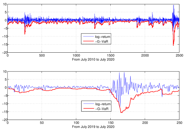
Figure 1: G-VaR value for log-return of S&P500 Index and the dynamic value of log-returns of S&P500 Index with risk level $\alpha=0.05$.

In the first picture of Figure 1, the blue line denotes the log-returns of S&P500 Index, and the red line denotes the VaR under $-\text{G-VaR}_{\alpha}(Z_{t+1})$ model, and the time $t+1$ is from July 2010 to July 2020. Moreover, as per the second picture of Figure 1, the measure $\text{G-VaR}_{\alpha}(Z_{t+1})$ can capture the local changes of the log-returns of S&P500 Index.

We consider small-windows $5\leq K,L\leq 15$, which are used to estimate the maximum volatility $\tilde{\overline{\sigma}}_{t+1}$ and the volatility uncertainty index $\tilde{\kappa}_{t+1}$. The excellent performance of the G-VaR model in Figure 1 indicates that the worst-case distribution can capture the local changing of a log-return of S&P500 Index. Therefore, we comment that the small windows $K$ and $L$ are important for estimating the local maximum volatility and volatility uncertainty index. Furthermore, the one-period forecast maximum volatility $\tilde{\overline{\sigma}}_{t+1}$ and volatility uncertainty index $\tilde{\kappa}_{t+1}$ can be used to capture the quantile of the distribution of the log-returns of S&P500 Index. The count numbers of the violations of the log-returns of S&P500 Index are given as follows:

$$\begin{array}[]{ll}&m_{00}(h)=\#\{-\text{G-VaR}_{\alpha}(Z_{t+1})<Z_{t+1},-\text{G-VaR}_{\alpha}(Z_{t+2})<Z_{t+2},\ t_{0}<t\leq h\};\\ &m_{01}(h)=\#\{-\text{G-VaR}_{\alpha}(Z_{t+1})<Z_{t+1},-\text{G-VaR}_{\alpha}(Z_{t+2})>Z_{t+2},\ t_{0}<t\leq h\};\\ &m_{10}(h)=\#\{-\text{G-VaR}_{\alpha}(Z_{t+1})>Z_{t+1},-\text{G-VaR}_{\alpha}(Z_{t+2})<Z_{t+2},\ t_{0}<t\leq h\};\\ &m_{11}(h)=\#\{-\text{G-VaR}_{\alpha}(Z_{t+1})>Z_{t+1},-\text{G-VaR}_{\alpha}(Z_{t+2})>Z_{t+2},\ t_{0}<t\leq h\},\end{array}$$

where $t_{0}$ is the initial date which is used to forecast $\text{G-VaR}_{\alpha}(Z_{t_{0}+1})$, and $\#\{\cdot\}$ denotes the count numbers which satisfies the violation conditions. Furthermore, we set

$$m_{1}(h)=m_{11}(h)+m_{10}(h),\ m_{0}(h)=m_{00}(h)+m_{01}(h),$$

and

$$\begin{array}[]{ll}&{\displaystyle\hat{\alpha}(h)=\frac{m_{1}(h)}{m_{0}(h)+m_{1}(h)},\quad 1-\hat{\alpha}(h)=\frac{m_{0}(h)}{m_{0}(h)+m_{1}(h)};}\\ &{\displaystyle\pi_{01}(h)=\frac{m_{01}(h)}{m_{00}(h)+m_{01}(h)},\quad\pi_{11}(h)=\frac{m_{11}(h)}{m_{10}(h)+m_{11}(h)};}\\ &{\displaystyle\pi(h)=\frac{m_{01}(h)+m_{11}(h)}{m_{00}(h)+m_{01}(h)+m_{10}(h)+m_{11}(h)}.}\end{array}$$

To assess the predictive performance of the $\text{G-VaR}(Z_{t+1})$ model, we use the test of a likelihood ratio for a Bernoulli trial and the test of a Christofferson independent to verify it. Let $\hat{\alpha}(h)$ be the sample violations rate and denote the likelihood ratio test statistics,

$$\mathbb{T}_{1}(h)=2m_{1}(h)\ln\frac{\hat{\alpha}(h)}{\alpha}+2m_{0}(h)\ln\frac{1-\hat{\alpha}(h)}{1-\alpha},$$

and the Christofferson independent test statistics,

$$\mathbb{T}_{2}(h)=2\ln\left[\frac{(1-\pi_{01}(h))^{m_{00}(h)}(\pi_{01}(h))^{m_{01}(h)}(1-\pi_{11}(h))^{m_{10}(h)}(\pi_{11}(h))^{m_{11}(h)}}{(1-\pi(h))^{m_{00}(h)+m_{10}(h)}(\pi(h))^{m_{01}(h)+m_{11}(h)}}\right].$$

Applying the well-known asymptotic $\chi^{2}(1)$ distribution, the $p$-value of the test is,

$$\text{LR}_{uc}^{h}=P\left(\chi^{2}(1)>\mathbb{T}_{1}(h)\right),$$

and independent test of violations point,

$$\text{LR}_{ind}^{h}=P\left(\chi^{2}(1)>\mathbb{T}_{2}(h)\right).$$

In the following, we conclude the testing results of S&P500 Index with $\alpha=0.05$.

Table 1: Testing results of S&P500 Index with $\alpha=0.05$

Model	Time	$h-t_{0}$	$\hat{\alpha}(h)$	$\text{LR}_{uc}^{h}$	$\text{LR}_{ind}^{h}$	$100\overline{\text{VaR}}$
G-VaR:	201907-202007	250	0.068	0.215	0.115	2.987
	201607-202007	1000	0.048	0.770	0.102	1.685
	201007-202007	2500	0.052	0.715	0.890	1.640

In Table 1, we consider three lengths of dates—one year, four years, and ten years. We calculate the indices $\hat{\alpha}(h)$, $\text{LR}_{uc}^{h}$, $\text{LR}_{ind}^{h}$, and $100\overline{\text{VaR}}$, respectively, where $100\overline{\text{VaR}}$ is 100 times VaR under G-VaR. It should be noted that

$$\text{LR}_{uc}^{h}>0.05,\quad\text{LR}_{ind}^{h}>0.05,$$

thus, the likelihood ratio test statistics and the Christofferson independent test statistics are through under the confidential level $95\%$.

4.1 Comparison with others VaR models

As [14] pointed out, the best VaR predictions for the benchmark are obtained by AR-GARCH filtered modeling such as the recommended AR-GARCH-Skewed-t or AR-GARCH-Skewed-t-EVT models. In [23], the G-VaR predictor is compared with these two models and a more traditional AR-GARCH-Normal predictor. Hence, we use the dataset S&P500 Index from January 3, 2000 to February 7, 2018 in [23], to compare the models developed in this study with the above four models. We denote ${\text{G-VaR}}^{*}$ as the VaR model developed in [23]. Partial results of Table 2 were downloaded from Table 7 of [23] with historical data window $W=250$. In Table 2, the G-VaR model with parameter $(K,L,N)=(5,10,100)$ under risk level $\alpha=0.05$ and $(K,L,N)=(6,5,100)$ under risk level $\alpha=0.01$.

Table 2: Testing results of S&P500 Index under VaR models

Model	Times	$\alpha$	$\hat{\alpha}(h)$	$\text{LR}_{uc}^{h}$	$\text{LR}_{ind}^{h}$	$100\overline{\text{VaR}}$
G-VaR:	200101-201802	0.05	0.051	0.84	0.99	1.87
	200101-201802	0.01	0.011	0.76	1.00	3.02
${\text{G-VaR}}^{*}$:	200101-201802	0.05	0.050	0.88	0.00	1.83
	200101-201802	0.01	0.010	0.87	0.00	3.46
GARCH(1,1)-N:	200101-201802	0.05	0.062	0.00	0.62	1.65
	200101-201802	0.01	0.026	0.00	0.19	2.35
GARCH(1,1)-St:	200101-201802	0.05	0.060	0.01	0.74	1.69
	200101-201802	0.01	0.014	0.01	0.23	2.68
GARCH(1,1)-St-EVT:	200101-201802	0.05	0.052	0.59	0.40	1.80
	200101-201802	0.01	0.014	0.01	0.06	2.71

In Table 2, we show the testing results of S&P500 Index under the VaR models: G-VaR, ${\text{G-VaR}}^{*}$, GARCH(1,1)-N, GARCH(1,1)-St, and GARCH(1,1)-St-EVT. We denote the values of the likelihood ratio test $\text{LR}_{uc}^{h}$ and the Christofferson independent test $\text{LR}_{ind}^{h}$ as boldface Type, which are through the tests under the confidential level $95\%$. We can see that the ${\text{G-VaR}}^{*}$ model in [23] is the best model among the above VaR models based on the value $\text{LR}_{uc}^{h}$. ${\text{G-VaR}}^{*}$ model can capture the long-time average loss of S&P500 Index. In fact, it should be noted that $\text{LR}_{uc}^{h}$ can test the accuracy of the VaR model and $\text{LR}_{ind}^{h}$ can test the independence of the violation points. Combining the values of $\text{LR}_{uc}^{h}$ and $\text{LR}_{ind}^{h}$, we can see that models G-VaR and GARCH(1,1)-St-EVT are the best for $\alpha=0.05$, and G-VaR is the best for $\alpha=0.01$. In particular, we also use the G-VaR model to predict VaR for NASDAQ Composite Index and CSI300, and we have a performance similar to that of G-VaR model, as shown in Table 2. Hence, we can see that the autoregressive models developed in this study are powerful tools to investigate the excellent performance of the G-VaR model.

5 Conclusion

Sublinear expectation is a powerful theoretical framework for measuring the probabilistic and distributional uncertainties inherent in many time sequences. Based on the central limit theorem in the theory of sublinear expectation, many important financial time series need to be assumed to follow the law of $G$-normal distribution in which the volatility uncertainty is naturally taken into account. It turns out that compared with many widely used VaR algorithms, the corresponding $G$-VaR is a much more robust and efficient financial risk measure (see Section 4).

Based on the assumption that the time series satisfies a G-normal distribution under sublinear expectation, we use a worst-case distribution to capture the robust distribution property of the time series, where the G-normal distribution denotes an infinite family of distributions. In [23], the empirical analysis is given based on an adaptive window $W_{0}$, which can capture the long-time loss of the time series, but is unable to follow the local changing of the time series. Diverging from [23], we develop a concept of Localization Windows to estimate the local sample variance. Then, combining the autoregressive models, we can obtain a one-period forecast maximum volatility, minimum volatility, and volatility uncertainty index. In Section 4, we apply this new mechanism to predict the VaR of S&P500 Index by the $\text{G-VaR}_{\alpha}(\cdot)$ model, which shows the advantage of using the autoregressive models and the Localization Windows.

References

- Artzner et al. [1999] P. Artzner, F. Delbaen, J.-M. Eber, and D. Heath. Coherent measures of risk. Mathematical Finance, 9:203–228, 1999.
- Avellaneda et al. [1995] M. Avellaneda, A. Levy, and A. Parás. Pricing and hedging derivative securities in markets with uncertain volatilities. Applied Mathematical Finance, 2:73–88, 1995.
- Chen and Epstein [2002] Z. Chen and L. Epstein. Ambiguity, risk, and asset returns in continuous time. Econometrica, 70(4):1403–1443, 2002.
- Cont [2006] R. Cont. Model uncertainty and its impact on the pricing of derivative instruments. Mathematical Finance, 16:519–547, 2006.
- Denis and Martini [2006] L. Denis and C. Martini. A theoretical framework for the pricing of contingent claims in the presence of model uncertainty. Annal of Applied Probability, 16:827–852, 2006.
- Epstein and Ji [2013] L. G. Epstein and S. Ji. Ambiguous volatility and asset pricing in continuous time. Review of Financial Studies, 26(7):1740–1786, 2013.
- Fang et al. [2019] X. Fang, S.G. Peng, Q.M. Shao, and Y.S. Song. Limit theorems with rate of convergence under sublinear expectations. Bernoulli, 25(4A):2564–2596, 2019.
- Föllmer and Schied [2011] H. Föllmer and A. Schied. Stochastic Finance. An Introduction in Discrete Time. Third revised and extended edition. Walter de Gruyter & Co., Berlin, 2011.
- Hu et al. [2017] M.S. Hu, S.G. Peng, and Y.S. Song. Stein type characterization for g-normal distributions. Electron. Commun. Probab., 22:1–12, 2017.
- Huber [1981] P. J. Huber. Robust Statistics. Wiley Series in Probability and Mathematical Statistics. John Wiley & Sons, Inc., New York, 3rd edition, 1981.
- Jin and Peng [2016] H. Jin and S. Peng. Optimal unbiased estimation for maximal distribution. arXiv:1611.07994v1, 2016.
- Kerkhof et al. [2010] J. Kerkhof, B. Melenberg, and H. Schumacher. Model risk and capital reserves. Journal of Banking & Finance, 34:267–279, 2010.
- Krylov [2020] N.V. Krylov. On shige peng’s central limit theorem. Stochastic Processes and their Applications, 130(3):1426–1434, 2020.
- Kuester et al. [2006] K. Kuester, S. Mittnik, and M. S. Paolella. Value-at-Risk Prediction: A comparison of alternative strategies. Journal of Financial Econometrics, 4(1):53–89, 2006.
- Lyons [1995] T. J. Lyons. Uncertain volatility and the risk-free synthesis of derivatives. Applied Mathematical Finance, 2:117–133, 1995.
- Peng [1997] S. Peng. Backward SDE and related g-expectation. Backward stochastic differential equations (Paris, 1995-1996) 141-159. Pitman Res. Notes Math. Ser., Longman, Harlow, 1997.
- Peng [2004] S. Peng. Filtration consistent nonlinear expectations and evaluations of contingent claims. Acta Mathematicae Applicatae Sinica, 20:1–24, 2004.
- Peng [2005] S. Peng. Nonlinear expectations and nonlinear Markov chains. Acta Mathematicae Applicatae Sinica, 26B:159–184, 2005.
- Peng [2006] S. Peng. Stochastic Analysis and Applications: The Abel Symposium 2005, chapter ”-expectation, -Brownian motion and related stochastic calculus of Itô type”. Springer, Berlin Heidelberg, 2006.
- Peng [2008] S. Peng. Multi-dimensional G-Brownian motion and related stochastic calculus under G-expectation. Stochastic Processes and Their Applications, 118:2223–2253, 2008.
- Peng [2017] S. Peng. Theory, methods and meaning of nonlinear expectation theory. Scientia Sinica Mathematica: In Chinese, 47:1223–1254, 2017.
- Peng [2019] S. Peng. Nonlinear Expectations and Stochastic Calculus under Uncertainty, pages 1–212. Springer, Berlin, Heidelberg, 2019.
- Peng et al. [2020] S. Peng, S. Yang, and J. Yao. Improving value-at-risk prediction under model uncertainty. arXiv:1805.03890:1–42, 2020.
- Song [2019] Y.S. Song. Stein’s method for law of large numbers under sublinear expectations. arXiv:1904.04674, pages 1–12, 2019.
- Song [2020] Y.S. Song. Normal approximation by stein’s method under sublinear expectations. Stochastic Processes and their Applications, 130(5):2838–2850, 2020.
- Walley [1991] P. Walley. Statistical Reasoning with Imprecise Probabilities. Chapman and Hall, 1991.