Towards a general quasi-linear approach for the instabilities of bi-Kappa plasmas. Whistler instability

Abstract

Kappa distributions are ubiquitous in space and astrophysical poorly collisional plasmas, such as the solar wind, suggesting that microscopic and macroscopic properties of these non-equilibrium plasmas are highly conditioned by the wave-particle interactions. The present work addresses the evolution of anisotropic bi-Kappa (or bi-$\kappa$-)distributions of electrons triggering instabilities of electromagnetic electron-cyclotron (or whistler) modes. The new quasi-linear approach proposed here includes time variations of the $\kappa$ parameter during the relaxation of temperature anisotropy. Numerical results show that $\kappa$ may increase for short interval of times at the beginning, but then decreases towards a value lower than the initial one, while the plasma beta and temperature anisotropy indicate a systematic relaxation. Our results suggest that the electromagnetic turbulence plays an important role on the suprathermalization of the plasma, ultimately lowering the parameter $\kappa$. Even though the variation of $\kappa$ is in general negative ($\Delta\kappa<0$) this variation seems to depend of the initial conditions of anisotropic electrons, which can vary very much in the inner heliosphere.

Keywords: Vlasov quasi-linear theory, Whistler electron-cyclotron instability, Kappa distributions

1 Introduction

There is currently an increasing interest for understanding the complex activity of the Sun, conditioning the space weather and with direct or indirect consequences on planetary environments and our terrestrial climate and technologies. The huge amount of kinetic energy released by the solar outflows, from slow to fast winds, or during coronal mass ejections (CMEs), accumulates in the solar wind mainly as kinetic anisotropies of plasma particles, namely, temperature anisotropies or self-focused beaming populations. At large heliospheric distances, e.g., 1 Astronomical Unit (AU), near the Earth’s orbit, the solar wind is a collisionless non-equilibrium plasma. It is well-known that in astrophysical and space environments when collisions are inefficient, plasma particle velocity distribution function (VDF) easily develop non-thermal characteristics that can provide the necessary free energy to excite self-generated instabilities, so called micro-instabilities. The excitation and relaxation of these instabilities play an important role, especially at kinetic scales in space plasma systems, such as the solar wind [1, 2, 3, 4] and the Earth’s magnetosphere [5, 6, 7].

For a realistic characterization of the enhanced wave fluctuations contributing to the relaxation process, the proposed kinetic approaches need also a realistic representation of the particle VDFs, according to the observations. Standard bi-Maxwellian model (i.e., Maxwellian distribution function with two temperatures) offers the simplest way to model magnetized plasma populations with anisotropic temperatures, $T_{\parallel}\neq T_{\perp}$, where $\parallel$ and $\perp$ define directions relative to the local magnetic field lines (gyrotropic distributions). Different combinations between temperature anisotropy and plasma beta ($\beta_{\parallel}=8\pi nk_{B}T_{\parallel}/B^{2}_{0}$) (where $n$, $k_{B}$ and $B_{0}$ represent the plasma density, the Boltzmann constant and the strength of the background magnetic field, respectively) will lead to different conditions for various kinetic instabilities. Anisotropic electrons with $T_{\perp}/T_{\parallel}>1$ trigger instabilities (predominantly right-handed polarized for small angles of propagation) [8, 9, 10, 11], while the left-handed parallel or oblique firehose instabilities are excited for $T_{\perp}/T_{\parallel}+2/\beta_{\parallel}<1$ [12, 13, 14].

Analogous to a bi-Maxwellian, the bi-Kappa model was introduced to describe anisotropic distributions with suprathermal tails [15]. Kappa models consistently reproduce the distributions of plasma particles in the magnetosphere and solar wind, i.e., electrons [see e.g. 16, 17, 18, 19, 7], and for ions [e.g. 20, 21, 22, 7]. High-energy (power-law) tails of Kappa distributions are enhanced by the suprathermal populations, and can markedly modify the dispersion and (in)stability conditions, at both electron and ion scales [23, 24, 25, 14, 26, 10, 27]. The analysis should take into account not only the parameters quantifying the kinetic anisotropy but also the abundance of suprathermals, in this case the $\kappa$ parameter.

Wave-particle interactions can alter the shape of the VDF and therefore the macroscopic properties of the plasma through a complex non-linear process. One traditional way to include non-linear effects of kinetic instabilities is the quasi-linear (QL) or weak turbulence theory [28, 29, 30]. QL approaches have been developed for temperature anisotropy driven instabilities in both, bi-Maxwellian and bi-Kappa distributed plasmas. In the solar wind conditions QL relaxation of bi-Maxwellian anisotropic plasmas (with $T_{\perp}/T_{\parallel}\neq 1$) show a good agreement, qualitatively and quantitatively, with fully non-linear particle simulations [see e.g. 31, 32, 33, 34, 35]. Extended to bi-Kappa distributed plasmas the same QL procedure shows that suprathermals can modify the time-scales of temperature anisotropy instabilities, accelerating the excitation and relaxation processes [see e.g. 36, 10, 37]. However, in this case comparisons between QL results and the higher order non-linear simulations, such as Vlasov-Maxwell solvers [36] or Particle-In-Cell (PIC) simulations [10] may not show the same good agreement as in the case of their bi-Maxwellian counterpart. [36, 10] suggest that such disagreement is mainly owed to the fact that QL approaches for Kappa distributions are constrained to keep $\kappa$ parameter fixed in time, whereas in PIC or Vlasov-Maxwell simulations the same parameter appears to evolve, an evolution that, by construction, cannot be achieved in a constrained QL model.

In this paper we address this issue by proposing a new QL approach for modeling the growth and saturation of instabilities and the relaxation of bi-Kappa distributions. Besides the time variation of the main moments quantifying the anisotropic temperature components, $T_{\parallel,\perp}$, our approach also accounts for a temporal variation of the $\kappa$ parameter. To do so, we consider the electromagnetic electron-cyclotron (EMEC) instability, also known as whistler instability, which is driven by anisotropic electrons with $T_{\perp}>T_{\parallel}$. The basic dispersion relations obtained from linear (Vlasov-Maxwell) theory are presented in section 2, while in Section 3 we derive the QL equations for the EMEC instability, by including $\kappa\to\kappa(t)$ as a function of time. In the present analysis we propose a zero-order approximation, which assumes the quasi-thermal core dominating the dynamics and evolving independently of suprathermals. In our model we consider that all the electrons follow a bi-Kappa velocity distribution. However, due to their high number density ($>$ 90% of total density), and by their kinetic energy density [38], the core electrons may dominate the dynamics. Therefore, here we build a zero order approximation, assuming an evolution of the core decoupled from that of suprathermals in the tails, and implicitly from the variation of kappa index. Numerical results are presented and discussed in detail in Section 4, analysing systematically different cases and taking several selections for the initial values of temperature anisotropy, plasma beta and $\kappa$. Finally, in Section 5 we summarize our findings and discuss the insights obtained, along with perspectives of better understanding of the dynamics of collisionless plasma in the solar wind.

2 Vlasov linear dispersion relation: Kappa vs. Maxwellian

For our model we consider a quasi-neutral magnetized plasma composed by electrons and ions, in which electrons follow a bi-Kappa velocity distribution function (VDF) given by

$$f(v_{\perp},v_{\parallel})=\frac{n_{0}}{\pi^{3/2}\theta_{\perp}^{2}\theta_{\parallel}}\frac{\Gamma(\kappa)}{\kappa^{1/2}\Gamma(\kappa-1/2)}\Biggl{(}1+\frac{v_{\perp}^{2}}{\kappa\theta_{\perp}^{2}}+\frac{v_{\parallel}^{2}}{\kappa\theta_{\parallel}^{2}}\Biggr{)}^{-\kappa-1},$$ (1)

where $n_{0}$ is the total number density, and $\kappa$ is the power-law exponent quantifying the abundance of suprathermal particles in the high-energy tails (suprathermalization) of our (bi-)Kappa distribution model. Velocity parameters $\theta_{\parallel,\perp}$ used for the normalization of perpendicular and parallel components of the velocity in Eq. (1) relate to the corresponding components $T_{\parallel,\perp}$ of the (kinetic) temperature $T=(T_{\parallel}+2\,T_{\perp})/3$, defined as the second order moment of the bi-Kappa distribution function.

$$T_{\parallel}=\frac{m_{e}\theta_{\parallel}^{2}}{2k_{B}}\frac{\kappa}{\kappa-3/2},\qquad T_{\perp}=\frac{m_{e}\theta_{\perp}^{2}}{2k_{B}}\frac{\kappa}{\kappa-3/2}\,,$$ (2)

where $k_{B}$ is the Boltzmann constant and $m_{e}$ the electron mass.

If $\kappa$ increases, lowering the high-energy tails, in the limit case of $\kappa\to\infty$ we approach the bi-Maxwellian (quasi-)thermal core of our bi-Kappa model [39, 14]

$$f_{M}(v_{\perp},v_{\parallel})=\frac{1}{\pi^{3/2}\theta_{\perp}^{2}\theta_{\parallel}}\exp\Biggl{(}-\frac{v_{\perp}^{2}}{\theta_{\perp}^{2}}-\frac{v_{\parallel}^{2}}{\theta_{\parallel}^{2}}\Biggr{)}$$ (3)

with components of the core temperature, $\Theta=(\Theta_{\parallel}+2\Theta_{\perp})/3$, defined by

$$\Theta_{\parallel}=\frac{m_{e}\theta_{\parallel}^{2}}{2k_{B}},\qquad\Theta_{\perp}=\frac{m_{e}\theta_{\perp}^{2}}{2k_{B}}.$$ (4)

Thus, with Eq. (2) in (4) we find the relationship between the Kappa temperatures ($T$, $T_{\perp,\parallel}$) and the core temperatures ($\Theta$, $\Theta_{\perp,\parallel}$)

$$T_{\perp}=\Theta_{\perp}\,\frac{\kappa}{\kappa-3/2},\qquad T_{\parallel}=\Theta_{\parallel}\,\frac{\kappa}{\kappa-3/2},\qquad T=\Theta\,\frac{\kappa}{\kappa-3/2},$$ (5)

Eqs. (5) suggest already that time variation of the Kappa temperatures may actually involve time variations of the core temperatures and the $\kappa$ parameter as well, as we will see below. It is also important to mention that in the limit $\kappa\to\infty$ we have $T\to\Theta$ (the most probable speed for Kappa becomes thermal speed for Maxwellian) [17, 39, 40].

In the case of bi-Kappa VDFs, the Vlasov linear dispersion relation for right-hand (RH) polarized waves propagating in the direction of the background magnetic field $\mathbf{B_{0}}$ is given by [see e.g 14, 36, and references therein]

$$\frac{c^{2}k_{\parallel}^{2}}{\omega_{pe}^{2}}=\left(\frac{T_{\perp}}{T_{\parallel}}-1\right)+\left[\frac{T_{\perp}}{T_{\parallel}}\,\omega-\left(\frac{T_{\perp}}{T_{\parallel}}-1\right)|\Omega_{e}|\right]\frac{1}{k_{\parallel}\theta_{\parallel}}\,Z_{\kappa}\left(\frac{\omega-|\Omega_{e}|}{k_{\parallel}\theta_{\parallel}}\right)\,,$$ (6)

where $\omega$ and $k_{\parallel}$ are the wave frequency and wavenumber, respectively, and $\omega_{pe}=\sqrt{4\pi n_{0}e^{2}/m_{e}}$ and $\Omega_{e}=eB_{0}/m_{e}c$ are the electron plasma frequency and gyrofrequency. Also, $e$ is the elementary charge, $c$ is the speed of light, and

$$Z_{\kappa}(\xi)=\frac{1}{\pi^{1/2}\kappa^{1/2}}\frac{\Gamma(\kappa)}{\Gamma(\kappa-1/2)}\int_{-\infty}^{\infty}dx\,\frac{(1+x^{2}/\kappa)^{-\kappa}}{x-\xi},\qquad{\rm Im}(\xi)>0$$ (7)

is the Modified Dispersion function [15, 41, 26]. It is important to mention that in the Maxwellian limit $\kappa\to\infty$ $Z_{k}$ becomes the well-known Plasma Dispersion Function $Z$ defined by Fried and Conte [42].

$$Z(\xi)=\frac{1}{\pi^{1/2}}\int_{-\infty}^{\infty}dx\,\frac{\exp(-x^{2})}{x-\xi},\qquad{\rm Im}(\xi)>0.$$ (8)

In the same limit $\kappa\to\infty$ Eq. (6) becomes specific for the bi-Maxwellian core, and will be use in the next to describe the core contribution independent of suprathermals in the high energy tails.

Table 1: Electron plasma parameters used in the present study^∗.

Case	$A$	$\beta_{c,\parallel}$	$\kappa$	$\beta_{\parallel}$
	4.0	0.05	3.0	0.10
Case I	4.0	0.50	3.0	1.00
	4.0	5.00	3.0	10.0
	4.0	0.50	1.6	8.00
Case II	4.0	0.50	3.0	1.00
	4.0	0.50	8.0	0.62
	2.0	0.50	3.0	1.00
Case III	4.0	0.50	3.0	1.00
	8.0	0.50	3.0	1.00

^∗In all cases we consider $\omega_{pe}/\Omega_{e}=20$, and cold ions.

For temperature anisotropy

$$A=\frac{T_{\perp}}{T_{\parallel}}=\frac{\Theta_{\perp}}{\Theta_{\parallel}}>1,$$ (9)

the dispersion relation Eq. (6) is unstable to whistler electron-cyclotron electromagnetic (EMEC) waves, with a maximum growth rate that increases with increasing temperature anisotropy $A>1$ and increasing parallel plasma beta $\beta_{\parallel}=8\pi n_{0}k_{B}T_{\parallel}/B^{2}_{0}$ [see e.g. 8, and references therein]. As mentioned in Section 1, this behaviour is similar for any collisionless plasma composed by anisotropic electrons, and in the case of $\kappa$-distributed electrons, several studies have been presented in the last few years [25, 14, 36, 10]. Here we consider three cases with different combinations of temperature anisotropy, plasma beta and the $\kappa$ parameter as shown in Table 1. To make a proper comparison between Kappa and its Maxwellian core (subscript $c$), as a limit case $\kappa\to\infty$, we need to differentiate between their beta parameters

$$\beta_{\parallel}=\frac{8\pi n_{0}k_{B}T_{\parallel}}{B^{2}_{0}}=\frac{8\pi n_{0}k_{B}\Theta_{\parallel}}{B^{2}_{0}}\,\left(\frac{\kappa}{\kappa-3/2}\right)=\beta_{c,\parallel}\,\left(\frac{\kappa}{\kappa-3/2}\right)\,,$$ (10)

with $\beta_{\parallel}\to\beta_{c,\parallel}$ when $\kappa\to\infty$. Thus, to make a proper comparison between our cases, here we need to consider variations of the independent one, i.e., $\beta_{c,\parallel}$, associated with the core.

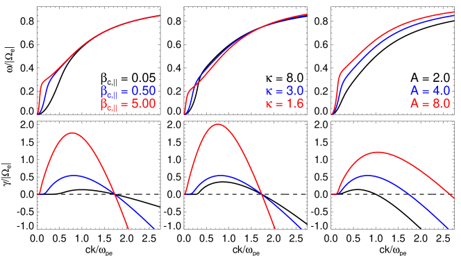
Figure 1: Dispersion relation for Case I (left), Case II (center), and Case III (right) with plasma parameters as shown in Table 1. Top and bottom panels show the real and imaginary parts of the frequency as a function of wavenumber, expressed in units of the electron gyrofrequency and inertial length, respectively.

Fig. 1 shows the wave-number linear dispersion of the wave (real) frequency, $\omega$, and the growth rate (imaginary), $\gamma$, for fixed $\kappa$ and anisotropy, and varying $\beta_{c,\parallel}$ (Case I, left); fixed anisotropy and $\beta_{c,\parallel}$, and varying $\kappa$ (Case II, center); and fixed $\kappa$ and $\beta_{c,\parallel}$ with different anisotropy values (Case III, right), considering plasma parameters detailed in Table 1. With this systematic variation of the three main parameters controlling the dispersion relation is clear that when all other parameters are fixed, $\gamma$ increases with increasing $\beta_{c,\parallel}$, $A$, and decreasing $\kappa$ (see bottom panels in the figure). Thus, as during QL relaxation the energy of the electromagnetic waves grows at the expense of temperature anisotropy (which means also variations of the plasma beta), if the value of $\kappa$ also determines the level of the instability, it is expected $\kappa$ to also evolve as the instability develops. In other words, if the anisotropy and beta parameters are not constant during the evolution of the plasma, then $\kappa$ should not remain constant either. However, as QL evolution of the EMEC instability produces a negative variation of the anisotropy ($dA/dt<0$) and a positive variation of parallel beta ($d\beta_{\parallel}/dt<0$), the sign of $d\kappa/dt$ remains still unclear. We will address this topic in the next section.

3 Quasi-linear evolution with a dynamic $\kappa$

To find a consistent model to account for a QL relaxation with $d\kappa/dt\neq 0$ we start from the traditional QL approach. Following Lazar et al. (2017) [36], using QL theory we find the equations describing the EMEC instability that are given by the time derivatives of both temperatures

$$\frac{dT_{\perp}}{dt} = -\frac{e^{2}}{m_{e}k_{B}}\int_{-\infty}^{\infty}\frac{dk_{\parallel}}{c^{2}k_{\parallel}^{2}}\,\omega_{i}(k_{\parallel})\left(\frac{c^{2}k_{\parallel}^{2}}{\omega_{pe}^{2}}+\frac{1}{2}\right)\delta B^{2}(k_{\parallel}),$$ (11)

$$\frac{dT_{\parallel}}{dt} = \frac{e^{2}}{m_{e}k_{B}}\int_{-\infty}^{\infty}\frac{dk_{\parallel}}{c^{2}k_{\parallel}^{2}}\,\omega_{i}(k_{\parallel})\left(\frac{c^{2}k_{\parallel}^{2}}{\omega_{pe}^{2}}+1\right)\delta B^{2}(k_{\parallel}),$$ (12)

and the wave energy density equation

$$\frac{\partial\delta B^{2}(k_{\parallel})}{\partial t}=2\omega_{i}(k_{\parallel})\,\delta B^{2}(k_{\parallel}).$$ (13)

In the case of bi-Maxwellian distributions, Eqs. (11)-(13) together with the dispersion relation Eq. (6) provide a closed system of differential equations. However, in the case of bi-Kappa distribution, from the expressions of temperatures in Eqs. (5), their variation in time, i.e., $dT_{\parallel,\perp}/dt$ implies variations in time not only for $\Theta_{\parallel,\perp}$ (as assumed in a simplified model with fixed $\kappa$) but also for the exponent $\kappa$

$$\frac{3}{2\kappa(\kappa-3/2)}\frac{d\kappa}{dt}=\frac{1}{\Theta}\frac{d\Theta}{dt}-\frac{1}{T}\frac{dT}{dt}\,.$$ (14)

$\kappa$ couples both time variations of the temperature components, such that, at least at $t=0$, the anisotropy of bi-Kappa distribution is the same with the anisotropy of bi-Maxwellian core, as shown in Eq. (9). These variations can be studied for two distinct cases. First, if $\kappa=\kappa_{0}=$ constant, the relaxation of the temperature anisotropy is achieved by $dT_{\perp}\leq 0$ and $dT_{\parallel}\geq 0$, such that $dA/dt<0$, which implies that $d\Theta_{\perp}\leq 0$ and $d\Theta_{\parallel}\geq 0$ [see e.g 36, 10, 37]. On the other hand, if $\kappa$ changes in time, i.e., $\kappa=\kappa(t)$ (an evolution suggested by the Vlasov simulations in Ref. [36]), the QL evolution of the growing fluctuations involves the relaxation of bi-Kappa VDF and is described by the time variation of seven variables, i.e., $T_{\perp,\parallel}$, $\delta B$, $\omega_{i}$, $\kappa$, and also $\Theta_{\perp,\parallel}$. However, we only have five equations of evolution, i.e., Eqs. (11)-(14), and the dispersion relation Eq. (6), and need two more independent equations, e.g., for the evolution of the core temperatures $\Theta_{\perp,\parallel}$. Here we propose a zero-order approximation which assumes the dynamics dominated by the quasi-thermal core, with an evolution described (independently of suprathermals) by the following QL equations

$$\frac{d\Theta_{\perp}}{dt} = -\frac{e^{2}}{m_{e}k_{B}}\int_{-\infty}^{\infty}\frac{dk_{\parallel}}{c^{2}k_{\parallel}^{2}}\,\omega_{i}^{c}(k_{\parallel})\left(\frac{c^{2}k_{\parallel}^{2}}{\omega_{pe}^{2}}+\frac{1}{2}\right)\delta B_{c}^{2}(k_{\parallel}),$$ (15)

$$\frac{d\Theta_{\parallel}}{dt} = \frac{e^{2}}{m_{e}k_{B}}\int_{-\infty}^{\infty}\frac{dk_{\parallel}}{c^{2}k_{\parallel}^{2}}\,\omega_{i}^{c}(k_{\parallel})\left(\frac{c^{2}k_{\parallel}^{2}}{\omega_{pe}^{2}}+1\right)\delta B_{c}^{2}(k_{\parallel}).$$ (16)

Note that Eqs. (15)-(16) are the correspondent equations to Eqs. (11)-(12), but instead of the evolution of the bi-Kappa describe the evolution of bi-Maxwellian core ($f_{M}$) under the effects of whistler growing electromagnetic fields (EMEC instability)

$$\frac{\partial\delta B_{c}^{2}(k_{\parallel})}{\partial t}=2\omega_{i}^{c}(k_{\parallel})\,\delta B_{c}^{2}(k_{\parallel}),$$ (17)

triggered only by the anisotropic core with growth rate $\omega_{i}^{c}$ given by the dispersion relation

$$\frac{c^{2}k_{\parallel}^{2}}{\omega_{pe}^{2}}=\left(\frac{\Theta_{\perp}}{\Theta_{\parallel}}-1\right)+\left[\frac{\Theta_{\perp}}{\Theta_{\parallel}}\,\omega-\left(\frac{\Theta_{\perp}}{\Theta_{\parallel}}-1\right)|\Omega_{e}|\right]\frac{1}{k_{\parallel}\sqrt{2\Theta_{\parallel}/m}}\,Z\left(\frac{\omega-|\Omega_{e}|}{k_{\parallel}\sqrt{2\Theta_{\parallel}/m}}\right),$$ (18)

where $Z(x)$ is the standard plasma dispersion function characteristic to bi-Maxwellian plasmas, given by Eq. (8). As already mentioned, due to its high density ($>$ 90% of total density) we assume that the core dominates the dynamics, such that in this zero order approximation we can decouple the evolution of the core from the evolution of suprathermal tails, and implicitly from the variation of kappa index. In summary, Eqs. (15)-(16), completed by Eqs. (17)-(18), describe the time variation of the core, i.e., moments $\Theta_{\perp,\parallel}$, which can be then coupled to Eqs. (11)-(14) and (6) to model time variation of $\kappa$ parameter under QL theory.

4 Results

To solve the system of QL equations, we use a discrete grid in the wavenumber space (normalized to the electron inertial length) with 2000 points between $0.001<|ck_{\parallel}/\omega_{pe}<3$. All cases were ran up to $\Omega_{e}t=300$ with a time step of $dt=0.02/\Omega_{e}$, and the magnetic field spectrum was chose to be $\delta B^{2}(k_{\parallel})=10^{-5}B^{2}_{0}$ at $t=0$. Under this procedure, knowing the magnetic field spectrum and the value of the parameters at any given time $t$, we can solve the dispersion relation to find the complex frequency $\omega+i\gamma$, as a function of $k_{\parallel}$ at this particular time, to then evaluate the time derivative of each parameter. We then evolve the whole system to the next time step $t+dt$ with a 2nd order Runge-Kutta method. Using this scheme we solved the QL system for all 9 cases shown in Table 1 as initial conditions.

4.1 Case I. Varying plasma beta

First we consider the QL evolution of three initial conditions shown in Table 1 Case I, fixing temperature anisotropy and $\kappa$ parameter, and varying plasma beta. In Figure 2 left, center and right columns correspond to $\beta_{c,\parallel}(t=0)=0.05$, $0.5$ and $5.0$, respectively, $\kappa(t=0)=3$, and $A(t=0)=4$. In addition, with this selection of parameters we also have $\beta_{\parallel}(t=0)=0.1$ (left), $\beta_{\parallel}(t=0)=1.0$ (center), and $\beta_{\parallel}(t=0)=10.0$ (right). From top to bottom each row shows the time evolution of temperature anisotropy, the magnetic field energy, parallel and perpendicular temperature of the bi-Kappa, parallel and perpendicular temperature of the bi-Maxwellian core, and $\kappa$ parameter. Black and red curves represent the quantities associated with the bi-Maxwellian and bi-Kappa VDFs and the associated magnetic field energy. From the figure we can see that, as expected for the bi-Maxwellian core and the bi-Kappa, the decrease of temperature anisotropy (first row) drives the growth of the fluctuating fields (second row) while temperatures approach each other (third and fourth rows).

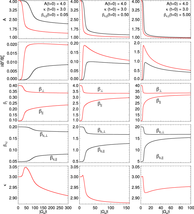
Figure 2: QL time evolution of the EMEC instability considering initial parameters from Table 1 Case I, fixing $\kappa(t=0)=3.0$, and $A(t=0)=4.0$ and varying $\beta_{c,\parallel}=0.05$ (left), $\beta_{c,\parallel}=0.5$ (center), and $\beta_{c,\parallel}=5.0$ (right). In all panels, red and black curves represent the evolution of the magnetic field and plasma parameters of the bi-Kappa or bi-Maxwellian core VDFs, respectively. From top to bottom each row shows temperature anisotropy, magnetic energy density, parallel and perpendicular plasma of the bi-Kappa, betas of the bi-Maxwellian core, and $\kappa$ parameter. In all panels, time is expressed in units of the electron gyrofrequency.

The main differences between each case (column) lie in the timescale of the process and the behavior of the $\kappa$ parameter (bottom row in Figure 2). From left to right each column shows a run with a larger initial growth rate, and therefore a shorter characteristic time for the QL relaxation (note that owing to this the extent of the time axis is different at each column). Even though in all three cases $\kappa$ increases at the beginning of the relaxation process, the time profile of $\kappa$ appears to be dependent on the initial value of beta. For $\beta_{\parallel}=10.0$ (right column), initially $\kappa$ exhibits a minimal increase. Then, following the fast relaxation of the temperature anisotropy, $\kappa$ rapidly decreases reaching a minimum value at the same time in which perpendicular temperatures finish their rapid decrease ($\Omega_{e}t\sim 9$), and finally slowly recovers to a level slightly higher. For $\beta_{\parallel}=1.0$, however, the center column of Figure 2 shows a different behavior. In this case the initial increase of $\kappa$, while still small, is about ten times larger compared to the previous case, and the later decrease of the $\kappa$ parameter remains monotonous until the end of the calculations. For $\beta_{\parallel}=0.1$ (left column in the figure) the initial increase of $\kappa$ is about ten time larger compared with the $\beta_{\parallel}=1.0$ case. In addition, here the changes occur at a considerably slower rate, but the final value of $\kappa$ is similar.

4.2 Case II. Varying the $\kappa$ parameter.

After analyzing the 3 cases shown in Figure 2 we can see that the time evolution of the $\kappa$ parameter is not trivial. $\kappa(t)$ is not even a monotonously increasing or decreasing function of time as the anisotropy or the temperatures. Here we continue the analysis by considering Case II initial values from Table 1, fixing parallel beta of the Maxwellian core and temperature anisotropy at $t=0$ to $\beta_{c,\parallel}=0.5$, and $A=4$, respectively, and selecting three different initial values for $\kappa$. Namely, $\kappa=1.6$ (left), $\kappa=3.0$ (center) and $\kappa=8.0$ (right), which implies $\beta_{\parallel}=8.0$, $1.0$, and $0.62$, respectively.

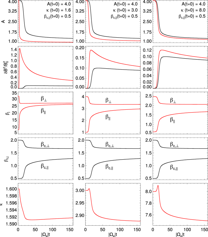
Figure 3: QL time evolution of the EMEC instability considering initial parameters from Table 1 Case II, fixing $A(t=0)=4.0$, and $\beta_{c,\parallel}(t=0)=0.5$ and varying $\kappa(t=0)=1.6$ (left), $\kappa(t=0)=3.0$ (center), and $\kappa(t=0)=8.0$ (right), which implies $\beta_{\parallel}=8.0$, $1.0$, and $0.62$, respectively. In all panels, red and black curves represent the evolution of the magnetic field and plasma parameters of the bi-Kappa or bi-Maxwellian core VDFs, respectively. From top to bottom each row shows temperature anisotropy, magnetic energy density, parallel and perpendicular plasma of the bi-Kappa, betas of the bi-Maxwellian core, and $\kappa$ parameter. In all panels, time is expressed in units of the electron gyrofrequency.

The QL evolution for this three cases are shown in Figure 3 where each panel represent the same as in Figure 2. These three cases with different initial $\kappa$ parameter (three columns in Figure 3) exhibit qualitatively the same time evolution, but all occurring faster and with a larger level of electromagnetic fluctuations for smaller initial $\kappa$ (larger initial $\beta_{\parallel}$. This is consistent with the situation shown in Figure 1, as a smaller value of $\kappa$ implies a larger growth rate and therefore a faster relaxation. In addition, from Figure 3 we also see that the absolute variation of $\kappa$ seem to scale with the value of $\kappa$, in line with Eq. (14). As $d\kappa/dt$ is proportional to $\kappa-3/2$, independent of the value of other plasma parameters, a larger initial value of $\kappa$ will always yield to a larger time variation of the same parameter. Finally, Figure 3 also shows that, even though the final value of $\kappa$ is smaller than $\kappa(t=0)$, the $\kappa$ parameter increases at the beginning of the relaxation, and the initial enhancement of $\kappa$ increases with increasing initial $\kappa$ value.

4.3 Case III. Varying temperature anisotropy.

To further characterize the evolution of $\kappa$ depending on the initial parameters we now fix $\beta_{c,\parallel}=0.5$ and $\kappa=3.0$ at $t=0$ (implying $\beta_{\parallel}(t=0)=1.0$, and consider three possibilities for the initial temperature anisotropy. Figure 4 shows the QL evolution for $A=2.0$ (left), $A=4.0$ (center), and $A=8.0$ (right) at $t=0$, with all other initial plasma parameters given by Case III in Table 1. From the figure we can see that this case is similar to the previous ones, but as expected from linear calculations here the initial anisotropy determines the time scale of the dynamics. The figure also shows that the initial temperature anisotropy also controls the shape of $\kappa$ as a function of time. In the same fashion as the cases shown in Figure 2 and Figure 3, for $A(t=0)=8.0$ and $A(t=0)=4.0$ the $\kappa$ parameter initially increases and then decreases, and the level of the initial increase depend on how fast the relaxation occurs. However, for $A(t=0)=2.0$ the $\kappa$ parameter only decreases with time. Thus, unlike Figure 2 in which a faster relaxation resulted in a smaller increase of $\kappa$, when the speed of the relaxation is determined by the initial temperature anisotropy, $\kappa$ reaches larger values for larger growth rate of the waves.

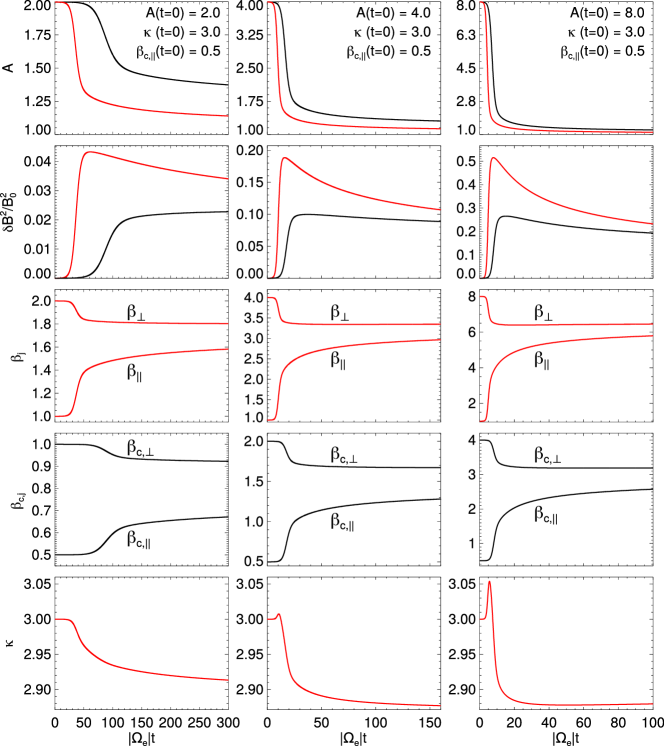
Figure 4: QL time evolution of the EMEC instability considering initial parameters from Table 1 Case III, fixing $\kappa(t=0)=3.0$, and $\beta_{c,\parallel}(t=0)=0.5$ ($\beta_{\parallel}(t=0)=1.0$), and varying $A(t=0)=2.0$ (left), $A(t=0)=4.0$ (center), and $A(t=0)=8.0$ (right). In all panels, red and black curves represent the evolution of the magnetic field and plasma parameters of the bi-Kappa or bi-Maxwellian core VDFs, respectively. From top to bottom each row shows temperature anisotropy, magnetic energy density, parallel and perpendicular plasma of the bi-Kappa, betas of the bi-Maxwellian core, and $\kappa$ parameter. In all panels, time is expressed in units of the electron gyrofrequency.

After considering all these cases a robust emerging result is that, regardless the initial value of the anisotropy, $\Delta\kappa=\kappa(t_{\rm{end}})-\kappa(t=0)\leq 0$, where $\kappa(t_{\rm{end}})$ is the value of $\kappa$ after the relaxation of the EMEC instability; i.e., independent of the details of each case, the QL relaxation of the EMEC instability produces an absolute decrease of $\kappa$. It is important to mention that this is consistent with Vlasov-Maxwell simulations presented in Ref. [36], in which, for almost all considered cases the triggering and relaxation of the EMEC instability led to a reduction of the $\kappa$ parameter in a qualitatively similar timescale.

4.4 Plasma beta and temperature anisotropy paths

We have already solved the equations of our QL model considering distinct combinations of the relevant initial plasma parameters (temperature anisotropy, plasma beta and $\kappa$). With such systematic study we were able to identify and characterize the effect of each parameter on the QL evolution of the EMEC instability. Here we complete our analysis by performing an ensemble of QL runs for different values of the initial $\kappa$ parameter ($1.6\leq\kappa(t=0)\leq 10.0$ and a parallel beta ($<0.1\leq\beta_{\parallel}(t=0)\leq 10.0$), and also fixing $A(t=0)=4.0$. With this procedure we can build paths in the $\beta_{\parallel}$, $A$ parameters space, and follow the dynamics of the EMEC instability triggered from different starting points at $t=0$ up to $|\Omega_{e}|t=300$, which is a long enough time scale for the development of the EMEC instability for all considered initial conditions.

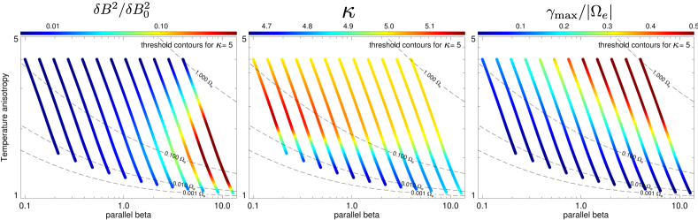
Figure 5: Time evolution in the ($\beta_{\parallel}$, $A$)-space, from an ensemble of QL calculations, starting from the same initial $A(t=0)=4$ and $\kappa_{0}=5$, up to $|\Omega_{e}|t=300$), for the fluctuating magnetic energy (left), $\kappa$ (middle) and $\gamma_{\rm max}$ (right). Dashed lines mark different maximum growth rate contours.

Figure 5 shows dynamical paths of the magnetic field energy (left panel), the $\kappa$ parameter (center), and the maximum growth rate of EMEC waves (right), during the relaxation of the EMEC instability for $\kappa(t=0)=5.0$ (other values of initial $\kappa$ exhibit similar results and therefore are not shown here). Regarding the magnetic field energy (left panel in the figure), as expected, the level of the electromagnetic fluctuations increases with increasing initial parallel beta. At the same time, the plasma evolves towards a less unstable state by reducing temperature anisotropy and increasing parallel plasma beta, with all dynamical paths collapsing to a EMEC instability level with $10^{-3}\Omega_{e}<\gamma<10^{-2}\Omega_{e}$ (dashed lines in the figure). In addition, looking a the evolution of $\kappa$ (central panel in Figure 5), we can see that in all cases the final value of $\kappa$ is less than the initial one ($\Delta\kappa<0$). At the same time, in all cases the maximum growth rate monotonically decreases in time (see right panel in Figure 5). Even though, as for fixed plasma beta and anisotropy the growth rate of the waves increases with decreasing $\kappa$, when the $\kappa$ parameter is allowed to change in time, the relaxation or saturation of the EMEC instability is achieved not only by the relaxation of the temperature anisotropy (as in the case of a bi-Maxwellian) but also by the decrease of the $\kappa$ parameter. Therefore, on the contrary to the case of bi-Maxwellian distributions, these results seem to indicate that for bi-Kappa distributions, the collisionless relaxation of the EMEC instability does not result in the thermalization of the plasma as such behavior would imply $\Delta\kappa>0$. Instead of thermodynamic equilibrium, the plasma does evolve towards stability, but in this case stability according to the Vlasov equation.

Finally, although for all cases $\Delta\kappa<0$, as already mentioned, the evolution and relaxation of the $\kappa$ parameter is considerably more complex than the relaxation of the temperature anisotropy. A closer look at the central panel of Figure 5 suggests that for $\kappa(t=0)=5.0$ there is a range of initial plasma beta values around $\beta_{\parallel}(t=0)\sim 0.5$, in which the reduction of $\kappa$ is maximum. If beta is too small $\kappa$ also decreases, but only after an initial increasing which is bigger for decreasing bet such that the addition of this two-steps process determines $\Delta\kappa$ to be small. On the other hand, if $\beta_{\parallel}(t=0)>1.0$, then the variation of $\kappa$ is also smaller. The same situation repeats for all considered initial $\kappa$ values as shown in Figure 6. From the figure we can see that for all considered initial $\kappa$ values, $\Delta\kappa$ is a negative function of beta with a clear minimum. For small initial $\kappa$ ($\kappa(t=0)=1.6$ or 2.0), the reduction of $\kappa$ is almost negligible and the maximum reduction of $\kappa$ is achieved with $\beta_{\rm{min}}\sim 0.5$. However, for all $\kappa\geq 3.0$ the initial beta allowing the largest variation of the $\kappa$ parameter is $\beta_{\rm{min}}\sim 0.37$, and that the maximum absolute variation of $\kappa$ increases with increasing $\kappa$. All these results confirm that the QL relaxation of the EMEC instability lead the plasma towards a Vlasov equilibrium (meaning the quasi-stationary state reached in the absence of collisions) and not necessarily thermodynamic equilibrium.

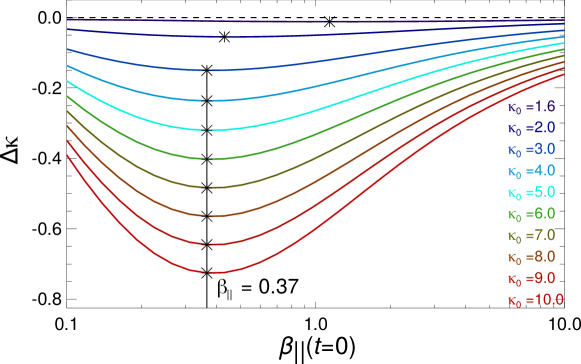
Figure 6: Difference between the value $\kappa$ after and before the QL relaxation as a function of initial parallel plasma beta. Each color correspond to a different initial $\kappa$ value, and black asterisk symbols mark the maximum $\kappa$ variation for each initial $\kappa$. For all $\kappa\geq 3.0$ the initial beta allowing the largest variation of the $\kappa$ parameter is $\beta_{\rm{min}}\sim 0.37$.

5 Conclusions

In this work we have introduced a new QL kinetic approach to account for the variations of all parameters characterizing a bi-Kappa distribution function during the excitation of whistler instability. Going one step further than previous moment-based QL works we have been able to address the variability and evolution of the $\kappa$ parameter due to wave-particle interactions, and find that indeed $\kappa$ is a dynamic parameter that can evolve during the excitation of this instability. A potential variation of $\kappa$ was already suggested by the fully non-linear simulations [43, 44, 36, 10], considering the time evolution of the whistler fluctuations and their feedback on the bi-Kappa distributed electrons.

Considering plasma parameters relevant to space environments such as the solar wind or planetary magnetospheres, we have performed a systematic study to analyze the dependence of the initial value of temperature anisotropy, plasma beta, and the $\kappa$ parameter. Our numerical results show that the time variation of $\kappa$ increases for higher initial values $\kappa(t=0)$, and that the time evolution of $\kappa(t)$ is not monotonic as in the case of temperature anisotropy that is constantly decreasing in time (or an increasing parallel plasma beta). In general, we found $\kappa$ increasing at the beginning of the QL evolution, and then decreasing towards a value smaller than the initial one, such that, overall $\Delta\kappa=\kappa(t_{\rm{end}})-\kappa(t=0)\leq 0$. As already mentioned, the plasma beta and anisotropy show different evolutions. The initial growth of $\kappa$ increases for larger initial temperature anisotropy, but decreases for decreasing initial parallel beta. In addition, the final variation of $\kappa$ ($|\Delta\kappa|$) exhibits a maximum value for initial parallel beta around $\beta_{\parallel}\sim 0.37$ for all $\kappa(t=0)\geq 3.0$, suggesting that for extreme values of beta the $\kappa$ power-index may not be affected by wave-particle interactions.

All these results show a variable $\kappa$ during the excitation of kinetic instabilities. The QL evolution of the EMEC instability results in a reduction of $\kappa$, such that plasma evolves towards Vlasov equilibrium, but not necessarily a thermodynamic (Maxwellian) equilibrium, which is somehow expected in the presence of a fluctuating EM power, low but still present in the system (preventing also the complete relaxation of temperature anisotropy). As shown in Figs. 2-5, the QL (partial) relaxation of the anisotropic temperature leads to an increased level of wave fluctuations in the plasma, such that the system achieves a new quasi-stationary (quasi-stable) state with an enhanced level of wave fluctuations which entertain and boost, evenly, the supathermals, ultimately lowering the parameter $\kappa$. Throughout all these processes the electromagnetic turbulence plays an important role on the suprathermalization of the plasma and may even determine the lower values of the kappa power-index [see e.g. 45].

Even though with this zero-order model the variations of $\kappa$ can be considered rather small, the consistency of the results here presented, and their good qualitative agreement with previous reports based on fully non-linear models [43, 36] suggests that QL approaches can be used as a powerful tool to study the non-linear evolution of poorly collisional plasmas. This is true for bi-Maxwellian plasmas in which density, temperatures and bulk velocity describe the dynamics of the system [see e.g. 34, and references therein], and the same should occur in the case of non-Maxwellian plasmas exhibiting non-thermal features such as power-law tails. We plan to address these aspects and other issues, expanding the scope of our model in subsequent works.

In summary, the fact that Kappa distributions are ubiquitous in many space and astrophysical plasmas, suggests that the enhanced fluctuations triggered by kinetic instabilities may play a key role on the regulation of these distributions in the inner heliosphere. Under this context, our new QL approach may improve the understanding of the processes that control and shape the velocity distribution function of plasma particles in poorly collisional plasmas. We expect these results to motivate the community to consider more realistic theoretical models, which complement the more idealized (bi-)Maxwellian description with $\kappa$ power exponents, or any other plasma parameter that can reproduce the observations. Such models are expected to be validated by the high resolution observations by the Solar Parker Probe or Solar Orbiter missions, which can couple particle and wave fluctuations from concomitant in-situ measurements.

References

- [1] Kasper J C, Lazarus A J and Gary S P 2002 Geophys. Res. Lett. 29 1839
- [2] Marsch E 2006 Living Rev. Solar Phys. 3
- [3] Bale S D, Kasper J C, Howes G G, Quataert E, Salem C and Sundkvist D 2009 Phys. Rev. Lett. 103 211101
- [4] Bruno R and Carbone V 2013 Living Rev. Solar Phys. 10 2
- [5] Heinemann M 1999 J. Geophys. Res. 104 28397–28410
- [6] Matsumoto Y and Hoshino M 2006 J. Geophys. Res. 111
- [7] Espinoza C M, Stepanova M, Moya P S, Antonova E E and Valdivia J A 2018 Geophys. Res. Lett. 45 6362–6370
- [8] Gary S P 1993 Theory of Space Plasma Microinstabilities (Cambridge University Press)
- [9] Gary S P and Karimabadi H 2006 J. Geophys. Res. 111 A11224
- [10] Lazar M, Yoon P H, López R A and Moya P S 2018 J. Geophys. Res. 123 6–19
- [11] López R A, Lazar M, Shaaban S M, Poedts S and Moya P S 2020 Astrophys. J. Lett. 900 L25
- [12] Camporeale E and Burgess D 2008 J. Geophys. Res. 113 A07107
- [13] Lazar M and Poedts S 2009 Solar Physics 258 119–128 ISSN 1573-093X
- [14] Viñas A F, Moya P S, Navarro R E, Valdivia J A, Araneda J A and Muñoz V 2015 J. Geophys. Res. 120
- [15] Summers D and Thorne R M 1991 Phys. Fluids B 3 1835–1847
- [16] Olbert S 1968 Summary of Experimental Results from M.I.T. Detector on IMP-1 (Astrophysics and Space Science Library vol 10) (Springer Netherlands) pp 641–659
- [17] Vasyliunas V M 1968 J. Geophys. Res. 73 2839–2884
- [18] Pilipp W G, Miggenrieder H, Montgomery M D, Mühlhäuser K H, Rosenbauer H and Schwenn R 1987 J. Geophys. Res. 92 1093–1101
- [19] Nieves-Chinchilla T and Viñas A F 2008 J. Geophys. Res. 113 A02105
- [20] Lockwood M, Bromage B J I, Horne R B, St-Maurice J P, Willis D M and Cowley S W H 1987 Geophys. Res. Lett. 14 111–114
- [21] Chotoo K, Collier M R, Galvin A B, Hamilton D C and Gloeckler G 1998 J. Geophys. Res. 103 17441–17445
- [22] Chotoo K, Schwadron N A, Mason G M, Zurbuchen T H, Gloeckler G, Posner A, Fisk L A, Galvin A B, Hamilton D C and Collier M R 2000 J. Geophys. Res. 105 23107–23122
- [23] Lazar M, Poedts S and Schlickeiser R 2011 Mon. Not. R. Astron. Soc. 410 663–670
- [24] dos Santos M S, Ziebell L F and Gaelzer R 2014 Phys. Plasmas 21 112102
- [25] Navarro R E, Muñoz V, Araneda J, Viñas A F, Moya P S and Valdivia J A 2015 J. Geophys. Res. 120
- [26] Viñas A F, Gaelzer R, Moya P S, Mace R and Araneda J A 2017 Chapter 7 - linear kinetic waves in plasmas described by kappa distributions Kappa Distributions ed Livadiotis G (Elsevier) pp 329 – 361 ISBN 978-0-12-804638-8
- [27] López R A, Lazar M, Shaaban S M, Poedts S, Yoon P H, Viñas A F and Moya P S 2019 Astrophys. J. Lett. 873 L20
- [28] Vedenov A A 1963 J. Nucl. Energy, Part C Plasma Phys. 5
- [29] Bernstein I B and Engelmann F 1966 Phys. Fluids 9 937
- [30] Kennel C F and Engelmann F 1966 Phys. Fluids 9 2377
- [31] Moya P S, Viñas A F, Muñoz V and Valdivia J A 2012 Ann. Geophys. 30 1361–1369
- [32] Seough J, Yoon P H, Kim K H and Lee D H 2013 Phys. Rev. Lett. 110(7) 071103
- [33] Moya P S, Navarro R, Viñas A F, Muñoz V and Valdivia J A 2014 Astrophys. J. 781 76
- [34] Yoon P H 2017 Rev. Mod. Plasma Phys. 1 4
- [35] Shaaban S M and Lazar M 2019 Mon. Notices Royal Astron. Soc. 492 3529–3539
- [36] Lazar M, Yoon P H and Eliasson B 2017 Phys. Plasmas 24 042110
- [37] Lazar M, López R A, Shaaban S M, Poedts S and Fichtner H 2019 Astrophysics and Space Science 364 171
- [38] Lazar M, Pierrard V, Poedts S and Fichtner H 2020 Astron. Astrophys. 642 A130
- [39] Lazar M, Poedts S and Fichtner H 2015 Astron. Astrophys. 582 A124
- [40] Lazar M, Fichtner H and Yoon P H 2016 Astron. Astrophys. 589 A39
- [41] Hellberg M A and Mace R L 2002 Phys. Plasmas 9 1495–1504
- [42] Fried B D and Conte S D 1961 The Plasma Dispersion Function (San Diego, California: Academic)
- [43] Lu Q, Zhou L and Wang S 2010 J. Geophys. Res. 115
- [44] Eliasson B and Lazar M 2015 Phys. Plasmas 22 062109
- [45] Yoon P H 2019 Entropy 21 820