On the Probability that a Rocky Planet’s Composition Reflects Its Host Star

Abstract

The bulk density of a planet, as measured by mass and radius, is a result of planet structure and composition. Relative proportions of iron core, rocky mantle, and gaseous envelopes are degenerate for a given density. This degeneracy is reduced for rocky planets without significant gaseous envelopes when the structure is assumed to be a differentiated iron core and rocky mantle, in which the core mass fraction (CMF) is a first-order description of a planet’s bulk composition. A rocky planet’s CMF may be derived both from bulk density and by assuming the planet reflects the host star’s major rock-building elemental abundances (Fe, Mg, and Si). Contrasting CMF measures, therefore, shed light on the outcome diversity of planet formation from processes including mantle stripping, outgassing, and/or late-stage volatile delivery. We present a statistically rigorous analysis of the consistency of these two CMF measures accounting for observational uncertainties of planet mass and radius and host-star chemical abundances. We find that these two measures are unlikely to be resolvable as statistically different unless the bulk density CMF is at least 40% greater than or 50% less than the CMF as inferred from the host star. Applied to 11 probable rocky exoplanets, Kepler-107 c has a CMF as inferred from bulk density that is significantly greater than the inferred CMF from its host star (2$\sigma$) and is therefore likely an iron-enriched super-Mercury. K2-229 b, previously described as a super-Mercury, however, does not meet the threshold for a super-Mercury at a 1- or 2- $\sigma$ level.

1 Introduction

1.1 Major Rock-building Elements in Stars and Planets

Rocky planet composition is degenerate with respect to mass and radius, the primary direct observables of small exoplanets. To break this degeneracy, rocky planets are often assumed to be made of predominantly Fe and MgSiO₃ with proportions determined by the relative abundances of the major rock-building elements, Fe, Mg, and Si, observed in the host star (e.g., Dorn et al., 2015; Unterborn et al., 2016; Brugger et al., 2017). The primary foundations for these assumptions come from the relationship between the compositions of the solar system rocky planets and the relative solar Fe, Mg, and Si abundances, and the fact that, together with oxygen, these elements make up 95 mol % of the Earth (McDonough, 2003).

The Earth’s relative bulk composition of major rock-building elements reflects that of the Sun (Wang et al., 2019). Upon condensation, the major hosts for Mg and Si are forsterite and enstatite ($\mathrm{Mg_{2}SiO_{4}}$ and $\mathrm{MgSiO_{3}}$) while Fe initially condenses as a metal, each with 50% condensation temperatures between 1300 and 1350 K (Lodders, 2003). Further, the most chemically primitive remnants from solar system formation, CI-chondrites, have abundances of the refractory and major rock-building elements that are within $\pm$ 10$\%$ the relative abundances found in the Sun (Lodders, 2003). Their Fe/Mg and Si/Mg ratios reflect the solar photospheric ratios to within 2$\%$ and 4$\%$, respectively (Putirka & Rarick, 2019).

Mars, like Earth, has a molar Fe/Mg ratio to within $\sim 10-15\%$ of the Sun’s abundance (Wanke & Dreibus, 1994; Bertka & Fei, 1998; Lodders, 2003; McDonough, 2003; Zharkov & Gudkova, 2005; Yoshizaki & McDonough, 2020). While the Fe/Mg ratio for Venus is poorly constrained, it is consistent with the Earth (Zharkov, 1983). Thus, the bulk chemical compositions of Venus, Earth, and Mars appear to be consistent with the hypothesis that these planets initially formed from chondrites, and are thus reflective of the initial relative abundances of the major rock-building elements of the solar photosphere.

In contrast, Mercury has an Fe concentration $\sim$200$\%$ - 400$\%$ greater than expected relative to silicates (e.g., Morgan & Anders, 1980). Therefore, not all rocky planets in the solar system reflect the relative solar abundances of the major rock-building elements. The case for Mercury’s chemical anomaly suggests an opportunity to study the diversity of the outcomes of planet formation: searching for the chemical anomaly in a large sample of exoplanets.

Starting from a hypothesis that rocky planet compositions mirror their host star’s major rock-building element abundances, model-dependent planet masses and radii can be inferred. For example, iron enrichment relative to magnesium and silicon is invoked to explain higher-than-expected density (e.g., Santerne et al., 2018). Given the hypothesis of compositional mirroring of its host star, a star with a relatively high or low Fe/Mg ratio will form relatively Fe-rich (denser) or Fe-poor (less dense) planets, respectively. Therefore, planets whose apparent relative iron content is statistically greater than predicted by the host require alternative formation and/or evolutionary mechanisms to explain their compositions. Where the model-based masses and radii result in lower densities than predicted from host-star abundances, these planets are suggested to have thick surface ice/water layers (Unterborn et al., 2018), be planets enriched in those minerals condensing at the highest temperatures with depleted iron (Dorn et al., 2019), be core-free planets (Elkins-Tanton & Seager, 2008), or be magma ocean planets (Bower et al., 2019).

In this work, we present a rigorous statistical method to test the null hypothesis, $\mathcal{H}^{0}$: the measured mass and radius of a given exoplanet is statistically consistent with a model of a barren planet consisting of only an iron core and iron-free silicate mantle in proportions identical to the host star’s measured photospheric Fe/Mg and Si/Mg abundance ratios. This approach determines the likelihood that a given planet with well-measured mass and radius satisfies or refutes the oft-invoked assumption that small, dense planets reflect the relative abundances of the major rock-building elements of its host star. In cases where $\mathcal{H}^{0}$ fails, the planet may either have significant atmospheric layers or non-stellar relative abundances of Fe, Mg, and Si, but our approach makes no attempt to infer the cause.

In the case of planets that do not satisfy the null hypothesis, we discuss the range of possible interpretations, including whether such a planet requires a superstellar iron abundance relative to its host or is instead consistent with either a smaller-than-expected core or an outer volatile layer.

2 Sample Selection

To test the hypothesis, we identify planets with well-constrained mass and radius measurements that are most likely to have rocky surfaces without a significant gas layer. There are over 4000 confirmed planets in the NASA Exoplanet Archive, in which 761 planets have both mass and radius measurements. From this sample, we choose planets that are unlikely to retain significant H/He envelopes because of their low surface gravity and the radiation received from their host stars (e.g., Jin & Mordasini, 2018). We use the period-dependent radius gap (Van Eylen et al., 2018) as an upper bound on planet radius. This period-dependent radius gap corresponds to R${}_{p}\simeq$ 2.3, 1.9, and 1.5 R_⊕ at orbital periods of 1, 10, and 100 days, respectively. We find 74 planets with measured masses that meet this radius criterion.

We further limit our sample to 28 planets with uncertainties of $\leq 20\%$ and $\leq 10\%$ in planetary mass and radius, respectively. Among them, only 11 planets have host stars with reported Fe, Mg, and Si abundance measurements for their host stars. These 11 planets form the sample for our subsequent analyses, and their properties are summarized in Table 1.

Of this sample, the orbital periods range from 0.58 to 6.76 days, radii vary from 1.197 to 1.897 $R_{\oplus}$, and the observational uncertainties in mass and radius range from 4% to 19% and 1.5% to 6.4%, respectively. The associated uncertainty in bulk density of these planets ranges from 8% (55 Cnc e) to 21% (K2-229 b). All of the identified planets are in orbit around FGK stars.

Planet	$R_{p}$ ($R_{\oplus}$)	$M_{p}$ ($M_{\oplus}$)	M-R Source	$P$ (days)	Fe/Mg	Si/Mg	Spect. Source
K2-229 b	$1.197^{+0.045}_{-0.048}$	$2.49^{+0.42}_{-0.43}$	Dai et al. (2019)	0.58	0.78$\pm$0.19	1.1$\pm$0.24	Santerne et al. (2018)
HD 219134 c	1.415$\pm$0.049	3.96$\pm$0.34	Ligi et al. (2019)	6.76	0.69$\pm$0.25	0.98$\pm$ 0.39	Hypatia Catalog
Kepler-10 b	$1.489^{+0.023}_{-0.021}$	$3.57^{+0.51}_{-0.53}$	Dai et al. (2019)	0.84	0.62$\pm$0.14	0.83$\pm$0.16	Liu et al. (2016)
HD 219134 b	1.500$\pm$0.057	4.27$\pm$0.34	Ligi et al. (2019)	3.09	0.69$\pm$0.25	0.98$\pm$ 0.39	Hypatia Catalog
Kepler-107 c	1.597$\pm$0.026	9.39$\pm$1.77	Bonomo et al. (2019)	4.9	0.75$\pm$ 0.22	0.96$\pm$0.23	Bonomo et al. (2019)
HD 15337 b	$1.699^{+0.062}_{-0.059}$	$7.20\pm 0.81$	Dumusque et al. (2019)	4.76	0.69$\pm$0.29	0.87$\pm$ 0.20	Hypatia Catalog
K2-265 b	$1.71\pm 0.11$	$6.54\pm 0.84$	Lam et al. (2018)	2.37	0.84$\pm 0.24$	0.92$\pm 0.24$	Lam et al. (2018)
HD 213885 b	$1.745^{+0.051}_{-0.052}$	$8.83^{+0.66}_{-0.65}$	Espinoza et al. (2019)	1.008	0.81$\pm$0.23	0.98$\pm$0.31	Espinoza et al. (2019)
WASP-47 e	$1.773^{+0.049}_{-0.048}$	$6.91^{+0.81}_{-0.83}$	Dai et al. (2019)	0.79	0.76$\pm$0.22	1.35$\pm$0.36	Hellier et al. (2012)
Kepler-20 b	$1.868^{+0.066}_{-0.034}$	$9.70^{+1.41}_{-1.44}$	Buchhave et al. (2016)	3.70	0.71$\pm$0.27	0.90$\pm$0.41	Schuler et al. (2015)
55 Cnc e	$1.897^{+0.044}_{-0.046}$	$7.74^{+0.37}_{-0.30}$	Dai et al. (2019)	0.74	0.76$\pm$ 0.32	0.87$\pm$0.34	Hypatia Catalog

Table 1: Selected sample of well-characterized exoplanets in order of increasing radius. Host star elemental ratios Fe/Mg and Si/Mg are expressed as molar ratios. For each star, we derive molar ratios of Fe/Mg and Si/Mg using the solar abundances from Lodders et al. (2009). For stars with the Hypatia Catalog (Hinkel et al., 2014) listed as the Spect. Source, we use the listed median values of [Fe/H], [Si/H], and [Mg/H] and calculate the 1$\sigma$ spread of the data around the median values to estimate their uncertainties.

3 Planetary Structure Calculations

3.1 Calculating CMF

To first-order, the composition of a rocky planet can be described by the relative amount of iron to silicates (Plotnykov & Valencia, 2020). Assuming all Fe is in the core and all silicates reside in the mantle, the composition of a rocky planet can be quantified by its core mass fraction (CMF) given present-day precision in mass and radius (Dorn et al., 2015; Unterborn et al., 2016).

Therefore, we test $\mathcal{H}^{0}$ through comparison of two independent calculations of the CMF: (1) the fraction core required to explain the average density of the planet, CMF_ρ, and (2) the mass fraction of core as predicted by the Mg, Si, and Fe relative abundances of the star, CMF_star. We determine that the hypothesis $\mathcal{H}^{0}$ is refuted when these two measures for CMF differ given the limits of the observational data.

We use the thermodynamically self-consistent ExoPlex mass-radius software (Unterborn et al., 2018) to solve for CMF_ρ. ExoPlex solves the five coupled differential equations: the mass within a sphere, hydrostatic equilibrium, adiabatic temperature profile, Gauss’s law of gravity in one dimension, and the thermally-dependent equation of state. We fix the planetary mass and set a radius convergence criterion of $0.0001R_{\oplus}$, more than two orders of magnitude more precise than the planetary radius uncertainties in our sample.

CMF_ρ calculations assume a pure solid Fe core and an oxidized Fe-free silicate mantle (MgSiO₃) with a solid surface (i.e., it is not a magma ocean planet). For this calculation, we make a simplifying assumption that the mantle has a fixed molar ratio of Si/Mg = 1. Si/Mg ratios between 0.5 and 2 affect the calculation in planet mass by no more than 2% (Unterborn et al., 2016; Dorn et al., 2015), less than the observational uncertainties. We also do not include minor mantle elements (i.e. Ca and Al) in our models as these also do not significantly affect inferred masses. We adopt the iron Vinet equation of state from Smith et al. (2018) for the core and the equation of state developed in Stixrude & Lithgow-Bertelloni (2005) for the mantle. In the simplified, two-layer model of a rocky planet, CMF_ρ is the mass of iron, $M_{\mathrm{Fe}}$, divided by the mass of the planet, $M_{p}$,

$$\mathrm{CMF}_{\rho}=M_{core}/M_{p}=M_{\mathrm{Fe}}/M_{p}.$$ (1)

The expected proportion of Fe in a rocky planet’s core and Mg and Si making up the mantle as a mixture of oxides, CMF_star, can be expressed as

$$\text{CMF}_{\mathrm{star}}=\frac{\big{(}\frac{\text{Fe}}{\text{Mg}}\big{)}m_{\text{Fe}}}{{\big{(}\frac{\text{Fe}}{\text{Mg}}\big{)}m_{\text{Fe}}+\big{(}\frac{\text{Si}}{\text{Mg}}\big{)}m_{\text{SiO}_{2}}}+m_{\text{MgO}}},$$ (2)

where compositions (X/Y) are the stellar molar ratio for elements X and Y, and $m_{i}$ is the molar mass of species $i$. This approach makes a parallel assumption to the calculation of CMF_ρ, assuming the core is pure iron and the mantle reflects fully oxidized Mg and Si. A mantle composed of fully oxidized Mg and Si with a metallic Fe core implies an oxygen content controlled by the Si and Mg content of the planet (Unterborn & Panero, 2017).

Atomic diffusion in main-sequence stars can result in surface abundances that are different than the bulk composition, as some elements experience preferential gravitational settling. However, Mg, Si, and Fe are all expected to be affected by about the same amount in FGK stars (e.g., Liu et al., 2019) and the ratios of these elements reflect the bulk stellar composition.

3.2 The Impact of Observational Uncertainties on CMF Calculations

The comparison between a planet’s composition as inferred from our simple model and its host-star’s abundances is limited by the observational uncertainties of planetary mass and radius, as well as the uncertainties in host-star abundances. We, therefore, quantify the relationship between these observational uncertainties and the proportional impact on planetary structure as described by the relative proportions of rocky mantle and metallic core (Table S1 and S2).

For each mass and radius of the planets in our sample (Table 1), we calculate the 1$\sigma$ uncertainties in CMF_ρ from the errors in their mass and radius measurements using the joint 1$\sigma$ mass-radius elliptical distribution. We sample 1000 mass-radius pairs along the 1$\sigma$ M-R ellipse, from which we derive the 1$\sigma$ mean density uncertainty and its corresponding $\mathrm{CMF}_{\rho}$ uncertainty.

The comparable uncertainty in CMF_star with respect to Fe/Mg and Si/Mg is found through a propagation of uncertainties in Equation (2),

$$\sigma_{\text{CMF}_{\mathrm{star}}}=\sqrt{\bigg{(}\frac{\partial\text{CMF}_{\mathrm{star}}}{\partial\big{(}\frac{\text{Fe}}{\text{Mg}}\big{)}}\;\delta\bigg{(}\frac{\text{Fe}}{\text{Mg}}\bigg{)}\bigg{)}^{2}+\bigg{(}\frac{\partial\text{CMF}_{\mathrm{star}}}{\partial\big{(}\frac{\text{Si}}{\text{Mg}}\big{)}}\;\delta\bigg{(}\frac{\text{Si}}{\text{Mg}}\bigg{)}\bigg{)}^{2}}.$$ (3)

These uncertainties are independent of planet size, and a weak function of composition (Table S2).

4 Hypothesis testing

We quantify the probability that a planet’s composition reflects the major rock-building element composition of its host star by calculating the amount of overlap between CMF_ρ and CMF_star normalized by the null hypothesis that both distributions have the same mean values values that we fix here to 0.5,

$$P({\mathcal{H}}^{0})=P(\text{CMF}_{\rho}=\text{CMF}_{\mathrm{star}})=\frac{\int^{1}_{0}\phi(\text{CMF}_{\rho},\sigma_{\text{CMF}_{\rho}})\phi(\text{CMF}_{\mathrm{star}},\sigma_{\text{CMF}_{\mathrm{star}}})d\text{CMF}}{\int^{1}_{0}\phi(0.5,\sigma_{\text{CMF}_{\rho}})\phi(0.5,\sigma_{\text{CMF}_{\mathrm{star}}})d\text{CMF}}$$ (4)

where $\phi(\mathrm{CMF_{\rho}},\sigma_{\mathrm{CMF_{\rho}}})$ and $\phi(\mathrm{CMF_{star}},\sigma_{\mathrm{CMF_{star}}})$ are the probability distributions of $\mathrm{CMF_{\rho}}$ and $\mathrm{CMF_{star}}$, respectively. For calculations, we assume that all distributions are Gaussian.

This approach incorporates the mutual uncertainties of mass, radius, and host-star abundances, in which the probability is proportional to the similarity between modeled CMF_ρ and predicted CMF_star. Large uncertainties increase the likelihood that a planet will be indistinguishable from $\mathcal{H}^{0}$. A graphical interpretation of Eqn. 4 is illustrated in Fig. S1.

The calculation of CMF_ρ, CMF_star, their uncertainties, and P$({\mathcal{H}}^{0})$ are calculated with the publicly available ExoLens code developed for this work. The code uses inputs of planet mass, radius, stellar abundances, and the uncertainty in each of these observables.

If $P(\mathrm{CMF_{\rho}}=\mathrm{CMF_{\mathrm{star}}})\leq 32\%$ then we assert a planet deviates from what is expected at the $1\sigma$ significance level. Similarly, if $P(\mathrm{CMF_{\rho}}=\mathrm{CMF_{\mathrm{star}}})\leq 5\%$ then a planet deviates from its host star at the $2\sigma$ significance level. We consider planets that deviate from their host stars at the $2\sigma$ level to be statistically inconsistent with the null hypothesis.

Our strict use of [0,1] bounds in Equation (4) without renormalization of $\phi(CMF)$ outside this range accounts for the fact that negative $\mathrm{CMF_{\rho}}$ values require planets with compositions that are inconsistent with any $\mathrm{CMF_{\mathrm{star}}}$ value (as defined by Equation (2)), and thus are inconsistent with our null hypothesis. If we were to renormalize the probability distribution for $\mathrm{CMF_{\rho}}$ to be equal to unity over [0,1], we would be enforcing that the planet to be rocky by our definition, and thus would not be testing $\mathcal{H}^{0}$ as defined. Rather, we would be testing the conditional probability that, if the planet is rocky ($\mathrm{CMF_{\rho}}\geq 0$), that its inferred composition is consistent with that of the host star, i.e., that the probability distribution of $\mathrm{CMF_{\rho}}$ normalized to unity over [0,1] is consistent with the probability distribution of $\mathrm{CMF_{\mathrm{star}}}$ at the 2$\sigma$ level. While testing this alternative hypothesis is a reasonable approach, it is more restrictive than our approach, as we do not require that the planet is rocky in the sense that its mass and radius can be fit by a model consisting purely of an iron core and iron-free silicate mantle.

5 Results

The average molar Fe/Mg for FGK-type stars is $0.7\pm 0.18$ (Unterborn & Panero, 2019; Hinkel et al., 2014) corresponding to CMF${}_{\mathrm{star}}=0.28^{+0.05}_{-0.06}$ consistent with recent results from Plotnykov & Valencia (2020). For this sample set, we find a relatively narrow range of CMF_star from 0.26 to 0.33, with uncertainties between 0.06 and 0.10. We find a significantly wider range of CMF_ρ from 0.004-0.70 and uncertainties from 0.10-0.24.

Despite the large range of CMF_ρ, the mutual uncertainties of pairs of CMF values are such that all planets but Kepler-107c are consistent with the null hypothesis at the $2\sigma$ level (Table 2; Figure 1). Therefore, within the limits of the observational measurements, 91% of planets meeting the selection criteria for this study are not distinguishable from their stellar host in major rock-building element composition. The one exception, Kepler-107c, has a 1% likelihood of satisfying $\mathcal{H}^{0}$, with a CMF_star $<$ CMF_ρ (Fig. 1) implying greater-than-expected density relative to that predicted by its host star’s major rock-building element composition. We, therefore, classify this planet as a super-Mercury (SM). The rest of the planets are Indistinguishable from the Host Star (IHS).

At the $1\sigma$ significance level, the set of those planets inconsistent with the null hypothesis ($P(\text{H}^{0})\leq 32\%$) increases by one (Table 2). 55 Cnc e has a 9% probability of being consistent with the null hypothesis, in which CMF_star $>$ CMF_ρ. This suggests 55 Cnc e has a lower-than-expected density relative to its host star’s major rock-building element abundances given the a priori assumption that the planet is rocky. These results are consistent with previous results that the planet has a potential lower-than-expected density (e.g., Dai et al., 2019; Dorn et al., 2019; Bourrier et al., 2018; Crida et al., 2018; Angelo & Hu, 2017a; Demory et al., 2016a, b). The failure of the null hypothesis does not assess the cause of the inferred low density as being a result of a primary or secondary gaseous envelope or of a chemical deviation from the major rock-building element abundances of the host star.

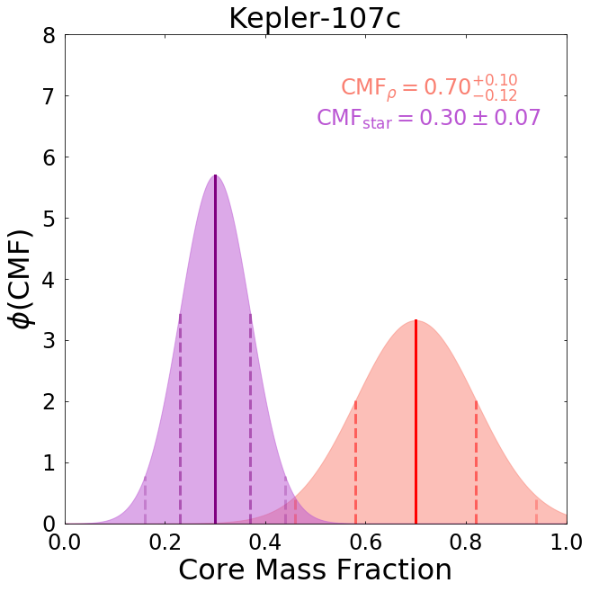
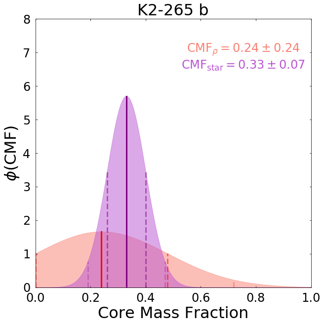
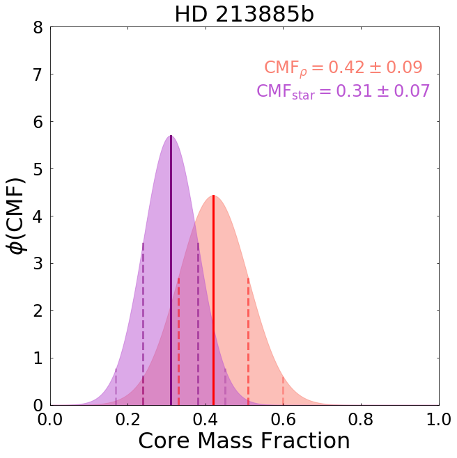
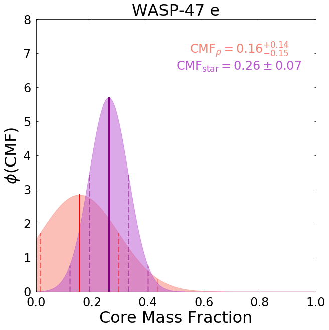
Figure 1: Probability density functions ($\phi$) as a function of core mass fraction given 1$\sigma$ distributions for CMF_ρ (red) and CMF_star (purple). All CMF calculations assume that the cores are pure iron and silicate mantles are iron-free, such that CMFs with these assumptions are equivalent to iron mass fraction. Figures are as listed in Table 1, in order of increasing radius.

Planet	CMFρ	CMFstar	$P(\mathcal{H}^{0})$ (%)	1$\sigma$ Class	2$\sigma$ Class
K2-229 b	$0.565^{+0.16}_{-0.20}$	$0.29\pm 0.06$	42	IHS	IHS
HD 219134 c	$0.42^{+0.13}_{-0.14}$	$0.28\pm 0.09$	70	IHS	IHS
Kepler-10 b	$0.13^{+0.15}_{-0.13}$	$0.28\pm 0.05$	65	IHS	IHS
HD 219134 b	$0.29\pm 0.15$	$0.28\pm 0.09$	100	IHS	IHS
Kepler-107 c	$0.70^{+0.10}_{-0.12}$	$0.30\pm 0.07$	1	SM	SM
HD 15337 b	$0.34\pm 0.15$	$0.29\pm 0.07$	96	IHS	IHS
K2-265 b	$0.24\pm 0.24$	$0.33\pm 0.07$	94	IHS	IHS
HD 213885 b	$0.42\pm 0.09$	$0.31\pm 0.07$	66	IHS	IHS
WASP-47 e	$0.155^{+0.14}_{-0.15}$	$0.26\pm 0.07$	80	IHS	IHS
Kepler-20 b	$0.26^{+0.14}_{-0.16}$	$0.30\pm 0.10$	98	IHS	IHS
55 Cnc e	$0.004^{+0.10}_{<0}$	$0.31\pm 0.10$	9	LDSP	IHS

Table 2: Inferred properties of the selected small, well-characterized exoplanets in order of increasing radius. IHS: Indistinguishable from Host Star, SM: super-Mercury, or LDSP: Low-Density Small Planet. While we classify planets at the $1\sigma$ level, we only consider planets that deviate from their host stars at the $2\sigma$ level to be conclusively inconsistent with the null hypothesis. The CMF_ρ and $P(\mathcal{H}^{0})$ values from earlier published M and R are in Table S3. Planets are listed in order of increasing radius as in Table 1.

6 Cases for a Rejected Null Hypothesis

For planets that deviate from $\mathcal{H}^{0}$ in Table 2, there are two cases, (1) in which CMF_star $<$ CMF_ρ, suggesting a planet with a larger core than expected, a super-Mercury, and (2) in which CMF_star $>$ CMF_ρ, a low-density small planet, which then suggests a region of non-unique solutions. We define and use the term Low-Density Small Planet (LDSP) for planets with an apparent density deficit, but distinguished from super-Puffs, a class of super-Earth mass planets with gas-giant transit radii leading to bulk densities of $\lesssim 0.1$ g/cc (e.g., Wang & Dai, 2019, and references therein). In contrast, LDSPs have bulk densities that can only be explained with a rock-dominated composition but sufficiently low that they are inconsistent with $\mathcal{H}^{0}$. For example, the candidate LDSP 55 Cnc e has a mean bulk density of $\sim 6.25$ g/cc which, for its mass, is consistent with a rocky (pure MgSiO₃) composition, but is $\sim 1.76$ g/cc lower than its expected bulk density per $\mathcal{H}^{0}$.

Kepler-107 c and 55 Cnc e, the two planets inconsistent with $\mathcal{H}^{0}$ at $>$ 1$\sigma$ level, differ in that Kepler 107c has a mass excess relative to what would be predicted by its host star, while 55 Cnc e has a relative mass deficit. This demands multiple explanations for these planets and suggests a diversity of planetary outcomes for planets that orbit close to their stars.

6.1 Super-Mercuries

Kepler-107c has a greater core mass fraction than predicted by its host star’s Fe/Mg abundances. There are few explanations for increasing the density of a planet beyond excess iron relative to MgO and SiO₂. The simplifying assumption of a solid, pure iron core means that $P(\mathcal{H}^{0}$) is an upper bound. Therefore, this planet is likely a super-Mercury.

Considering the actual core properties of the rocky solar system planets, it is likely that the cores of exoplanets contain some amount of alloying light elements and are at least partially liquid. The cores of the terrestrial solar system planets contain $\sim$ 10% light elements and are volumetrically dominated by liquid (e.g., Helffrich, 2017; Smith et al., 2012; Aitta, 2012; Birch, 1952; Lehmann, 1936). Including these factors only strengthens the case for a large core for Kepler-107c.

Both light element incorporation and liquid iron reduce the density of the core. For models that conserve both mass and radius, our simplifying assumption of overestimating the core density underestimates core volume due to systematically bounding the density as a likely maximum. CMF_ρ values assuming a pure and solid Fe core are $\sim$ 0.02-0.04 lower than the liquid and light-element-enriched core cases for a given planetary mass and radius. As an example, assuming a liquid core for K2-229 b, the second most probable super-Mercury, increases CMF_ρ by $\sim$0.02 relative to a solid core, corresponding to a 5% decrease in $P(\mathcal{H}^{0})$.

An additional assumption is that all iron is in the core and none in the mantle. In the calculation of CMF_star, Fe/Mg is constant, but the oxidation of iron removes Fe from the core as well as adds oxygen to the planet, decreasing the effective CMF_star by 0.02-0.03 compared to the FeO-free case. The comparable CMF_ρ calculation, however, oxidizes Fe from the core incorporating it into the mantle as FeO. This increases the average density of the mantle while decreasing the density of the planet through added oxygen, decreased compressibility of the oxide compared to the metal, and decreased core mass. For example, an Earth-like, whole-rock assemblage has 4 mol % FeO, accounting for oxidation of 13 mol% of Earth’s iron, has a bulk modulus of  250 GPa (Lee et al., 2004), while the bulk modulus of solid, hcp iron is 178 GPa (Smith et al., 2018). As a result, the simplifying assumption that all iron is in the core, a resulting model for CMF_ρ at a given mass and radius is an underestimate for planet iron fraction by $\sim$ 0.01-0.04. For example, the assumption of a Fe-free mantle in K2-229 b predicts CMF${}_{\rho}=0.565$. 10 mol% oxidation of the available iron, removing it from the core and incorporating it into the mantle as an iron oxide, requires a 0.032 increase in planet Fe/Mg for K2-229 b at its given mass to reproduce this planet’s radius. Given constant stellar Fe/Mg, this increase in iron corresponds to an 8% decrease in $P(\mathcal{H}^{0})$ relative to the Fe-free mantle case.

For both assumptions of a solid, pure iron core and iron-free mantle, the probability assigned to $\mathcal{H}^{0}$ is an upper bound in the case CMF_ρ $>$ CMF_star, and, therefore, the 5% probability criterion for super-Mercuries in this situation is a conservative measure.

6.2 Low-Density Small Planets

Four compositional variations can potentially explain LDSPs, (1) significant oxidization of iron such that it is removed from the core and incorporated into the mantle (e.g. Rogers & Seager (2010)), (2) a calcium-aluminum oxide dominated planet that formed from only these highest-temperature refractory materials with significantly depleted Fe (e.g. Dorn et al. (2019)), (3) volatile outer layers (e.g. Ehrenreich et al. (2012); Crida et al. (2018); Tsiaras et al. (2016); Angelo & Hu (2017b); Dorn et al. (2017)), or (4) or significant melt fraction (Bower et al., 2019).

As with the impact of oxidation on K2-229 b, we explore the degree to which core oxidation affects our analysis of the null hypothesis in the case of LDSPs. In the case that 55 Cnc e is core-free due to oxidation of all iron, $P(\mathcal{H}^{0})$ increases from 9% to 10% (Fig. 2). As in 6.1, this is a consequence of the iron being incorporated in a lower density, lower compressibility oxide as compared to the metal. At the same time, this results in an associated decrease in CMF_star due to an added oxygen atom per iron atom.

A major objection to the possibility of a planet made of ultra-high temperature condensates as proposed by Dorn et al. (2019) is that there is an insufficient mass of Al and Ca present within the protoplanetary disk available to produce the observed masses of these planets. For instance, reproducing the mass of 55 Cnc e assuming it formed from a minimum mass solar nebula Kuchner (2004), which likely overestimates the disk mass available to planets forming around its K-dwarf host, requires a factor of $\sim$3.5 (0.55 dex) and $\sim$2 (0.3 dex) increase in the already super-solar Ca and Al abundances of 55 Cnc, respectively. That being said, the mean density of 55 Cnc e is consistent with a virtually iron-free planet of MgSiO₃, similar to the compositional prediction in this hypothesis.

Where the lower-than-expected density cannot be explained by oxidation or iron deficit, the most likely explanation is a combination of H/He or higher-mass atmospheric compositions including H₂O and CO₂ (e.g. Ehrenreich et al. (2012); Crida et al. (2018); Tsiaras et al. (2016); Angelo & Hu (2017b); Dorn et al. (2017)). For 55 Cnc e, the radius deficit between what is observed and what is expected per $\mathcal{H}^{0}$ can be explained by a $\sim 1000$ km thick atmosphere. Given the proximity of 55 Cnc e to its host, an H/He or H₂O-dominated atmosphere would result in escaping hydrogen which has not been observed (e.g., Bourrier et al., 2018, and references therein). A water-rich atmosphere has recently been ruled out at the 3$\sigma$ level (Jindal et al., 2020): If 55 Cnc e does have an atmosphere, it must be dominated by heavier species including CO, CO₂, or N₂.

We note that earlier, larger, measurements of the radius of 55 Cnc e and WASP-47e place these planets as inconsistent with $\mathcal{H}^{0}$ at greater than 2$\sigma$ and 1$\sigma$ level, respectively (Table S3), which would predict both planets as LDSPs. Both planet radii have been revised downward using updated stellar parameters from Gaia parallaxes (Dai et al. (2019)).

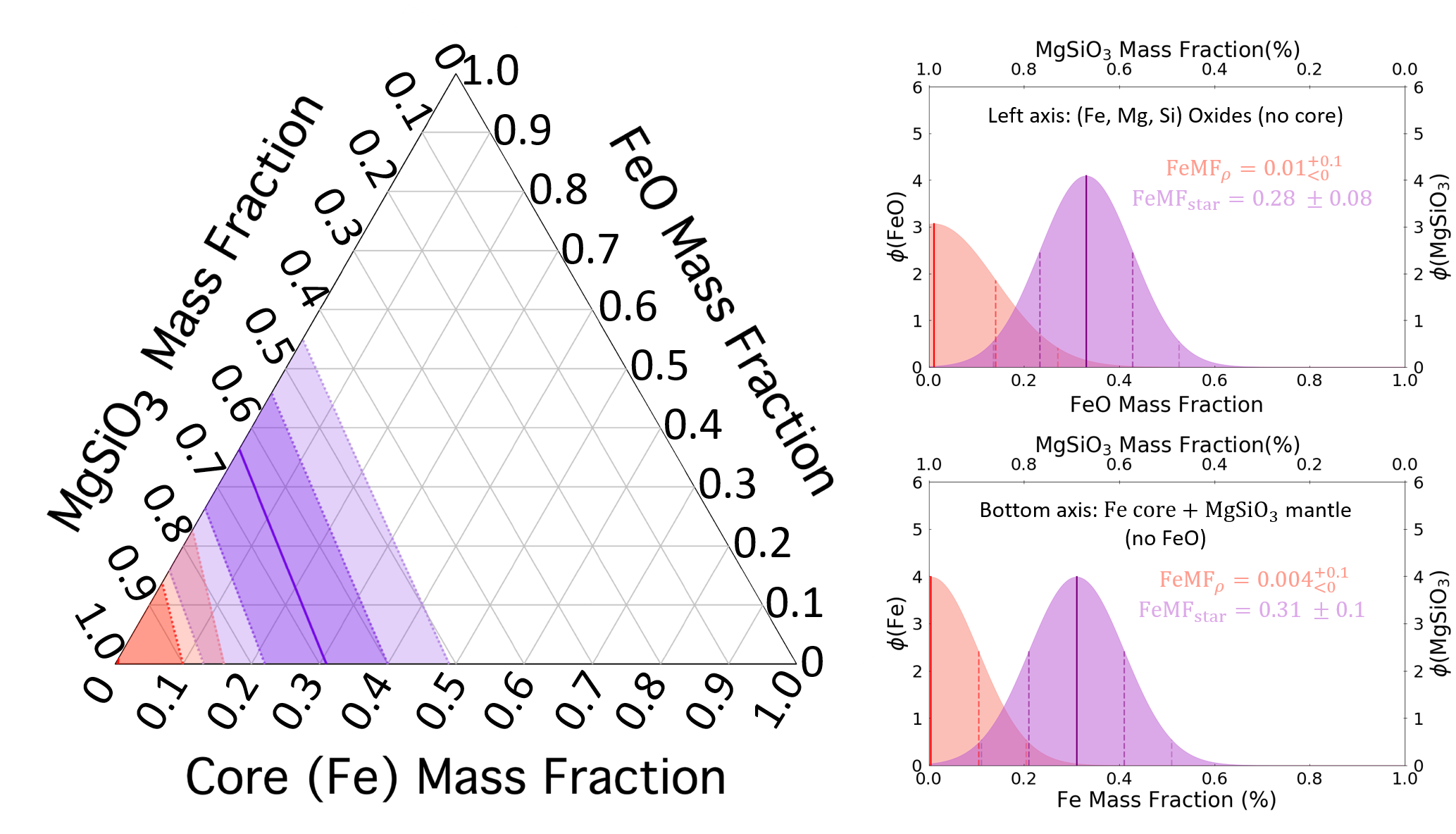
Figure 2: Ternary diagram of the CMF-MMF-FeO solution space for 55 Cnc e. All possible CMF_star solutions (purple, dark 1$\sigma$, light 2$\sigma$) and CMF_ρ solutions (red, dark 1$\sigma$, light 2$\sigma$) are plotted with the constraint that CMF+MgSiO₃+FeO $=100\%$. Our model assumes that the core is pure Fe, and all (Fe, Mg, Si) oxides reside in the mantle. FeMF_ρ and FeMF_star refer to the bulk Fe mass fraction inferred from mass-radius measurements and host-star abundances, respectively. In the case of no oxidation, FeMF_ρ = CMF_ρ and FeMF_star = CMF_star.

6.3 Necessary Observational Improvements to Reject the Null Hypothesis

Current efforts are underway to improve mass and radius measurements for rocky exoplanets. We investigate here the needed improvements in the observational uncertainties of mass, radius, and host-star abundances to help quantify the range of rocky planet compositions. We find that increasing precision in planetary radius measurements is the most critical.

Across the radius and mass range of the analysis (2.5-9.7 $M_{\oplus}$ and 1.1-1.9 $R_{\oplus}$), we calculate the relative effects of uncertainties in measured mass, radius, and stellar abundances in CMF_ρ and CMF_star (Figure 3). Uncertainties arising in mass and/or radius resulting from the uncertainties in the underlying equation of states for each layer are minimal (Unterborn & Panero, 2019). The uncertainty in CMF_ρ is weakly dependent upon the planetary mean density in the considered range (Table S1).

For a typical planet with CMF_ρ = 0.35, we determine that a 20% uncertainty in mass for a planet leads to a CMF_ρ uncertainty of 0.15 (Figure 3a, Table S1). The observational uncertainties in planet radius have the greatest impact on inferred CMF_ρ. A 10% radius uncertainty, again for a typical CMF_ρ of 0.35, leads to an uncertainty that is as large as the central value, i.e. CMF = 0.35 $\pm$ 0.35.

The observational uncertainty in host-star Fe, Mg, and Si abundances have a proportionally smaller effect on CMF_star (Table S2). A 40% uncertainty in molar Fe/Mg leads to a CMF_star uncertainty $<$ 0.10 (Figure 3b). We find that the uncertainty in molar Si/Mg has minimal impact.

Improving mass and radius uncertainties for small planets is a resource-intensive process, which will benefit from increased signal-to-noise ratios of TESS (Ricker et al., 2015) and CHEOPS (Benz et al., 2018) for bright hosts, along with parallax measurements from Gaia (Gaia Collaboration et al., 2016), which may improve mean planet density observational uncertainty to as little as 4% (Stevens et al., 2018). From the stellar perspective, direct analysis for [Fe/Mg] and [Si/Mg], circumvents compounding effects of covariances and permits for a reduction in uncertainties relative to calculating abundances from [Fe/H], [Mg/H], and [Si/H] (Epstein et al., 2010).

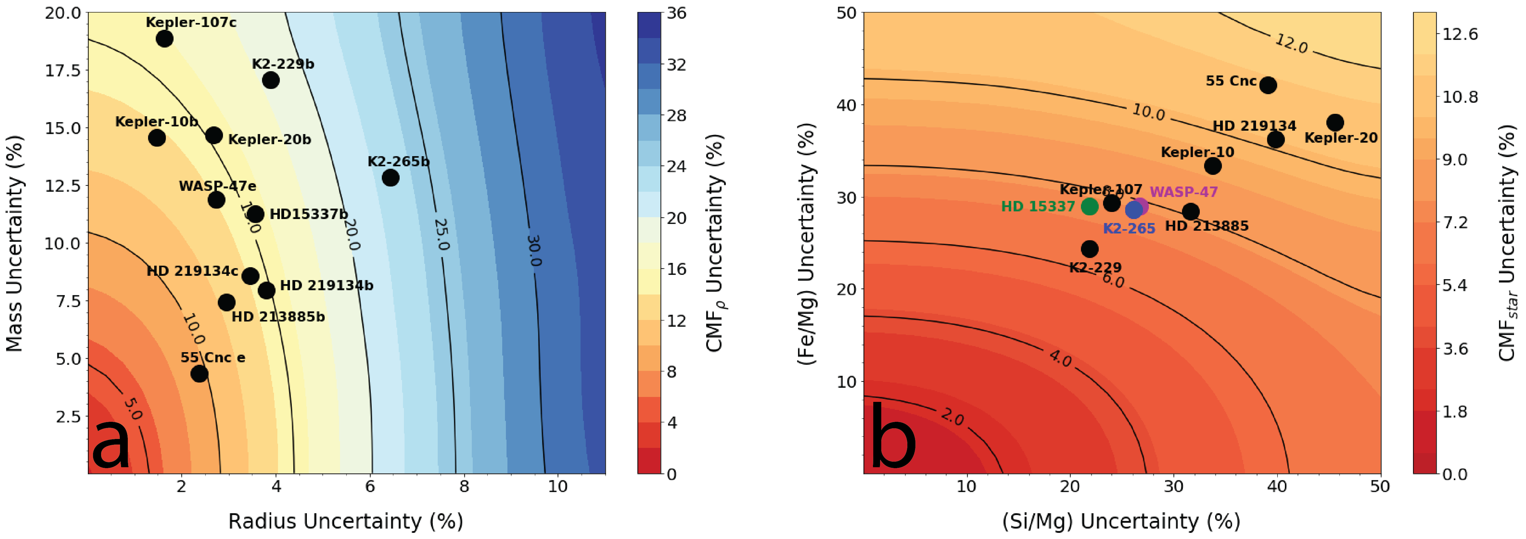
Figure 3: (a) Uncertainty in CMF_ρ as a function of planet mass and radius uncertainties. Uncertainties here assume $M_{p}=5.0M_{\oplus}$ and $R_{p}=1.545R_{\oplus}$ for a central value for CMF_ρ=0.35. Values in Table 2 are exact. (b) Uncertainty in CMF_star as a function of uncertainties in the stellar, molar Fe/Mg and Si/Mg. We plot uncertainties for central values of Fe/Mg = 0.98 and Si/Mg = 1.0 which result in a central value of 0.35 for CMF_star. HD 15337, K2-265, and WASP-47 are colored for clarity.

Assuming a near best-case precision of 4% in mass, 1% in radius (5% $\rho$ uncertainty), and 8% in Fe/Mg and Si/Mg stellar abundances (corresponding to $\sim$ solar Fe/Mg and Si/Mg uncertainties), for planets in the range of 2.5-9.7 $M_{\oplus}$ and 1.1-1.9 $R_{\oplus}$, the null hypothesis cannot be refuted when 0.5 $<$ CMF_ρ/CMF_star $<$ 1.4. For the planets in our sample set, assuming accurate central values for each measurement, Kepler-10b and 55 Cnc e may be conclusively determined to have lower-than-expected densities, while HD 219134c and K2-229 b may be sufficiently resolved as planets with greater-than-expected densities, or super-Mercuries (Fig. 4, Table S4). The remaining planets, HD 219134 b, K2-265b, WASP-47e, HD 15337 b, HD 213885b, and Kepler 20b cannot be distinguished from the null hypothesis at the 2$\sigma$ level using mass, radius, and stellar abundances.

Next, we consider Mercury, Earth, Mars. While these planets are smaller than those in our sample, their geophysical constraints on CMF provide test cases for the validity of our methods and assumptions. MESSENGER constrained Mercury’s CMF to $\sim 0.69-{}0.77$, corresponding to CMF_ρ/CMF${}_{\mathrm{star}}=2.17-2.43$ (Nittler et al., 2019). Were Mercury to be viewed as an exoplanet with near-best case observation precisions, it should, therefore, be resolvable as denser than expected. Applying the methods and assumptions outlined in this work, we indeed find Mercury would be resolvable as denser than expected with CMF_ρ/CMF${}_{\mathrm{star}}=1.92$ and $P(\mathcal{H}^{0})$ indistinguishable from zero. Earth has a CMF_ρ/CMF_star of 1.02 (McDonough, 2017, and references therein). Thus, even with best-case observational precisions, the Earth as an exoplanet would be indistinguishable from the Sun. Using our approach on Earth, we find CMF_ρ/CMF_star = 1.03 and $P(\mathcal{H}^{0})$ = 99%. Last, while Mars has a molar Fe/Mg ratio to within $\sim 10-{}15\%$ of the Sun’s, much of its Fe is oxidized, leading to a smaller CMF than the Earth. Geophysical constraints give CMF_ρ/CMF${}_{\mathrm{star}}\sim 0.57-0.67$ for Mars. Thus, even with significant oxidation of iron, Mars as an exoplanet should still be indistinguishable from the Sun at the 2$\sigma$ level. Our approach suggest values on the lower end without iron oxidation, CMF_ρ/CMF_star = 0.57 and $P(\mathcal{H}^{0})$ = 11% (Wanke & Dreibus, 1994; Bertka & Fei, 1998; Zharkov & Gudkova, 2005; Yoshizaki & McDonough, 2020).

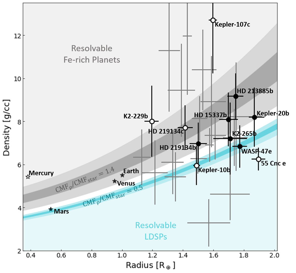
Figure 4: Planet density as a function of radius for the 11 planets in our sample (circles) and the solar system terrestrial planets (stars). The observational radius and density uncertainties are plotted for each planet. Open circles indicate planets that may be distinguishable from $\mathcal{H}^{0}$ at the 2$\sigma$ significance level should $\sigma_{M_{p}}=4\%$, $\sigma_{R_{p}}=1\%$, and $\sigma_{\mathrm{Fe/Mg}}=8\%$ precisions be attained. The dark-gray shaded region covers the density range of our sample for which $\mathrm{CMF_{\rho}}$/$\mathrm{CMF_{star}}$ = 1.4, while the light gray shading reflects the middle 95% range of $\mathrm{CMF_{star}}$ from the stellar abundances in the Hypatia catalog. Similarly, the cyan shading reflects the range of this sample and of the equivalent Hypatia range where $\mathrm{CMF_{\rho}}$/$\mathrm{CMF_{star}}$ = 0.5. Gray crosses are the 17 planets that meet our mass and radius criteria but lack Fe, Mg, and Si abundances measurements of their host stars. These planets are listed in Table S5.

7 Discussion and Conclusions

We assess the statistical consistency of a planet’s composition and structure as inferred from its mass and radius with what is expected from its host’s major rock-building elemental abundance ratios. We test the hypothesis directly and demonstrate that for just one planet, Kepler 107c, the mass and radius cannot be described as a terrestrial planet with the same relative major rock-building element abundances as its host, demanding a two-fold excess of iron. This approach is complementary to the Bayesian approach in Dorn et al. (2015) and Otegi et al. (2020), which leverage stellar abundances to reduce planetary structure degeneracy, in which the null hypothesis tested here is assumed a priori. Once the conditions under which a terrestrial planet is describable by its host’s abundances are understood, a more complete Bayesian analysis of planetary composition and structure will be warranted.

We demonstrate that super-Mercuries with an iron overabundance that is at least 40% greater than CMF_star may be resolvable as having different from host-star major rock-building element compositions. For example, we show that HD 219134c will be a resolvable super-Mercury while HD 213885b will remain unresolvable despite these planets having the same mean $\mathrm{CMF}_{\rho}$. The difference arises from HD 213885 being more Fe-rich relative to silicates than HD 219134 leading to 135% and 150% iron overabundances for HD 213885b and HD 219134b, respectively.

Several planetary formation and evolution mechanisms may explain super-Mercury planets. Each model identifies mechanisms by which planets are enriched in iron relative to their host star. These models include giant impacts (Leinhardt & Stewart, 2011; Marcus et al., 2010), a series of smaller impacts (Chau et al., 2018; Swain et al., 2019), mantle evaporation of hot planets (e.g., Santerne et al., 2018, and references therein), iron-enrichment in the inner regions of planet-forming disks due to iron condensing at a higher temperature than silicate material (Lewis, 1972) or via photophoresis (e.g., Ebel & Stewart, 2019, and references therein), and mantle stripping via planet-star tidal interactions (Jia & Spruit, 2016) or planet-planet tidal interactions (Deng, 2020). Each model to explain the formation of Mercury or super-Mercuries involves compositional sculpting of such planets relative to their host star. The frequency and orbital properties of exo-super-Mercuries are a crucial test of these theories.

HD 219134c is potentially resolvable as a super-Mercury only when analyzed relative to its host’s abundances. HD219134 is a star with proportionally little Fe with Fe/Mg = 0.69 $\pm$ 0.25, yet slightly iron-enriched relative to Solar, with [Fe/H] = 0.09 (Hinkel et al., 2014). Had the planetary structure analysis focused solely on the CMF_ρ ($0.42^{+0.13}_{-0.14}$), this planet may have been missed as a planet that underwent significant chemical sculpting, as it is less than 1$\sigma$ greater than an Earth-like CMF of 0.32. Notably, this planet orbits outside that of HD 219134 b, which is indistinguishable from its host star. Similarly, K2-229 b may have been prematurely misidentified as a super-Mercury, even with the updated mass and radius values used in this study, had its host star’s abundances not been considered. K2-229 b and HD 219134 c show that stellar major rock-building element composition must be carefully considered when investigating the outcome diversity of rocky planet formation to avoid failing to or misidentifying a planet as a super-Mercury or LDSP.

We also show that we can identify low-density, small planets whose CMF_ρ is 50% than predicted by CMF_star. The source of the low density is degenerate, but the 1$\sigma$ mass deficit for 55 Cnc e cannot be explained through oxidation of all iron. The relative influence of atmospheric layers, a dramatic iron deficit, or global magma oceans remain degenerate. Such planets offer important clues as to planetary system evolution, demonstrating that small planets below the radius gap cannot be exclusively rocky planets.

The approach of comparing expected density based on host-star composition to that of the planet only addresses the most extreme cases of compositional sculpting. The remaining planets in the sample set, more than half, are not distinguishable from the null hypothesis, nor will they be distinguishable from their host star with respect to composition based on mass and radius measurements alone. For potential LDSPs, further constraint on the differences between host-star composition and rocky planet composition must come from alternate methods. First, the measurement of day-to-night side temperature contrast could reveal a thick atmosphere and thus a LDSP (Koll et al., 2019). Second, the measurement of planet atmospheric composition and relative abundance ratio (Morley et al., 2017) can be compared to that of the host star.

Plotnykov & Valencia (2020) and Scora et al. (2020) have recently presented complementary approaches to detecting rocky planets with non-stellar compositions. Plotnykov & Valencia (2020) compare the mean planetary CMF distribution ($\langle\mathrm{CMF}_{\rho}\rangle$) for likely rocky planets with $\mathrm{\sigma_{M_{p}}}$ and $\mathrm{\sigma_{R_{p}}}$ $<$ 25% to the mean stellar CMF distribution ($\langle\mathrm{CMF_{star}}\rangle$) of the stars in the Hypatia Catalog (Hinkel et al., 2014). The authors find that the $\mathrm{CMF}_{\rho}$ distribution peaks at a lower value and is more broad than the $\mathrm{CMF_{star}}$ distribution, requiring an explanation in planet formation theories. Scora et al. (2020) investigate whether the diversity of $\langle\mathrm{CMF}_{\rho}\rangle$ relative to what is expected from $\langle\mathrm{CMF_{star}}\rangle$ can be explained through the cumulative effects of collisions during formation, finding that collisions alone cannot explain the diversity of rocky planet compositions.

While comparing statistical average values for CMF_ρ and $\mathrm{CMF_{star}}$ is useful for assessing planets in which no stellar abundance measurements are made, it fails to consider the composition deviation in Fe/Mg from star to planet on an individual basis. Assuming a best case CMF_ρ uncertainty of 0.03 (Kepler-107c Table S4) and $\langle\mathrm{CMF_{star}}\rangle\;=0.32^{+0.14}_{-0.12}$ (Plotnykov & Valencia, 2020), only planets with CMF${}_{\rho}<0.02$ or $>0.67$ (ratios of $<0.06$ and $>2.1$, respectively) may be resolvable as statistically inconsistent with $\langle\mathrm{CMF_{star}}\rangle$. As observational precisions increase and Fe/Mg and Si/Mg values become more widely reported, our approach will be able to identify these same compositional extremes and more modest cases of compositional sculpting.

To assess the formation processes that result in measurable compositional deviations for planets smaller than the radius gap will require a larger, more precise sample with both extreme and more moderate cases of compositional sculpting. In our sample selection process, we identified 17 small planets with high-precision mass and radius measurements, but without host-star abundance measurements beyond [Fe/H] (Table S5). The sample-set, therefore, may be doubled rapidly with targeted, high-precision stellar abundance analysis. With a larger data set, deviations from the expected can be addressed statistically much like the radius populations are able to do now. It is imperative that host-star Fe, Mg, and Si abundance measurements are included along with mass and radius measurements of likely rocky planets as part of the discussion and inference on their structure and composition. Without mass-radius and host-star abundance measurements, it is impossible to determine if a planet’s composition reflects that of its host and, in turn, determine its most likely formation pathways.

Supplementary Information and Supporting Data

Calculation of CMF and $\sigma_{\text{CMF}}$

CMF_ρ, CMF_star, and their uncertainties are calculated based on planetary mass, radius, host-star Fe/Mg and Si/Mg as well as the uncertainty in each parameters. Example models in Table S1 and S2 were calculated using ExoLens, an open-source compositional calculator for rocky planets based on ExoPlex. This calculator estimates the core mass fractions, CMF_ρ, CMF_star, and their uncertainties of a 0.1-10$M_{\oplus}$ planet from mass and radius to within 1-2% of ExoPlex, automatically calculating $P(\mathcal{H}^{0})$. ExoLens is available at the GitHub (https://github.com/schulze61/ExoLens).

Mp	$\sigma_{M_{p}}$ ($\%$)	Rp	$\sigma_{R_{p}}$ ($\%$)	CMFρ	$\sigma_{\text{CMF}_{\rho},upper}$	$\sigma_{\text{CMF}_{\rho},lower}$
5	10	1.54	1	0.35	0.09	0.10
5	10	1.54	2.5	0.35	0.12	0.13
5	10	1.54	10	0.35	0.32	0.39
5	5	1.54	5	0.35	0.17	0.19
5	10	1.54	5	0.35	0.18	0.20
5	20	1.54	5	0.35	0.22	0.28
1	10	0.99	5	0.35	0.19	0.22
2.5	10	1.28	5	0.35	0.19	0.21
7.5	10	1.71	5	0.35	0.18	0.20
10	10	1.84	5	0.35	0.17	0.20
5	10	1.65	5	0.10	0.22	$>$0.10
5	10	1.59	5	0.25	0.20	0.22
5	10	1.50	5	0.45	0.17	0.19
5	10	1.37	5	0.70	0.13	0.14
5	10	1.25	5	0.90	0.10	0.11

Table S1: The effects of $M_{p}$, $R_{p}$, $\sigma_{R_{p}}$ and $\sigma_{M_{p}}$ on CMF_ρ and $\sigma_{\text{CMF}_{\rho}}$.

Fe/Mg	$\sigma_{\mathrm{Fe/Mg}}$ ($\%$)	Si/Mg	$\sigma_{\mathrm{Si/Mg}}$ ($\%$)	CMFstar	$\sigma_{\text{CMF}_{\mathrm{star}}}$
1.0	20	1.0	10	0.36	0.05
1.0	20	1.0	20	0.36	0.05
1.0	20	1.0	30	0.36	0.06
1.0	20	1.0	40	0.36	0.07
1.0	20	1.0	50	0.36	0.09
1.0	20	0.5	20	0.44	0.05
1.0	20	0.8	20	0.39	0.05
1.0	20	1.25	20	0.33	0.05
1.0	20	2.0	20	0.26	0.05
1.0	10	1.0	20	0.36	0.04
1.0	30	1.0	20	0.36	0.07
1.0	40	1.0	20	0.36	0.10
1.0	50	1.0	20	0.36	0.12
0.5	20	1.0	20	0.22	0.04
0.8	20	1.0	20	0.31	0.07
1.25	20	1.0	20	0.41	0.10
2.0	20	1.0	20	0.53	0.12

Table S2: The effects of Fe/Mg, Si/Mg, $\sigma_{\mathrm{Fe/Mg}}$ and $\sigma_{\mathrm{Si/Mg}}$ on $\mathrm{CMF_{\star}}$ and $\sigma_{\text{CMF}_{\mathrm{star}}}$.

Previous studies

We calculate CMF_ρ estimates for planets in our sample with multiple reported mass and radius measurements on NASA Exoplanet Archive. We only consider studies where both mass and radius, and thus bulk density, are measured. All CMF_ρ values presented here are calculated using ExoLens.

Planet	Rp [$R_{\oplus}$]	Mp [$M_{\oplus}$]	Source	CMFρ	$P(\mathcal{H}^{0})$ (%)
K2-229 b	$1.164^{+0.066}_{-0.048}$	$2.59\pm 0.43$	Santerne et al. (2018)	$0.68^{+0.15}_{-0.18}$	13
HD 219134 c	$1.511\pm 0.047$	$4.36\pm 0.22$	Gillon et al. (2017)	$0.30^{+0.12}_{-0.13}$	99
Kepler-10 b	$1.481^{+0.049}_{-0.029}$	$4.61^{+1.27}_{-1.26}$	Esteves et al. (2015)	$0.42^{+0.21}_{-0.35}$	90
	$1.47\pm 0.03$	$3.33\pm 0.49$	Dumusque et al. (2014)	$0.12^{+0.17}_{<0}$	74
	$1.46\pm 0.02$	$4.60\pm 1.26$	Fogtmann-Schulz et al. (2014)	$0.46^{+0.18}_{-0.30}$	81
	$1.416^{+0.033}_{-0.036}$	$4.56^{+1.17}_{-1.29}$	Batalha et al. (2011)	$0.55^{+0.17}_{-0.27}$	58
HD 219134 b	$1.602\pm 0.055$	$4.74\pm 0.19$	Gillon et al. (2017)	$0.15^{+0.14}_{-0.15}$	71
	$1.606\pm 0.086$	$4.36\pm 0.44$	Motalebi et al. (2015)	$0.05^{+0.24}_{<0}$	65
HD 15337 b	$1.64\pm 0.06$	$7.51^{+1.09}_{-1.01}$	Gandolfi et al. (2019)	$0.49^{+0.14}_{-0.16}$	48
WASP-47 e	$1.810\pm 0.027$	$6.83\pm 0.66$	Vanderburg et al. (2017)	$0.04^{+0.12}_{<0}$	24
	$1.82\pm 0.40$	$9.10^{+5.50}_{-3.60}$	Almenara et al. (2016)	$0.31^{+0.66}_{<0}$	100
	$1.817\pm 0.065$	$12.2\pm 3.7$	Dai et al. (2015)	$0.55^{+0.18}_{-0.29}$	62
Kepler-20 b	$1.91^{+0.12}_{-0.21}$	$8.7^{+2.1}_{-2.2}$	Gautier et al. (2012)	$0.08^{+0.39}_{<0}$	84
55 Cnc e	$1.947\pm 0.038$	$8.59\pm 0.43$	Crida et al. (2018)	$[<0,0.08]$	4
	$1.875\pm 0.029$	$7.99^{+0.32}_{-0.33}$	Bourrier et al. (2018)	$0.06^{+0.08}_{-0.08}$	14
	$1.91\pm 0.08$	$8.08\pm 0.31$	Demory et al. (2016c)	$0^{+0.18}$	31
	$2.173^{+0.097}_{-0.098}$	$8.37\pm 0.38$	Endl et al. (2012)	$<0$	0
	$2.08^{+0.16}_{-0.17}$	$7.81^{+0.58}_{-0.53}$	Demory et al. (2011)	$<0$	0
	$2.00\pm 0.14$	$8.63\pm 0.35$	Winn et al. (2011)	$[<0,0.17]$	40

Table S3: CMF_ρ values for previously reported mass and radius measurements in order of publication date.

Minimum Uncertainties

Planet	CMFρ	CMFstar	$\sigma_{\mathrm{Fe/Mg}}=\sigma_{\mathrm{Si/Mg}}$ (%)	$P(\mathcal{H}^{0})$ (%)	1$\sigma$ Class	2$\sigma$ Class
K2-229 b	$0.565^{+0.041}_{-0.043}$	$0.29\pm 0.06$	–	0.1	SM	SM
HD 219134 c	$0.42^{+0.05}_{-0.05}$	$0.28\pm 0.03$	14	5	SM	SM
Kepler-10 b	$0.13^{+0.06}_{-0.06}$	$0.28\pm 0.02$	9	5	LDSP	LDSP
HD 219134 b	$0.29^{+0.05}_{-0.05}$	$0.28\pm 0.02$	8	98	IHS	IHS
Kepler-107 c	$0.70^{+0.03}_{-0.03}$	$0.30\pm 0.07$	–	$\sim 0$	SM	SM
HD 15337 b	$0.34^{+0.05}_{-0.05}$	$0.29\pm 0.02$	8	69	IHS	IHS
K2-265 b	$0.24^{+0.04}_{-0.05}$	$0.33\pm 0.02$	8	13	LDSP	IHS
HD 213885 b	$0.42^{+0.04}_{-0.05}$	$0.31\pm 0.02$	8	12	SM	IHS
WASP-47 e	$0.155^{+0.056}_{-0.058}$	$0.26\pm 0.02$	8	21	LDSP	IHS
Kepler-20 b	$0.26^{+0.05}_{-0.05}$	$0.30\pm 0.01$	8	76	IHS	IHS
55 Cnc e	$0.004^{+0.06}_{<0}$	$0.31\pm 0.10$	–	3.4	LDSP	LDSP

Table S4: Minimum uncertainties needed to classify the planets in our sample at the 2$\sigma$ significance level. For these calculations, we assume $\sigma_{M_{p}}=4\%$ and $\sigma_{R_{p}}=1\%$. We vary $\sigma_{\mathrm{Fe/Mg}}=\sigma_{\mathrm{Si/Mg}}$ until $P(\mathcal{H}^{0})\leq 5\%$ stopping at the optimistic value of $\sigma_{\mathrm{Fe/Mg}}=\sigma_{\mathrm{Si/Mg}}=8\%$ if this $P(\mathcal{H}^{0})$ criteria is not met. For these planets, the $P(\mathcal{H}^{0})$ corresponding to $\sigma_{M_{p}}=4\%$, $\sigma_{R_{p}}=1\%$, and $\sigma_{\mathrm{Fe/Mg}}=\sigma_{\mathrm{Si/Mg}}=8\%$ is recorded. This stellar abundance criteria is derived from the recommended abundances of Lodders (2003). While such precisions will be difficult to obtain for extrasolar stars from spectroscopic abundance measurements alone, $\sigma_{\mathrm{Fe/Mg}}=\sigma_{\mathrm{Si/Mg}}=8\%$, nonetheless, provides a good stopping point for our minimum precision calculations. Planets with no value recorded in the abundance ratio uncertainty column do not require increased abundance precisions to classify at better than the 2$\sigma$ level if their mass and radius uncertainties reach 4% and 1%, respectively.

Calculating $P(\mathcal{H}^{0})$: Schematic for quantitative rejection of the null hypothesis

Figure S1: We illustrate the meaning of Equation (4) with an example of a planet whose CMF_ρ is similar to its CMF_star value (top) and one whose CMF_ρ is greater than its CMF_star value (bottom). The numerator of eqn. 4 computes the integral of the product of the distribution of each CMF value. In the case where they are similar, the overlaps are significant, yet where the CMF values are different, there is nearly no overlap. The denominator for each case accounts for the consequences of variable distribution widths so as to normalize the numerator to 1.

Figure 4 Planet Sample

Planet	Rp [$R_{\oplus}$]	Mp [$M_{\oplus}$]	M-R Source	P [days]	S.T.	Fe/Mg	Si/Mg	Spect. Source
K2-229 b	$1.197^{+0.045}_{-0.048}$ (3.9%)	$2.49^{+0.42}_{-0.43}$ (17.1%)	Dai et al. (2019)	0.58	G9	0.78$\pm$0.19	1.1$\pm$0.24	Santerne et al. (2018)
HD 219134 c	1.415$\pm$0.049 (3.5%)	3.96$\pm$0.34 (8.6%)	Ligi et al. (2019)	6.76	K3	0.69$\pm$0.25	0.98$\pm$ 0.39	Hypatia Catalog
Kepler-10 b	$1.489^{+0.023}_{-0.021}$ (1.5%)	$3.57^{+0.51}_{-0.53}$ (14.6%)	Dai et al. (2019)	0.84	G	0.62$\pm$0.14	0.83$\pm$0.16	Liu et al. (2016)
HD 219134 b	1.500$\pm$0.057 (3.8%)	4.27$\pm$0.34 (8.0%)	Ligi et al. (2019)	3.09	K3	0.69$\pm$0.25	0.98$\pm$ 0.39	Hypatia Catalog
Kepler-107 c	1.597$\pm$0.026 (18.9%)	9.39$\pm$1.77 (1.6%)	Bonomo et al. (2019)	4.9	G2	0.75$\pm$ 0.22	0.96$\pm$0.23	Bonomo et al. (2019)
HD 15337 b	$1.699^{+0.062}_{-0.059}$ (3.6%)	$7.20\pm 0.81$ (11.3%)	Dumusque et al. (2019)	4.76	K1	0.69$\pm$0.29	0.87$\pm$ 0.20	Hypatia Catalog
K2-265 b	$1.71\pm 0.11$ (6.4%)	$6.54\pm 0.84$ (12.8%)	Lam et al. (2018)	2.37	G8	0.84$\pm 0.24$	0.92$\pm 0.24$	Lam et al. (2018)
HD 213885 b	$1.745^{+0.051}_{-0.052}$ (3.0%)	$8.83^{+0.66}_{-0.65}$ (7.4%)	Espinoza et al. (2019)	1.008	G	0.81$\pm$0.23	0.98$\pm$0.31	Espinoza et al. (2019)
WASP-47 e	$1.773^{+0.049}_{-0.048}$ (2.7%)	$6.91^{+0.81}_{-0.83}$ (11.9%)	Dai et al. (2019)	0.79	G9	0.76$\pm$0.22	1.35$\pm$0.36	Hellier et al. (2012)
Kepler-20 b	$1.868^{+0.066}_{-0.034}$ (2.7%)	$9.70^{+1.41}_{-1.44}$ (14.7%)	Buchhave et al. (2016)	3.70	G8	0.71$\pm$0.27	0.90$\pm$0.41	Schuler et al. (2015)
55 Cnc e	$1.897^{+0.044}_{-0.046}$ (2.4%)	$7.74^{+0.37}_{-0.30}$ (4.3%)	Dai et al. (2019)	0.74	G8	0.76$\pm$ 0.32	0.87$\pm$0.34	Hypatia Catalog
GJ 1132 b	$1.130\pm 0.056$ (5.0%)	$1.66\pm 0.23$ (13.9%)	Bonfils et al. (2018)	1.63	M4.5	–	–	–
GJ 357 b	$1.217^{+0.084}_{-0.083}$ (6.9%)	$1.84\pm 0.31$ (16.9%)	Luque et al. (2019)	3.93	M2.5	–	–	–
LTT 3780 b	$1.332^{+0.072}_{-0.075}$ (5.5%)	$2.62^{+0.48}_{-0.46}$ (17.9%)	Cloutier et al. (2020a)	0.77	M4	–	–	–
Kepler-105 c	$1.31\pm 0.07$ (5.3%)	$4.60^{+0.92}_{-0.85}$ (19.2%)	Jontof-Hutter et al. (2016)	7.13	G1	–	–	–
L 98-59 c	$1.35\pm 0.07$ (5.2%)	$2.42^{+0.35}_{-0.34}$ (14.3%)	Cloutier et al. (2019)	3.69	M3	–	–	–
L 168-9 b	$1.39\pm 0.09$ (6.5%)	$4.60\pm 0.56$ (12.2%)	Astudillo-Defru et al. (2020)	1.40	M1	–	–	–
Kepler-406 b	$1.43\pm 0.03$ (2.1%)	$6.35\pm 1.4$ (22.1%)	Marcy et al. (2014)	2.43	G7	–	–	–
Kepler-36 b	$1.498^{+0.061}_{-0.049}$ (3.7%)	$3.83^{+0.11}_{-0.10}$ (2.7%)	Vissapragada et al. (2020)	13.87	G1	–	–	–
K2-141 b	$1.51\pm 0.05$ (3.3%)	$5.08\pm 0.41$ (8.1%)	Malavolta et al. (2018)	0.28	K7	–	–	–
Kepler-80 d	$1.53^{+0.09}_{-0.07}$ (5.2%)	$6.75^{+0.69}_{-0.51}$ (8.9%)	MacDonald et al. (2016)	3.07	K5	–	–	–
L 98-59 d	$1.57\pm 0.14$ (8.9%)	$2.31^{+0.46}_{-0.45}$ (19.7%)	Cloutier et al. (2019)	7.45	M3	–	–	–
GJ 9827 b	$1.577^{+0.027}_{-0.031}$ (1.8%)	$4.91\pm 0.49$ (10.0%)	Rice et al. (2019)	1.21	K5	–	–	–
K2-291 b	$1.589^{+0.095}_{-0.072}$ (5.3%)	$6.49\pm 1.16$ (17.9%)	Kosiarek et al. (2019)	2.23	G7	–	–	–
HD 80653 b	$1.613\pm 0.071$ (4.4%)	$5.60\pm 0.43$ (7.7%)	Frustagli et al. (2020)	0.72	K5	–	–	–
Kepler-60 b	$1.71\pm 0.13$ (7.6%)	$4.19^{+0.56}_{-0.52}$ (12.9%)	Jontof-Hutter et al. (2016)	7.13	G1	–	–	–
TOI-1235 b	$1.738^{+0.087}_{-0.076}$ (4.7%)	$6.91^{+0.75}_{-0.85}$ (11.6%)	Cloutier et al. (2020b)	3.45	M0.5	–	–	–
K2-216 b	$1.75^{+0.17}_{-0.10}$ (7.7%)	$8.0\pm 1.6$ (20%)	Persson et al. (2018)	2.17	K5	–	–	–

Table S5: Sample of well-characterized exoplanets including those without reported host star abundance measurements beyond [Fe/H] that otherwise meet our selection criteria. Host star elemental ratios Fe/Mg and Si/Mg are expressed as molar ratios. For each star, we derive molar ratios of Fe/Mg and Si/Mg using the solar abundances from Lodders et al. (2009). Planets with known host-star Fe/Mg and Si/Mg values are separated from those with unknown host Fe/Mg and Si/Mg via a horizontal line. Planets are listed in order of increasing radius within each of these subsets. S.T. = Spectral Type of the host star.

References

- Aitta (2012) Aitta, A. 2012, Icarus, 218, 967, doi: 10.1016/j.icarus.2012.01.007
- Almenara et al. (2016) Almenara, J. M., Díaz, R. F., Bonfils, X., & Udry, S. 2016, A&A, 595, L5, doi: 10.1051/0004-6361/201629770
- Angelo & Hu (2017a) Angelo, I., & Hu, R. 2017a, AJ, 154, 232, doi: 10.3847/1538-3881/aa9278
- Angelo & Hu (2017b) —. 2017b, AJ, 154, 232, doi: 10.3847/1538-3881/aa9278
- Astudillo-Defru et al. (2020) Astudillo-Defru, N., Cloutier, R., Wang, S. X., et al. 2020, A&A, 636, A58, doi: 10.1051/0004-6361/201937179
- Batalha et al. (2011) Batalha, N. M., Borucki, W. J., Bryson, S. T., et al. 2011, ApJ, 729, 27, doi: 10.1088/0004-637X/729/1/27
- Benz et al. (2018) Benz, W., Ehrenreich, D., & Isaak, K. 2018, CHEOPS: CHaracterizing ExOPlanets Satellite, 84, doi: 10.1007/978-3-319-55333-7_84
- Bertka & Fei (1998) Bertka, C. M., & Fei, Y. 1998, Earth and Planetary Science Letters, 157, 79, doi: 10.1016/S0012-821X(98)00030-2
- Birch (1952) Birch, F. 1952, J. Geophys. Res., 57, 227, doi: 10.1029/JZ057i002p00227
- Bonfils et al. (2018) Bonfils, X., Almenara, J. M., Cloutier, R., et al. 2018, A&A, 618, A142, doi: 10.1051/0004-6361/201731884
- Bonomo et al. (2019) Bonomo, A. S., Zeng, L., Damasso, M., et al. 2019, Nature Astronomy, 3, 416, doi: 10.1038/s41550-018-0684-9
- Bourrier et al. (2018) Bourrier, V., Dumusque, X., Dorn, C., et al. 2018, A&A, 619, A1, doi: 10.1051/0004-6361/201833154
- Bower et al. (2019) Bower, D. J., Kitzmann, D., Wolf, A. S., et al. 2019, A&A, 631, A103, doi: 10.1051/0004-6361/201935710
- Brugger et al. (2017) Brugger, B., Mousis, O., Deleuil, M., & Deschamps, F. 2017, ApJ, 850, 93, doi: 10.3847/1538-4357/aa965a
- Buchhave et al. (2016) Buchhave, L. A., Dressing, C. D., Dumusque, X., et al. 2016, AJ, 152, 160, doi: 10.3847/0004-6256/152/6/160
- Chau et al. (2018) Chau, A., Reinhardt, C., Helled, R., & Stadel, J. 2018, The Astrophysical Journal, 865, 35, doi: 10.3847/1538-4357/aad8b0
- Cloutier et al. (2019) Cloutier, R., Astudillo-Defru, N., Bonfils, X., et al. 2019, A&A, 629, A111, doi: 10.1051/0004-6361/201935957
- Cloutier et al. (2020a) Cloutier, R., Eastman, J. D., Rodriguez, J. E., et al. 2020a, AJ, 160, 3, doi: 10.3847/1538-3881/ab91c2
- Cloutier et al. (2020b) Cloutier, R., Rodriguez, J. E., Irwin, J., et al. 2020b, AJ, 160, 22, doi: 10.3847/1538-3881/ab9534
- Crida et al. (2018) Crida, A., Ligi, R., Dorn, C., Borsa, F., & Lebreton, Y. 2018, Research Notes of the American Astronomical Society, 2, 172, doi: 10.3847/2515-5172/aae1f6
- Crida et al. (2018) Crida, A., Ligi, R., Dorn, C., Borsa, F., & Lebreton, Y. 2018, Research Notes of the AAS, 2, 172, doi: 10.3847/2515-5172/aae1f6
- Crida et al. (2018) Crida, A., Ligi, R., Dorn, C., & Lebreton, Y. 2018, ApJ, 860, 122, doi: 10.3847/1538-4357/aabfe4
- Dai et al. (2019) Dai, F., Masuda, K., Winn, J. N., & Zeng, L. 2019, ApJ, 883, 79, doi: 10.3847/1538-4357/ab3a3b
- Dai et al. (2015) Dai, F., Winn, J. N., Arriagada, P., et al. 2015, ApJ, 813, L9, doi: 10.1088/2041-8205/813/1/L9
- Demory et al. (2016a) Demory, B.-O., Gillon, M., Madhusudhan, N., & Queloz, D. 2016a, MNRAS, 455, 2018, doi: 10.1093/mnras/stv2239
- Demory et al. (2011) Demory, B. O., Gillon, M., Deming, D., et al. 2011, A&A, 533, A114, doi: 10.1051/0004-6361/201117178
- Demory et al. (2016b) Demory, B.-O., Gillon, M., de Wit, J., et al. 2016b, Nature, 532, 207, doi: 10.1038/nature17169
- Demory et al. (2016c) —. 2016c, Nature, 532, 207, doi: 10.1038/nature17169
- Deng (2020) Deng, H. 2020, ApJ, 888, L1, doi: 10.3847/2041-8213/ab6084
- Dorn et al. (2019) Dorn, C., Harrison, J. H. D., Bonsor, A., & Hands, T. O. 2019, MNRAS, 484, 712, doi: 10.1093/mnras/sty3435
- Dorn et al. (2017) Dorn, C., Hinkel, N. R., & Venturini, J. 2017, A&A, 597, A38, doi: 10.1051/0004-6361/201628749
- Dorn et al. (2015) Dorn, C., Khan, A., Heng, K., et al. 2015, A&A, 577, A83, doi: 10.1051/0004-6361/201424915
- Dumusque et al. (2014) Dumusque, X., Bonomo, A. S., Haywood, R. D., et al. 2014, ApJ, 789, 154, doi: 10.1088/0004-637X/789/2/154
- Dumusque et al. (2019) Dumusque, X., Turner, O., Dorn, C., et al. 2019, A&A, 627, A43, doi: 10.1051/0004-6361/201935457
- Ebel & Stewart (2019) Ebel, D., & Stewart, S. 2019, in Mercury: The view after MESSENGER, ed. Solomon, S. C., Nittler, L. R., & Anderson, B. J. (Oxford: Cambridge University Press)
- Ehrenreich et al. (2012) Ehrenreich, D., Bourrier, V., Bonfils, X., et al. 2012, A&A, 547, A18, doi: 10.1051/0004-6361/201219981
- Elkins-Tanton & Seager (2008) Elkins-Tanton, L. T., & Seager, S. 2008, The Astrophysical Journal, 688, 628, doi: 10.1086/592316
- Endl et al. (2012) Endl, M., Robertson, P., Cochran, W. D., et al. 2012, ApJ, 759, 19, doi: 10.1088/0004-637X/759/1/19
- Epstein et al. (2010) Epstein, C. R., Johnson, J. A., Dong, S., et al. 2010, ApJ, 709, 447, doi: 10.1088/0004-637X/709/1/447
- Espinoza et al. (2019) Espinoza, N., Brahm, R., Henning, T., et al. 2019, MNRAS, 2769, doi: 10.1093/mnras/stz3150
- Esteves et al. (2015) Esteves, L. J., De Mooij, E. J. W., & Jayawardhana, R. 2015, ApJ, 804, 150, doi: 10.1088/0004-637X/804/2/150