FORTRESS II: FORTRAN programs for solving coupled Gross-Pitaevskii equations for spin-orbit coupled spin-2 Bose-Einstein condensate

Abstract

We provide here a set of three OpenMP parallelized FORTRAN 90/95 programs to compute the ground states and the dynamics of trapped spin-2 Bose-Einstein condensates (BECs) with anisotropic spin-orbit (SO) coupling by solving a set of five coupled Gross-Pitaevskii equations using a time-splitting Fourier spectral method. Depending on the nature of the problem, without any loss of generality, we have employed the Cartesian grid spanning either three-, two-, or one-dimensional space for numerical discretization. To illustrate the veracity of the package, wherever feasible, we have compared the numerical ground state solutions of the full mean-field model with those from the simplified scalar models. The two set of results show excellent agreement, in particular, through the equilibrium density profiles, energies and chemical potentials of the ground-states. We have also presented test results for OpenMP performance parameters like speedup and the efficiency of the three codes.

PROGRAM SUMMARY

Program Title: FORTRESS II
Licensing provisions: MIT
Programming language: (OpenMP) FORTRAN 90/95
Computer: Intel^® Xeon^® Platinum 8160 CPU @ 2.10GHz
Operating system: General
RAM: Will depend on array sizes.
Number of processors used: 8 processors for 1D code and 16 processors for 2D and 3D codes
External routines/libraries: FFTW 3.3.8 and Intel^® Math Kernel Library. The later is optional but gives better performance.
Journal reference of previous version: None
Nature of problem: To solve the coupled Gross-Pitaevskii equations for a spin-2 BEC with an anisotropic spin-orbit coupling.
Solution method: We use the time-splitting Fourier spectral method to split the coupled Gross-Pitaevskii equations into four sets of sub-equations. The resulting sub-equations are evolved in imaginary time to obtain the ground state of the system or in realtime to study the dynamics.

1 Introduction

The advent of optical traps in cold-atom experiments in the last couple of decades has made it possible to investigate the spinor Bose-Einstein condensates (BECs) in finer detail. A spinor BEC, a Bose-Einstein condensate with internal spin degrees of freedom was first realized with $f=1$ ²³Na atoms confined in an optical trap [1], where $f$ is the total spin per atom. Later, the different ground-state phases [2, 3] and spin dynamics of $f=2$ ⁸⁷Rb [4, 5, 6, 7] spinor BEC were also examined. In an optical trap, internal spin degrees of freedom of an atom representing $2f+1$ hyperfine sublevels corresponding to the spin projection quantum numbers $m_{f}=-f,-f+1,\ldots,+f$ are simultaneously trapped, which is an impossibility in magnetic traps. The interplay of the inter-atomic interactions and the Zeeman terms leads to a rich equilibrium phase-diagram for a spin-2 BEC [8]. Another feature of the spinor BECs distinguishing these from the scalar BECs is the spin-mixing dynamics [9]. One of the most crucial development in the last decade in the field of spinor BECs has been the experimental realization of spin-orbit (SO) coupling [10], thus paving the way for several novel studies in the field of spin-2 BECs [11, 12]. The theoretical proposals to realise SO coupling in spin-2 BECs have also been put forward [13].

In the absence of thermal and quantum fluctuations at $T=0$ K, the mean-field approximation allows one to describe an $f=2$ spinor BEC by a set of five-coupled nonlinear Gross-Pitaevskii equations (CGPEs) [14]. In general this coupled set of equations, termed as the mean-field model, is not analytically solvable without resorting to approximations. Thus there is a need for an efficient, robust, and flexible numerical tool which will aid the aforementioned studies. In this context, a wide range of numerical techniques have been employed in literature to study spinor BECs [15, 16, 17, 18]. In our earlier work [19], we developed a set of F90/95 codes to solve the mean-field model of SO-coupled $f=1$ spinor BEC with Rashba [20] SO coupling using time-splitting Fourier spectral method. In the present work, we discuss the Fourier-spectral method to solve the CGPEs for an SO-coupled spin-2 BEC, where the parts of Hamiltonian corresponding to spin-exchange collisions and SO coupling have to be numerically dealt with using a different numerical approach vis-à-vis a spin-1 BEC. To briefly summarize the method, we first split the CGPEs into four sub-sets of equations, where each set consists of five equations, using Lie operator splitting. The method then involves solving aforementioned four sets of equations one after the other over the same time interval with solution to each set serving as the input to the following set of equations. In the absence of SO coupling, we also develop two- and three-component scalar models which can be used to study the static properties of the system. These scalar models also serve an important purpose of validating the results obtained with the present set of codes where the SO coupling can be switched on/off by the user.

The program package consists of a set of three OpenMP parallelized FORTRAN 90/95 programs. This can be used to either (a) calculate stationary state solutions or (b) study dynamics of homogeneous or trapped SO-coupled spin-2 BECs, in three-dimensional (3D), quasi-two-dimensional (q2D), and quasi-one-dimensional (q1D) configurations. The two different objectives are accomplished by evolving the CGPEs either in imaginary or real time, respectively. We have provided the users the option of switching between these two modes within the codes.

The paper is organised as follows. In Sec. 2, we introduce the mean-field model of an SO-coupled spin-2 BEC. The scalar models which can be used to study a spin-2 BEC in the absence of SO coupling are described in Sec. 3. We describe the time-splitting spectral method to solve the CGPEs in Sec. 4, followed by the description of the three codes in Sec. 5. We present the test results for OpenMP performance in Sec. 6 and the numerical results in Sec. 7.

2 Coupled Gross-Pitaevskii equations for an SO-coupled spin-2 BEC-Mean-field model

The quantum and thermal fluctuations in an SO-coupled spin-2 BEC at $T=0$K can be neglected, and the system is very well described by the following set of coupled Gross-Pitaevskii equations (CGPEs) in dimensionless form [14, 20]

$$i\frac{\partial\phi_{\pm 2}({\bf x},t)}{\partial t} = \mathcal{H}\phi_{\pm 2}({\bf x},t)+\tau_{0}{\rho}({\bf x},t)\phi_{\pm 2}({\bf x},t)+\tau_{1}\{F_{\mp}({\bf x},t)\phi_{\pm 1}({\bf x},t)\pm 2F_{z}({\bf x},t)\phi_{\pm 2}({\bf x},t)\}$$ (1a)

$$+\tau_{2}\frac{\Theta({\bf x},t)\phi_{\mp 2}^{*}({\bf x},t)}{\sqrt{5}}+\Gamma_{\pm 2}({\bf x},t),$$

$$i\frac{\partial\phi_{\pm 1}({\bf x},t)}{\partial t} = \mathcal{H}\phi_{\pm 1}({\bf x},t)+\tau_{0}{\rho}({\bf x},t)\phi_{\pm 1}({\bf x},t)+\tau_{1}\left(\sqrt{\frac{3}{2}}F_{\mp}({\bf x},t)\phi_{0}({\bf x},t)+F_{\pm}({\bf x},t)\phi_{\pm 2}({\bf x},t)\right.$$ (1b)

$$\left.\pm F_{z}({\bf x},t)\phi_{\pm 1}({\bf x},t)\right)-\tau_{2}\frac{\Theta({\bf x},t)\phi_{\mp 1}^{*}({\bf x},t)}{\sqrt{5}}+\Gamma_{\pm 1}({\bf x},t),$$

$$i\frac{\partial\phi_{0}({\bf x},t)}{\partial t} = \mathcal{H}\phi_{0}({\bf x},t)+\tau_{0}{\rho}({\bf x},t)\phi_{0}({\bf x},t)+\tau_{1}{\sqrt{\frac{3}{2}}}\{F_{-}({\bf x},t)\phi_{-1}({\bf x},t)+F_{+}({\bf x},t)\phi_{1}({\bf x},t)\}$$ (1c)

$$+\tau_{2}\frac{\Theta({\bf x},t)\phi_{0}^{*}({\bf x},t)}{\sqrt{5}}+\Gamma_{0}({\bf x},t),$$

where, suppressing the explicit dependence of component wavefunctions $\phi_{j}$’s on ${\bf x}$ and $t$,

$$\mathcal{H} = -\frac{\mathbf{\nabla^{2}}}{2}+V(\mathbf{x})\quad\Theta=\frac{2\phi_{2}\phi_{-2}-2\phi_{1}\phi_{-1}+\phi_{0}^{2}}{\sqrt{5}},\quad F_{z}=\sum_{j=-2}^{2}j|\phi_{j}|^{2}$$

$$F_{-} = F_{+}^{*}=2\phi_{-2}^{*}\phi_{-1}+\sqrt{6}\phi_{-1}^{*}\phi_{0}+\sqrt{6}\phi_{0}^{*}\phi_{1}+2\phi_{2}\phi_{1}^{*},$$

and $\rho=\sum_{j=-2}^{2}|\phi_{j}|^{2}$ is the total density. In 3D, $\bf x$, Laplacian, trapping potential $V({\bf x})$, interaction parameters $(\tau_{0},\tau_{1},\tau_{2})$, and SO-coupling terms $\Gamma$’s are defined as

$${\bf x} \equiv (x,y,z),\quad\mathbf{\nabla^{2}}=\left(\frac{\partial}{\partial x^{2}}+\frac{\partial}{\partial y^{2}}+\frac{\partial}{\partial z^{2}}\right),\quad V({\bf x})=\frac{\alpha_{x}^{2}x^{2}+\alpha_{y}^{2}y^{2}+\alpha_{z}^{2}z^{2}}{2}$$ (2a)

$$\tau_{0} = \frac{4\pi N(4a_{2}+3a_{4})}{7a_{\rm osc}},\quad\tau_{1}=\frac{4\pi N(a_{4}-a_{2})}{7a_{\rm osc}},\quad\tau_{2}=\frac{4\pi N(7a_{0}-10a_{2}+3a_{4})}{7a_{\rm osc}},$$ (2b)

$$\Gamma_{\pm 2} = -i\left(\gamma_{x}\frac{\partial\phi_{\pm 1}}{\partial x}\mp i\gamma_{y}\frac{\partial\phi_{\pm 1}}{\partial y}\pm 2\gamma_{z}\frac{\partial\phi_{\pm 2}}{\partial z}\right),$$ (2c)

$$\Gamma_{\pm 1} = -i\left(\gamma_{x}\frac{\partial\phi_{\pm 2}}{\partial x}+\sqrt{\frac{3}{2}}\gamma_{x}\frac{\partial\phi_{0}}{\partial x}\pm i\gamma_{y}\frac{\partial\phi_{\pm 2}}{\partial y}\mp i\sqrt{\frac{3}{2}}\gamma_{y}\frac{\partial\phi_{0}}{\partial y}\pm\gamma_{z}\frac{\partial\phi_{\pm 1}}{\partial z}\right)$$ (2d)

$$\Gamma_{0} = -i\left(\sqrt{\frac{3}{2}}\gamma_{x}\frac{\partial\phi_{1}}{\partial x}+\sqrt{\frac{3}{2}}\gamma_{x}\frac{\partial\phi_{-1}}{\partial x}+i{\sqrt{\frac{3}{2}}}\gamma_{y}\frac{\partial\phi_{1}}{\partial y}-i\sqrt{\frac{3}{2}}\gamma_{y}\frac{\partial\phi_{-1}}{\partial y}\right),$$ (2e)

where $\alpha_{\nu}$ and $\gamma_{\nu}$ with $\nu=x,y,z$ are the anisotropy parameters of trapping potential and SO coupling, respectively; $N$ is the total number of atoms; and $a_{0},a_{2},a_{4}$ are the $s$-wave scattering lengths in total spin 0, 2 and 4 channels, respectively.

When a spin-2 BEC is strongly confined along one direction, say $z$, as compared to other two, i.e. $\omega_{z}\gg\omega_{z}\sim\omega_{y}$, then one can approximate Eqs. (1a)-(1c) by quasi-two-dimensional (q2D) equations which can obtained by substituting

$${\bf x} \equiv x,y,\quad\mathbf{\nabla^{2}}=\left(\frac{\partial}{\partial x^{2}}+\frac{\partial}{\partial y^{2}}\right),\quad V({\bf x})=\frac{\alpha_{x}^{2}x^{2}+\alpha_{y}^{2}y^{2}}{2}$$ (3a)

$$\tau_{0} = \sqrt{\frac{{\alpha_{z}}}{2\pi}}\frac{4\pi N(4a_{2}+3a_{4})}{7a_{\rm osc}},\quad\tau_{1}=\sqrt{\frac{{\alpha_{z}}}{2\pi}}\frac{4\pi N(a_{4}-a_{2})}{7a_{\rm osc}},\quad\tau_{2}=\sqrt{\frac{{\alpha_{z}}}{2\pi}}\frac{4\pi N(7a_{0}-10a_{2}+3a_{4})}{7a_{\rm osc}}$$ (3b)

$$\Gamma_{\pm 2} = -i\left(\gamma_{x}\frac{\partial\phi_{\pm 1}}{\partial x}\mp i\gamma_{y}\frac{\partial\phi_{\pm 1}}{\partial y}\right),$$ (3c)

$$\Gamma_{\pm 1} = -i\left(\gamma_{x}\frac{\partial\phi_{\pm 2}}{\partial x}+\sqrt{\frac{3}{2}}\gamma_{x}\frac{\partial\phi_{0}}{\partial x}\pm i\gamma_{y}\frac{\partial\phi_{\pm 2}}{\partial y}\mp i\sqrt{\frac{3}{2}}\gamma_{y}\frac{\partial\phi_{0}}{\partial y}\right)$$ (3d)

$$\Gamma_{0} = -i\left(\sqrt{\frac{3}{2}}\gamma_{x}\frac{\partial\phi_{1}}{\partial x}+\sqrt{\frac{3}{2}}\gamma_{x}\frac{\partial\phi_{-1}}{\partial x}+i{\sqrt{\frac{3}{2}}}\gamma_{y}\frac{\partial\phi_{1}}{\partial y}-i\sqrt{\frac{3}{2}}\gamma_{y}\frac{\partial\phi_{-1}}{\partial y}\right).$$ (3e)

Similarly, if the BEC is strongly confined along two directions, say $y$ and $z$, as compared to third one, i.e. $\omega_{y}\sim\omega_{z}\gg\omega_{x}$, then one can approximate Eqs. (1a)-(1c) by quasi-one-dimensional (q1D) equations which can obtained by substituting

$${\bf x} \equiv x,\quad\mathbf{\nabla^{2}}=\frac{\partial}{\partial x^{2}},\quad V({\bf x})=\frac{\alpha_{x}^{2}x^{2}}{2}$$ (4a)

$$\tau_{0} = \sqrt{\alpha_{y}\alpha_{z}}\frac{2N(4a_{2}+3a_{4})}{7a_{\rm osc}},\quad\tau_{1}=\sqrt{\alpha_{y}\alpha_{z}}\frac{2N(a_{4}-a_{2})}{7a_{\rm osc}},\quad\tau_{2}=\sqrt{\alpha_{y}\alpha_{z}}\frac{2N(7a_{0}-10a_{2}+3a_{4})}{7a_{\rm osc}}$$ (4b)

$$\Gamma_{\pm 2} = -i\left(\gamma_{x}\frac{\partial\phi_{\pm 1}}{\partial x}\right),$$ (4c)

$$\Gamma_{\pm 1} = -i\left(\gamma_{x}\frac{\partial\phi_{\pm 2}}{\partial x}+\sqrt{\frac{3}{2}}\gamma_{x}\frac{\partial\phi_{0}}{\partial x}\right)$$ (4d)

$$\Gamma_{0} = -i\left(\sqrt{\frac{3}{2}}\gamma_{x}\frac{\partial\phi_{1}}{\partial x}+\sqrt{\frac{3}{2}}\gamma_{x}\frac{\partial\phi_{-1}}{\partial x}\right).$$ (4e)

The energy of the SO-coupled spin-2 BEC is given as

$$E = \int d\textbf{x}\left[\left\{\sum_{j=-2}^{+2}\phi_{j}^{*}\left(-\frac{1}{2}\nabla^{2}+V\right)\phi_{j}\right\}+\frac{\tau_{0}}{2}{\rho}^{2}+\frac{\tau_{1}}{2}|{\bf F}|^{2}+\frac{\tau_{2}}{2}|\Theta|^{2}+\sum_{j=-2}^{+2}\phi_{j}^{*}\Gamma_{j}\right],$$ (5)

where $|{\bf F}|^{2}=F_{+}F_{-}+F_{z}^{2}$. The energy along with norm ${\cal N}=\int\rho d{\bf x}$ are two conserved quantities of an SO-coupled spin-2 BEC. The dimensionless formulation of the mean-field model, i.e. Eqs. (1a)-(1c), ensures that ${\cal N}$ is set to unity. In the absence of SO coupling, one more quantity longitudinal magnetization ${\cal M}=\int F_{z}d{\bf x}$ is also conserved. The time-independent variant of Eqs. (1a)-(1c) can be obtained by substituting $\phi_{j}({\bf x},t)=\phi_{j}({\bf x})e^{-i\mu_{j}t}$, where $\mu_{j}$’s are the chemical potentials of the individual components. The conservation (non-conservation) of magnetization in the absence (presence) of SO coupling is elaborated in Appendix.

3 Scalar models for spin-2 BEC in the absence of SO coupling

3.1 Scalar model for ferromagnetic spin-2 BEC

In the ferromagnetic domain, $\tau_{1}<0$ and $\tau_{2}>20\tau_{1}$, a spin-2 BEC in the absence of SO coupling has the component wavefunctions which are the multiples of a single wave function for the ground state [22], i.e.

$$\phi_{j}({\bf x},t)=\beta_{j}\phi_{\rm DM}({\bf x},t)=|\beta_{j}|e^{i(\theta_{j}+\mu_{j}t)}\phi_{\rm DM}({\bf x}),\quad j=\pm 2,\pm 1,0,$$ (6)

where $\beta_{j}$’s in general are complex. The $\beta$’s can be calculated by minimizing the $\tau_{1}$ and $\tau_{2}$ dependent energy terms under the constraints of fixed ${\cal N}$ and ${\cal M}$ and are [22]

$$|\beta_{\pm 2}|=\frac{\left(2\pm{\cal M}\right)^{2}}{16},\quad|\beta_{\pm 1}|=\frac{\sqrt{4-{\cal M}^{2}}(2\pm{\cal M})}{8},\quad|\beta_{0}|={\frac{1}{8}}\sqrt{\frac{3}{2}}(4-{\cal M}^{2}),$$ (7)

provided

$$\theta_{2}+\theta_{-2}-\theta_{1}-\theta_{-1}=2p\pi,\quad 2\theta_{0}-\theta_{1}-\theta_{-1}=2q\pi,\quad\theta_{0}-2\theta_{1}+\theta_{2}=2r\pi,$$ (8)

where $p,q,r$ are integers. Using Eqs. (6), (7), and (8) in Eqs. (1a)-(1c) leads to the decoupling of the five CGPEs into five identical decoupled equations or one unique equation known as single decoupled mode equation given as [22]

$$\mu\phi_{\rm DM}({\bf x})=\left(\frac{-\nabla^{2}}{2}+V({\bf x})+g|\phi_{\rm DM}({\bf x})|^{2}\right)\phi_{\rm DM}({\bf x}),$$ (9)

where $g=\tau_{0}+4\tau_{1}$, and $\phi_{\rm DM}$ is the decoupled mode (DM) wavefunction. Thus, a ferromagnetic BEC in the absence of spin-orbit coupling can also be described by a single component scalar BEC model, and in the present work we use this model to validate the results from the full mean-field model described by Eqs. (1a)-(1c). In the rest of the manuscript, we term Eq. (9) as the single-component scalar model (SCSM).

3.2 Scalar model for antiferromagnetic and cyclic spin-2 BECs

For an antiferromagnetic system, $\tau_{2}<0$ and $\tau_{2}<20\tau_{1}$, the energy minimization corresponds to minimization of $\tau_{2}$ dependent energy terms [22]. Assuming the system to be uniform with a fixed particle density $\rho$, the minimization of $\tau_{2}$ dependent energy terms under the constraints of fixed ${\cal N}$ and ${\cal M}$ leads to [22]

$$\int\rho_{\pm 2}d{\bf x} = \frac{2\pm{\cal M}}{4},$$ (10a)

$$\phi_{\pm 1}({\bf x}) = \phi_{0}({\bf x})=0.$$ (10b)

Using Eq. (10b) in time-independent variant of Eqs. (1a)-(1c) leads to the two coupled GP equations [22],

$$\mu_{2}\phi_{2} = \left[\mathcal{H}+(\tau_{0}+4\tau_{1})|\phi_{2}|^{2}+\left(\tau_{0}-4\tau_{1}+\frac{2}{5}\tau_{2}\right)|\phi_{-2}|^{2}\right]\phi_{2},$$ (11a)

$$\mu_{-2}\phi_{-2} = \left[\mathcal{H}+(\tau_{0}+4\tau_{1})|\phi_{-2}|^{2}+\left(\tau_{0}-4\tau_{1}+\frac{2}{5}\tau_{2}\right)|\phi_{2}|^{2}\right]\phi_{-2}.$$ (11b)

Thus, the ground state of an antiferromagnetic BEC in the absence of spin-orbit coupling may also be described by a two-component scalar BEC model. In the rest of the manuscript, we term Eqs. (10a)-(10b) and (11) as the two-component scalar model (TCSM) for an antiferromagnetic system.

Similarly, in the cyclic phase, $\tau_{1}>0$ and $\tau_{2}>0$, and for energy minimization one needs to minimize both $\tau_{1}$ and $\tau_{2}$ dependent energy terms. Using the uniform system approximation, the minimization of $\tau_{1}$ and $\tau_{2}$ dependent energy terms under the constraints of fixed ${\cal N}$ and ${\cal M}$ leads to two degenerate states for all possible magnetizations [22]. First of these states has

$$\int\rho_{2}d{\bf x} = \frac{1+{\cal M}}{3},\quad\int\rho_{-1}d{\bf x}=\frac{2-{\cal M}}{3},$$ (12a)

$$\phi_{1}({\bf x}) = \phi_{0}({\bf x})~{}=~{}\phi_{-2}({\bf x})~{}=~{}0,$$ (12b)

and the second has

$$\int\rho_{\pm 2}d{\bf x} = \left(\frac{2\pm{\cal M}}{4}\right)^{2},\quad\int\rho_{0}d{\bf x}=\frac{4-{\cal M}^{2}}{8},$$ (13a)

$$\phi_{1}({\bf x}) = \phi_{-1}({\bf x})~{}=~{}0.$$ (13b)

The latter of these states would lead to the three component model and is not considered in the present work. Using Eq. (12b) in time-independent variant of Eqs. (1a)-(1c), one again obtains two coupled GP equations [22]

$$\mu_{2}\phi_{2} = \left[\mathcal{H}+(\tau_{0}+4\tau_{1})|\phi_{2}|^{2}+\left(\tau_{0}-2\tau_{1}\right)|\phi_{-1}|^{2}\right]\phi_{2},$$ (14a)

$$\mu_{-1}\phi_{-1} = \left[\mathcal{H}+(\tau_{0}+\tau_{1})|\phi_{-1}|^{2}+\left(\tau_{0}-2\tau_{1}\right)|\phi_{2}|^{2}\right]\phi_{-1}.$$ (14b)

Eqs. (12a)-(12b) and (14), constitute the TCSM for a cyclic BEC. The scalar models are much easier to solve as the Hamiltonian consists of only diagonal terms [23, 24].

4 Numerical method: Time-splitting Fourier Spectral method

We use the time-splitting Fourier spectral method to solve the CGPEs [19]. Here, we elaborate the method to solve Eqs. (1a)-(1c) for q1D case as an archetypal system. The extension to q2D and 3D is straightforward. The CGPEs (1a)-(1c) can be written in matrix form as

$$i\frac{\partial\Phi}{\partial t}=(H_{\rm SP}+H_{\rm SE}+H_{\rm SOC}+H_{\rm KE})\Phi,$$ (15)

where $H_{\rm KE}$ is a diagonal matrix consisting of kinetic energy operators, $H_{\rm SOC}$ is matrix operator corresponding to spin-orbit coupling, $H_{\rm SE}$ consists of off-diagonal interaction terms, and $H_{\rm SP}$ is a diagonal matrix consisting of trapping potential plus diagonal interaction terms. These $5\times 5$ matrices are defined as

$$H_{\rm KE} =\text{diag}\left(-\frac{\partial^{2}_{x}}{2},-\frac{\partial^{2}_{x}}{2},-\frac{\partial^{2}_{x}}{2},-\frac{\partial^{2}_{x}}{2},-\frac{\partial^{2}_{x}}{2}\right),\quad H_{\rm SP}=\text{diag}\left(H_{+2},H_{+1},H_{0},H_{-1},H_{-2}\right);$$ (16a)

$$H_{\rm SOC} =\begin{pmatrix}0&\partial_{x}&0&0&0\\ \partial_{x}&0&\sqrt{\frac{3}{2}}\partial_{x}&0&0\\ 0&\sqrt{\frac{3}{2}}\partial_{x}&0&\sqrt{\frac{3}{2}}\partial_{x}&0\\ 0&0&\sqrt{\frac{3}{2}}\partial_{x}&0&\partial_{x}\\ 0&0&0&\partial_{x}&0.\end{pmatrix};~{}H_{\rm SE}=\begin{pmatrix}0&H_{12}&H_{13}&0&0\\ H_{12}^{*}&0&H_{23}&0&0\\ H_{13}^{*}&H_{23}^{*}&0&H_{34}&H_{35}\\ 0&0&H_{34}^{*}&0&H_{45}\\ 0&0&H_{35}^{*}&H_{45}^{*}&0\end{pmatrix}{};$$ (16b)

where $H_{\pm 2}=V/2+\tau_{0}{\rho}\pm 2\tau_{1}F_{z}+(2/5)\tau_{2}|\phi_{\mp 2}|^{2}$, $H_{0}=V/2+\tau_{0}{\rho}+(1/5)\tau_{2}|\phi_{0}|^{2}$, $H_{\pm 1}=V/2+\tau_{0}{\rho}\pm\tau_{1}F_{z}+(2/5)\tau_{2}|\phi_{\mp 1}|^{2}$, and $H_{12}=\tau_{1}F_{-}-(2/5)\tau_{2}\phi_{-1}\phi_{-2}^{*}$, $H_{13}=(1/5)\tau_{2}\phi_{0}\phi_{-2}^{*}$, $H_{23}=(\sqrt{6}/2)\tau_{1}F_{-}-(1/5)\tau_{2}\phi_{0}\phi_{-1}^{*}$, $H_{34}=(\sqrt{6}/2)\tau_{1}F_{-}-(1/5)\tau_{2}\phi_{1}\phi_{0}^{*}$, $H_{35}=(1/5)\tau_{2}\phi_{2}\phi_{0}^{*}$, $H_{45}=\tau_{1}F_{-}-(2/5)\tau_{2}\phi_{2}\phi_{1}^{*}$. Eq. (15) is split into four equations by using the standard Lie splitting. The numerical methods to solve equations corresponding to diagonal operators, $H_{\rm KE}$ and $H_{\rm SP}$, are discussed in detail in Refs. [19, 25]. Hence, we focus on the solving the (split) equations corresponding to off-diagonal operators. To solve the equation corresponding to $H_{\rm SOC}$, we first take the Fourier transform of the equation to obtain

$$i\frac{\partial{\hat{\Phi}}(k_{x},t)}{\partial t}=\hat{H}_{\rm SOC}\hat{\Phi}(k_{x},t),$$ (17)

where $\hat{H}_{\rm SOC}$ can be obtained from $H_{\rm SOC}$ by substituting $\partial_{x}$ by $k_{x}$ The formal solution of Eq. (17) is

$${\hat{\Phi}}(k_{x},t+\delta t) = \exp(-i\delta t\hat{H}_{\rm SOC})\hat{\Phi}(k_{x},t),$$ (18)

$$= \exp(-i\delta t\hat{P}\hat{D}\hat{P}^{-1})\hat{\Phi}(k_{x},t),$$

$$= \hat{P}\exp(-i\delta t\hat{D})\hat{P}^{-1}\hat{\Phi}(k_{x},t),$$

where $D$ is the diagonal matrix. The solution of split equation for $H_{\rm SE}$ is approached similarly with one difference that $H_{\rm SE}$ is time-dependent. Taking this into account, solution to equation for $H_{\rm SE}$ is [16]

$$\Phi(x,t+\delta t) = \exp\left(-i\int_{t}^{t+\delta t}H_{\rm SE}(x,t)dt\right)\Phi(x,t),$$ (19)

$$\approx \exp\left[-i{\delta t}\frac{\left\{H_{\rm SE}(x,t)+H_{\rm SE}^{fE}(x,t+\delta t)\right\}}{2}\right]\Phi(x,t),$$

$$= \exp(-i\delta tSAS^{-1})\Phi(x,t),$$

$$= S\exp(-i\delta tA)S^{-1}\Phi(x,t),$$

where $H_{\rm SE}^{fE}(x,t+\delta t)$ is estimated by the forward Euler ($fE$) method, and $A$ is the diagonal matrix.

5 Details about the programs

Here we describe the set of three codes written in FORTRAN 90/95 programming language to solve CGPEs (1a)-(1c) as per the numerical method described in the previous section. These three programs, namely imretim1D_spin2.f90, imretime2D_spin2.f90, and imretime3D_spin2.f90 correspond to q1D, q2D, and 3D systems, respectively. We employ the time-splitting Fourier spectral method to solve CGPEs, and the resultant set of equations are evolved over imaginary or real time to study the stationary states or dynamics, respectively. Herein we introduce the prospective user of software package to the various modules, subroutines and functions, and input/output files. We use imretime1D_spin2.f90 as a typical example to introduce these various constituents of the code.

5.1 Modules

The various input parameters needed by the main program are defined in the three modules at the top of each program. These modules are BASIC_DATA, CGPE_DATA, and SOC_DATA. The parameters which the user may need to modify depending on his/her problem of interest are defined in these three modules.

BASIC_DATA

The number of one-dimensional spatial grid points NX defined in this module has to be chosen consistent with the spatial-step DX so that the total spatial extent LX=NX $\times$ DX is sufficiently larger than the size of the condensate. The number of OpenMP and FFTW threads to be used are defined by OPENMP_THREADS and FFTW_THREADS in this module. The integer parameter NITER, denoting the maximum number of time iterations should be chosen sufficiently large to obtain the requisite convergence in imaginary time propagation. NSTP representing the number of iterations after which transient wavefunctions are written, and STP representing the number of iterations after which energy, chemical potentials, and rms sizes are calculated should be chosen by user as per the need of the problem.

CGPE_DATA

The scattering lengths (A0, A2, A4) in Bohr radius, mass of atom M in atomic mass unit corresponding to the atomic species of spin-2 BEC, total number of atoms NATOMS, trapping frequencies along three axes (NUX, NUY, NUZ) are the user defined variables in the module. In addition to these, an integer parameter SWITCH_IM has to be set equal to 1 or 0 for imaginary- or real-time propagation, respectively. The component wavefunctions, PHI(1:NX, 1:5)$\equiv\phi_{j}(x)$ and their discrete Fourier transforms PHIF(1:NX, 1:5)$\equiv\hat{\phi}_{j}(k_{x})$ are declared in this module. In imaginary-time propagation mode, the execution of the program is stopped if the convergence criterion, $\max|\phi_{j}(x,t)-\phi_{j}(x,t-\delta t)|/(2\delta t)$, falls below the user defined tolerance (TOL) which is set to $10^{-6}$ in the module. In the absence of SO coupling, OPTION_FPC = 1, 2 or 3 allows the user to choose a suitable initial guess for ferromagnetic, polar or cyclic phases, respectively, whereas OPTION_FPC can be set to 4 to use Gaussian initial guess wavefunctions in the presence of SO coupling.

SOC_DATA

The SWITCH_SOC parameter in this module has to be set equal to 1 or 0 in the presence or absence of SO coupling, respectively. The full list and description of parameters or variables defined or declared in the above three modules are listed in Table 1.

FFTW_DATA

The variable types of the input and output arrays used in FFTW subroutines to calculate forward and backward discrete Fourier transform, the necessary FFTW plans, and (FFTW) thread initialization variable are declared in this module. The module uses the FFTW3 module from the FFTW software library which defines the various variable types needed by the FFTW subroutines [26]. FFTW_DATA is not required to be modified by the user.

Table 1: Description of various modules

Module name	Parameter/Variable	Description
BASIC_DATA	PI, CI	$\pi$ and $\sqrt{-1}$
	NITER	Total number of time iterations
	NSTP	Number of iterations after which component densities $\rho_{j}$ and their corresponding phases are written
	OPENMP_THREADS	Number of OpenMP threads
	FFTW_THREADS	Number of FFTW threads
	NX	Number of spatial-grid points in $x$-direction
	DX, DT	Spatial and temporal step-sizes
	LX	Spatial domain chosen to solve the CGPEs
	STP	Number of iterations after which energy, chemical potentials, and rms sizes corresponding to each component are calculated
	AMU, HBAR	Atomic mass unit and reduced Planck’s constant
	CDT	Complex variable defined as -idt or dt in imaginary or real-time propagation, respectively
CGPE_DATA	M, A0, A2, A4	Mass of atom in kg and scattering lengths ($a_{0},a_{2},a_{2}$) in meters corresponding to total spin channels 0, 2 and 4, respectively
	NUX, NUY, NUZ	Trapping frequencies in Hz along $x,y,$ and $z$ axes, respectively
	ALPHAX, ALPHAY, ALPHAZ	Anisotropy parameters ($\alpha_{x},\alpha_{y},\alpha_{z}$)
	NATOMS	Total number of atoms
	NTRIAL	Maximum number of iterations for Newton-Raphson method to solve Eqs. (24a)-(24b)
	X, X2	Real 1D arrays for spatial grid and its square
	KX	Real 1D array for Fourier grid
	V, R2	Real 1D arrays for trapping potential and $r^{2}$
	PHI, PHIF	Complex 2D arrays for wavefunctions in real and Fourier space
	AOSC	Real variable for oscillator length
	OMAGAM	Real variable for angular trapping frequency $\omega_{x}$ along $x$ axis chosen to scale the frequencies
	TAU	Real 1D array variable with three elements TAU(0), TAU(1), TAU(2) for three interaction parameters
	MAG	Real variable for magnetization
	SWITCH_IM	It is set to 1 or 0 to choose imaginary or real-time propagation
	OPTION_FPC	Option to choose the initial guess solution
	N1, N2, N3, N4, N5	Real variables for component norms
SOC_DATA	SWITCH_SOC	It is set to 1 or 0 for non-zero or zero SO coupling, respectively
	GAMMAX	Strength of SO coupling along $x$ direction

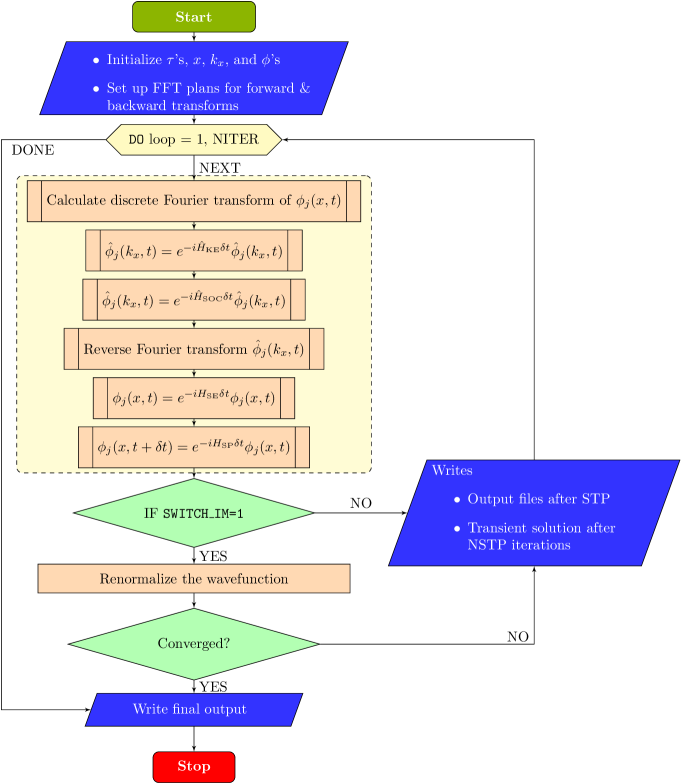
Figure 1: Flowchart illustrating the implementation of numerical procedure

Table 2: Description of various subroutines and functions involved in program and their usage.

Name	Type	Description
INITIALIZE	Subroutine	Defines the spatial and Fourier grids, trapping potential, and initializes the component wave functions
CREATE_PLANS	Subroutine	Creates FFTW plans (with threads) for forward and backward transforms
DESTROY_PLANS	Subroutine	Destroys FFTW plans for forward and backward transforms
FFT	Subroutine	Calculates the discrete forward Fourier transform
KE	Subroutine	Solves the split-equation corresponding to $H_{\rm KE}$ in Fourier space
SOC	Subroutine	Solves the split-equation corresponding to $H_{\rm SOC}$ in Fourier space
BFT	Subroutine	Calculates the discrete backward Fourier transform of component wavefunctions
SE	Subroutine	Solves the split-equation corresponding to $H_{\rm SE}$
SP	Subroutine	Solves the split-equation corresponding to $H_{\rm SP}$
FXYZ	Subroutine	Calculates $F_{x}$ (FX), $F_{y}$ (FY) and $F_{z}$ (FZ) to evaluate $F_{-}$ (FMINUS) and $F_{+}$ (FPLUS)
MAT_C	Subroutine	Calculates $H_{12}$ (C12), $H_{13}$ (C13), $H_{23}$ (C23), $H_{34}$ (C34), $H_{35}$ (C35) and $H_{45}$ (C45), i.e. the elements of $H_{SE}$.
NORMT	Subroutine	Normalizes the total density to 1
NEWTON	Subroutine	Solves the non-linear Eqs. (24a)-(24b) by using Newton Raphson method
NORMC	Subroutine	Calculates the norm of individual components
RAD	Subroutine	Calculates the root mean square (rms) sizes of the five components
ENERGY	Subroutine	Calculates the five component chemical potentials $\mu$ (MU), energy $E$ (EN), and magnetization $\cal M$ (MZ)
SIMPSON	Function	Performs integration by Simpson’s $1/3$ rule
DIFF	Function	Evaluates $df(x)/dx$ using nine point Richardson’s extrapolation formula

5.2 Functions & subroutines

All the subroutines and functions, used in the three codes, and their specific tasks are listed in Table 2. The user does not need to make any changes to these subroutines and functions. The overall organization of the various procedures for ’imagtime1D_spin2.f90’ is illustrated in the flowchart provided in Fig. 1. The subroutine symbols in the flowchart, i.e. a rectangle with double-struck vertical edges, from the top to bottom, respectively, represent the successive calls to subroutines FFT, KE, SOC, BFT, SE, and SP.

The description of the various output files written by the codes is provided in Table 3. Besides these output files, in realtime-propagation mode, user needs to provide an input file ’initial_sol.dat’ whose contents are in the same format as ’solution_file_im.dat’.

Table 3: Description of various output files and their contents. ’*’ denotes ’im’ or ’re’.

Name	Time propagation	Contents
file1_*.dat	imaginary/real	Various input parameters are written at the top of file. Total norm, energy, chemical potentials and $|\phi_{j}|$’s at the origin are written after each NSTP iterations.
file2_*.dat	imaginary/real	Time, energy and rms sizes for individual components after each STP iterations
file3_*.dat	imaginary/real	Time, norm of the individual components, sum of norms of individual components , and magnetization after each STP iterations
convergence.dat	imaginary	Number of iterations and convergence attained after each STP iterations.
tmp_solution_file.dat	imaginary/real	Component densities $\rho_{j}$ and their corresponding phases are written at every space point and updated after each NSTP iterations.
solution_file_*.dat	imaginary/real	Final component densities $\rho_{j}$ and their corresponding phases are written at every space point.

We have described here the 1D code, but the structure of code in 2D and 3D is identical. The names and role of modules, subroutines, and functions in three codes are also same. The main difference would be due to the fact that in 2D program, spatial grid consists of NX and NY points with spatial step sizes DX and DY along $x$ and $y$ directions, respectively. The resultant spatial domain along these directions would be LX = DX${\times}$NX and LY = DY${\times}$NY, respectively. Similarly, in 3D program, spatial grid consists of total of NX$\times$NY$\times$NZ points with spatial step sizes of DX, DY, and DZ along three directions.

6 OpenMP Parallelization

For the three codes, we have tested the performance of OpenMP parallelization for their imaginary as well as real-time variants on a 24-core Intel^® Xeon^® Platinum 8160 CPU@ 2.10 GHz processor. The OpenMP performances of the imaginary time and real-time variants are quite similar. The array sizes considered to perform these parallelization tests are NX = 50000, NX = NY = 1024, and NX = NY = NZ = 128 for 1D, 2D and 3D codes, respectively. We measured the elapsed wall clock time for 1000 iterations starting from the INITIALIZE subroutine and have not counted the time spent in opening/closing and reading/writing the data files. We have studied the performance of these codes with Intel Fortran 18.0.3 and GNU Fortran 5.4.0 compilers using upto 24 processors and confirmed that our OpenMP Fortran programs are optimized for both the compilers. A significant decrease in execution time has been observed for all the codes as is quite clear from the test results presented for the imaginary time variants in Fig. 2.

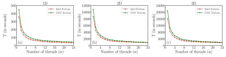
Figure 2: (Color online) (a) Execution time for 1000 iterations (in seconds) as a function of number of threads for 1D code compiled with GNU Fortran 5.4.0 and Intel Fortran 18.0.3 compilers for imaginary time propagation. (b) and (c) are the same for 2D and 3D codes.

To get the quantitative estimate of OpenMP parallelization, we have calculated the speedup and efficiency for all these codes for both the compilers, where speedup is defined as the ratio of execution time with 1 thread to the execution time with $n$ threads and efficiency is the ratio of speedup to the number of threads. We have achieved an excellent speedup of above 10 with 24 threads for 1D code and above 9 for 2D as well as 3D codes with aforementioned compilers as shown in Fig. 3. All these tests have been performed with non-zero value of SOC strength.

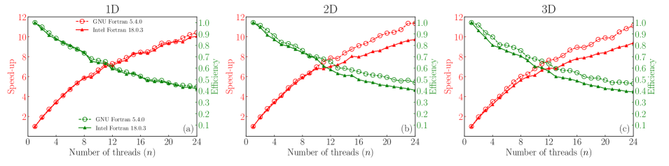
Figure 3: (Color online) Speedup and efficiency as a function of number of threads (n) are shown for imaginary time propagation. Figures (a)-(c) show the results for 1D, 2D and 3D codes, respectively.

7 Numerical Results

In this section, we present the numerical results for energies, chemical potentials, and densities of the ground states of q1D, q2D and 3D spin-2 BECs. We also present the results for dynamics of a q1D BEC.

7.1 Results for q1D systems

Here we present the results for q1D BECs first in the absence of SO coupling and then in the presence of SO coupling followed by the results for dynamics in the presence of SO coupling.

Without SO coupling, $\gamma_{x}$ = 0

We consider (a) ⁸³Rb, (b) ²³Na, and (c) ⁸⁷Rb spin-2 BECs as the typical examples of ferromagnetic, anti-ferromagnetic and cyclic phases. The three scattering length values considered for these systems are [2, 9]

$${\rm(a)}\quad a_{0} = 83.0a_{B},\quad a_{2}=82.0a_{B},\quad a_{4}=81.0a_{B};$$

$${\rm(b)}\quad a_{0} = 34.9a_{B},\quad a_{2}=45.8a_{B},\quad a_{4}=64.5a_{B};$$

$${\rm(c)}\quad a_{0} = 87.93a_{B},\quad a_{2}=91.28a_{B},\quad a_{4}=99.18a_{B},$$

respectively. We consider $10000$ atoms of each of these systems trapped in q1D trapping potential with $\omega_{x}=2\pi\times 20$Hz, $\omega_{y}=\omega_{z}=2\pi\times 400$Hz, and thus $\alpha_{x}=1$ and $\alpha_{y}=\alpha_{z}=20$. The oscillator lengths for the three systems are $2.47~{}\mu$m for (a), $4.69~{}\mu$m for (b), and $2.41~{}\mu$m for (c). The triplet of dimensionless interaction strengths $(\tau_{0},\tau_{1},\tau_{2})$ are given as

$${\rm(a)}\quad(\tau_{0},\tau_{1},\tau_{2}) = (699.62,-1.23,4.90),$$

$${\rm(b)}\quad(\tau_{0},\tau_{1},\tau_{2}) = (242.97,12.06,-13.03),$$

$${\rm(c)}\quad(\tau_{0},\tau_{1},\tau_{2}) = (831.26,9.91,0.31).$$

For the conversion of dimensional variables to their dimensionless analogues, we refer the reader to Ref. [19]. For ⁸³Rb the results obtained by solving Eqs. (1a)-(1c) are compared with SCSM, viz. Eqs. (6)-(9), with $g=\tau_{0}+4\tau_{1}$. Similarly, for ²³Na and ⁸⁷Rb spin-2 BECs, the results are compared with TCSM, viz. Eqs. (10a)-(11b) for the former and Eqs. (12a)-(12b) and Eq. (14) for the latter. The ground state chemical potentials and energies obtained for q1D ⁸³Rb using the full mean-field and scalar models are given in table 4 with various values of $\cal M$. Similarly, comparisons of chemical potentials and energies from both the models for q1D ²³Na and ⁸⁷Rb are presented in table 5 and 6, respectively. The agreement between the two set of results is excellent and is also evident from ground state density profiles for the three systems shown in Fig. 4.

Table 4: Ground state energies and chemical potential values of q1D ⁸³Rb BEC obtained with spin-2 mean-field model and SCSM. The results have been obtained with $\Delta x=0.05$ and $\Delta t=0.000125$ for different values of $\cal M$.

	Eqs. (1a)-(1c)	SCSM	83Rb
${\cal M}$	$\mu_{\pm 2}=\mu_{\pm 1}=\mu_{0}$	$\mu=\mu_{\pm 2}=\mu_{\pm 1}=\mu_{0}$	$E$	$E$ - SCSM
0-1.9	51.3976	51.3991	30.8496	30.8496

Table 5: Ground state energies and chemical potential values of q1D ²³Na BEC obtained with spin-2 mean-field model and TCSM. The results have been obtained with $\Delta x=0.05$ and $\Delta t=0.000125$ for different values of $\cal M$.

	Eqs. (1a)-(1c)		TCSM		23Na
${\cal M}$	$\mu_{+2}$	$\mu_{-2}$	$\mu_{+2}$	$\mu_{-2}$	$E$	$E$- TCSM
0.0	25.3397	25.3397	25.3397	25.3397	15.2216	15.2216
0.2	25.7025	24.9641	25.7025	24.9641	15.2401	15.2401
0.4	26.0570	24.5702	26.0570	24.5702	15.2956	15.2956
0.6	26.4064	24.1517	26.4064	24.1517	15.3891	15.3891
0.8	26.7530	23.7013	26.7530	23.7013	15.5216	15.5216
1.0	27.0978	23.2103	27.0978	23.2103	15.6949	15.6949
1.2	27.4410	22.6678	27.4410	22.6678	15.9112	15.9112
1.4	27.7824	22.0565	27.7824	22.0565	16.1733	16.1733
1.6	28.1220	21.3449	28.1220	21.3449	16.4854	16.4854
1.8	28.4597	20.4577	28.4597	20.4577	16.8538	16.8538

Table 6: Ground state energies and chemical potential values of q1D ⁸⁷Rb BEC obtained with the spin-2 mean-field model and the TCSM. The results have been obtained with $\Delta x=0.05$ and $\Delta t=0.000125$ for different values of $\cal M$.

	Eqs. (1a)-(1c)		TCSM		87Rb
${\cal M}$	$\mu_{+2}$	$\mu_{-1}$	$\mu_{+2}$	$\mu_{-1}$	$E$	$E$- TCSM
0.1	58.0251	57.8798	58.0251	57.8798	34.7691	34.7691
0.3	58.2121	57.7760	58.2121	57.7760	34.7884	34.7884
0.5	58.3952	57.6631	58.3952	57.6631	34.8273	34.8273
0.7	58.5766	57.5383	58.5766	57.5383	34.8863	34.8863
0.9	58.7578	57.3979	58.7578	57.3979	34.9661	34.9661
1.1	58.9393	57.2376	58.9393	57.2376	35.0680	35.0680
1.3	59.1209	57.0512	59.1209	57.0512	35.1936	35.1936
1.5	59.3026	56.8284	59.3026	56.8284	35.3448	35.3448
1.7	59.4841	56.5485	59.4841	56.5485	35.5247	35.5247
1.9	59.6655	56.1488	59.6655	56.1488	35.7387	35.7387

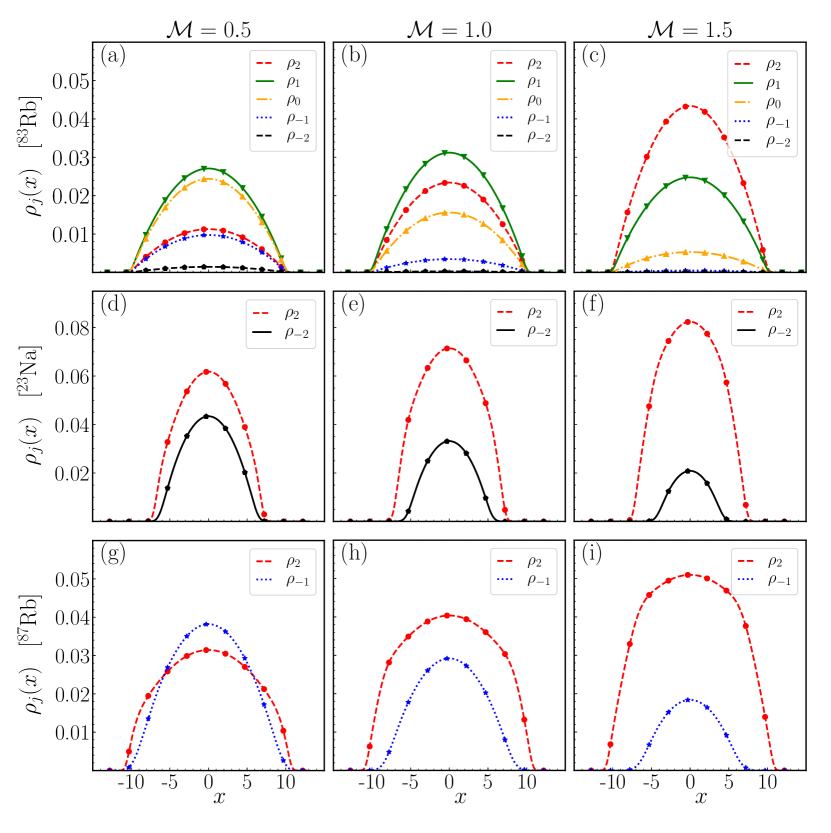
Figure 4: (Color online) (a)-(c) are numerically calculated ground state component densities with the full mean-field model (indicated by different line styles) and the scalar model (indicated by different point styles) for a spin-2 BEC of ⁸³Rb with different values of ${\cal M}$. (d)-(f) and (g)-(i) are the same for ²³Na and ⁸⁷Rb, respectively.

With SO coupling, $\gamma_{x}\neq 0$

In the presence of SO coupling, for ⁸³Rb, ²³Na and ⁸⁷Rb, we again consider the same parameters as we have chosen for $\gamma_{x}=0$ in Sec. 7.1. The values of individual component chemical potentials and total energies for ⁸³Rb, ²³Na, ⁸⁷Rb with various values of $\gamma_{x}$ are presented in tables 7, 8 and 9, respectively. The component densities for three systems with $\gamma_{x}=0.25$, 0.5 and 0.7 are illustrated in Fig. 5.

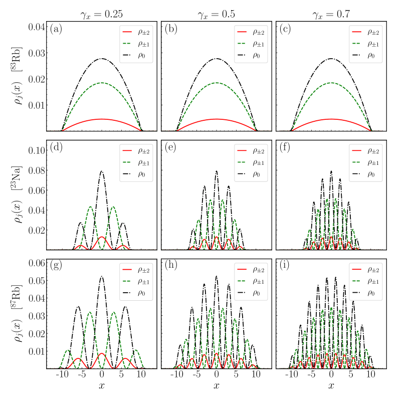
Figure 5: (Color online) (a)-(c) Numerically calculated ground state densities for an SO-coupled ⁸³Rb with $\gamma_{x}=0.25,0.5,$ and $0.7$, respectively. The same for ²³Na and ⁸⁷Rb are shown in sub-figures (d)-(f) and (g)-(i), respectively.

Table 7: Ground state energies and chemical potential values of ⁸³Rb condensates in the presence of SO coupling with $\Delta x=0.05$ , $\Delta t=0.000125$

.

$\gamma_{x}$	$\mu_{2}$	$\mu_{1}$	$\mu_{0}$	$\mu_{-1}$	$\mu_{-2}$	Energy
0.1	51.3774	51.3774	51.3774	51.3774	51.3774	30.8296
0.2	51.3172	51.3172	51.3172	51.3172	51.3172	30.7696
0.3	51.2169	51.2169	51.2169	51.2169	51.2169	30.6696
0.4	51.0764	51.0764	51.0764	51.0764	51.0764	30.5296
0.5	50.8958	50.8958	50.8958	50.8958	50.8958	30.3496
0.6	50.6751	50.6751	50.6751	50.6751	50.6751	30.1296
0.7	50.4142	50.4142	50.4142	50.4142	50.4142	29.8696
0.8	50.1131	50.1131	50.1131	50.1131	50.1131	29.5696
0.9	49.7720	49.7720	49.7720	49.7720	49.7720	29.2296
1.0	49.3907	49.3907	49.3907	49.3907	49.3907	28.8496

Table 8: Ground state energies and chemical potential values of ²³Na condensates in the presence of SO coupling with $\Delta x=0.05$ , $\Delta t=0.000125$

.

$\gamma_{x}$	$\mu_{2}$	$\mu_{1}$	$\mu_{0}$	$\mu_{-1}$	$\mu_{-2}$	Energy
0.1	25.3192	25.3199	25.3192	25.3199	25.3192	15.2016
0.2	25.2588	25.2597	25.2588	25.2597	25.2588	15.1416
0.3	25.1591	25.1593	25.1591	25.1593	25.1591	15.0416
0.4	25.0186	25.0193	25.0186	25.0193	25.0186	14.9016
0.5	24.8385	24.8388	24.8385	24.8388	24.8385	14.7216
0.6	24.6181	24.6185	24.6181	24.6185	24.6181	14.5016
0.7	24.3576	24.3581	24.3576	24.3581	24.3576	14.2416
0.8	24.0572	24.0575	24.0572	24.0575	24.0572	13.9416
0.9	23.7165	23.7170	23.7165	23.7170	23.7165	13.6016
1.0	23.3360	23.3363	23.3360	23.3363	23.3360	13.2216

Table 9: Ground state energies and chemical potential values of ⁸⁷Rb condensates in the presence of SO coupling with $\Delta x=0.05$ , $\Delta t=0.000125$

.

$\gamma_{x}$	$\mu_{2}$	$\mu_{1}$	$\mu_{0}$	$\mu_{-1}$	$\mu_{-2}$	Energy
0.1	57.9121	57.9121	57.9120	57.9121	57.9121	34.7484
0.2	57.8518	57.8516	57.8518	57.8516	57.8518	34.6884
0.3	57.7513	57.7513	57.7513	57.7513	57.7513	34.5884
0.4	57.6108	57.6108	57.6108	57.6108	57.6108	34.4484
0.5	57.4302	57.4300	57.3402	57.4300	57.4302	34.2684
0.6	57.2092	57.2093	57.2092	57.2093	57.2092	34.0484
0.7	56.9483	56.9482	56.9483	56.9482	56.9483	33.7884
0.8	56.6471	56.6470	56.6471	56.6470	56.6471	33.4884
0.9	56.3058	56.3058	56.3058	56.3058	56.4058	33.1484
1.0	55.9243	55.9243	55.9243	55.9243	55.9243	32.7684

7.1.1 Real-time Dynamics

We consider q1D ⁸³Rb BEC with SO coupling strength $\gamma_{x}=0.5$ to illustrate an example of the real-time dynamics which can be investigated with the three programs. We prepare an initial solution with a fixed magnetization of $0.5$ using imaginary-time propagation. Fixing the magnetization ensures that the solution obtained with imaginary-time propagation is not the ground state; as to obtain the ground state solution, shown in Fig. 5(b), magnetization is not fixed in imaginary-time propagation. Hence the solution is expected to show spin-mixing dynamics when evolved in real time. This is evident from variation of the component norms $N_{j}$’s and magnetization ${\cal M}$ as a function of time $t$ shown in Figs. 6(a) and 6(b), respectively.

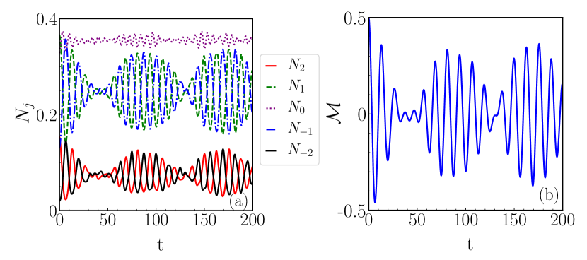
Figure 6: (Color online) (a) Component norms and (b) magnetization as a function of time for ⁸³Rb with $\tau_{0}=699.62$, $\tau_{1}=-1.23$, and $\tau_{2}=4.90$ with magnetization at $t=0$ set to $0.5$.

7.2 Results for q2D spin-2 BECs

Here also, we consider three cases (a) ⁸³Rb, (b) ²³Na, and (c) ⁸⁷Rb spin-2 BECs. We consider $10000$ atoms of these systems trapped in q2D trapping potential with $\omega_{x}=\omega_{y}=2\pi\times 20$ Hz, $\omega_{z}=2\pi\times 400$ Hz, and thus $\alpha_{x}=\alpha_{y}=1$ and $\alpha_{z}=20$. The triplet of dimensionless interaction strengths $(\tau_{0},\tau_{1},\tau_{2})$ for these cases are given as

$${\rm(a)}\quad(\tau_{0},\tau_{1},\tau_{2}) = (392.14,-0.67,2.74),$$

$${\rm(b)}\quad(\tau_{0},\tau_{1},\tau_{2}) = (136.18,6.76,-7.30),$$

$${\rm(c)}\quad(\tau_{0},\tau_{1},\tau_{2}) = (465.92,5.55,0.18).$$

The comparison of ground state energies between full mean-field model and scalar models of spin-2 BEC for all three cases with different values of magnetization is excellent as is reported in Table 10.

In the presence of SO coupling, we also illustrate some of the qualitatively distinct numerically obtained ground state solutions for q2D configurations. We consider interaction parameters’ set (a) with $\gamma_{x}=1$ and $\gamma_{y}=0.25$, set (b) with $\gamma_{x}=\gamma_{y}=0.5$, and set (c) with $\gamma_{x}=0.1$ and $\gamma_{y}=0.5$. The distinct nature of density profiles for the three cases is evident from Figs. 7(a)-(o). The ground state solution for ⁸³Rb is a plane-wave solution with Gaussian density profiles for all the five components as is shown in Fig 7(a)-7(e). For ²³Na, ground state solution has vortices of winding numbers $-2,-1,0,+1,$ and $+2$ associated with $m_{f}=+2,+1,0,-1,$ and $-2$ components, respectively. The non-zero vorticity associated with components $m_{f}=\pm 1,\pm 2$ leads to the zero densities at the center of these components as is shown in Figs. 7(f)-(j). For ⁸⁷Rb, the ground state has horizontal stripe pattern in the component densities as is shown in Figs. 7(k)-(o).

We have also confirmed the accuracy of our codes by comparing our results with results reported in Ref. [11]. As per the parameters considered in Ref. [11], we consider q2D spin-2 BEC firstly with $\tau_{0}=2000,\tau_{1}=400$, $\tau_{2}=-400$, $\gamma_{x}=3$, $\gamma_{y}=1.5$ and secondly with $\tau_{0}=2000,\tau_{1}=40$, $\tau_{2}=400$, $\gamma_{x}=\gamma_{y}=2$. The ground state density profiles in these two cases as shown in Figs. 8(a)-(e) and Figs. 8(f)-(j), respectively, are in agreement with Ref. [11]. For all these 2D results reported in this subsection, we have considered spatial step sizes $\Delta$x = $\Delta$y = 0.05 and temporal step size $\Delta$t = 0.000125.

Table 10: Ground state energies of ⁸³Rb, ²³Na, and ⁸⁷Rb q2D spin-2 BECs obtained with full mean-field model and scalar models (SCSM for ⁸³Rb and TCSM for ²³Na and ⁸⁷Rb). The results have been obtained with $\Delta x=0.05$ and $\Delta t=0.000125$ for different values of $\cal M$.

	83Rb		23Na		87Rb
${\cal M}$	$E$	$E$ - SCSM	$E$	$E$- TCSM	$E$	$E$ - TCSM
0.0	7.5336	7.5336	4.5314	4.5314	8.2229	8.2229
0.2	7.5336	7.5336	4.5352	4.5352	8.2247	8.2247
0.4	7.5336	7.5336	4.5468	4.5468	8.2300	8.2300
0.6	7.5336	7.5336	4.5662	4.5662	8.2388	8.2388
0.8	7.5336	7.5336	4.5937	4.5937	8.2512	8.2512
1.0	7.5336	7.5336	4.6294	4.6294	8.2673	8.2673
1.2	7.5336	7.5336	4.6739	4.6739	8.2872	8.2872
1.4	7.5336	7.5336	4.7278	4.7278	8.3112	8.3112
1.6	7.5336	7.5336	4.7921	4.7921	8.3396	8.3396
1.8	7.5336	7.5336	4.8684	4.8684	8.3729	8.3729

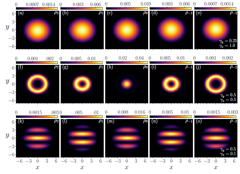
Figure 7: (Color online) (a)-(e) are the ground state component densities for an SO-coupled q2D spin-2 BEC with $\tau_{0}=392.14,\tau_{1}=-0.69,\tau_{2}=2.75$, $\gamma_{x}=1,$ and $\gamma_{y}=0.25$. (f)-(j) and (k)-(o) are the same for the SO-coupled spin-2 BECs with $\tau_{0}=136.18,\tau_{1}=6.76,\tau_{2}=-7.36$, $\gamma_{x}=0.5,\gamma_{y}=0.5$ and $\tau_{0}=465.920,\tau_{1}=5.55,\tau_{2}=0.18,\gamma_{x}=0.1,\gamma_{y}=0.5$, respectively.

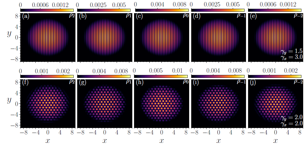
Figure 8: (Color online) (a)-(e) are the ground state component densities for an SO-coupled q2D spin-2 BEC with $\tau_{0}=2000,\tau_{1}=400,\tau_{2}=-400$, $\gamma_{x}=3$ and $\gamma_{y}=1.5$. (f)-(j) are the same for a spin-2 BEC with $\tau_{0}=2000,\tau_{1}=40,\tau_{2}=400$, $\gamma_{x}=\gamma_{y}=2$. These results are in agreement with Ref. [11]

7.3 Results for 3D spin-2 BECs

We consider a ²³Na spin-2 BEC with $\tau_{0}=76.33,\tau_{1}=3.79$, $\tau_{2}=-4.09$, $\alpha_{x}=\alpha_{y}=\alpha_{z}=1$ and spin-orbit coupling strengths $\gamma_{x}=\gamma_{y}=\gamma_{z}=0.5$. This set of parameters corresponds to 10000 ²³Na atoms trapped in an isotropic trapping potential with $\omega_{x}=\omega_{y}=\omega_{z}=2\pi\times 20$Hz. Here we obtain (-2,-1,0,+1,+2) type of vortex solution and corresponding energy is 1.9693. The 3D iso-surfaces corresponding to iso-density value of of $0.0007$ are shown in Fig. 9.

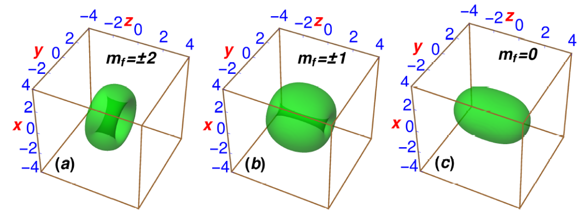
Figure 9: (a)-(c) 3D isosurfaces of component densities for an SO-coupled ²³Na spin-2 BEC with $\tau_{0}=76.33,\tau_{1}=3.79,\tau_{2}=-4.09$ and $\gamma_{x}=\gamma_{y}=\gamma_{z}=0.5$. The isosurfaces correspond to isodensity value of $0.0007$. The solution has been obtained with $\Delta x=0.1$ and $\Delta t=0.0005$.

8 Summary

We have provided a set of three OpenMP parallelized FORTRAN 90/95 programs to solve the CGPEs describing an $f=2$ spinor BEC with an anisotropic spin-orbit coupling in q1D, q2D and 3D configurations using the time-splitting Fourier spectral method. These codes can be used to simulate both static and dynamic properties of an SO-coupled spin-2 BEC with a variety of SO couplings including Rashba, Dresselhaus or a combination of both. We have confirmed the accuracy of the codes by comparing the the results for ground-state energies, chemical potentials and densities obtained from the codes with those available in the literature or with the simplified scalar models which show an excellent agreement. The test results for OpenMP performance parameters like speedup and efficiency are very good. With the advent of SO coupling in the spinor BECs, the present set of codes can be very useful to the researchers working on spin-2 BECs.

Appendix

Conservation/Non-conservation of Magnetization

In the absence of spin-orbit coupling, $\Gamma_{\pm 2}({\bf x},t)=0,\Gamma_{\pm 1}({\bf x},t)=0,\Gamma_{0}({\bf x},t)=0$,

$$\frac{d{\cal M}}{dt} = \int\left(2|\phi_{+2}({\bf x},t)|^{2}+|\phi_{+1}({\bf x},t)|^{2}-|\phi_{-1}({\bf x},t)|^{2}-2|\phi_{-2}({\bf x},t)|^{2}\right)d{\bf x},$$ (20)

$$= \int\left(2\frac{\partial\phi_{+2}}{\partial t}\phi_{+2}^{*}+2\phi_{+2}\frac{\partial\phi_{+2}^{*}}{\partial t}+\frac{\partial\phi_{+1}}{\partial t}\phi_{+1}^{*}+\phi_{+1}\frac{\partial\phi_{+1}^{*}}{\partial t}-\frac{\partial\phi_{-1}}{\partial t}\phi_{-1}^{*}\right.$$

$$\left.-\phi_{-1}\frac{\partial\phi_{-1}^{*}}{\partial t}-2\frac{\partial\phi_{-2}}{\partial t}\phi_{-2}^{*}-2\phi_{-2}\frac{\partial\phi_{-2}^{*}}{\partial t}\right)d{\bf x}.$$

Using Eqs. (1a)-(1c) in Eq. (20), we obtain

$$\frac{d{\cal M}}{dt} = -i\tau_{1}\int\left(F_{-}\phi_{+1}\phi_{+2}^{*}-F_{+}\phi_{+1}^{*}\phi_{+2}-F_{+}\phi_{-1}\phi_{-2}^{*}+F_{-}\phi_{-1}^{*}\phi_{-2}+\sqrt{\frac{3}{2}}F_{-}\phi_{0}\phi_{+1}^{*}\right.$$ (21)

$$\left.-\sqrt{\frac{3}{2}}F_{+}\phi_{0}^{*}\phi_{+1}-\sqrt{\frac{3}{2}}F_{+}\phi_{0}\phi_{-1}^{*}+\sqrt{\frac{3}{2}}F_{-}\phi_{0}^{*}\phi_{-1}\right)d{\bf x},$$

$$= -i\tau_{1}\int\left[F_{-}\left(\phi_{+1}\phi_{+2}^{*}+\phi_{-1}^{*}\phi_{-2}+\sqrt{\frac{3}{2}}\phi_{0}^{*}\phi_{-1}+\sqrt{\frac{3}{2}}\phi_{0}\phi_{+1}^{*}\right)\right.$$

$$\left.-F_{+}\left(\phi_{+1}^{*}\phi_{+2}+\phi_{-1}\phi_{-2}^{*}+\sqrt{\frac{3}{2}}\phi_{0}^{*}\phi_{+1}+\sqrt{\frac{3}{2}}\phi_{0}\phi_{-1}^{*}\right)\right]d{\bf x},$$

$$= -i\tau_{1}\int\left(F_{-}\frac{F_{+}}{2}-F_{+}\frac{F_{-}}{2}\right)d{\bf x}$$

$$= 0.$$

In the presence of SO coupling, combining Eqs. (1a)-(1c) with Eq. (20) leads to

$$\frac{d{\cal M}}{dt} = -i\int\left(2\phi_{+2}^{*}\Gamma_{+2}+2\phi_{+2}\Gamma_{+2}^{*}+\phi_{+1}^{*}\Gamma_{+1}+\phi_{+1}\Gamma_{+1}^{*}-2\phi_{-2}^{*}\Gamma_{-2}+2\phi_{-2}\Gamma_{-2}^{*}\right.$$ (22)

$$\left.+\phi_{-1}^{*}\Gamma_{-1}+\phi_{-1}\Gamma_{-1}^{*}\right)d{\bf x}$$

$$\neq 0,$$

in general. Therefor ${\cal M}$ is conserved in the absence of SO coupling, but not so, in general, in the presence of SO coupling.

Simultaneous conservation of Norm and Magnetization

We use imaginary time propagation method, where $t$ is replaced by $-i\tau$ in CGPEs, viz. Eqs. (1a)-(1c), to determine the stationary states of the system. Now, as the imaginary time propagation used to calculate the ground state of the system under the constraint of fixed norm and magnetization, conserves neither of the two, one needs to renormalize the component wavefunctions after each time iteration. This means after each imaginary-time step $\delta\tau$, the component wavefunctions are rescaled as $\phi_{j}({\bf x},\tau+\delta t)=\sigma_{j}\phi_{j}({\bf x},\tau),$ where $\sigma_{j}$’s are renormalization factors. These renormalization factors $\sigma_{j}$’s satisfy the following relationships among them [21]

$$\sigma_{1}\sigma_{-1}=\sigma_{0}^{2},$$ (23a)

$$\sigma_{2}\sigma_{-2}=\sigma_{0}^{2},$$ (23b)

$$\sigma_{2}\sigma_{-1}^{2}=\sigma_{0}^{3},$$ (23c)

and

$$u^{4}N_{2}+u^{3}vN_{1}+u^{2}v^{2}N_{0}+uv^{3}N_{-1}+v^{4}N_{-2}={\cal N},$$ (24a)

$$2u^{4}N_{2}+u^{3}vN_{1}-uv^{3}N_{-1}-2v^{4}N_{-2}={\cal M}$$ (24b)

with norm and magnetization, where $u=\sigma_{1}^{2}$ and $v=\sigma_{0}^{2}$ and $N_{j}=\int|\phi_{j}({\bf x},\tau)|^{2}d{\bf x}$ are the component norms at (imaginary) time $\tau$. In the present work, we solve Eqs. (24a)-(24b) using Newton-Raphson method after each iteration in imaginary time. The $\sigma_{1}$ and $\sigma_{0}$ so obtained can be substituted back in Eqs. (23a)-(23c) to determine the remaining renormalization factors $\sigma$’s. The simultaneous fixing of norm and magnetization is only implemented in the absence of SO coupling.

References

- [1] D.M. Stamper-Kurn, M.R. Andrews, A.P. Chikkatur, S. Inouye, H.-J. Miesner, J. Stenger, and W. Ketterle, Phys. Rev. Lett. 80 (1998) 2027.
- [2] C.V. Ciobanu, S.-K. Yip, and T.-L. Ho Phys. Rev. A 61 (2000) 033607.
- [3] M. Ueda and M. Koashi, Phys. Rev. A 65 (2002) 063602.
- [4] M.-S. Chang, C.D. Hamley, M.D. Barrett, J.A. Sauer, K.M. Fortier, W. Zhang, L. You, and M.S. Chapman, Phys. Rev. Lett. 92 (2004) 140403
- [5] H. Schmaljohann, M.Erhard, J. Kronjäger, M. Kottke, S. Van Staa, L. Cacciapuoti, JJ. Arlt, K. Bongs and K. Sengstock, Phys. Rev. Lett. 92 (2004) 040402.
- [6] T.Kuwamoto, K. Araki and T.Hirano, Phys. Rev. A. 69 (2004) 063604.
- [7] A. Widera, F. Gerbier, S. Fölling, T. Gericke, O. Mandel, and I. Bloch, Phys. Rev. Lett. 95 (2005) 190405.
- [8] Y. Kawaguchi and M. Ueda Phys. Rev. A 84, (2011) 053616.
- [9] A. Widera, F. Gerbier, S. Fölling, T. Gericke, O. Mandel and I. Bloch, New Journal of Physics 8 (2006) 152.
- [10] Y.-J. Lin, K. Jiménez-García, and I.B. Spielman, Nature 471 (2011) 83; D.L. Campbell, R.M. Price, A. Putra, A. Valdés-Curiel, D. Trypogeorgos, and I.B. Spielman, Nature Communications 7 (2016) 10897; X. Luo, L. Wu, J. Chen, Q. Guan, K. Gao, Zhi-Fang Xu, L. You, and R. Wang, Scientific Reports 6 (2016) 18983.
- [11] Z.F. Xu, R. L, and L. You Phys. Rev. A 83 (2011) 053602.
- [12] T. Kawakami, T. Mizushima, and K. Machida Phys. Rev. A 84 (2011) 011607(R); Z. F. Xu, Y. Kawaguchi, L. You, and M. Ueda, Phys. Rev. A 86 (2012) 033628.
- [13] B. M. Anderson,I. B. Spielman, and G. Juzeliūnas, Phys. Rev. Lett. 111 (2013) 125301; Z.-F. Xu, L. You, and M. Ueda, Phys. Rev. Rev. A 87 (2013) 063634.
- [14] Y. Kawaguchi, M. Ueda, Physics Reports 520 (2012) 253-381.
- [15] H. Wang, Int. J. Comp. Math. 84 (2007) 925; W. Bao and F.Y. Lim., SIAM Journal on Scientific Computing 30 (2008) 1925; W. Bao, I.-L. Chern, and Y. Zhang, J. Comp. Phys. 253 (2013) 189.
- [16] H. Wang, J. Comp. Phys. 230 (2011) 6165.
- [17] H. Wang, J. Comp. Phys. 274 (2014) 473.
- [18] H. Wang and Z. Xu, Comp. Phys. Comm. 185 (2014) 2803.
- [19] P. Kaur, A. Roy, and S. Gautam, Comp. Phys. Comm. 259 (2021) 107671.
- [20] Y.A. Bychkov and E.I. Rashba, J. Phys. C: Solid state physics 17 (1984) 6039.
- [21] S. Gautam and S. K. Adhikari, Phys. Rev. A 91 (2015) 013624.
- [22] S. Gautam and S. K. Adhikari, Phys. Rev. A 92 (2015) 023616.
- [23] L.E. Young-S., P. Muruganandam, S.K. Adhikari, V. Loncar, D. Vudragovic, A. Balaz Comput. Phys. Commun. 220 (2017) 503; V. Loncar, L.E. Young-S., S. Skrbic, P. Muruganandam, S.K. Adhikari, Antun Balaz Comput. Phys. Commun. 209 (2016) 190; L.E. Young-S., D. Vudragovic, P. Muruganandam, S.K. Adhikari, A. Balaz Comput. Phys. Commun. 204 (2016) 209; B. Sataric, V. Slavnic, A. Belic, A. Balaz, P. Muruganandam, S.K. Adhikari Comput. Phys. Commun. 200 (2016) 411; V. Loncar, A. Balaz, A. Bogojevic, S. Skrbic, P. Muruganandam, S.K. Adhikari Comput. Phys. Commun. 200 (2016) 406; D. Vudragovic, I. Vidanovic, A. Balaz, P. Muruganandam, S.K. Adhikari Comput. Phys. Commun. 183 (2012) 2021; X. Antoine and R. Duboscq Comput. Phys. Commun. 185 (2014) 2969; X. Antoine and R. Duboscq Comput. Phys. Commun. 193 (2015) 95; Ž. Marojević and E. Göklü and Claus Lämmerzahl Comput. Phys. Commun. 202 (2016) 216
- [24] S.-M. Chang, W.-W. Lin, and S.-F. Shieh, J. Comp. Phys. 202 (2005) 367; W. Bao and J. Shen, SIAM Journal on Scientific Computing 26 (2005) 2010.
- [25] R. Ravisankar, D. Vudragović, P. Muruganandam, A. Balaž, S.K.Adhikari, Comp. Phys. Comm. 259 (2021) 107657.
- [26] http://www.fftw.org/