GASP XXXII. Measuring the diffuse ionized gas fraction in ram-pressure stripped galaxies

Abstract

The diffuse ionized gas (DIG) is an important component of the interstellar medium and it can be affected by many physical processes in galaxies. Measuring its distribution and contribution in emission allows us to properly study both its ionization and star formation in galaxies. Here, we measure for the first time the DIG emission in 38 gas-stripped galaxies in local clusters drawn from the GAs Stripping Phenomena in galaxies with MUSE survey (GASP). These galaxies are at different stages of stripping. We also compare the DIG properties to those of 33 normal galaxies from the same survey. To estimate the DIG fraction (C_DIG) and derive its maps, we combine attenuation corrected H$\alpha$ surface brightness with $\rm[S\textsc{II}]/H\alpha$ line ratio. Our results indicate that we cannot use neither a single H$\alpha$ or $\rm[S\textsc{II}]/H\alpha$ value, nor a threshold in equivalent width of H$\alpha$ emission line to separate spaxels dominated by DIG and non-DIG emission. Assuming a constant surface brightness of the DIG across galaxies underestimates C_DIG. Contrasting stripped and non-stripped galaxies, we find no clear differences in C_DIG. The DIG emission contributes between 20% and 90% of the total integrated flux, and does not correlate with the galactic stellar mass and star-formation rate (SFR). The C_DIG anti-correlates with the specific SFR, which may indicate an older ($>10^{8}$ yr) stellar population as ionizing source of the DIG. The DIG fraction shows anti-correlations with the SFR surface density, which could be used for a robust estimation of integrated C_DIG in galaxies.

1 Introduction

The interstellar medium (ISM) is an important component of galaxies that determines the galactic evolution and morphology through star formation (SF), regulates the exchange of chemical elements within galaxies, and affects many physical processes that leave observable signatures in the emitted and absorbed light (Schmidt 1959, Kennicutt 1998a, Kennicutt 1998b, Draine 2011, Calzetti et al. 1994). Physical processes outside and within galaxies, such as interactions, gas stripping, stellar and active galactic nucleus (AGN) feedback, and gravity, also affect the properties and distribution of various ISM components. Therefore, observations of the ISM at different wavelengths allows us to trace its different components and track the interplay of different physical mechanisms in galaxies.

The diffuse ionized gas (DIG), also known as Warm Ionized Medium (WIM) in the Milky Way, is one of the main components of the ISM (Reynolds 1984, Reynolds & Cox 1992, Walterbos & Braun 1994, Madsen et al. 2006, Haffner et al. 2009, Rueff et al. 2013, Barnes et al. 2014, Vale Asari & Stasińska 2020). It is an extended ionized gas between star forming regions (H II), reaching scale-heights of up to 1-2 kpc in the vertical line of sight from galactic disks, further than a typical size ($\approx 50$ pc) of star-forming associations (Reynolds & Cox 1992, Haffner et al. 2009, Bocchio et al. 2016, Tomičić et al. 2017). Furthermore, the DIG is warmer (temperatures higher than $\sim 10^{4}$ K) and less dense ($\rho\sim 10^{-1}$ cm^-3) than the gas in the H II regions (Collins & Rand 2001, Reynolds et al. 2001, Haffner et al. 2009, Barnes et al. 2014 Della Bruna et al. 2020). The DIG emission has lower surface brightness of the Balmer lines compared to the H II regions and associations (Reynolds 1984, Reynolds & Cox 1992, Kreckel et al. 2016, Kumari et al. 2019). It also shows higher values of [SII]/H$\alpha$ emission line ratios ($\rm[S\textsc{II}]\,\lambda 6717,6731/H\alpha>0.2$) compared to the ionized gas in typical H II regions ($\rm[S\textsc{II}]\,\lambda 6717,6731/H\alpha\approx 0.1$), likely due to higher temperatures and lower densities (Reynolds 1984, Madsen et al. 2006, Blanc et al. 2009, Kreckel et al. 2013).

The ionizing source of the DIG is not yet conclusively determined, although multiple sources may contribute. The dominant source may be leaked radiation from the OB stars, whose ionizing photons are able to escape dusty regions surrounding H II regions, thus ionizing gas at larger galactic scale-heights (Reynolds & Cox 1992, Minter & Balser 1998, Haffner et al. 2009). The relatively few ionizing photons coming from a large amount of hot, old and low-mass evolved stars (HOLMES) could explain large amounts of the DIG across galaxies (Flores-Fajardo et al. 2011a, Lacerda et al. 2018). Other ionizing sources are required to reproduce certain line rations observed in the DIG (Otte et al. 2002, Hoopes & Walterbos 2003). For example, the DIG may be heated and ionized by supernova shocks and turbulence (Slavin et al. 1993, Minter & Spangler 1997) or/and magnetic reconnection (Raymond 1992). According to Weingartner & Draine (2001), the electrons from heated dust at larger scale-heights may contribute in ionizing the gas, while Barnes et al. (2014) invoked ionization due to cosmic rays. Lastly, Slavin et al. (1993) and Binette et al. (2009) found in their models that the turbulent mixing of the layers of hot and cold gas could explain the observed line ratios, and higher temperatures.

In the literature, the detection and measurements of the DIG fraction (i.e. the fraction of the gas emission from the DIG to the total gas) is typically done based on one of the following methods: 1) using a threshold in H$\alpha$ surface brightness (using unresolved samples of galaxies or spatially resolved images), 2) using a threshold in [SII]/H$\alpha$ ratio, 3) using the criterion that H$\alpha$ equivalent width is $\rm W_{H\alpha}<3$ Å  or 4) combining and fitting the relation between the H$\alpha$ surface brightness and $\rm[S\textsc{II}]/H\alpha$ ratio, (Oey et al. 2007, Blanc et al. 2009, Kaplan et al. 2016, Lacerda et al. 2018, Kreckel et al. 2016, Zhang et al. 2017, Poetrodjojo et al. 2019, den Brok et al. 2020). Note that the last method assumes the same gas-phase metallicity throughout the galaxy. This assumption is good enough when a small part of the galaxy is probed, but it might not hold when larger portions of galaxies are investigated. In this case, metallicity variations within the galaxy, which affect the [SII]/H$\alpha$ ratio (Blanc et al. 2015), should be taken into account.

Observations show that the DIG emission in galaxies accounts for between 20% and 80% of the H$\alpha$ emission and covers a large fraction of the galactic area (Hoopes et al. 1999, Oey et al. 2007, Sanders et al. 2017, Kreckel et al. 2016, Della Bruna et al. 2020). The importance of measuring the DIG distribution and brightness in galaxies lays in the fact that it may hinder measurements of various physical properties of galaxies. For example, since the DIG’s source of ionization may not come from the star-forming regions, values of star-formation rates (SFRs) may be overestimated if the DIG contribution, coming from sources other than star formation, is not removed. Furthermore, different relative distributions of dust, young stars and extended ionized gas may lead to a miscalculation of the attenuation values (A_V) of star-forming regions (Calzetti et al. 1994, Tomičić et al. 2017, Tomičić et al. 2019).

The observations of the DIG allow us to trace the physical processes affecting galaxies and their ISM, study stellar feedback affecting the surrounding ISM (Barnes et al. 2014, Vandenbroucke & Wood 2019), and the effects of collision and turbulent mixing of gas layers with different properties (Slavin et al. 1993, Binette et al. 2009, Fumagalli et al. 2014, Poggianti et al. 2019a). An interesting population of galaxies that might have their DIG affected by the environment includes galaxies that enter galaxy clusters, passing through a intracluster medium. Their gas is being stripped from the disk, due to the ram-pressure (RP). This stripped gas, also seen as ionized gas tails outside the galaxy disks, collapses and forms new stars. Observations of this kind of hydrodynamical interaction offer an opportunity to probe the physics of the ISM in different environments and study how it affects galaxy evolution. This includes investigating the DIG distribution, estimating the fraction of the surface brightness coming from the DIG, and the sources of ionization of the DIG.

The GASP project (GAs Stripping Phenomena in galaxies with MUSE; Poggianti et al. 2017a) has optical spectral observations of 114 galaxies, of which some are at different levels of the ram-pressure stripping process. Poggianti et al. (2019a) found that approximately 50% of the $\rm H\alpha$ emission in the debris tails of a subsample of GASP galaxies is diffuse, i.e. is not related to identifiable star-forming clumps. In their work, the star-forming clumps were determined based on the Balmer $\rm H\alpha$ line images (Poggianti et al. 2017a). These star-forming knots were used for evaluation of various properties of the galaxies and the H II regions, such as SFRs, gas-phase metallicity variations, source of ionisation etc. (George et al. 2018, Vulcani et al. 2019a, Poggianti et al. 2019b, Vulcani et al. 2020).

The purpose of this paper is to measure the distribution and fraction of the DIG across the GASP galaxies. This paper follows a number of papers investigating statistical properties of the GASP sample (e.g. Jaffé et al. 2018, Vulcani et al. 2018, Poggianti et al. 2019b, Poggianti et al. 2017b, Vulcani et al. 2019a, Franchetto et al. 2020, Gullieuszik et al. 2020, Vulcani et al. 2020). We present for the first time a comparison of the DIG fractions between galaxies that are being stripped and those which are not. The method that we use for estimating the DIG fraction combines both the H$\alpha$ surface brightness and the [SII]/H$\alpha$ ratio, also taking into account the metallicity variation within galaxies. We compare our results for the DIG fraction with the fractions derived based on the method using only the H$\alpha$ surface brightness, and look at how the [SII]/H$\alpha$ line ratio and equivalent width of H$\alpha$ line vary with the DIG fractions.

This paper is structured as follows. We describe the GASP project and the galaxy sample in Sec. 2. In the same section, we explain observations, data reduction and spectral analysis. Furthermore, we explain how we derived the emission line maps, gas-phase metallicities and equivalent width. In Sec. 3, we explain the method for estimating the fraction of the DIG. The results are presented in Sec. 4, and the implications of using various methods for estimating the DIG fraction are discussed in Sec. 5. Here, we will also show a comparison of the DIG fractions between the stripped and non-stripped galaxies. The conclusions and summary are written in Sec. 6.

In this paper we adopted standard cosmological constants of H${}_{0}=70$ km$\rm\,s^{-1}Mpc^{-1}$, $\rm\Omega_{M}=0.3$, $\Omega_{\Lambda}=0.7$, and the initial mass function (IMF) from Chabrier (2003).

2 Data

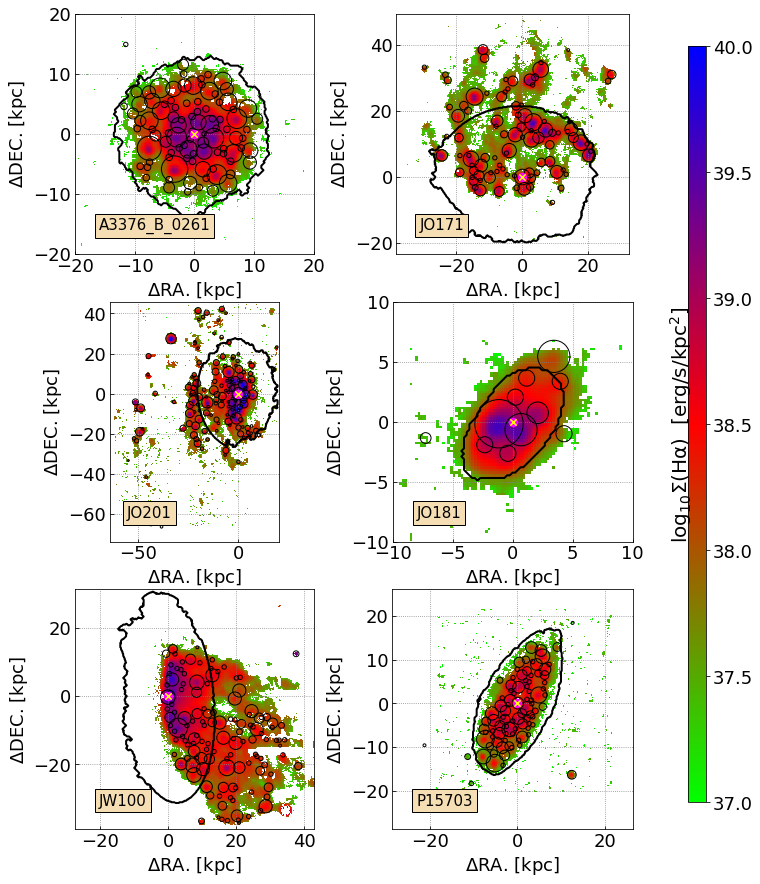
Figure 1: Maps of the observed surface brightness of H$\alpha$ emission ($\Sigma H\alpha$) of some galaxies in the GASP survey. The following galaxies are examples of a control sample galaxy ($\rm A3376\_B\_0261$), gas stripped galaxies (ring galaxy JO171, face-on JO201, low gas-phase metallicity JO181, and JW100), and a field galaxy (P15703). In each frame, we indicate the stellar disk (thick, black contour; Gullieuszik et al. 2020), galactic center (yellow cross on magenta circle), and the $\rm H\alpha$ clumps (black circles; Poggianti et al. 2017a).

2.1 Galaxy sample

For this work, we make use of the observations obtained in the context of the multi-wavelength GASP project (Poggianti et al. 2017a). The survey targeted 114 late type galaxies in the redshift regime $0.04<z<0.1$, with galaxy stellar masses in the range $10^{9}<M_{\ast}/M_{\odot}<10^{11.5}$ and located in different environments (galaxy clusters, groups, filaments and isolated). Galaxies in clusters were selected from the WINGS (Fasano et al. 2006) and OMEGAWINGS (Gullieuszik et al. 2015) surveys, galaxies in the less dense environments are from the PM2GC catalog (Calvi et al. 2011). GASP includes both galaxies selected as stripping candidates and undisturbed galaxies, plus a few passive galaxies.

In this work, we consider only galaxies showing emission lines in their spectra, and exclude interacting galaxies. We consider separately a stripping sample and a reference sample (i.e. control sample). The former includes galaxies with signs of mild, moderate, and extreme stripping, as well as truncated disks, for a total of 38 galaxies. We refer to Table 2 in Vulcani et al. (2018) for the list of the objects, along with redshifts, coordinates, integrated stellar masses and star formation rates. The galaxies with tails of length comparable to their stellar disks will be labeled as jellyfish galaxies. Of the sample described in Vulcani et al. (2018), we add JO93 for which a careful inspection of its Halpha map indicates an initial phase of stripping. In addition we exclude JO149 and JO95 from this work, since we are not able to measure their effective galactocentric radii and orientations (Franchetto et al. 2020). The stripping sample is made of 38 galaxies.

The control sample includes cluster+field galaxies that are undisturbed and do not show any clear sign of environmental effects (ram pressure stripping, tidal interaction, mergers, gas accretion, or other interactions) on their spatially resolved star formation distribution, for a total of 33 galaxies, 17 of which are cluster members and 16 field galaxies. Table 2 of Vulcani et al. (2018) presents the galaxies included in the control sample. From this list, we exclude P19482 because a subsequent analysis has revealed that the galaxy is most likely undergoing cosmic web enhancement (Vulcani et al., 2019b). Overall, in what follows we will analyze 71 galaxies.

2.2 Observations and emission line maps

A detailed description of the GASP observations and data reduction can be found in Poggianti et al. (2017a).

The GASP project used integral field unit (IFU) data, observed with the MUSE instrument (Multi Unit Spectroscopic Explorer), that provide spatially resolved, spectroscopic information of galaxies. The spectra in each spaxel of the observed data was corrected for the effect of foreground extinction of light, which is caused by the Milky Way dust. We used $E_{B-V}$ values for each galaxy that is measured in the corresponding line of sight (LOS) on sky by Schlafly & Finkbeiner 2011, and the extinction curve measured by Cardelli et al. (1989) assuming $\rm R_{V}=3.1$.

To account for seeing effects, the data were smoothed and convolved in the spatial dimension using a $5\times 5$ pixels kernel, which corresponds to $\approx$1 arcsec or 0.7-1.3 kpc depending on the galaxy redshift. These convolved cubes were analyzed with the spectrophotometric code SINOPSIS (Fritz et al. 2017) that is fitting the stellar spectra with a combination of single stellar population (SSP) templates of different ages. After subtracting the stellar continuum, the emission line cubes are fitted using KUBEVIZ (Fossati et al. 2016). The emission lines taken into account in this work are: $\rm H\beta$, $\rm[O\,\textsc{iii}]\lambda 5007$, $\rm[O\,\textsc{i}]\lambda 6300$, $\rm H\alpha$, $\rm[N\,\textsc{ii}]\lambda 6584$, and $\rm[S\textsc{II}]\lambda 6713,6731$. In the following sections, we refer to the $\rm[S\textsc{II}]\,\lambda 6717,6731$ doublet as $\rm[S\textsc{II}]$.

The final emission line maps of H$\alpha$ for a subset of the sample are shown in Fig. 1. The equivalent width is calculated as the ratio between the H$\alpha$ surface brightness and the stellar continuum near the line, as measured by KUBEVIZ.

In this work, we will individually present only 6 galaxies to show the most representative examples with different characteristics (inclination, morphology, gas-phase metallicities, stellar masses, …). To describe our analysis we focus on 6 representative galaxies i.e. : from the control sample, $\rm A3376\_B\_0261$ as the best example of a face-on galaxy, and P15703 as an example of an inclined galaxy. The four gas stripped galaxies are: JO171 - a face-on ring galaxy, JO201 - a galaxy with low inclination, JO181 - a galaxy with a low gas-phase metallicity, and JW100 - a galaxy with a high gas-phase metallicity. The maps for the whole sample are shown in appendix.

2.3 Attenuation, Gas-phase metallicity and BPT diagrams

We corrected the emission line maps for the internal dust attenuation (A_V) in galaxies using the extinction curve of Cardelli et al. (1989), assuming a foreground-screen dust/gas distribution (Calzetti et al. 1994, Kreckel et al. 2013, Tomičić et al. 2017) and R$\rm{}_{V}=3.1$. We assumed the intrinsic Balmer line ratio $\rm H\alpha/H\beta=2.86$ of the star forming regions that corresponds to an ionized gas temperature of $\rm T\approx 10^{4}$ K and case B recombination (Osterbrock & Martel 1992).

The maps of $\rm H\alpha$ surface brightness corrected for attenuation, labeled as $\rm\Sigma H\alpha,corr$, were used in Sec. 3 for calculating the fraction of the diffuse ionized gas. We applied a cut in signal-to-noise $\rm S/N>=$4 for the $\rm[S\textsc{II}]$ doublet and H$\beta$ lines, and $\rm S/N>=$8 for $\rm H\alpha,corr$, to the spaxels used in measuring the surface brightness fraction of the DIG (Sec. 3). In this way, we discarded the spaxels with high uncertainty but kept the DIG dominated spaxels with potentially weak emission of the weaker lines. Spaxels with negative attenuation values were also removed from the estimation of the DIG emission fraction. To convert values of $\rm\Sigma H\alpha,corr$ into SFR surface density, we used the SFR prescription defined by Kennicutt (1998a), $\rm SFR(M\_{\odot}/yr)=4.6\,\times\,10^{-42}\,L_{H\alpha}(erg/s)$ (Poggianti et al. 2017a).

The gas-phase metallicity was derived from the emission line ratios using the PYQZ code (Dopita et al. 2013, Vogt et al. 2015). We used a modified version of PYQZ v0.8.2, the model grid projected on the line-ratio plane $\rm[O\,\textsc{iii}]\lambda 5007$/$[S\textsc{II}]$ vs. $\rm[N\,\textsc{ii}]\lambda 6583$/$[S\textsc{II}]$, and the solar metallicity of $\rm 12+log(O/H)=8.69$. Details of estimating the gas-phase metallicity are described in detail by Franchetto et al. (2020).

We used the diagnostic Baldwin, Phillips & Telervich diagram (BPT; Baldwin et al. 1981) to determine the excitation mechanism of the bright nebular lines, such as emission dominated by star-formation, composite, AGN, or LINER/LIER. The BPT diagram is based on $\rm[O\,\textsc{i}]\lambda 6300$ line, and we removed spaxels dominated by the AGN emission during the process of estimating the fraction of the DIG in individual galaxies (in Sec. 3). Note that we will also use the spaxels that show composite or LINER/LIER source of ionisation, because those sources may potentially indicate an additional origin of the DIG in the tails of the galaxies. Examples of the BPT diagrams of the GASP galaxies are presented in Poggianti et al. (2019b).

2.4 H$\alpha$ clumps

Galaxies are typically characterized by areas with bright $\rm H\alpha$ emission. A number of GASP papers have already characterized the general properties of these ‘$\rm H\alpha$ knots’ or ‘$\rm H\alpha$ clumps’ (stellar mass, specific SFRs, kinematics, source of ionisation, metallicities, etc., Poggianti et al. 2017a, Poggianti et al. 2019b, Vulcani et al. 2019a, Vulcani et al. 2020). In these works, the $\rm H\alpha$ clumps in the H$\alpha$ emission-only, dust-corrected surface brightness maps were identified by convolving those maps with a Laplacian filter (using IRAF-laplace) and median filtered (using IRAF-median tools). Minima in the filtered images were designated as centers of the $\rm H\alpha$ clumps. The radii of the clumps were estimated in an iterative way through a recursive analysis of three consecutive circular shells with thickness of 1 pixel around each knot center. The iteration stopped at the radius at which: 1) there is no more decrease in surface brightness, or 2) the surface brightness reached the value previously set for the background emission, or 3) when the circular shell reached another peak or the edge of the image. The procedure of locating and measuring the size of the clumps is described in detail in Poggianti et al. (2017a).

2.5 Galactic disk

Estimation of the boundary of stellar disks of galaxies is described in detail by Poggianti et al. (2017a) and by Gullieuszik et al. (2020) (Sec. 3.1 in their paper). This estimation utilises an isophote in continuum map, that is 1$\sigma$ above the average sky background noise. We define the spaxels outside the stellar disks as part of tails. The resulting stellar disk boundaries are shown in Fig. 1, 5 and 6 as thick contours. The galactic centers were designated to the centroids of the brightest central region in the continuum maps (Gullieuszik et al. 2020). We use only disk’s data when we compare stripped galaxies with the control sample, as by definition the control sample galaxies do not have tails.

The orientation (the position angle and inclination) and galactocentric radii were estimated by Franchetto et al. (2020) from the I-band images (Sec. 3.1 in their paper). We use these values in Sec. 3.1 where we estimated radial decrease in gas-phase metallicities, and in Sec. 5.2, where we correct the data from the disk for inclination effects.

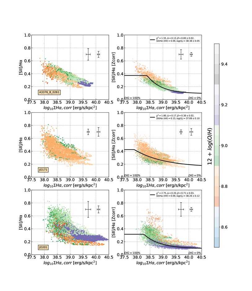
Figure 2: Left- The $\rm[S\textsc{II}]/H\alpha$ vs. $\rm\Sigma H\alpha,corr$ where we did not correct [SII]/H$\alpha$ values for metallicity variation. Right- The $\rm[S\textsc{II}]/H\alpha|_{Zcorr}$ vs. $\rm\Sigma H\alpha,corr$, where we did correct [SII]/H$\alpha$ values for metalicities that change with galactocentric radius. The values in all panels were color-coded by metallicity values that are median values of metallicities within bins of galactocentric radii. On right panels, we show fits on the data with the black lines. We present the median of uncertainties of all data with error-bar on the right, while the median of uncertainties of 5% spaxels with lowest $\rm\Sigma H\alpha,corr$ with error-bars on the left. Also, in the upper right corner, we write $\chi^{2}$ of the fit, 3$\sigma$ scatter in [SII]/H$\alpha$ of the data from the fitted line ($\Delta$), estimated $\beta$ and $\rm f_{0}$ values (and their 3$\sigma$ uncertainties), and the [SII]/H$\alpha$ of H II dominated spaxels. Values of $\rm f_{0}$ are in the units of surface brightness. Galaxies presented here are $A3376\_B\_0261$, JO171, and JO201. For details, see the text in Sec 3.

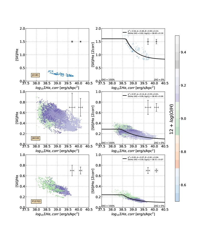
Figure 3: Same as Fig. 2, but for galaxies JO181, JW100 and P15703.

3 Estimating the diffuse ionized gas fraction

Estimating the distribution and the fraction of the diffuse ionized gas in each galaxy is hindered by the fact that generally the observed H$\alpha$ emission in the line of sight is composed of both the emission coming from regions of dense gas (non DIG) and from the DIG. The fraction of the total H$\alpha$ emission from the DIG and the dense gas is labeled as $\rm C_{DIG}$ and $\rm C_{dense}$, respectively, with a mutual relation $\rm C_{DIG}$ = 1 - $\rm C_{dense}$. Therefore, following Blanc et al. (2009) and Kaplan et al. (2016), we can empirically estimate $\rm C_{DIG}$ across a galaxy, and the total observed H$\alpha$ surface brightness along the LOS ($\rm\Sigma H\alpha,obs$) relate to the observed H$\alpha$ surface brightness from the DIG ($\rm\Sigma H\alpha,obs|_{DIG}$) as in the following equation:

$$\rm\Sigma H\alpha,obs=C_{dense}\cdot\Sigma H\alpha,obs+C_{DIG}\cdot\Sigma H\alpha,obs\;\;\;,$$ (1)

$$\rm\Sigma H\alpha,obs|_{DIG}=C_{DIG}\cdot\Sigma H\alpha,obs\;\;\;.$$ (2)

Blanc et al. (2009) and Kaplan et al. (2016) compared $\rm\Sigma(H\alpha,corr)$ and [SII]/H$\alpha$ line ratios and assumed a relation between the [SII]/H$\alpha$ ratios and $\rm C_{DIG}$ that depends on the gas phase metallicity:

$$\rm\frac{[S\textsc{II}]}{H\alpha}\Bigg{|}_{obs}=Z^{\prime}\left(C_{dense}\cdot\frac{[S\textsc{II}]}{H\alpha}\Bigg{|}_{dense,\,Zcorr}+C_{DIG}\cdot\frac{[S\textsc{II}]}{H\alpha}\Bigg{|}_{DIG,\,Zcorr}\right)$$ (3)

where $\rm[S\textsc{II}]/H\alpha|_{obs}$ is the observed line ratio in LOS, and $\rm[S\textsc{II}]/H\alpha|_{dense,\,Zcorr}$ and $\rm[S\textsc{II}]/H\alpha|_{DIG,\,Zcorr}$ are empirically determined for dense gas and DIG dominated spaxels, with the local ISM gas-phase metallicity. In the Milky Way, the H II regions (regions of dense gas) show $\rm[S\textsc{II}\,\lambda 6717]/H\alpha|_{H\,\textsc{II}}=0.11$ with a small scatter (standard deviation $\approx 0.03$), while the DIG regions show $\rm[S\textsc{II}\,\lambda 6717]/H\alpha|_{DIG}\approx 0.34$ with a large scatter (standard deviation $\approx 0.13$; Madsen et al. 2006). The Z^′ value is the ratio of the metallicity of the observed galaxies and the Milky Way ($\rm Z^{\prime}=Z_{gal}/Z_{MW}$). In this case, the Milky Way metallicity values are equivalent to the values of the ISM around the Sun (Grevesse et al. 1996).

Note that Blanc et al. (2009) and Kaplan et al. (2016) used one value of Z^′ per galaxy. This assumption is good enough when observations cover a relatively small area within galaxies, but would fail for observations covering the entire galaxies, including the debris tails outside the stellar disks, as in the case of GASP. Indeed, the strong metallicity variations observed across the galaxy disks (Franchetto et al. 2020, Franchetto in prep.) may drastically affect [SII]/H$\alpha$ line ratios and thus hinder a proper estimation of the $\rm C_{DIG}$.

3.1 Step-by-step estimation of $\rm C_{DIG}$

In this paper, we introduce a technique that accounts for metallicity variations within galaxies, unlike the technique previously used by Blanc et al. (2009) and Kaplan et al. (2016). Our technique considers the metallicity at each spaxel, including those in the tails: given the broad range in positions and physical conditions, metallicity might assume a large range. We describe in the following subsection the technique for measuring $\rm C_{DIG}$.

Even though we have gas-phase metallicity values for each spaxel separately, to reduce the noise, we used metallicities estimated in the following way. We divided the spaxels into annuli of different deprojected galactocentric radii, and estimated a median value of the spaxel metallicities (measured by Franchetto et al. 2020) for each individual radial annulus. Then we assigned to all the spaxels in a given annulus the same measured median metallicity. This metallicity value is used as radial metallicity ($Z_{gal}$) for spaxels in their corresponding radial bins, as shown by the colored points in Fig. 2 and 3.

In the first step, we divide the $\rm[S\textsc{II}]/H\alpha$ values by the corresponding $\rm Z^{\prime}$ ratio ($\rm Z^{\prime}=Z_{gal}/Z_{MW}$). We label these new values as $\rm[S\textsc{II}]/H\alpha|_{Zcorr}$. In the left panels of Fig. 2 and 3, we show $\rm[S\textsc{II}]/H\alpha$ vs. $\rm\Sigma H\alpha,corr$ for 6 selected galaxies. In the right panels, we present $\rm[S\textsc{II}]/H\alpha|_{Zcorr}$ as a function of H$\alpha,corr$, and color-coded the spaxels by radial metallicity. The relation 3 then becomes:

$$\rm\frac{[S\textsc{II}]}{H\alpha}\Bigg{|}_{Zcorr}=C_{dense}\cdot\frac{[S\textsc{II}]}{H\alpha}\Bigg{|}_{dense,\,Zcorr}+C_{DIG}\cdot\frac{[S\textsc{II}]}{H\alpha}\Bigg{|}_{DIG,\,Zcorr}\;\;\;.$$ (4)

As seen on the figure, the scatter of the data after the metallicity correction becomes smaller, thus improving estimation of the DIG fractions.

In the second step, we empirically estimate $\rm[S\textsc{II}]/H\alpha|_{DIG,\,Zcorr}$ and $\rm[S\textsc{II}]/H\alpha|_{dense,\,Zcorr}$ as the median value of 5% spaxels with lowest and highest value in $\rm\Sigma H\alpha,corr$, assuming that these extreme regimes are dominated by the DIG and dense gas respectively. Following the method from Kaplan et al. (2016), we compute a first empirical guess for $\rm C_{DIG}$ relation, which is directly derived from Eq. 4, as:

$$\rm C_{DIG}=\frac{[S\textsc{II}]/H\alpha|_{dense,\,Zcorr}-[S\textsc{II}]/H\alpha|_{Zcorr}}{[S\textsc{II}]/H\alpha|_{dense,\,Zcorr}-[S\textsc{II}]/H\alpha|_{DIG,Zcorr}}\;\;\;.$$ (5)

Finally, we fit these estimated $\rm C_{DIG}$ and $\rm\Sigma H\alpha,corr$, following an assumed relation between $\rm\Sigma H\alpha,corr$ and $\rm C_{DIG}$ (following Blanc et al. 2009 and Kaplan et al. 2016) as:

$$C_{DIG}=\Big{(}\frac{f_{0}}{\Sigma H\alpha,corr}\Big{)}^{\beta}\;\;\;.$$ (6)

This relation is valid only for $\rm\Sigma H\alpha,corr>f_{0}$. Here, $\rm f_{0}$ indicates the $\rm\Sigma H\alpha,corr$ value for spaxels with DIG-only emission ($\rm C_{DIG}=1$). In the case that $\beta$ is equal to 1, it would mean that the DIG surface brightness is constant across the galaxy ($\rm C_{DIG=\,f_{0}}$), which follows after combining Eq. 2 and 6. If the DIG is affected by the intensity of the dense gas, $\beta$ would be lower than 1.

The final fit on $\rm[S\textsc{II}]/H\alpha|_{Zcorr}$ values that correlate with $\rm C_{DIG}$ following Eq. 3 and 5 is shown as a thick line in the right panels of Fig. 2 and 3. We used the MPFIT (Markwardt 2009) model in python code for fitting the data. Here, the horizontal part of the line ($\rm\Sigma H\alpha,corr<f_{0}$) assumes the values in $\rm\Sigma H\alpha,corr$ with $\rm C_{DIG}=1$, while the part toward higher $\rm\Sigma H\alpha,corr$ corresponds to $\rm C_{DIG}=0$. In the upper right corners of the right panels, we write $\chi^{2}$ of the fit, 3$\sigma$ scatter in [SII]/H$\alpha$ of the data from the fitted line ($\Delta$), estimated $\beta$ and $\rm f_{0}$ values, and the [SII]/H$\alpha$ of dense gas dominated spaxels.

For each individual galaxy, we derive single values of $\rm f_{0}$ and $\beta$. Then, following Eq. 6, we use $\rm f_{0}$ and $\beta$ values on the $\rm\Sigma H\alpha,corr$ map to derive $\rm C_{DIG}$ in each spaxel. We show and discuss these maps in Sec. 4.1. Uncertainties in $\rm C_{DIG}$ for individual spaxels are estimated combining the uncertainties from different sources. These include errors on variables ($\rm f_{0}$ and $\beta$, as an output of the fit) and uncertainties of $\rm\Sigma H\alpha,corr$. An additional uncertainty is a difference between the $\rm C_{DIG}$ estimated using spaxel-by-spaxel metallicity and $\rm C_{DIG}$ estimated using metallicity that changes with galactocentric radius.

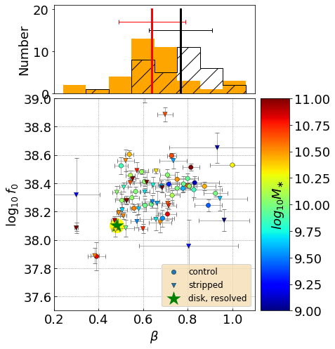
Figure 4: $\beta$ and $\rm f_{0}$ values for galaxies of the control sample (circles) and stripped galaxies (triangles), color-coded by stellar mass. The $\rm 3\sigma$ uncertainties are presented with error bars. The green star shows the result of the fit from the resolved data from the disks only (from Fig. 8). The histograms show the distribution of $\beta$ values for the control sample (white with lines) and for stripped galaxies (orange). The median $\beta$ value (and corresponding $1\,\sigma$ of distributions) for control (stripped) galaxies is presented with a black (red) line.

Table 1: Galaxies from the control sample, and their disk $\rm\Sigma SFR$, $\rm f_{0}$ and $\beta$ values (and their $\rm 3\sigma$ uncertainties), $\rm C_{DIG,\,disk}$ (uncertainty estimated as a mean of spaxel-by-spaxel $\rm C_{DIG}$ uncertainties), and the spatial fractions of spaxels that have $\rm C_{DIG}>0.3$ within the disk (uncertainties calculated assuming a bimodal distribution).

Name	$\rm\Sigma SFR_{disk}$	$\beta$	$\rm log_{10}f_{0}$	C$\rm{}_{DIG,\,disk}$	C$\rm{}_{DIG}>$0.3 spaxels
	[$\rm M_{\odot}/yr/kpc^{2}$]		[$\rm erg/s/kpc^{2}$]		Fraction of area
A3128_B_0148	0.0112	0.75 $\pm$ 0.04	38.36 $\pm$ 0.04	0.23 $\pm$ 0.04	0.69 $\pm$ 0.03
A3266_B_0257	0.0049	0.57 $\pm$ 0.02	38.34 $\pm$ 0.03	0.38 $\pm$ 0.07	0.83 $\pm$ 0.02
A3376_B_0261	0.0051	0.80 $\pm$ 0.02	38.38 $\pm$ 0.02	0.30 $\pm$ 0.06	0.71 $\pm$ 0.01
A970_B_0338	0.0070	0.54 $\pm$ 0.02	38.46 $\pm$ 0.03	0.37 $\pm$ 0.05	0.80 $\pm$ 0.02
JO102	0.0105	0.71 $\pm$ 0.03	38.46 $\pm$ 0.04	0.22 $\pm$ 0.05	0.57 $\pm$ 0.03
JO123	0.0027	0.78 $\pm$ 0.08	38.39 $\pm$ 0.05	0.56 $\pm$ 0.07	0.87 $\pm$ 0.02
JO128	0.0022	0.64 $\pm$ 0.03	38.25 $\pm$ 0.03	0.51 $\pm$ 0.07	0.93 $\pm$ 0.01
JO138	0.0030	0.69 $\pm$ 0.05	38.15 $\pm$ 0.06	0.39 $\pm$ 0.10	0.83 $\pm$ 0.02
JO159	0.0152	0.50 $\pm$ 0.03	38.52 $\pm$ 0.06	0.28 $\pm$ 0.03	0.86 $\pm$ 0.01
JO17	0.0051	0.59 $\pm$ 0.01	38.48 $\pm$ 0.02	0.44 $\pm$ 0.06	0.86 $\pm$ 0.01
JO180	0.0027	0.80 $\pm$ 0.05	38.43 $\pm$ 0.03	0.50 $\pm$ 0.07	0.86 $\pm$ 0.02
JO197	0.0063	0.61 $\pm$ 0.02	38.41 $\pm$ 0.03	0.33 $\pm$ 0.05	0.76 $\pm$ 0.02
JO205	0.0062	0.71 $\pm$ 0.05	38.39 $\pm$ 0.05	0.32 $\pm$ 0.04	0.80 $\pm$ 0.02
JO41	0.0020	1.00 $\pm$ 0.10	38.53 $\pm$ 0.01	0.88 $\pm$ 0.08	0.98 $\pm$ 0.01
JO45	0.0017	0.83 $\pm$ 0.11	38.40 $\pm$ 0.05	0.63 $\pm$ 0.08	0.97 $\pm$ 0.01
JO5	0.0039	0.73 $\pm$ 0.03	38.31 $\pm$ 0.04	0.34 $\pm$ 0.05	0.74 $\pm$ 0.01
JO68	0.0047	0.50 $\pm$ 0.03	38.28 $\pm$ 0.05	0.41 $\pm$ 0.05	0.86 $\pm$ 0.01
JO73	0.0038	0.55 $\pm$ 0.03	38.30 $\pm$ 0.04	0.43 $\pm$ 0.06	0.93 $\pm$ 0.01
JO89	0.0015	0.83 $\pm$ 0.12	38.35 $\pm$ 0.06	0.87 $\pm$ 0.14	0.98 $\pm$ 0.01
P13384	0.0050	0.61 $\pm$ 0.03	38.24 $\pm$ 0.04	0.32 $\pm$ 0.05	0.79 $\pm$ 0.01
P15703	0.0039	0.81 $\pm$ 0.04	38.51 $\pm$ 0.03	0.71 $\pm$ 0.08	0.89 $\pm$ 0.01
P17945	0.0045	0.78 $\pm$ 0.03	38.36 $\pm$ 0.03	0.32 $\pm$ 0.05	0.74 $\pm$ 0.02
P20769	0.0037	0.89 $\pm$ 0.06	38.24 $\pm$ 0.04	0.39 $\pm$ 0.07	0.80 $\pm$ 0.02
P20883	0.0022	0.92 $\pm$ 0.05	38.33 $\pm$ 0.02	0.46 $\pm$ 0.08	0.85 $\pm$ 0.02
P21734	0.0030	0.71 $\pm$ 0.04	38.18 $\pm$ 0.05	0.48 $\pm$ 0.06	0.81 $\pm$ 0.01
P25500	0.0025	0.39 $\pm$ 0.04	37.88 $\pm$ 0.10	0.69 $\pm$ 0.05	0.97 $\pm$ 0.00
P42932	0.0086	0.54 $\pm$ 0.02	38.60 $\pm$ 0.03	0.40 $\pm$ 0.04	0.85 $\pm$ 0.01
P45479	0.0067	0.73 $\pm$ 0.02	38.59 $\pm$ 0.02	0.40 $\pm$ 0.06	0.77 $\pm$ 0.01
P48157	0.0042	0.56 $\pm$ 0.02	38.22 $\pm$ 0.03	0.37 $\pm$ 0.05	0.83 $\pm$ 0.01
P57486	0.0043	0.81 $\pm$ 0.03	38.38 $\pm$ 0.03	0.30 $\pm$ 0.05	0.73 $\pm$ 0.02
P648	0.0028	0.88 $\pm$ 0.05	38.38 $\pm$ 0.03	0.55 $\pm$ 0.07	0.83 $\pm$ 0.01
P669	0.0022	0.75 $\pm$ 0.08	38.43 $\pm$ 0.05	0.84 $\pm$ 0.09	0.98 $\pm$ 0.00
P954	0.0035	0.68 $\pm$ 0.05	38.38 $\pm$ 0.04	0.45 $\pm$ 0.06	0.87 $\pm$ 0.01

Table 2: Stripped galaxies and their disk $\rm\Sigma SFR$, $\rm f_{0}$ and $\beta$ values, $\rm C_{DIG,\,disk}$, and the spatial fractions of spaxels that have $\rm C_{DIG}>0.3$ within the disk.

Name	$\rm\Sigma SFR_{disk}$	$\beta$	$\rm log_{10}f_{0}$	C$\rm{}_{DIG,\,disk}$	C$\rm{}_{DIG}>$0.3 spaxels
	[$\rm M_{\odot}/yr/kpc^{2}$]		[$\rm erg/s/kpc^{2}$]		Fraction of area
JO10	0.0599	0.70 $\pm$ 0.04	38.89 $\pm$ 0.05	0.17 $\pm$ 0.05	0.53 $\pm$ 0.03
JO112	0.0064	0.64 $\pm$ 0.06	38.39 $\pm$ 0.06	0.29 $\pm$ 0.05	0.73 $\pm$ 0.02
JO113	0.0139	0.51 $\pm$ 0.02	38.21 $\pm$ 0.04	0.50 $\pm$ 0.05	0.88 $\pm$ 0.01
JO13	0.0083	0.51 $\pm$ 0.02	38.37 $\pm$ 0.03	0.32 $\pm$ 0.04	0.79 $\pm$ 0.01
JO135	0.0070	0.68 $\pm$ 0.03	38.37 $\pm$ 0.03	0.33 $\pm$ 0.06	0.75 $\pm$ 0.01
JO141	0.0107	0.54 $\pm$ 0.02	38.40 $\pm$ 0.03	0.33 $\pm$ 0.05	0.76 $\pm$ 0.01
JO144	0.0327	0.52 $\pm$ 0.01	38.28 $\pm$ 0.03	0.13 $\pm$ 0.06	0.57 $\pm$ 0.02
JO147	0.0138	0.53 $\pm$ 0.01	38.28 $\pm$ 0.02	0.25 $\pm$ 0.05	0.76 $\pm$ 0.01
JO156	0.0027	0.66 $\pm$ 0.07	38.15 $\pm$ 0.08	0.41 $\pm$ 0.06	0.89 $\pm$ 0.01
JO160	0.0135	0.48 $\pm$ 0.02	38.34 $\pm$ 0.05	0.27 $\pm$ 0.04	0.73 $\pm$ 0.02
JO162	0.0051	0.57 $\pm$ 0.03	38.13 $\pm$ 0.05	0.29 $\pm$ 0.05	0.82 $\pm$ 0.02
JO171	0.0025	0.38 $\pm$ 0.02	37.89 $\pm$ 0.06	0.47 $\pm$ 0.05	0.96 $\pm$ 0.00
JO175	0.0114	0.49 $\pm$ 0.01	38.19 $\pm$ 0.02	0.21 $\pm$ 0.05	0.83 $\pm$ 0.01
JO179	0.0066	0.66 $\pm$ 0.07	38.26 $\pm$ 0.09	0.29 $\pm$ 0.06	0.82 $\pm$ 0.02
JO181	0.0059	0.93 $\pm$ 0.22	38.65 $\pm$ 0.11	0.56 $\pm$ 0.06	0.94 $\pm$ 0.02
JO194	0.0111	0.30 $\pm$ 0.01	38.08 $\pm$ 0.04	0.48 $\pm$ 0.03	0.97 $\pm$ 0.00
JO200	0.0024	0.71 $\pm$ 0.03	38.24 $\pm$ 0.03	0.78 $\pm$ 0.08	0.95 $\pm$ 0.00
JO201	0.0089	0.71 $\pm$ 0.03	38.26 $\pm$ 0.03	0.20 $\pm$ 0.06	0.76 $\pm$ 0.01
JO204	0.0070	0.60 $\pm$ 0.02	38.08 $\pm$ 0.03	0.25 $\pm$ 0.06	0.82 $\pm$ 0.01
JO206	0.0092	0.47 $\pm$ 0.01	38.14 $\pm$ 0.03	0.25 $\pm$ 0.05	0.86 $\pm$ 0.01
JO23	0.0085	0.64 $\pm$ 0.03	38.27 $\pm$ 0.05	0.22 $\pm$ 0.06	0.67 $\pm$ 0.04
JO27	0.0073	0.30 $\pm$ 0.10	38.32 $\pm$ 0.26	0.60 $\pm$ 0.06	1.00 $\pm$ 0.00
JO28	0.0020	0.80 $\pm$ 0.22	37.96 $\pm$ 0.19	0.35 $\pm$ 0.09	0.76 $\pm$ 0.02
JO36	0.2151	0.61 $\pm$ 0.09	39.09 $\pm$ 0.12	0.32 $\pm$ 0.07	0.62 $\pm$ 0.03
JO47	0.0025	0.58 $\pm$ 0.03	38.22 $\pm$ 0.04	0.48 $\pm$ 0.07	0.92 $\pm$ 0.01
JO49	0.0062	0.57 $\pm$ 0.05	38.49 $\pm$ 0.06	0.68 $\pm$ 0.05	0.93 $\pm$ 0.01
JO60	0.0131	0.48 $\pm$ 0.02	38.07 $\pm$ 0.05	0.34 $\pm$ 0.06	0.81 $\pm$ 0.01
JO69	0.0051	0.61 $\pm$ 0.02	38.34 $\pm$ 0.03	0.36 $\pm$ 0.05	0.86 $\pm$ 0.01
JO70	0.0062	0.66 $\pm$ 0.02	38.49 $\pm$ 0.02	0.39 $\pm$ 0.05	0.88 $\pm$ 0.01
JO85	0.0060	0.51 $\pm$ 0.01	38.17 $\pm$ 0.02	0.34 $\pm$ 0.04	0.87 $\pm$ 0.00
JO93	0.0033	0.68 $\pm$ 0.05	38.12 $\pm$ 0.07	0.61 $\pm$ 0.05	0.89 $\pm$ 0.00
JW10	0.0025	0.52 $\pm$ 0.04	38.08 $\pm$ 0.06	0.45 $\pm$ 0.07	0.91 $\pm$ 0.01
JW100	0.0074	0.55 $\pm$ 0.01	38.43 $\pm$ 0.02	0.41 $\pm$ 0.08	0.91 $\pm$ 0.00
JW108	0.0644	0.52 $\pm$ 0.04	38.56 $\pm$ 0.08	0.16 $\pm$ 0.04	0.61 $\pm$ 0.03
JW115	0.0056	0.94 $\pm$ 0.12	38.29 $\pm$ 0.09	0.30 $\pm$ 0.08	0.76 $\pm$ 0.03
JW29	0.0047	0.74 $\pm$ 0.06	38.56 $\pm$ 0.05	0.59 $\pm$ 0.05	0.94 $\pm$ 0.01
JW39	0.0032	0.62 $\pm$ 0.06	38.41 $\pm$ 0.07	0.87 $\pm$ 0.07	0.98 $\pm$ 0.00
JW56	0.0045	0.96 $\pm$ 0.11	38.14 $\pm$ 0.07	0.19 $\pm$ 0.10	0.85 $\pm$ 0.02

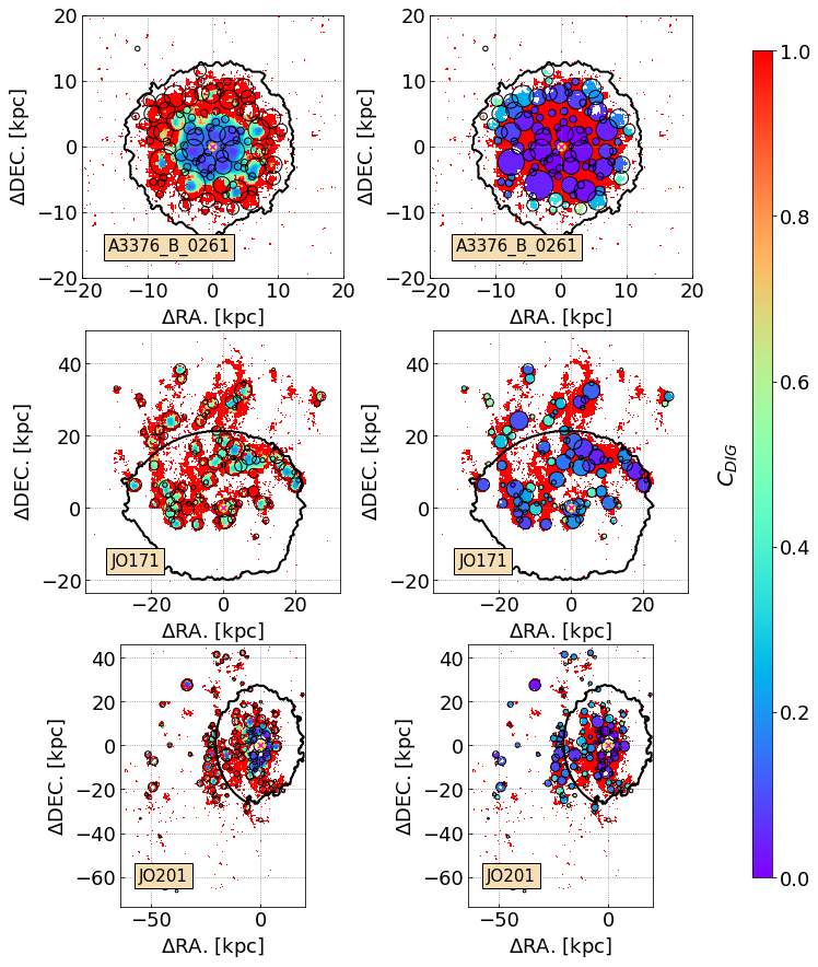
Figure 5: Left- Maps of emission fraction of the diffuse ionized gas ($\rm C_{DIG}$), based on the method used in this paper.We present location and sizes of $\rm H\alpha$ clumps (estimated in Poggianti et al. 2017a) with black circles. Right- Maps of the fraction of background diffuse emission previously estimated for the clumps. For definition of the background diffuse emission, see Sec. 4.1. In each map, we indicate the stellar disk (thick, black contour; Gullieuszik et al. 2020), and galactic center (magenta cross on yellow circle). Galaxies presented here are $A3376\_B\_0261$, JO171, and JO201.

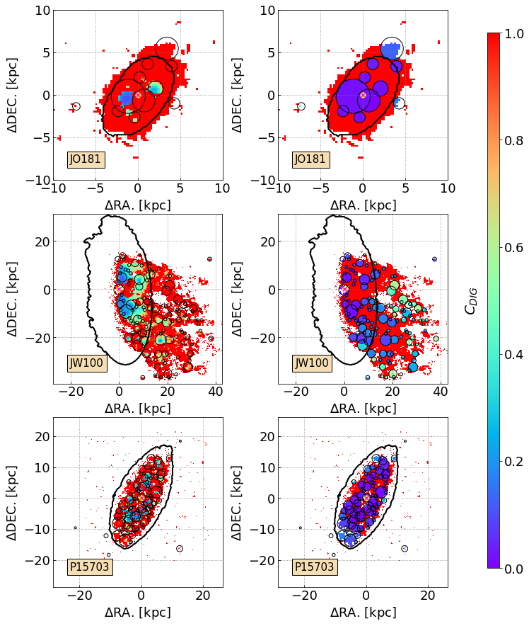
Figure 6: Same as Fig. 5 but for galaxies JO181, JW100, and P15703.

3.2 Potential drawbacks

Due to the kpc-scale resolution of the analyzed emission-line maps (pixel size $\approx 200$ pc, and smoothing of the data using kernels $\approx 1$ kpc in size), we cannot resolve individual HII regions as done in other works (Blanc et al. 2009, Kreckel et al. 2016, Kaplan et al. 2016, etc.). Thus in each spaxel we expect contributions from both the DIG and the dense gas emission along the LOS. This implies that spaxels dominated by dense gas emission cannot reach exactly $\rm C_{DIG}=0$ values, but converge towards them. However, the anti-correlation between [SII]/H$\alpha$ and $\rm H\alpha,corr$ seen in our data is clear enough to estimate $\rm C_{DIG}$ values.

Applying this technique at lower spatial resolution would decrease the precision of the $\rm C_{DIG}$ determination. If single HII regions can be resolved instead, even other techniques, which use only $\rm H\alpha,corr$, or only [SII]/H$\alpha$ ratio, or equivalent width of $\rm H\alpha$ could suffice in separating DIG and dense gas dominated regions, and in estimating DIG properties.

One assumption that we applied in Sec. 3.1 is that the DIG emission has the same [SII]/H$\alpha$ ratio at the same metallicity. We note that this assumption is not strictly correct because the DIG shows a wide range of [SII]/H$\alpha$ ratios at specific metallicities (standard deviation $\approx 0.13$; Madsen et al. 2006). This increases the scatter in [SII]/H$\alpha$ of our data and introduces an additional uncertainty in the estimate of $\rm C_{DIG}$.

Another drawback of our approach is that the metallicity values were measured using the PYQZ code that assumes that the line emission (and thus line ratios) come only from ionization due to star-forming regions. PYQZ does not yet have a prescription for the line ratios in the DIG that have different physical conditions compared to the H II regions. Thus, this may add to uncertainties in measuring the metallicities, especially in the DIG emission dominated spaxels.

Furthermore, the metallicity radial gradient is not always symmetrical across the galaxies (A. Franchetto et al. in prep) due to inflows and morphological asymmetries in the disks and tails. At a given galactocentric radius, we also assume that corresponding spaxels dominated by the DIG and dense gas emission have the same metallicity which may not be correct. The assumption in Sec. 3 that in every galaxy we are able to always observe spaxels completely dominated by DIG emission, may not be correct. In this case, we would be slightly overestimating the DIG fraction. All the caveats discussed above in principle add to the scatter in the $\rm[S\textsc{II}]/H\alpha|_{Zcorr}$ values.

4 Results

Following the fitting method described in Sec. 3.1, using the spaxels from both the disks and tails, we estimated single $\beta$ and $\rm f_{0}$ values for each galaxy. These values are presented in Tab. 1 and 2, and shown in Fig. 4. Stripped galaxies have a statistically lower estimated $\beta$ (median 0.1 lower) compared to the control sample, but cover a similar range in $\rm f_{0}$.

In what follows, we will investigate the $\rm C_{DIG}$ maps, testing how $\rm C_{DIG}$ spaxel values (from disks of control sample and stripped galaxies) compare to values of $\rm\Sigma H\alpha,corr$, [SII]/H$\alpha$ line ratio, and $\rm W_{H\alpha}$, in order to understand if we can use a single threshold value of those quantities to separate spaxels dominated by emission from DIG and dense gas, as typically done in other works (Blanc et al. 2009, Kaplan et al. 2016). Furthermore, we will compare integrated $\rm C_{DIG}$ with other galactic properties, for stripped and control sample galaxies.

4.1 $\rm C_{DIG}$ maps

The $\rm C_{DIG}$ maps for six representative galaxies are presented in the left panels of Figs. 5 and 6, while those of the rest of the sample are shown in Appendix A. We also over-plot the $\rm H\alpha$ clumps described in Sec. 2.4. We remind the reader that these clumps detect peaks in $\rm H\alpha$ emission maps, and were not designated to measure fraction of emission from the DIG. However, a single galactic value of the background diffuse emission outside the clumps has been previously estimated as a median value of $\rm H\alpha$ surface brightness outside the clumps (Poggianti et al. 2017a). The fraction of $\rm H\alpha$ flux within the clumps that come from the background diffuse $\rm H\alpha$ emission is show in the right panels of Figs. 5 and 6.

The $\rm C_{DIG}$ maps indicate that the values within the clumps are typically higher than fractions of the background diffuse $\rm H\alpha$ emission. We also notice that the $\rm H\alpha$ clumps have large radii, typically extending beyond the region that is defined as dense gas according to our method.

We now compare the fractions of the DIG emission in the clumps with their fractions of background diffuse emission considering the 5202 clumps from all galaxies in the sample (control+stripped), both from the disks and the tails.

Fig. 7 shows that in clumps $\rm C_{DIG}$ values are higher (by a factor of $\approx 5$) than the fractions of background diffuse emission. The difference ranges from below 0.1 for the dense gas dominated clumps, to 0.8 in the DIG dominated clumps.

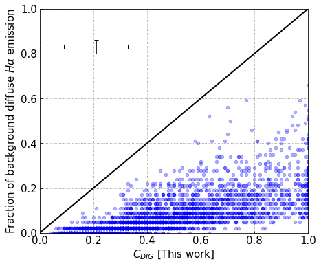
Figure 7: Comparison of the $\rm H\alpha$ clumps between the $\rm C_{DIG}$ values (x-axis) and the fractions of background diffuse emission (y-axis). For definition of the background diffuse emission, see Sec. 4.1. Median uncertainties are presented by the error bars, and $1:1$ relation is presented by the thick black line. There are 4410 clumps in total.

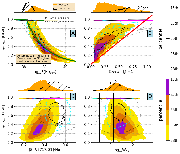
Figure 8: Spatially resolved spaxel data (323340 spaxels in total) from the disks of all galaxies. The colored regions indicate spaxels that are designated as star-forming by the BPT diagram utilising $\rm[O\textsc{i}]/H\alpha$ line ratio, while the line-contour show non star-forming spaxels. The contours represent the 15th, 35th, 65th, 85th and 98th percentiles. Above each panel, we show a histogram of spaxels that have $\rm C_{DIG}=1$. Filled (empty) histograms are for star-forming (non star-forming) spaxels. Panel A: $\rm C_{DIG}$ as a function of $\rm H\alpha_{corr}$ surface brightness. The fitted relation, following Eq. 6 is shown with the green line. Panel B: Comparison between estimated $\rm C_{DIG}$ and the $\rm C_{DIG}$ calculated with $\beta=1$ and the $\rm f_{0}$ that is a result of the fit in the upper-left panel. The thick red line represents 1:1 relation. Panel C: $\rm C_{DIG}$ as a function of $\rm[S\textsc{II}]/H\alpha$ ratio. Panel D: $\rm C_{DIG}$ as a function of equivalent width $\rm W_{H\alpha}$. $\rm W_{H\alpha}$ equal to 3 Å  and 14 Å  are indicated by the thick, black lines.

4.2 Spaxel by spaxel comparison

In Fig. 8 we investigate how $\rm C_{DIG}$ values from spatially resolved spaxels behave as a function of $\rm H\alpha_{corr}$, $\rm[S\textsc{II}]/H\alpha$, and $\rm W_{H\alpha}$ and inspect if the $\rm[O\textsc{i}]$-BPT diagram can distinguish spaxels dominated by the dense gas and the DIG emission. With the colored regions, we indicate spaxels that are designated as star-forming by the $\rm[O\textsc{i}]$-BPT diagram, while with the line-contour we show non star-forming spaxels. Above each panel, we show filled (empty) histograms of star-forming (non star-forming) spaxels that have $\rm C_{DIG}=1$. Here, we plot only spaxels from the disks.

In Panel A of Fig. 8 we present $\rm C_{DIG}$ as a function of $\rm\Sigma H\alpha_{corr}$. We fitted all the data following Eq. 6, which results in $\rm\beta=0.48$ and $\rm f_{0}=1.51\,\times\,10^{38}$ $\rm erg/s/kpc^{2}$. $\rm C_{DIG}$ has a large scatter ($\rm\Delta C_{DIG}\approx 0.28$), therefore using only this best fit $\rm H\alpha_{corr}$ relation can lead to errors on $\rm C_{DIG}$ estimates up to 40%.

The contours show that both the star-forming and non-star-forming spaxels show a large range in $\rm\Sigma H\alpha_{corr}$ and in $\rm C_{DIG}$. The spaxels with $\rm C_{DIG}=1$ (histograms in Fig. 8) also show a large range in $\rm\Sigma H\alpha_{corr}$ (up to 1.5 dex), with star-forming having slightly higher values. The star-forming and non star-forming contours overlap in almost the entire range of $\rm C_{DIG}$ and $\rm H\alpha_{corr}$.

In Panel B we consider a case where we apply $\beta=1$ and the $\rm f_{0}$ that is a result of the fit in the upper-left panel. Here we estimated $\rm C_{DIG}$ values by applying Eq. 6 on the $\rm\Sigma H\alpha_{corr}$ spaxel values, assuming $\beta=1$ and a single $\rm f_{0}$ value. The purpose of this plot is to test whether the assumption that the DIG surface brightness is constant across the galaxy/ies (thus $\beta=1$), and that using a single $\rm H\alpha_{corr}$ threshold value (single $\rm f_{0}$) would yield different results in $\rm C_{DIG}$ compared to our method. There is a large offset between those values and our estimated $\rm C_{DIG}$ values, suggesting that the hypothesis of $\beta=1$ is not reliable.

Comparing the spaxel-by-spaxel distributions of $\rm C_{DIG}$ for the stripped galaxies and the control sample (upper panel in Fig. 9), we find that the two distributions are similar and cover the same ranges. It is important to note that spaxels dominated by DIG or by dense gas, respectively, do not necessarily correspond to non star-forming vs star-forming spaxels. In Panel C of Fig. 8, it is clearly seen that star-forming spaxels preferentially have lower $\rm C_{DIG}$ than non star-forming spaxels. However, even star-forming spaxels can have a $\rm C_{DIG}=1$, and non star-forming spaxels can reach low $\rm C_{DIG}$ values. Thus, the dichotomy $\rm C_{DIG}$ vs. dense gas does not correspond necessarily to the distinction non star-forming vs star-forming. Even regions dominated by DIG can have star formation as dominant ionization source according to the $\rm[O\textsc{i}]$-BPT diagram. The partial overlap of the star-forming and the non-star-forming points might be related to the fact that even in regions that appear to be dominated by one ionization mechanism or another (based on the BPT diagram) there is probably a contribution from different ionization mechanisms (as discussed previously by Poggianti et al. 2019a).

The same panel displays $\rm C_{DIG}$ values as a function of $\rm[S\textsc{II}]/H\alpha$ ratio. As expected, $\rm C_{DIG}$ shows a correlation with $\rm[S\textsc{II}]/H\alpha$. The data shows a large scatter, thus making a single fit not viable. Furthermore, there is a large overlapping area (both in $\rm C_{DIG}$ and $\rm[S\textsc{II}]/H\alpha$) between star-forming and non star-forming distributions. The spaxels with $\rm C_{DIG}=1$ cover the $\rm 0.2<[S\textsc{II}]/H\alpha<0.7$ range.

In Panel D of Fig. 8, we compare $\rm W_{H\alpha}$ with $\rm C_{DIG}$. We indicate $\rm W_{H\alpha}=3$ Å  and $\rm W_{H\alpha}=14$ Å  values, which are given by Lacerda et al. (2018) to separate spaxels dominated by DIG emission from ones dominated by dense gas emission. The plot shows that most spaxels ($68\%$) have $\rm W_{H\alpha}>14$ Å , while some ($30\%$) have 3 Å$\rm<W_{H\alpha}<14$ Å. We do not see a significant difference in distribution of $\rm W_{H\alpha}$ for spaxels with $\rm C_{DIG}=1$ and the rest of spaxels.

The main conclusions that we draw from these results are: 1) each galaxy shows different $\beta$ and $\rm f_{0}$ values, 2) we cannot assume that $\beta=1$, or that the DIG $\rm H\alpha$ emission is constant in surface brightness across galaxies, 3) we cannot use a single $\rm H\alpha_{corr}$ value, or a single $\rm[S\textsc{II}]/H\alpha$ value, or a single $\rm W_{H\alpha}$ value to separate spaxels dominated by emission from the dense gas from the DIG, and 4) the BPT criteria identifying the source of ionisation (star formation vs no-star formation) cannot distinguish between spaxels dominated by the dense gas or the DIG emission.

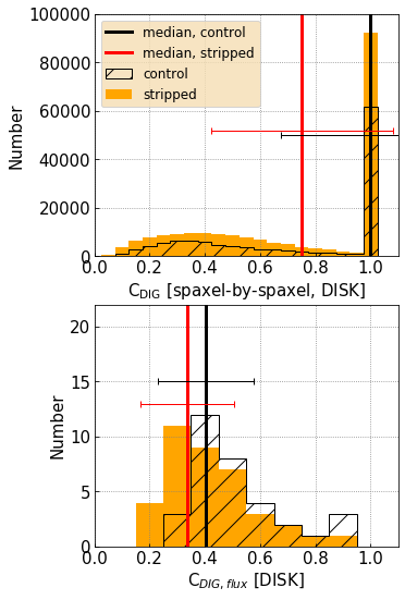
Figure 9: Histograms of disk spaxel-by-spaxel $\rm C_{DIG}$ values (upper panel) or integrated values of the disks ($\rm C_{DIG,\,disk}$; bottom panel) of control sample (empty histogram, with diagonal lines) and stripped galaxies (orange filled histogram). We present median values (and corresponding $1\,\sigma$ of distributions) with red (black) lines for the control (stripped) galaxies data.

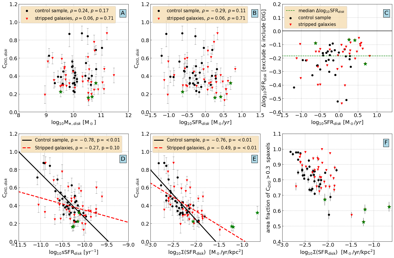
Figure 10: Fraction of integrated $\rm H\alpha$ surface brightness coming from the DIG ($\rm C_{DIG,\,disk}$) as a function of the stellar mass (panel A), total SFR of the disk ($\rm SFR_{disk}$; panel B), difference in $\rm SFR_{disk}$ (subtracting SFR after and SFR before removal of the DIG emission; panel C), sSFR (panel D), mean surface density of SFR ($\rm\Sigma SFR$; panel E). We separate and fit the data into the control sample (black circles), and stripped galaxies (red triangles), and label Pearson’s correlation coefficients and corresponding p-values. In the panels E, the figure shows area fraction of spaxels that have $\rm C_{DIG}>0.3$ (y axis), as a function of $\rm\Sigma SFR_{disk}$. Uncertainties in values of area fraction are calculated using error estimation of a bimodal distribution. We add a mean of the area fraction of star-forming spaxels for the control (stripped) data as the black (red) vertical line. We mark galaxies with truncated disk (JO10, JO23, JO36 and JW108) with large green star symbols.

4.3 Integrated DIG fraction

Using the derived $\rm C_{DIG}$, and multiplying them with the $\rm\Sigma H\alpha$ maps, we derived maps of the DIG surface brightness ($\rm\Sigma H\alpha_{DIG}$). We estimated then the fraction of the DIG emission within the disks ($\rm C_{DIG,\,disk}$) of all galaxies (control sample and stripped galaxies) as a ratio of integrated $\rm\Sigma H\alpha_{DIG}$ and integrated $\rm\Sigma H\alpha$. Here, we only use data from the disks in order to avoid the introduction of biases, due to the tails of the stripped galaxies. The galactic stellar masses ($\rm M_{\ast}$) and SFR are presented in Vulcani et al. (2018). We then compute the specific Star Formation Rate (sSFR) as SFR/$M_{\star}$.

In Fig. 10, we plot $\rm C_{DIG,\,disk}$ as a function of $\rm M_{\ast}$ (panel A), SFR of the disk ($\rm SFR_{disk}$, panel B), sSFR (panel D), and mean surface density of SFR ($\rm\Sigma SFR_{disk}$) of spaxels (panel E). We remind the reader that we define spaxels dominated by emission from the DIG as those which have $\rm C_{DIG}>0.3$. The difference in $\rm SFR_{disk}$ values (Panel C) is calculated by dividing the SFRs of spaxels where the DIG emission was removed, and the SFRs of spaxels with combined emission from the DIG and the dense gas.

The figure also shows the fraction of area dominated by DIG emission (area of all spaxels with H$\alpha$ emission), as a function of $\rm\Sigma SFR_{disk}$ (panel F). Here, we define spaxels dominated by the DIG emission if their $\rm C_{DIG}$ is greater than 0.3. This is an arbitrary choice, and changing it to higher number (for example $\rm C_{DIG}=0.6$) does not change results. We present the values of those data in Tab. 1 and 2. We separate the data between the control sample and stripped galaxies, and add Pearson’s correlation coefficients ($\rho$) to certain trends.

The disk integrated $\rm C_{DIG,\,disk}$ values range between 0.2 and 0.9, indicating that the DIG flux contributes from 20% to 90% in the galaxy disks. Stripped and control sample galaxies cover a similar range in $\rm C_{DIG,\,disk}$, as also seen in bottom panel of Fig. 9). The Kolmogorov-Smirnov test on those samples results in p-value of 5.8%, thus indicating that those two samples come from a same population.

We do not see any trend between $\rm C_{DIG,\,disk}$ and the stellar mass or SFRs (Panels A and B), as indicated by relatively low Pearson’s coefficients ($|\rho|<0.3$). As expected, subtracting the DIG emission lowers $\rm SFR_{disk}$ by $\approx$0.2 dex (Panel C).

On the other hand, $\rm C_{DIG,\,disk}$ seems to anti-correlate with sSFR (Panel D), when all galaxies are considered. The control sample galaxies show a strong correlation ($|\rho|\approx 0.78$) compared to the stripped galaxies($|\rho|\approx 0.27$), with trends :

$$\rm C_{DIG,\,disk}=(-0.48\pm 0.07)\cdot log_{10}sSFR+(-4.6\pm 0.7)$$ (7)

for the control sample, and

$$\rm C_{DIG,\,disk}=(-0.14\pm 0.08)\cdot log_{10}sSFR+(-1\pm 0.8)$$ (8)

for the stripped galaxies.

There is a clear correlation also between $\rm C_{DIG,\,disk}$ and $\rm\Sigma SFR_{disk}$ (Panel E), with high Pearson’s coefficients ($\rho=-0.5$ and $\rho=-0.7$ for stripped and control galaxies). For the fit, we excluded galaxies with truncated disks (JO10, JO23, JO36 and JW108; marked as green stars). These anti-correlations (fitted using MPFIT; Markwardt 2009) are as follows:

$$\rm C_{DIG\,disk}=(-0.56\pm 0.09)\cdot log_{10}\Sigma SFR+(-0.9\pm 0.2)$$ (9)

for the control sample, and

$$\rm C_{DIG\,disk}=(-0.31\pm 0.09)\cdot log_{10}\Sigma SFR+(-0.3\pm 0.1)$$ (10)

for the stripped galaxies.

Generally, the data from both types of galaxies cover a similar area on the diagram, though the stripped galaxies show a larger scatter. The data points indicate that the stripped galaxies show slightly higher $\rm C_{DIG,\,disk}$ values at high $\rm\Sigma SFR_{disk}$, but cover a similar range in $\rm C_{DIG,\,disk}$ at low $\rm\Sigma SFR_{disk}$.

The area fraction of the DIG dominated spaxels indicate higher values for the stripped galaxies at a given $\rm\Sigma SFR_{disk}$, compared to the control sample (panel E in Fig. 10). That indicates that, at a given $\rm\Sigma SFR_{disk}$, the spaxels dominated by emission from the DIG cover a larger fraction of the area in stripped galaxies, compared to control galaxies.

5 Discussion

Here we comment on how the $\rm C_{DIG}$ measuring technique used in this paper, which utilises both the $\rm H\alpha$ surface brightness and the [SII]/H$\alpha$ ratio, differs from other methods used in the literature, and we discuss the benefits of our method. We also discuss variations and trends in integrated $\rm C_{DIG,\,disk}$ among the galaxies.

5.1 Methods based only on H$\alpha$ or [SII]/H$\alpha$ ratio, and spaxel-by-spaxel comparison

Previous spatially resolved studies used methods of estimating the DIG distribution and fractions that assume only a certain threshold in H$\alpha$ surface brightness, or assume a threshold in [SII]/H$\alpha$ line ratio (Oey et al. 2007, Kreckel et al. 2016, Zhang et al. 2017, Poetrodjojo et al. 2019, Kumari et al. 2019, den Brok et al. 2020). This is possible when a spatial resolution (spaxels sizes $\rm<50$ pc) enables to resolve individual HII regions and their association, such as in Kreckel et al. (2016). However, this is not possible at lower spatial resolutions.

Our results indicates that we cannot use a single value in H$\alpha$ surface brightness or [SII]/H$\alpha$ to separate spaxels dominated by DIG or the dense gas as seen in Fig. 8. For example, previously used H$\alpha$ clumps were determined using only H$\alpha$ maps, but it resulted in fractions of the background diffuse emission within those clumps to be underestimated compared to the $\rm C_{DIG}$ values. In conclusion, combining information from both the H$\alpha$ surface brightness and [SII]/H$\alpha$ line ratios, the determined $\rm C_{DIG}$ should be measured more precisely and avoid the main drawbacks of previously used methods.

Although there is a spaxel-by-spaxel correlation between $\rm C_{DIG}$ and $\rm\Sigma H\alpha,corr$ due to the relation seen in Eq. 6, there is a relatively large scatter caused by variations among the galaxies and their values of $\beta$ and $\rm f_{0}$.

Our results also indicate that we cannot use the same $\beta$ and $\rm f_{0}$ value for spatially resolved data of different galaxies (upper-right panel in Fig. 8).

5.2 $H\alpha$ Equivalent width

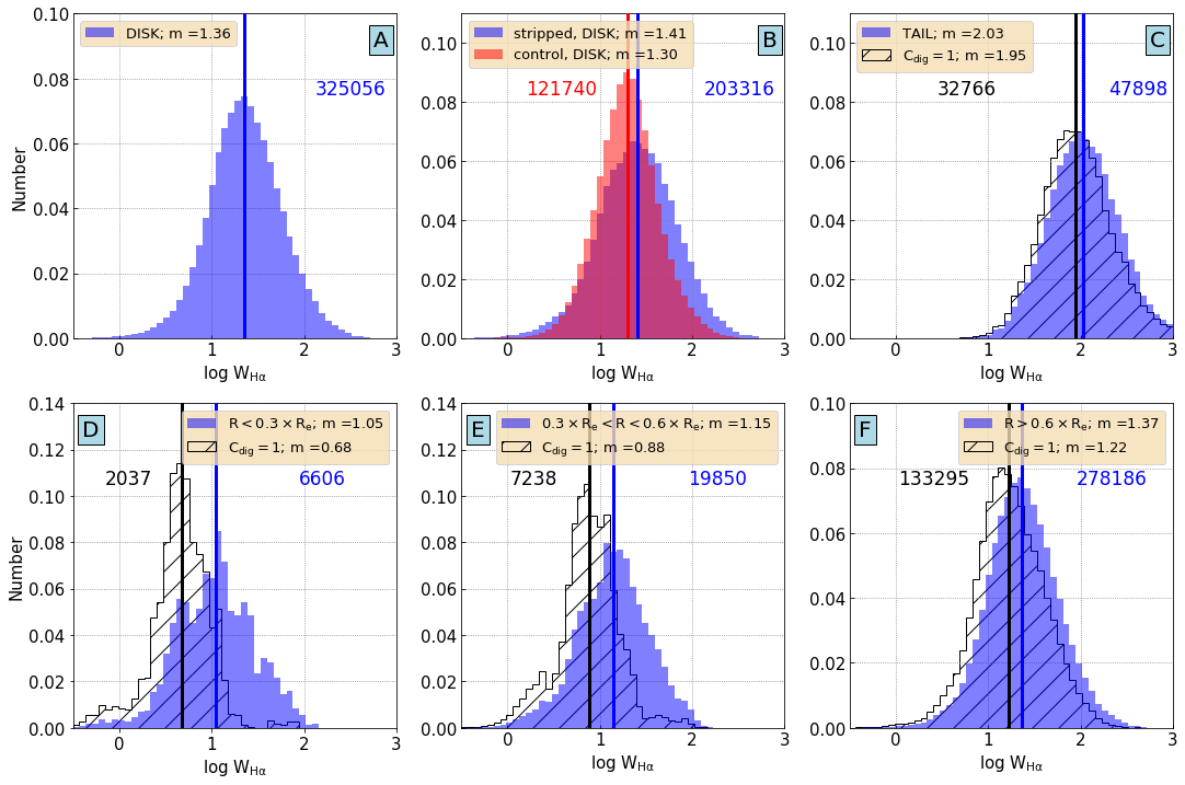
Figure 11: Histograms of H$\alpha$ equivalent width ($\rm W_{H\alpha}$) for all spaxels in: all disks (panel A), stripped (blue) and control (red) galaxies (panel B), tails (blue histogram in panel C). In panels D, E and F we show $\rm W_{H\alpha}$ values of disk spaxels with blue histograms, separated in 3 bins of different galactocentric radii. In Panels C, D, E and F, we added hatched histograms showing a sub-set of corresponding spaxels that have $\rm C_{DIG}=1$. We present also median values (labeled ’m’ in the legends) of corresponding histograms with lines of the same color. We show numbers of spaxels of each histogram next to corresponding histograms.

Some previous studies applied $\rm W_{H\alpha}\leqslant 3$ Å  (up to $\rm W_{H\alpha}\leqslant 14$ Å ) to disentangle spaxels dominated by emission from DIG and spaxels dominated by emission from the dense gas (Lacerda et al. 2018, Vale Asari et al. 2019, Vale Asari & Stasińska 2020, Mingozzi et al. 2020). There, spaxels that probe gas outside the star-forming regions (with low H$\alpha$ equivalent width) are dominated by ionization from Hot Low-Mass Evolved Stars (HOLMES; Stasińska et al. 2008, Flores-Fajardo et al. 2011b), thus having a low $\rm W_{H\alpha}$.

While the lower limit of 3 Å  in $\rm W_{H\alpha}$ is physically motivated (see Cid Fernandes et al. 2011), the upper limit of $\rm W_{H\alpha}=14$ Å  is purely empirical and depends on the spatial resolution of the observations. In order to evaluate these criteria in our sample of MUSE datacubes, in Fig. 11, we show histograms of $\rm W_{H\alpha}$ values in disks, stripped vs. control sample, tails and spaxels at different galactocentric distances. We also separate data from the disks and tails, to see if tails yield different results from the disks. As seen on the top row of panels Fig. 11, the peak of the $\rm W_{H\alpha}$ distribution of disk spaxels in our overall sample (panel A) is at 22.9 Å. Considering only the control sample (red histogram in panel B), which is more comparable to the CALIFA and MaNGA samples of Lacerda et al. (2018) and Vale Asari et al. (2019) the peak is at 19.0 Å, larger than the 14 Å  limit found in their works, which is expected due to the higher spatial resolution of MUSE data.

In the bottom-right panel of Fig. 8 we already showed that using only $\rm W_{H\alpha}$ does not allow us to clearly discriminate DIG and dense gas. This can also be seen in Fig. 11. $\rm W_{H\alpha}$ tends to span a large range in values (3-1000 Å), and we cannot distinguish DIG dominated from non-DIG dominated spaxels only using $\rm W_{H\alpha}$ distribution from the disks. There is no significant difference between stripped galaxies and control sample. However, a small difference between those samples may be caused by slightly higher spatially resolved $\rm\Sigma SFR$ of the stripped galaxies compared to control sample (Vulcani et al. 2020), thus resulting in slightly higher $\rm W_{H\alpha}$.

Overall, central regions have lower $\rm W_{H\alpha}$, similar to what is observed in nearby galaxies by Lacerda et al. (2018) and Vale Asari et al. (2019), while in the rest of the disk, $\rm W_{H\alpha}$ increases with galactocentric distance. We also notice that the DIG dominated spaxels in the disks mostly show slightly lower $\rm W_{H\alpha}$ compared to the rest of data in the same radial bin. However, if we only use histograms of all $\rm W_{H\alpha}$ values to distinguish DIG dominated spaxels from the rest, we are able to do it only in the central regions (Panel D, and partly Panel E). In the centers, the DIG dominated spaxels have $\approx 0.3$ dex lower $\rm W_{H\alpha}$ compared to the rest of data, a trend similarly seen by Lacerda et al. (2018).

The method from Lacerda et al. (2018) is not suited for the debris tails of the stripped galaxies. In the tails, $\rm W_{H\alpha}$ is $\approx 0.6$ dex higher than in the disks, and there is no difference between DIG dominated and non-DIG dominated spaxels. The tails of the gas-stripped galaxies do not have stars older than a few times $10^{8}$ yr, and its light is mostly dominated by a bright gas emission and younger stellar populations ($\rm<2-300$ Gyr, traced by ultra-violet emission; Bellhouse et al. 2017, George et al. 2018). This would drastically increase $\rm W_{H\alpha}$. Thus, equivalent width would be an unreliable estimator of the DIG and its fraction in the GASP galaxies, especially outside their disks.

To conclude, the variation in $\rm W_{H\alpha}$ is not caused only by an increase in $\rm C_{DIG}$, but also potentially by other sources. Therefore, we cannot prescribe a simple method of measuring $\rm C_{DIG}$ from $\rm W_{H\alpha}$, especially in the tails of stripped galaxies. Moreover, the kpc-scale spatial resolution of our data may also affect these measurements, due to combining regions with both low and high $\rm W_{H\alpha}$ in the LOS.

5.3 Integrated DIG correlations

Our results of integrated disk data show that the DIG contributes to a large fraction of the total H$\alpha$ flux ($\rm C_{DIG,\,disk}$) in galactic disks (between 20% and 90%; Fig. 9 and 10). This is similar to the range found in many other studies, where the DIG fraction was found to contribute between 30% and 80% (with mean values around 50%-60%; Hoopes & Walterbos 2003, Oey et al. 2007, Sanders et al. 2017, Poetrodjojo et al. 2019, Della Bruna et al. 2020).

In this work, we present for the first time a comparison between the stripped galaxies, and the control sample that are non-stripped galaxies. Also, for the first time, we compare integrated $\rm C_{DIG,\,disk}$ with global galactic values such as stellar mass, SFR, and $\rm sSFR_{disk}$.

On one hand, we do not see trends between the DIG fraction and the galactic stellar mass, or SFR. Vulcani et al. (2018) found a 0.2 dex difference in integrated SFR-M_∗ relation between stripped and control samples of galaxies. This difference in SFR-M_∗ relation would still exist if we subtract the DIG emission because the integrated SFR values would similarly decrease for both the stripped and control samples (Panel C in Fig. 10).

On the other hand, we detect anti-correlations with $\rm sSFR_{disk}$ and $\rm\Sigma SFR_{disk}$. The control sample shows stronger anti-correlation compared to the stripped galaxies. These anti-correlations potentially enables to robustly, but not precisely, measure fraction of the DIG emission in galactic disks by simply using $\rm sSFR_{disk}$ or $\rm\Sigma SFR$ values.

Oey et al. (2007) and Sanders et al. (2017) found a similar anti-correlation between the fraction of the DIG and $\rm\Sigma H\alpha$. Oey et al. (2007) defined borders of bright H$\alpha$ regions as borders of dense gas regions and a background emission (constant in $\rm\Sigma H\alpha$) as a DIG emission, while Sanders et al. (2017) designated spaxels within the first 10th percentile of $\rm\Sigma H\alpha$ distribution as DIG dominated spaxels. Furthermore, to explain spaxel-by-spaxel variation in dust attenuation and its effects on measuring Balmer line emission, Vale Asari et al. (2020) speculated that galaxies with lower $\rm sSFR_{disk}$ should have larger fraction of the DIG, the trend that we see for the galaxies in our sample. Since $\rm sSFR_{disk}$ can be used as an age indicator of stellar population, this result may indicate a correlation between the DIG fraction and the amount of old stellar population such as HOLMES (ages of above $10^{8}$ yr; Flores-Fajardo et al. 2011a), and could explain slightly stronger correlation in the case of the control sample. In other words, ionization from the older stellar population may contribute to ionization of the DIG.

At a given $\rm\Sigma SFR_{disk}$, the stripped galaxies have higher fraction of area covered by DIG dominated spaxels than the control sample. That may indicate two possible conclusions: 1) the DIG is brighter in surface brightness (higher $\rm\Sigma SFR_{disk}$) in the stripped galaxies at a given area fraction, or 2) the dense gas areas are smaller in size for the stripped galaxies compared to the control sample.

When we compare $\beta$ and $\rm f_{0}$ values for individual galaxies (Fig. 4), we notice that the stripped galaxies have median of $\beta\approx 0.1$ lower compared to the control sample, despite that they cover a large range ($\beta$ from 0.2 to 1). This may indicate that the DIG emission in galaxies (and even more in stripped galaxies) is not a constant in surface brightness across the disks. On what does its emission depend (on the $\rm H\textsc{II}$ regions, environment, and/or other sources) will be investigated in future papers.

6 Summary

The diffuse ionised gas (DIG) is an important component of the ISM that is affected by physical processes across the galaxies and their evolution. Measuring its distribution and fraction in surface brightness allows us to properly study its source of ionization and star formation in galaxies. Subtracting the DIG emission from the observed galactic images would remove biases from observations of the star formation and gas-phase metallicities.

In this paper, we measure for the first time the DIG emission in gas-stripped galaxies at different stages of gas-stripping, and compare them to normal galaxies. We utilise the IFU (MUSE spectrograph) observations of galaxies from the multi-wavelength project GASP, and study 71 galaxies. We used emission line maps to estimate the fraction of emission from the DIG ($\rm C_{DIG}$) using both the H$\alpha$ and [SII]/H$\alpha$ line ratios (Sec. 3). Unlike in previous works in the literature, we corrected the [SII]/H$\alpha$ ratio for metallicity gradients because our observations cover the entire galaxy disk.

Our analysis indicates that we cannot use a single H$\alpha$ threshold values or a single [SII]/H$\alpha$ value to separate spaxels dominated by emission from the dense gas or the DIG (Fig. 8). Furthermore, assuming that the DIG has a constant background emission across galaxies yields lower $\rm C_{DIG}$ values compared to the values derived with our method.

Also the equivalent width of H$\alpha$ cannot be used as estimator of C_DIG across disks of the entire galaxies (Fig. 11). At larger distances, $\rm W_{H\alpha}$ values are very high ($\rm W_{H\alpha}>14$ Å) even for the DIG dominated spaxels. In the debris tails of the stripped galaxies, almost all spaxels show $\rm W_{H\alpha}>14$ Å, which we ascribe to the fact that the tails lack the older stellar population.

We compared for the first time the DIG fractions between the stripped and non-stripped galaxies (Fig. 9 and 10). In both samples, the fraction of emission from the DIG in the galactic disks ($\rm C_{DIG,\,disk}$) show a range between 20% and 90% of the total integrated flux. The $\rm C_{DIG,\,disk}$ does not correlate with either the galactic stellar mass or the SFR. The relative difference in SFR-M_∗ relation between stripped and control samples would not change if we subtract the DIG emission because the change in SFR values is similar in both samples.

The $\rm C_{DIG,\,disk}$ does show anti-correlations with the sSFR and the $\rm\Sigma SFR$. This potentially enables to robustly measure the fraction of the DIG emission in galactic disks by simply using $\rm sSFR_{disk}$ or $\rm\Sigma SFR$ values. The anti-correlation with the sSFR may be caused by a correlation between the DIG emission and old stellar populations (older than $10^{8}$ yr) such as HOLMES, thus indicating that its ionization contributes to the ionization of the DIG. Moreover, at a given $\rm\Sigma SFR$, the DIG dominated spaxels cover a higher percentage of area in the stripped galaxies compared to the control sample.

In the following papers, we will use these estimated C_DIG maps to separate galactic areas dominated by DIG and dense gas, in order to investigate the physical processes giving rise to the DIG. Furthermore, we will investigate in detail the emission in the tails and contrast it with the disks, to study its physical properties for different stages of stripping.

Appendix A $\rm C_{DIG}$ maps of all galaxies

Here we present $\rm C_{DIG}$ maps of all the other galaxies in the sample, not shown in Fig. 5 (Fig. 12, 13, 14, 15, 16, and 17). Here, we put panels with control sample and stripped galaxies with red or blue edges, respectively.

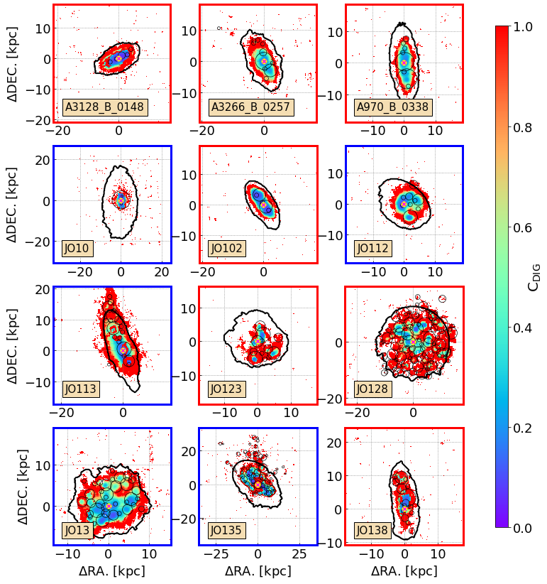
Figure 12: Same as Fig. 5, but for all galaxies. Here, we put panels with control sample with red edges, and stripped galaxies with blue edges, respectively.

Figure 13: Same as Fig. 5, but for all galaxies.

Figure 14: Same as Fig. 5, but for all galaxies.

Figure 15: Same as Fig. 5, but for all galaxies.

Figure 16: Same as Fig. 5, but for all galaxies.

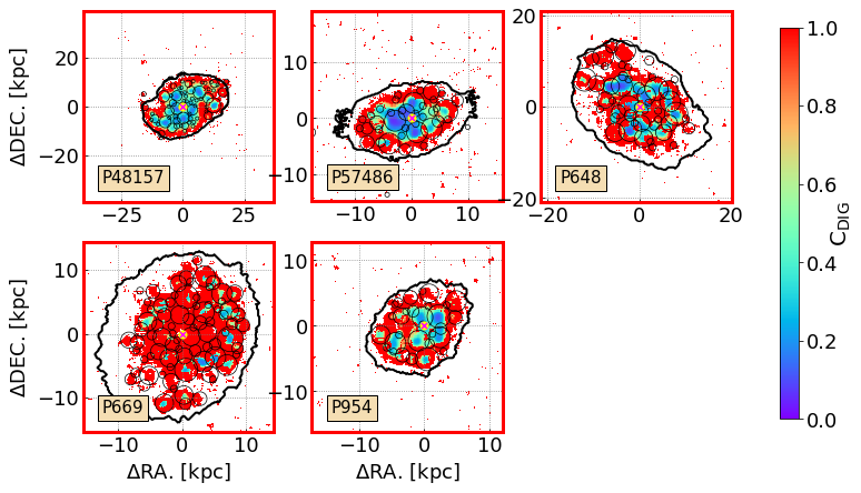
Figure 17: Same as Fig. 5, but for all galaxies.

References

- Astropy Collaboration et al. (2013) Astropy Collaboration, Robitaille, T. P., Tollerud, E. J., et al. 2013, A&A, 558, A33, doi: 10.1051/0004-6361/201322068
- Baldwin et al. (1981) Baldwin, J. A., Phillips, M. M., & Terlevich, R. 1981, PASP, 93, 5, doi: 10.1086/130766
- Barnes et al. (2014) Barnes, J. E., Wood, K., Hill, A. S., & Haffner, L. M. 2014, MNRAS, 440, 3027, doi: 10.1093/mnras/stu521
- Belfiore et al. (2016) Belfiore, F., Maiolino, R., Maraston, C., et al. 2016, MNRAS, 461, 3111, doi: 10.1093/mnras/stw1234
- Bellhouse et al. (2017) Bellhouse, C., Jaffé, Y. L., Hau, G. K. T., et al. 2017, ApJ, 844, 49, doi: 10.3847/1538-4357/aa7875
- Binette et al. (2009) Binette, L., Drissen, L., Ubeda, L., et al. 2009, A&A, 500, 817, doi: 10.1051/0004-6361/200811132
- Blanc et al. (2009) Blanc, G. A., Heiderman, A., Gebhardt, K., Evans, Neal J., I., & Adams, J. 2009, ApJ, 704, 842, doi: 10.1088/0004-637X/704/1/842
- Blanc et al. (2015) Blanc, G. A., Kewley, L., Vogt, F. P. A., & Dopita, M. A. 2015, ApJ, 798, 99, doi: 10.1088/0004-637X/798/2/99
- Bocchio et al. (2016) Bocchio, M., Bianchi, S., Hunt, L. K., & Schneider, R. 2016, A&A, 586, A8, doi: 10.1051/0004-6361/201526950
- Calvi et al. (2011) Calvi, R., Poggianti, B. M., & Vulcani, B. 2011, MNRAS, 416, 727, doi: 10.1111/j.1365-2966.2011.19088.x
- Calzetti et al. (1994) Calzetti, D., Kinney, A. L., & Storchi-Bergmann, T. 1994, ApJ, 429, 582, doi: 10.1086/174346
- Cardelli et al. (1989) Cardelli, J. A., Clayton, G. C., & Mathis, J. S. 1989, ApJ, 345, 245, doi: 10.1086/167900
- Chabrier (2003) Chabrier, G. 2003, PASP, 115, 763, doi: 10.1086/376392
- Cid Fernandes et al. (2011) Cid Fernandes, R., Stasińska, G., Mateus, A., & Vale Asari, N. 2011, MNRAS, 413, 1687, doi: 10.1111/j.1365-2966.2011.18244.x
- Collins & Rand (2001) Collins, J. A., & Rand, R. J. 2001, ApJ, 551, 57, doi: 10.1086/320072
- Della Bruna et al. (2020) Della Bruna, L., Adamo, A., Bik, A., et al. 2020, A&A, 635, A134, doi: 10.1051/0004-6361/201937173
- den Brok et al. (2020) den Brok, M., Carollo, C. M., Erroz-Ferrer, S., et al. 2020, MNRAS, 491, 4089, doi: 10.1093/mnras/stz3184
- Dopita et al. (2013) Dopita, M. A., Sutherland, R. S., Nicholls, D. C., Kewley, L. J., & Vogt, F. P. A. 2013, ApJS, 208, 10, doi: 10.1088/0067-0049/208/1/10
- Draine (2011) Draine, B. T. 2011, Physics of the Interstellar and Intergalactic Medium
- Fasano et al. (2006) Fasano, G., Marmo, C., Varela, J., et al. 2006, A&A, 445, 805, doi: 10.1051/0004-6361:20053816
- Flores-Fajardo et al. (2011a) Flores-Fajardo, N., Morisset, C., Stasińska, G., & Binette, L. 2011a, MNRAS, 415, 2182, doi: 10.1111/j.1365-2966.2011.18848.x
- Flores-Fajardo et al. (2011b) —. 2011b, MNRAS, 415, 2182, doi: 10.1111/j.1365-2966.2011.18848.x
- Fossati et al. (2016) Fossati, M., Fumagalli, M., Boselli, A., et al. 2016, MNRAS, 455, 2028, doi: 10.1093/mnras/stv2400
- Franchetto (in prep.) Franchetto, A. in prep.
- Franchetto et al. (2020) Franchetto, A., Vulcani, B., Poggianti, B. M., et al. 2020, arXiv e-prints, arXiv:2004.11917. https://arxiv.org/abs/2004.11917
- Fritz et al. (2017) Fritz, J., Moretti, A., Gullieuszik, M., et al. 2017, ApJ, 848, 132, doi: 10.3847/1538-4357/aa8f51
- Fumagalli et al. (2014) Fumagalli, M., Fossati, M., Hau, G. K. T., et al. 2014, MNRAS, 445, 4335, doi: 10.1093/mnras/stu2092
- George et al. (2018) George, K., Poggianti, B. M., Gullieuszik, M., et al. 2018, MNRAS, 479, 4126, doi: 10.1093/mnras/sty1452
- Grevesse et al. (1996) Grevesse, N., Noels, A., & Sauval, A. J. 1996, in Astronomical Society of the Pacific Conference Series, Vol. 99, Cosmic Abundances, ed. S. S. Holt & G. Sonneborn, 117
- Gullieuszik et al. (2015) Gullieuszik, M., Poggianti, B., Fasano, G., et al. 2015, A&A, 581, A41, doi: 10.1051/0004-6361/201526061
- Gullieuszik et al. (2020) Gullieuszik, M., Poggianti, B. M., McGee, S. L., et al. 2020, arXiv e-prints, arXiv:2006.16032. https://arxiv.org/abs/2006.16032
- Haffner et al. (2009) Haffner, L. M., Dettmar, R. J., Beckman, J. E., et al. 2009, Reviews of Modern Physics, 81, 969, doi: 10.1103/RevModPhys.81.969
- Heckman & Balick (1980) Heckman, T. M., & Balick, B. 1980, A&A, 83, 100
- Hoopes & Walterbos (2003) Hoopes, C. G., & Walterbos, R. A. M. 2003, ApJ, 586, 902, doi: 10.1086/367954
- Hoopes et al. (1999) Hoopes, C. G., Walterbos, R. A. M., & Rand , R. J. 1999, ApJ, 522, 669, doi: 10.1086/307670
- Jaffé et al. (2018) Jaffé, Y. L., Poggianti, B. M., Moretti, A., et al. 2018, MNRAS, 476, 4753, doi: 10.1093/mnras/sty500
- Kaplan et al. (2016) Kaplan, K. F., Jogee, S., Kewley, L., et al. 2016, MNRAS, 462, 1642, doi: 10.1093/mnras/stw1422
- Kennicutt (1998a) Kennicutt, Robert C., J. 1998a, ARA&A, 36, 189, doi: 10.1146/annurev.astro.36.1.189
- Kennicutt (1998b) —. 1998b, ApJ, 498, 541, doi: 10.1086/305588
- Kreckel et al. (2016) Kreckel, K., Blanc, G. A., Schinnerer, E., et al. 2016, ApJ, 827, 103, doi: 10.3847/0004-637X/827/2/103
- Kreckel et al. (2013) Kreckel, K., Groves, B., Schinnerer, E., et al. 2013, ApJ, 771, 62, doi: 10.1088/0004-637X/771/1/62
- Kumari et al. (2019) Kumari, N., Maiolino, R., Belfiore, F., & Curti, M. 2019, MNRAS, 485, 367, doi: 10.1093/mnras/stz366
- Lacerda et al. (2018) Lacerda, E. A. D., Cid Fernandes, R., Couto, G. S., et al. 2018, MNRAS, 474, 3727, doi: 10.1093/mnras/stx3022
- Madsen et al. (2006) Madsen, G. J., Reynolds, R. J., & Haffner, L. M. 2006, ApJ, 652, 401, doi: 10.1086/508441
- Markwardt (2009) Markwardt, C. B. 2009, in Astronomical Society of the Pacific Conference Series, Vol. 411, Astronomical Data Analysis Software and Systems XVIII, ed. D. A. Bohlender, D. Durand, & P. Dowler, 251. https://arxiv.org/abs/0902.2850
- Mingozzi et al. (2020) Mingozzi, M., Belfiore, F., Cresci, G., et al. 2020, A&A, 636, A42, doi: 10.1051/0004-6361/201937203
- Minter & Balser (1998) Minter, A., & Balser, D. S. 1998, Turbulent Heating in the Galactic Diffuse Ionized Gas, ed. D. Breitschwerdt, M. J. Freyberg, & J. Truemper, Vol. 506, 543–546, doi: 10.1007/BFb0104779
- Minter & Spangler (1997) Minter, A. H., & Spangler, S. R. 1997, ApJ, 485, 182, doi: 10.1086/304396
- Oey et al. (2007) Oey, M. S., Meurer, G. R., Yelda, S., et al. 2007, ApJ, 661, 801, doi: 10.1086/517867
- Osterbrock & Martel (1992) Osterbrock, D. E., & Martel, A. 1992, PASP, 104, 76, doi: 10.1086/132961
- Otte et al. (2002) Otte, B., Gallagher, J. S., I., & Reynolds, R. J. 2002, ApJ, 572, 823, doi: 10.1086/340381
- Poetrodjojo et al. (2019) Poetrodjojo, H., D’Agostino, J. J., Groves, B., et al. 2019, MNRAS, 487, 79, doi: 10.1093/mnras/stz1241
- Poggianti et al. (2017a) Poggianti, B. M., Moretti, A., Gullieuszik, M., et al. 2017a, ApJ, 844, 48, doi: 10.3847/1538-4357/aa78ed
- Poggianti et al. (2017b) Poggianti, B. M., Jaffé, Y. L., Moretti, A., et al. 2017b, Nature, 548, 304, doi: 10.1038/nature23462
- Poggianti et al. (2019a) Poggianti, B. M., Ignesti, A., Gitti, M., et al. 2019a, ApJ, 887, 155, doi: 10.3847/1538-4357/ab5224
- Poggianti et al. (2019b) Poggianti, B. M., Gullieuszik, M., Tonnesen, S., et al. 2019b, MNRAS, 482, 4466, doi: 10.1093/mnras/sty2999
- Raymond (1992) Raymond, J. C. 1992, ApJ, 384, 502, doi: 10.1086/170892
- Reynolds (1984) Reynolds, R. J. 1984, ApJ, 282, 191, doi: 10.1086/162190
- Reynolds & Cox (1992) Reynolds, R. J., & Cox, D. P. 1992, ApJ, 400, L33, doi: 10.1086/186642
- Reynolds et al. (2001) Reynolds, R. J., Sterling, N. C., Haffner, L. M., & Tufte, S. L. 2001, ApJ, 548, L221, doi: 10.1086/319119
- Rueff et al. (2013) Rueff, K. M., Howk, J. C., Pitterle, M., et al. 2013, AJ, 145, 62, doi: 10.1088/0004-6256/145/3/62
- Sanders et al. (2017) Sanders, R. L., Shapley, A. E., Zhang, K., & Yan, R. 2017, ApJ, 850, 136, doi: 10.3847/1538-4357/aa93e4
- Schlafly & Finkbeiner (2011) Schlafly, E. F., & Finkbeiner, D. P. 2011, ApJ, 737, 103, doi: 10.1088/0004-637X/737/2/103
- Schmidt (1959) Schmidt, M. 1959, ApJ, 129, 243, doi: 10.1086/146614
- Slavin et al. (1993) Slavin, J. D., Shull, J. M., & Begelman, M. C. 1993, ApJ, 407, 83, doi: 10.1086/172494
- Stasińska et al. (2008) Stasińska, G., Vale Asari, N., Cid Fernandes, R., et al. 2008, MNRAS, 391, L29, doi: 10.1111/j.1745-3933.2008.00550.x
- Tomičić et al. (2017) Tomičić, N., Kreckel, K., Groves, B., et al. 2017, ApJ, 844, 155, doi: 10.3847/1538-4357/aa7b30
- Tomičić et al. (2019) Tomičić, N., Ho, I. T., Kreckel, K., et al. 2019, ApJ, 873, 3, doi: 10.3847/1538-4357/ab03ce
- Vale Asari et al. (2019) Vale Asari, N., Couto, G. S., Cid Fernandes, R., et al. 2019, MNRAS, 489, 4721, doi: 10.1093/mnras/stz2470
- Vale Asari & Stasińska (2020) Vale Asari, N., & Stasińska, G. 2020, arXiv e-prints, arXiv:2005.06054. https://arxiv.org/abs/2005.06054
- Vale Asari et al. (2020) Vale Asari, N., Wild, V., de Amorim, A. L., et al. 2020, arXiv e-prints, arXiv:2007.05544. https://arxiv.org/abs/2007.05544
- Vandenbroucke & Wood (2019) Vandenbroucke, B., & Wood, K. 2019, MNRAS, 488, 1977, doi: 10.1093/mnras/stz1841
- Vogt et al. (2015) Vogt, F. P. A., Dopita, M. A., Borthakur, S., et al. 2015, MNRAS, 450, 2593, doi: 10.1093/mnras/stv749
- Vulcani et al. (2018) Vulcani, B., Poggianti, B. M., Moretti, A., et al. 2018, ApJ, 852, 94, doi: 10.3847/1538-4357/aa992c
- Vulcani et al. (2019a) —. 2019a, MNRAS, 488, 1597, doi: 10.1093/mnras/stz1829
- Vulcani et al. (2019b) —. 2019b, MNRAS, 487, 2278, doi: 10.1093/mnras/stz1399
- Vulcani et al. (2020) Vulcani, B., Poggianti, B. M., Tonnesen, S., et al. 2020, arXiv e-prints, arXiv:2007.04996. https://arxiv.org/abs/2007.04996
- Walterbos & Braun (1994) Walterbos, R. A. M., & Braun, R. 1994, ApJ, 431, 156, doi: 10.1086/174475
- Weingartner & Draine (2001) Weingartner, J. C., & Draine, B. T. 2001, ApJS, 134, 263, doi: 10.1086/320852
- Zhang et al. (2017) Zhang, K., Yan, R., Bundy, K., et al. 2017, MNRAS, 466, 3217, doi: 10.1093/mnras/stw3308