Lensed CMB power spectrum biases from masking extragalactic sources

Abstract

The cosmic microwave background (CMB) is gravitationally lensed by large-scale structure, which distorts observations of the primordial anisotropies in any given direction. Averaged over the sky, this important effect is routinely modelled with the lensed CMB power spectra. This accounts for the variance of this distortion, where the leading variance effect is quadratic in the lensing deflections. However, we show that if bright extragalactic sources correlated with the large-scale structure are masked in a CMB map, the power spectrum measured over the unmasked area using a standard pseudo-$C_{\ell}$ estimator has an additional linear lensing effect arising from correlations between the masked area and the lensing. This induces a scale-dependent average demagnification of the unlensed distance between unmasked pairs of observed points and a negative contribution to the CMB correlation function peaking at $\sim 10\,{\rm arcmin}$. We give simple analytic models for point sources and a threshold mask constructed on a correlated Gaussian foreground field. We demonstrate the consistency of their predictions for masks removing radio sources and peaks of Sunyaev-Zeldovich and cosmic infrared background emissions using realistic numerical simulations. We discuss simple diagnostics that can be used to test for the effect in the absence of a good model for the masked sources and show that by constructing specific masks the effect can be observed on Planck data. For masks employed in the analysis of Planck and other current data sets, the effect is likely to be negligible, but may become an important subpercent correction for future surveys if substantial populations of resolved sources are masked.

I Introduction

CMB observations are inevitably contaminated at some level by foregrounds, from galactic dust and synchrotron emission to a range of extragalactic signals including the cosmic infrared background (CIB), thermal Sunyaev-Zeldovich effect (tSZ), and radio point sources. These extragalactic signals are correlated to the matter density at the foreground source redshifts, and point source brightness may also be affected by line-of-sight gravitational lensing. Much of the foreground signal can either be modelled or removed using the distinct frequency dependence. However, bright sources can be problematic and are often masked out. It is usually tacitly assumed that the CMB power spectra estimated over the unmasked areas are then unbiased estimates that can be used to study cosmology. As long as sources with strong correlation to lensing are not masked, for current data this is likely to be a safe approximation. For future data, where large populations of extragalactic sources will be resolved, corrections may become important. We quantify the likely size of the bias due to mask correlations, as well as proposing empirical consistency tests than can be used in the absence of detailed models or predictions for the source populations.

The CMB is lensed by the large-scale structure along the line of sight, and hence some correlation between extragalactic sources and the CMB lensing convergence is inevitable. The effect of CMB lensing on the full-sky CMB power spectra is well understood and routinely modelled Seljak (1996); Challinor and Lewis (2005): the varying magnification and shear of the unlensed acoustic peaks as a function of position on the sky leads to a small smoothing of the peaks in the power spectrum, and the small-scale lenses also increase the power in the CMB damping tail. These are both effects quadratic in the lensing, since over the full sky the convergence and shear average to zero. However, if bright extragalactic sources are masked, due to the correlation of the source density with the lensing this will preferentially be removing peaks of the CMB lensing convergence. If the power spectrum is now estimated only using the unmasked area, there can be additional net effect that is linear in the lensing. The correlation between the deflection angle around convergence peaks is relatively long range, peaking at around $20\,{\rm arcmin}$, so every masked peak is associated with a surrounding area of correlated deflection angle that distorts (magnifies) the unlensed CMB. When these peaks are masked, the corresponding regions of demagnifying deflection angle are no longer fully balanced, and the net effect is a scale-dependent net average demagnification.

The effect of a constant demagnification on the CMB is easily understood: it simply shifts angular scales so that everything looks smaller and the CMB power spectrum is therefore shifted toward higher harmonic multipole $\ell$. At any given observed $\ell$, the CMB power is then the same as at a lower pre-demagnification $\ell$, which on small scales is larger because the CMB power decreases rapidly with $\ell$, leading to an increase in power on small scales (and a corresponding decrease on large scales). Since the angular acoustic scale is shifted to smaller values, corresponding to the acoustic peaks being shifted to smaller scales, and there is also a strongly oscillatory difference between the power spectra. Due to the steep fall of the CMB spectrum with $\ell$ in the damping tail, a small constant demagnification can lead to non-negligible signatures on the power spectrum. Plausible numbers may be given as follows: removing $2\%$ of the sky on the convergence peaks would give a mean convergence $\langle\kappa\rangle\approx-0.003$ over the remaining unmasked area. This leads to a significant $1\%$ change in the temperature spectrum at $\ell\sim 2000$, and larger on smaller scales. This crude estimate is one motivation to the more careful analysis that we give in this paper. For future data, with the CMB power spectrum measured to nearly cosmic variance out to small scales, any small percent-level corrections would have to be carefully accounted for.

In this constant demagnification picture, the effect would be almost degenerate with a change in the angular diameter distance to the CMB (the effect from large-scale lenses would be like a mask-correlated lensing super-sample variance Manzotti et al. (2014)). However, this model is not accurate, since the effective net demagnification is both mode-orientation and scale dependent. The degree-scale acoustic features are only slightly affected because the deflection-convergence correlation peaks on smaller scales, about $20\,{\rm arcmin}$. The corresponding effect on the power spectrum is therefore distinctive, and important corrections actually arise mostly from relatively smaller-scale lenses.

We start in Sec. II by giving a simple leading-order analytic model for the effect in terms of a general mask-deflection correlation function. We give specific analytic forms for the case of masking the most relevant CMB extragalactic foreground emission correlated with CMB lensing: Poisson point sources (an approximate model for radio sources), and peaks above some threshold in a Gaussian isotropic convergence or foreground field (a model for tSZ sources and a component of the infrared sources). We show that this model is sufficient to accurately calculate the effect when these assumptions hold, leaving details of a fully nonperturbative calculation to Appendix B.

In Sec. III we test the models and compare analytic predictions with results based on realistic numerical simulations which include non-Gaussian correlated maps of the CMB lensing convergence, tSZ and CIB emission at various frequencies as well as radio sources. In real-world analyses, masks are usually apodized to remove ringing effects when estimating power spectra in harmonic space. Although this case is harder to model fully analytically, we show that semianalytic estimates of the bias based on the mask-lensing correlation measured in the simulated maps describes the bias measured in simulations quite accurately.

In this paper, we focus on the effect of masking on the CMB power spectra. In a companion paper Lembo et al. we consider the impact on lensing reconstruction, for which the preliminary investigation of Refs. Harnois-Déraps et al. (2016); Liu and Hill (2015) suggested a similar effect might be important in particular for cross-correlation between CMB lensing and external matter tracers. Since extragalactic foregrounds are most dominant for the small-scale CMB temperature we focus on that, however some bright extragalactic polarized sources may also have to be masked, so the impact on polarization is also potentially important Lagache et al. (2020). We include a few numerical and analytic results for polarization for completeness, but leave a more detailed quantitative analysis of the likely impact of masking polarized sources to future work (the effect would be both experiment and spectrum estimator dependent).

II Modelling

The effects of masking are largely on small scales, so for simplicity we use the flat-sky approximation in the main text, where the lensed temperature $\tilde{T}(\bm{x})=T(\bm{x}+{\bm{\alpha}}(\bm{x}))$ is related to the unlensed temperature $T$ via the lensing deflection angle ${\bm{\alpha}}(\bm{x})$. In Appendix B.1 we also provide leading-order curved-sky results .

It is convenient to work mostly in position space using a correlation function approach, just as for the usual lensed CMB spectra Challinor and Lewis (2005). The lensed correlation function is defined by

$$\tilde{\xi}(r)\equiv\langle\tilde{T}(\bm{x})\tilde{T}(\bm{x}+\bm{r})\rangle,$$ (1)

and is independent of $\bm{x}$ and the direction of $\bm{r}$ for a homogeneous statistically isotropic field. From a statistically isotropic map with a fixed mask an estimator for the lensed CMB correlation function can be built by spatial averaging. In the absence of noise and assuming all distances $r$ can be probed at least once, an estimator is Szapudi et al. (2001); Chon et al. (2004)

$$\hat{\tilde{\xi}}(r)\equiv\frac{\left\langle({W}\tilde{T})(\bm{x})({W}\tilde{T})(\bm{x}+\bm{r})\right\rangle_{\bm{x},\phi_{r}}}{{\left\langle{W}(\bm{x}){W}(\bm{x}+\bm{r})\right\rangle}_{\bm{x},\phi_{r}}}.$$ (2)

The normalization in the denominator is required for the estimator to be unbiased in the case where the lensed temperature distribution is independent of the mask. After transforming to the power spectrum, the correlation function estimator is equivalent to a standard “pseudo-$C_{\ell}$” estimator with mask ${W}(\bm{x})$ Wandelt et al. (2001). In the presence of mask-lensing correlations, this estimator is no longer unbiased, since the conditional distribution for the lensed temperature given the fixed mask is no longer statistically isotropic. This is the bias we aim to quantify.

The mask ${W}(\bm{x})$ is a function of position on the sky, which is zero over sources that are masked out. For an extragalactic source mask, where ${W}(\bm{x})$ is constructed based on the realization of statistically isotropic sources, ${W}(\bm{x})$ can also be viewed as a statistically isotropic random field. The denominator in Eq. (2) is its empirical two-point correlation function, which we denote ${\hat{\xi}_{\rm mask}}(r)$. With $f_{\rm sky}$ the average of the mask across the sky, ${\hat{\xi}_{\rm mask}}(r)$ is a smooth function varying from $f_{\rm sky}^{2}$ at separations larger than all relevant correlation lengths, to $f_{\rm sky}$ for separations much smaller than the typical mask hole size where both points are almost surely both inside or both outside the mask.

We now turn to the calculation of the expectation values and biases entering the estimator given by Eq. (2). We proceed by replacing spatial averages with expectations values over ensembles of $T,W$ at fixed $\bm{x}$ and $\bm{r}$. Since we model the mask as a random field, there is a slight possible ambiguity in this approach. In practice, for simulating CMB data, both CMB and extragalactic foreground skies should be varied at the same time. With the extragalactic part of mask varying with the foregrounds, the CMB correlations must be deconvolved from the mask realization per realization: the estimator mean is the expectation value of the ratio in Eq. (2), rather than the ratio of expectation values. However, we show in Appendix A that these are equivalent for binary masks.

The numerator of Eq. (2) becomes simply the un-normalized pseudocorrelation function of the masked temperature

$$\tilde{\xi}_{\rm masked}(r) \equiv\left\langle({W}\tilde{T})(\bm{x})({W}\tilde{T})(\bm{x}+\bm{r})\right\rangle$$

$$=\left\langle T(\bm{x}+{\bm{\alpha}}(\bm{x}))T(\bm{x}^{\prime}+{\bm{\alpha}}(\bm{x}^{\prime})){W}(\bm{x}){W}(\bm{x}^{\prime})\right\rangle,$$ (3)

where $\bm{x}^{\prime}=\bm{x}+\bm{r}$. Expanding into flat-sky harmonics and taking the unlensed CMB $T$ to be uncorrelated to anything else, we then have

$$\tilde{\xi}_{\rm masked}(r)=\int\frac{{\rm d}^{2}\bm{l}}{(2\pi)^{2}}C_{l}e^{i\bm{l}\cdot\bm{r}}\left\langle e^{i\bm{l}\cdot({\bm{\alpha}}(\bm{x})-{\bm{\alpha}}(\bm{x}^{\prime}))}{W}(\bm{x}){W}(\bm{x}^{\prime})\right\rangle.$$ (4)

In this equation $C_{l}$ is the unlensed temperature power spectrum. The leading correction in $\alpha$ to the masked correlation function from mask correlations is then

$$\Delta\tilde{\xi}_{\rm masked}(r)\equiv\tilde{\xi}_{\rm masked}(r)-\tilde{\xi}(r){\xi_{\rm mask}}(r)$$ (5)

$$\approx\int\frac{{\rm d}^{2}\bm{l}}{(2\pi)^{2}}C_{l}e^{i\bm{l}\cdot\bm{r}}\left\langle i\bm{l}\cdot({\bm{\alpha}}(\bm{x})-{\bm{\alpha}}(\bm{x}^{\prime})){W}(\bm{x}){W}(\bm{x}^{\prime})\right\rangle$$

$$=\partial_{r}\xi(r)\left\langle(\alpha_{r}(\bm{x})-\alpha_{r}(\bm{x}^{\prime})){W}(\bm{x}){W}(\bm{x}^{\prime})\right\rangle.$$ (6)

In the last line we introduced $\alpha_{r}$, the components of the deflection parallel to $\bm{r}$ at $\bm{x}$ and $\bm{x}^{\prime}$, and the unlensed CMB correlation function $\xi(r)$. The result for the polarization correlation functions has exactly the same form, with $\xi$ replaced by $\xi_{+}$ or $\xi_{-}$ for polarization or $\xi_{\times}$ for the temperature cross-correlation. At lowest order, the unlensed correlation function $\xi(r)$ can equally well be replaced by the standard lensed correlation function $\tilde{\xi}(r)$, which leads to a better approximation as it captures the main nonperturbative standard lensing effects (see Appendix B for a more accurate result). The expectation in Eq. (6) is just the average difference between the lensed and unlensed distance between any two points (allowing for masking this is positive), and the derivative term then gives how much the correlation function changes due to the mean shift in separation (negative since the correlation falls with distance on relevant scales).

Dividing by ${\xi_{\rm mask}}(r)$, the normalized (mask-deconvolved) correction to the correlation function is therefore always of the product form

$$\Delta\tilde{\xi}\approx\partial_{r}\tilde{\xi}(r)\bar{\Delta}(r),$$ (7)

where from Eq. (6) we defined $\bar{\Delta}(r)$ as the average over the unmasked area of change in the separation of points due to lensing

$$\bar{\Delta}(r)\equiv \frac{\langle[\alpha_{r}(\bm{x})-\alpha_{r}(\bm{x}^{\prime})]{W}(\bm{x}){W}(\bm{x}^{\prime})\rangle}{\langle{W}(\bm{x}){W}(\bm{x}^{\prime})\rangle}$$ (8)

$$= 2\frac{\langle\alpha_{r}(\bm{x}){W}(\bm{x}){W}(\bm{x}^{\prime})\rangle}{\langle{W}(\bm{x}){W}(\bm{x}^{\prime})\rangle},$$ (9)

where in the last equation we used the symmetry properties of $\langle\alpha_{r}(\bm{x}){W}(\bm{x}){W}(\bm{x}^{\prime})\rangle$ under the coordinates transformation $\bm{x}\rightarrow\bm{x}^{\prime}$ (see Sec. II.2). The unmasked area can therefore be thought of as having scale-dependent demagnification of the distance between points, with $\tilde{\xi}(r)|_{\textrm{unmasked area}}\sim\tilde{\xi}(r+\bar{\Delta}(r))$. The product form of Eq. (7) in real space corresponds in harmonic space to a convolution of the CMB temperature-gradient power with the power spectrum corresponding to $\bar{\Delta}$.

In Sec. II.1 we first give a recipe to estimate the bias in Eq. (7) from simulations. We then proceed with analytic methods in Sec. II.2. There we start by discussing results for masks built locally from some Gaussian foreground field $f$. We then look in more detail at two mask models: in Sec. II.2.1 we discuss thresholding the peaks of $f$, where the effect can be significant, then in Sec. II.2.2 we consider masking sources that are modelled as a Poisson sampling of $f$, as a model of masking radio point source (where the effect is typically much smaller). A set of appendices collect details of the calculations related to these two models.

II.1 Empirical estimation of the bias

Equation (9) can in principle be calculated empirically for any mask construction if the required average can be calculated from simulations that capture the relevant correlations and (potentially non-Gaussian) statistics. The quantity $\langle\alpha_{r}(\bm{x}){W}(\bm{x}){W}(\bm{x}^{\prime})\rangle$ appearing in Eq. (9) is just the correlation function of the gradient mode of the masked deflection angle with the mask. For any given simulation, where we know ${W}$ and $\kappa$ (and hence the deflection ${\bm{\alpha}}$), we can estimate $\bar{\Delta}(r)$ directly from the cross-spectrum between the masked deflection and the mask measured in that simulation.

More explicitly, if $E(\bm{l})$ and $B(\bm{l})$ are the gradient and curl modes of the spin-1 field $\alpha{W}$, and ${W}(\bm{l})$ the Fourier coefficients of the spin-0 mask, we may write on the flat-sky

$$\hat{\bm{r}}\cdot{\bm{\alpha}}W=\int\frac{{\rm d}^{2}\bm{l}}{2\pi}\left(E(\bm{l})\hat{\bm{r}}\cdot\hat{\bm{l}}+B(\bm{l})\hat{\bm{r}}\star\hat{\bm{l}}\right)ie^{i\bm{l}\cdot\bm{x}}$$ (10)

with $\hat{\bm{r}}\star\hat{\bm{l}}=\hat{\bm{r}}\cdot(-\sin\phi,\cos\phi)$. Correlating with $W(\bm{x}^{\prime})$ gives

$$\langle\alpha_{r}(\bm{x}){W}(\bm{x}){W}(\bm{x}^{\prime})\rangle=-\int\frac{{\rm d}l}{2\pi}lC_{l}^{EW}J_{1}(lr).$$ (11)

The denominator in Eq. (9) can also be calculated directly from the mask power spectrum with a spin-0 (here, $J_{0}$) transform.

The leading correction to the correlation function can therefore easily be evaluated from corresponding power spectra. For any masking recipe, this therefore provides a straightforward way to calculate the expected bias in the power spectrum measured over the unmasked area. On data, the deflection field is not known, but it may be possible to estimate it, at least crudely, from a correlated field (e.g. the CIB) or lensing reconstruction, providing an internal estimate of the expected bias without having a detailed model for the statistics of the mask.

II.2 Analytic models

For a first analytic model, we assume that some underlying Gaussian statistically-isotropic foreground field $f(\bm{x})$ determines the mask probability locally, so that ${W}(\bm{x})$ only depends on some (in general nonlinear) function of $f(\bm{x})$. We will consider two specific analytic models for the mask construction, a peak threshold mask (where the effect can be substantial) and Poisson sources (where the effect is generally small). When considering a threshold mask we will consider specifically the case where $f$ is tSZ or CIB fields, or as an extreme limiting case, the CMB lensing convergence $\kappa$ itself. For Poisson sources, $f$ will be the perturbation to the expected number of sources over the area masked out per source, determined by the perturbations to the underlying galaxy populations, which we approximate as Gaussian.

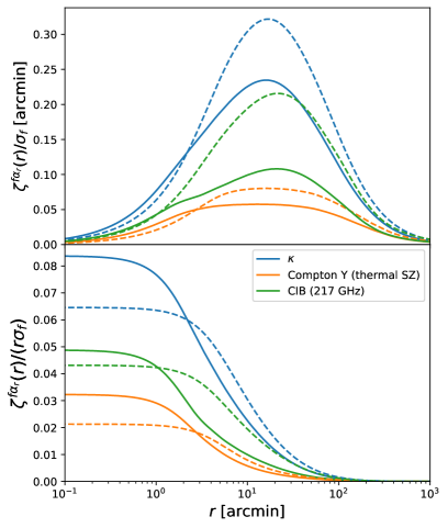
Figure 1: The correlation between the size of the (inward pointing) radial lensing deflection about a point and the deviation of the field $f$ at that point from its mean in units of the standard deviation: for a point with a foreground field that is $1\sigma_{f}$ above the mean, the plots show the mean inward-pointing radial lensing deflection at radius $r$. The top plot shows the result in arcminutes, the bottom shows the fractional change in distance between the points due to the deflection. Different colours correspond to the limiting case of a field that is fully correlated, $f\propto\kappa$ (blue), and the result expected for Compton Y (thermal SZ foreground, orange) or cosmic infrared background foreground at 217 Ghz (green). The latter results are based on a smooth fit to the Websky simulation power spectra Stein et al. (2020). Solid lines are for the field values after smoothing with a 1.7 FWHM beam, dashed the corresponding result for a 5.1 FWHM beam. The correlation extends to cosmologically important distances, and the fractional change in radius becomes percent level on scales below 10s of arcminutes.

By symmetry, at a point there is no correlation between the scalar foreground $f$ and the vector deflection angle, $\langle f(\bm{x}){\bm{\alpha}}(\bm{x})\rangle=0$. However, if $f$ is correlated to large-scale structure it will be correlated to the lensing convergence, and hence have a nonzero correlation $\xi^{f\alpha_{i}}(\bm{r})\equiv\langle f(\bm{x})\alpha_{i}(\bm{x}^{\prime})\rangle=-\langle\alpha_{i}(\bm{x})f(\bm{x}^{\prime})\rangle\equiv\xi^{f\alpha_{r}}\hat{r}_{i}$, corresponding e.g. to deflection angles around overdensities having an inward-pointing radial direction (positive $\xi^{\kappa\alpha_{r}}$ for our definition of $\bm{r}\equiv\bm{x}^{\prime}-\bm{x}$ and $\kappa=-\nabla\cdot{\bm{\alpha}}/2$). If $\phi$ is the lensing potential with ${\bm{\alpha}}=\nabla\phi$, then its explicit form is

$$\xi^{f\alpha_{r}}(r)=-\partial_{r}\xi^{f\phi}(r)=\int\frac{{\rm d}l}{2\pi}\>l^{2}C^{f\phi}_{l}J_{1}(lr).$$ (12)

As shown in Fig. 1, $\xi^{f\alpha_{r}}(r)$ peaks somewhere around $r\sim 20\,{\rm arcmin}$ depending on the field being considered.

Since we are only considering the two-point CMB correlation function, for any choice of coordinates the correlation function is an average over the correlated Gaussian variables $f(\bm{x}),f(\bm{x}^{\prime}),{\bm{\alpha}}(\bm{x})-{\bm{\alpha}}(\bm{x}^{\prime})$. The expectations in Eq. (6) can then be evaluated for Gaussian fields to give

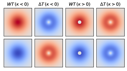
Figure 2: An illustration of the lensing effect on a temperature hot spot (top row) or cold spot (bottom row). The columns show the unlensed temperature and change in temperature due to lensing by the expected radial deflection if there is a convergence minimum (left two columns) or peak (right two columns) in the centre. The unlensed temperature and lensing colour scales are not the same to make the much smaller lensing signal easily visible. The temperature $T$ in the centre is unchanged by an aligned lens, and is positively correlated with the ring of lensing signal $\Delta T$ if the lensing is converging ($\kappa>0$), and negatively correlated if the lens is diverging ($\kappa<0)$. For Gaussian fields both signs are equally common, and the correlation averages to zero when there is no masking. If the centre of the lens is preferentially removed by a mask $W$ when $\kappa>0$ due to correlation between foregrounds and the convergence, there will be more points of negative correlation between the centre and the ring, giving a net negative change to the lensed CMB correlation function at radius $r>0$. In harmonic space, masking of the temperature at a convergence peak leads to net negative correlation between the large-scale temperature and lensing correction, leading to a negative contribution to the large-scale pseudo power spectrum. On small scales (but larger than the hole size), there is a ring-like pattern in both the masked temperature and lensing signal at a convergence peak, hence there is a positive correlation between them leading to an enhancement of small-scale pseudo power spectrum (which is not removed by a mask deconvolution that does not account for the mask correlation). Since the lensing signal is much smaller than the unlensed temperature, the cross-correlation terms dominate the effect on the power spectrum compared to small changes due to also masking the lensing signal.

$$\Delta\tilde{\xi}(r)\approx g(r)\partial_{r}\tilde{\xi}(r)\frac{\xi^{f\alpha_{r}}(r)}{\sigma_{f}},$$ (13)

where

$$g(r)\equiv-\frac{2\sigma_{f}\bar{f}(r)}{\sigma_{f}^{2}+\xi_{f}(r)},\quad\bar{f}(r)\equiv\frac{\left\langle f(\bm{x}){W}(\bm{x}){W}(\bm{x}^{\prime})\right\rangle}{\left\langle{W}(\bm{x}){W}(\bm{x}^{\prime})\right\rangle}.$$ (14)

Here $\bar{f}(r)$ is the mean of the foreground field over the unmasked area weighted by the number of pairs of points each point forms with separation $r$, which is usually negative. In Eq. (13), $g(r)$ is a very smooth prefactor which, in all models we considered, varies by a factor of two across all distances. For separations large compared to the correlation length ($\xi_{f}(r)\ll\sigma_{f}^{2}$) and hole size, the foreground mean becomes the simple mean over the unmasked area, $\bar{f}(r)\rightarrow\bar{f}$, hence for large separations we have

$$\Delta\tilde{\xi}(r)\approx-2\partial_{r}\tilde{\xi}(r)\frac{\bar{f}}{\sigma_{f}}\frac{\xi^{f\alpha_{r}}(r)}{\sigma_{f}}.$$ (15)

For very small separations, assuming the mask holes have finite size so the two points are almost surely either inside the same hole or both unmasked, ${W}(\bm{x}^{\prime})\approx{W}(\bm{x})={W}(\bm{x})^{2}$ and $\xi_{f}(r)\approx\sigma_{f}^{2}$ so that

$$\Delta\tilde{\xi}(r)\approx-\partial_{r}\tilde{\xi}(r)\frac{\bar{f}}{\sigma_{f}}\frac{\xi^{f\alpha_{r}}(r)}{\sigma_{f}}.$$ (16)

The $\frac{\bar{f}}{\sigma_{f}}\frac{\xi^{f\alpha_{r}}(r)}{\sigma_{f}}$ term is simply the mean radial deflection at one of a pair of points separated by $r$ over the unmasked area. For large separations, where the foreground values at the points are uncorrelated, the total relative change in separation of the two points is twice this. Equations (15) and (16) are of the form of the product of two real space functions. In harmonic space, the result is therefore a convolution, so on large scales compared to the foreground correlation length and hole size the correction to the power spectrum is

$$\Delta\tilde{C}_{l}\sim-2\frac{\bar{f}}{\sigma_{f}^{2}}\int\frac{{\rm d}^{2}\bm{l}^{\prime}}{(2\pi)^{2}}\tilde{C}_{l^{\prime}}C^{\phi f}_{|\bm{l}-\bm{l}^{\prime}|}\bm{l}^{\prime}\cdot(\bm{l}-\bm{l}^{\prime}),$$ (17)

where $C^{\phi f}_{l^{\prime}}$ is the cross-spectrum between the lensing potential and the foreground. For a foreground that scales roughly like the convergence, the convolution is with a kernel that goes like the $\alpha\kappa$ spectrum, which has more small-scale power compared to the $\alpha\alpha$ spectrum that enters the convolution for the leading-order standard lensing effect. This leads to much broader mixing of scales, giving a relatively non-peaky result mixing contributions from different acoustic peaks, and efficiently transfers power to small scales where the CMB spectrum is small. If we consider an $l$ in the damping tail (i.e. much higher than the peak of the temperature gradient spectrum at $l\sim 1000$), where the power spectrum is small, most of the integrand comes from $l^{\prime}\ll l$; in this limit, the leading term is

$$\Delta\left(l^{2}\tilde{C}_{l}\right)\sim 2\frac{\bar{f}}{\sigma_{f}^{2}}\frac{{\rm d}C_{l}^{\kappa f}}{d\ln l}\int\frac{{\rm d}l^{\prime}}{l^{\prime}}\frac{{l^{\prime}}^{4}\tilde{C}_{l^{\prime}}}{2\pi}.$$ (18)

Since $\bar{f}$ is negative when masking peaks, the result is positive when $C_{l}^{\kappa f}$ is decreasing at high $l$ where the limit applies. It vanishes only when there is no foreground-lensing correlation or a cross-correlation spectrum $C_{l}^{\kappa f}$ that is constant (white, which corresponds to no spatial correlation between the foreground value and surrounding lensing field). The integral over the CMB spectrum quantifies the total power from larger scales in the correlation between the CMB temperature and its curvature. The correction spectrum falls much less quickly than the unlensed CMB, and when there are substantial correlations can become a large fractional correction deep in the damping tail; in the high $l$ limit it can become comparable to the standard lensing signal, which is given in this limit by

$$l^{2}\tilde{C}_{l}\sim 2C_{l}^{\kappa}\int\frac{{\rm d}l^{\prime}}{l^{\prime}}\frac{{l^{\prime}}^{4}\tilde{C}_{l^{\prime}}}{2\pi}.$$ (19)

See Fig. 2 for an illustration of the effect on the lensed CMB signal in real space when masking convergence peaks and Fig. 3 for its harmonic domain version.

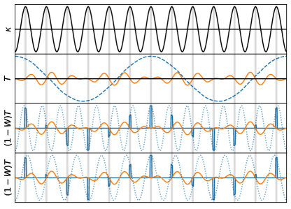
Figure 3: An illustration of the lensing effect of a small-wavelength convergence plane wave $\kappa$ (top panel) on an aligned longer-wavelength CMB temperature modes (second panel, dashed line). Remapping points with the corresponding deflection angles gives the lensing correction (solid orange, greatly exaggerated in relative size for illustration). The vertical bands show the peaks of the convergence, which are preferentially masked if a masked foreground is correlated to the lensing. The third and bottom panels show the temperature values that are removed by masking the peaks of the convergence to calculate a pseudo power spectrum (solid blue lines). Dotted lines show a Fourier component of these values (at the sum and difference of the lens and CMB frequencies respectively). The higher-frequency component in the third panel is negatively correlated with the lensing signal oscillations shown in orange; the lower-frequency component in the bottom panel is positively correlated with the lensing. Since the temperature is much larger than the lensing signal, the cross-correlation can be similar or larger than the lensing auto spectrum even if only a small area at the peaks is masked. On small scales the temperature and lensing spectrum fall with $l$, so more negative cross-correlation is removed by masking than positive is added, leading to a net positive signal that is linear in the lensing. This also leads to a positive bias on the power spectrum estimator after deconvolving the pseudospectrum assuming statistical isotropy over the unmasked area.

II.2.1 Peaks of foreground fields

For a mask that is constructed by thresholding the foreground to mask out the peaks, i.e. a step function ${W}(\bm{x})=\Theta(\nu\sigma_{f}-f(\bm{x}))$ where $\nu$ determines the “sigma” value of the cut, the derivative of ${W}(\bm{x})$ is just a delta function. The remaining Gaussian integral over $f(\bm{x})$ to calculate the expectation in Eq. (14) can then be done to give

$$g(r){\xi_{\rm mask}}(r)=\frac{e^{-\nu^{2}/2}}{\sqrt{2\pi}}\left[1+\textrm{erf}\left(\frac{\nu}{\sqrt{2}}\sqrt{\frac{\sigma_{f}^{2}-\xi_{f}(r)}{\sigma_{f}^{2}+\xi_{f}(r)}}\right)\right].$$ (20)

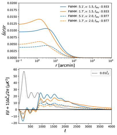
Figure 4: Top: the average fractional change in the separation $r$ of pairs of points in the unmasked area as a function of separation for a thresholded foreground field [see Eq. (9)]. This is assuming an unapodized mask is constructed by thresholding $\nu\sigma$ of a Gaussian foreground field proportional to the lensing convergence after Gaussian smoothing with the given beam full-width-half-maximum (FWHM). Below the acoustic scale, the effect becomes percent-level, and is relatively more important in the power spectrum due to the rapid fall in power on Silk-damping scales. Bottom: the corresponding correction to the lensed CMB temperature power spectrum $\tilde{C}_{l}$ estimated from the unmasked area (the dotted line shows the one hundredth of the full power spectrum for comparison). Results for SZ and CIB-thresholded maps have similar shapes but with lower amplitude proportional to their lower lensing correlation.

The normalization ${\xi_{\rm mask}}(r)$ generally needs to be calculated numerically, but varies between $\sim f_{\rm sky}^{2}$ at large $r$ where the foreground fields are nearly uncorrelated, to $\sim f_{\rm sky}$ for small $r$ where both points are almost surely either both inside or outside the mask. The transition between these values is very smooth and determined by the correlation length of the foreground field. The expected observed sky fraction is

$$\langle f_{\rm sky}\rangle=\langle{W}(\bm{x})\rangle=\frac{1}{2}\left[1+\text{erf}(\nu/\sqrt{2})\right].$$ (21)

The factor in the square brackets in Eq. (20) varies smoothly between $\sim 2f_{\rm sky}$ when $\xi_{f}(r)\ll\sigma_{f}^{2}$ (for $r$ much larger than the correlation length) to unity on very small scales. The factor $-e^{-\nu^{2}/2}/\sqrt{2\pi}=\langle f{W}\rangle/\sigma_{f}=f_{\rm sky}\bar{f}/\sigma_{f}$ is the mean masked value of $f$ in units of its standard deviation, which is negative, where (as before) $\bar{f}$ as the mean value of $f$ over the unmasked area. It therefore has the general limiting forms given for large $r$ by Eq. (15) and small $r$ by Eq. (16). Note that the result is independent of the scale or normalization of $f$, so the effect is leading order in the perturbations (linear in $\alpha_{r}$), and will only be negligible when the correlation is very low or $f$ is dominated by very small scales so that $\bar{f}/\sigma_{f}$ is small.

Although the mean deflection at any distance is very small, less than a quarter of an arcminute, the mean relative change in distance $\bar{\Delta}(r)/r$ is an important percent-level effect at scales of tens of arcminutes and below when masking foreground peaks; see Fig. 4. A typical full numerical result for the correlation function correction over the unmasked area, $\Delta\tilde{\xi}(r)$, is shown in Fig. 5 for a smoothed foreground $f\propto\kappa$ that is threshold-masked with $\nu=2$. The signal peaks at around $10\,{\rm arcmin}$; on much smaller scales the CMB is very smooth so $\partial_{r}\tilde{\xi}(r)\rightarrow 0$, and on much larger scales the deflections have little correlation and only a small fractional effect.

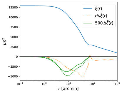
Figure 5: The lensed CMB correlation function $\tilde{\xi}(r)$ (blue solid), and its log derivative (dotted orange). The green lines show the correction $\Delta\tilde{\xi}(r)$ due to threshold masking of a fully-correlated foreground with $f\propto\kappa$ smoothed with a $1.7$ (solid) or $5.1$ (dashed) ${\rm arcmin}$ FWHM Gaussian beam with a $\nu=2$ threshold mask ($f_{\rm sky}\approx 0.977$). In the power spectrum the effect is a much larger fractional correction on small scales, since it adds power on scales where the lensed correlation function has little; on large scales the negative sign of the correction corresponds to a small reduction in power at $l\lesssim 1000$.

If $f$ is band limited or smoothed to a certain scale, so that $C_{l}^{\phi f}$ starts to fall off sharply with $l$, the signal will also decline at the same scale, and the approximation limit will no longer be valid. The full shape of $\bar{\Delta}(r)/r$ shown in Fig. 4 has a peak in between the small and large-scale limits, determined by the clustering scale of the foreground that determines the size of the mask holes. As scales transition from the large-scale to small-scale limit, this translates into a change in sign of the second derivative, $\partial_{r}^{2}\Delta\tilde{\xi}(r)$. For the power spectrum, this corresponds to the correction going negative at high $l$ (for high $l$, the integral of $J_{0}(lr)$ against a smooth function depends on the second derivatives because the fast oscillations average to zero for constant and constant gradient terms).

It may seem quite unintuitive that an effect being sourced from a small sky-fraction mask could be a large fractional effect on the total: doesn’t this imply that at each masked point the effect must be very large? From Fig. 1, for a 1-sigma convergence peak centred at $r=0$, the radial (inward-pointing) lensing deflection peaks at $\sim 0.3\,{\rm arcmin}$ at a radius of $\sim 20\,{\rm arcmin}$. The r.m.s. size of the CMB gradient is $\sim 14\mu{\rm K}\,{\rm arcmin}^{-1}$, so the typical size of the lensing-induced signal at $r\sim 20\,{\rm arcmin}$ is therefore $\Delta T\sim\hat{\bm{r}}\cdot{\bm{\alpha}}\partial_{r}T\sim 4\mu{\rm K}$, with a dipole-like pattern about the centre if there is a significant central temperature gradient. However, the correction of interest comes from the fact that the temperature at the centre and the radial temperature gradient at distance $r$ are correlated, with $\langle T(0)\partial_{r}T(r)\rangle=\partial_{r}\tilde{\xi}(r)\sim-190\mu{\rm K}^{2}{\rm arcmin}^{-1}$ for $r\sim 20\,{\rm arcmin}$ (see Fig. 5). Hence, there is a correlation between the central temperature and size of the surrounding lensing signal: for a $\sim 0.3\,{\rm arcmin}$ inward-pointing radial deflection, $\langle T(0)\Delta T(r)\rangle\sim 57\mu{\rm K}^{2}$. For example, for convergence peaks located at temperature peaks there is a positive surrounding ring of lensing-induced signal; for lenses located at temperature troughs, there is a negative ring of lensing-induced signal (see Figs. 2 and 3). This correlation signal is larger than the variance of the deflection signal, which is $\sim 16\mu{\rm K}^{2}$ on these scales. Without masking, the signal around lensing overdensities on average cancels with that from underdensities, but when only the peaks of the convergence are masked, there is a net effect that can be significant even if only a small fraction of the sky is masked. For an $n$-sigma peak, the signal is proportionately larger, which also partly offsets the smaller sky area affected for moderate $n$.

In practice, a threshold mask is often enlarged or apodized, which breaks the strict assumption that the mask is a local function of the foreground. The general form of Eq. (7) still holds and can be applied if it can be estimated from simulations, but the specific analytic results do not generalize straightforwardly.

II.2.2 Poisson point sources

In CMB frequency bands with $\nu\lesssim 217{\rm GHz}$ bright extragalactic sources detected in the sky (and that are later masked) are dominated by radio sources (RS). At higher frequencies dusty star-forming galaxies (DSFGs), which are observed as infrared (IR) sources via their thermal emission from dust heated by the ultraviolet emission of young stars, start to dominate De Zotti et al. (2019); Everett et al. (2020); Gralla et al. (2019). Whether a given galaxy contains a bright radio source involves largely stochastic processes determining the generation of an active-galactic nucleus (AGN), the largely random alignment of any radio jet with our line of sight, or the status of star formation processes. They are therefore often modelled as a Poisson process, with a distribution following the distribution of the host galaxies. Since on large scales the universe is homogeneous, to zeroth order this results in an uncorrelated white-noise spectrum of sources.

We make the simple assumption that the probability of an observed bright radio source in a galaxy is independently the same for each galaxy in a population. In redshift interval ${\rm d}z$ the number of sources in solid angle ${\rm d}\Omega$ in direction $\hat{\bm{n}}$ is taken to be $n_{g}(\hat{\bm{n}},z){\rm d}z{\rm d}\Omega$, so for small probability $p_{g}$ per galaxy, the mean number of sources per solid angle is

$$\lambda(\hat{\bm{n}})=\int{\rm d}z\>p_{g}n_{g}(z)\left[1+\Delta n_{g}(\hat{\bm{n}},z)-(2+5s(z))\kappa(\hat{\bm{n}},z)\right].$$ (22)

This neglects small velocity and potential corrections and strong lensing events but accounts for the fact that at first order in perturbations, the number density of galaxies is correlated to the density and hence to CMB lensing. There is therefore a clustered component to the spectrum that will correlate masked sources with the lensing potential. In addition, there are also potentially correlations with CMB lensing induced by magnification bias (due to the weak lensing convergence $\kappa(z)$ of sources at redshift $z$). The size of this lensing effect depends on the slope of the source luminosity function $s(z)$ at the flux cut used for the mask Tegmark and Villumsen (1997); Matsubara (2000). The lensing term should be included for an accurate analysis, but it is usually a small fractional correction. As we shall see the effect of Poisson point source mask is small anyway, so the lensing terms can safely be neglected for our purposes. This is consistent with the numerical simulations that we use, which also do not include the lensing effect on the point source fluxes.

If for each source we mask out an circular area around it of radius $R$, the probability of a given direction being masked (${W}(\bm{x})=0$), is one minus the probability of the Poisson probability of no point sources over the hole area,

$$P({W}(\bm{x})=1|\lambda_{R}(\bm{x}))=e^{-\lambda_{R}(\bm{x})},$$ (23)

where $\lambda_{R}(\bm{x})$ is the hole area mean number field. Here we use the flat sky approximation where

$$\lambda_{R}(\bm{x})\equiv\int{\rm d}\theta_{r}\int_{0}^{R}r{\rm d}r\lambda(\bm{x}+\bm{r}),$$ (24)

so that in Fourier space $\lambda_{R}(\bm{l})=2\pi R^{2}[J_{1}(lR)/(lR)]\lambda(\bm{l})$.

If we approximate $\Delta n_{g}(\hat{\bm{n}},z)$ and $\kappa(z)$ as Gaussian random fields, or invoke approximate central limit theorem Gaussianization by line of sight averaging, we can take $\lambda_{R}(\bm{x})=\lambda_{R}+f(\bm{x})$ as having the background value $\lambda_{R}$ plus a perturbation $f$ that is an Gaussian random field with variance $\sigma_{f}^{2}$ at any point. The sky fraction after masking is therefore

$$\langle f_{\rm sky}\rangle =\langle{W}(\bm{x})\rangle=\langle e^{-\lambda_{R}(\bm{x})}\rangle$$

$$=e^{-\lambda_{R}}e^{\sigma_{f}^{2}/2}.$$ (25)

Note that for small perturbations, the masked area is dominated by Poisson sampling of the background source population, with source density $\lambda_{R}$ per mask area, which has no correlation to the lensing. The $\sigma_{f}$ term reflects the fact that more clustered matter will have more overlapping mask holes, hence less masked area (higher $f_{\rm sky}$). For small numbers of sources, $\langle f_{\rm sky}\rangle\approx 1-\lambda_{R}$.

Finite-sized point source mask holes in general violate the assumption that ${W}(\bm{x})$ only depends on $f(\bm{x})$, since if ${W}(\bm{x}^{\prime})$ is masked, $\bm{x}$ may already be inside the same mask hole. However, it does hold for $r$ large enough that the two points are never inside the same mask hole ($r>2R$), so that

$$P({W}(\bm{x})=1,{W}(\bm{x}^{\prime})=1|\lambda_{R}(\bm{x}),\lambda_{R}(\bm{x}^{\prime}))\\ =e^{-\lambda_{R}(\bm{x})-\lambda_{R}(\bm{x}^{\prime})}.$$ (26)

For Gaussian $f$ and $r>2R$, the general form of Eq. (13) holds, with $g(r)$ identically equal to $2$, so that

$$\Delta\tilde{\xi}(r)\approx 2\partial_{r}\tilde{\xi}(r)\xi^{f\alpha_{r}}(r).$$ (27)

Although the correlation function $\xi^{f\alpha_{r}}(r)$ is linear in the deflection angle, it is also linear in the galaxy density perturbations, so the overall correction is small unless the source galaxies are very strongly clustered. Equation (27) is equivalent to the general limiting form of Eq. (15) for large separations, since in this case $\bar{f}=-\sigma_{f}^{2}$, but here the result is valid for all $r>2R$.

More generally, the result can be calculated on all scales using Eq. (7) where

$$\bar{\Delta}(r)=2\frac{\left\langle\alpha_{r}(\bm{x})\exp\left(-\int_{A(\bm{x},\bm{x}^{\prime})}\lambda(\bm{y}){\rm d}^{2}\bm{y}\right)\right\rangle}{\left\langle\exp\left(-\int_{A(\bm{x},\bm{x}^{\prime})}\lambda(\bm{y}){\rm d}^{2}\bm{y}\right)\right\rangle},$$ (28)

where $A(\bm{x},\bm{x}^{\prime})$ denotes restricting the integral to the area where a point source would give $W(\bm{x})=0$ or $W(\bm{x}^{\prime})=0$. For $r>2R$ the area $A(\bm{x},\bm{x}^{\prime})$ is just the two circular regions around each point, and this reduces to Eq. (27). More generally, for Gaussian fields it can be evaluated numerically using

$$\Delta\tilde{\xi}(r) \approx 2\partial_{r}\tilde{\xi}(r)\int_{A(\bm{x},\bm{x}^{\prime})}{\rm d}^{2}\bm{y}\xi^{\lambda\alpha_{r}}(r_{y})\hat{\bm{r}}_{y}\cdot\hat{\bm{r}}$$ (29)

$$=4\partial_{r}\tilde{\xi}(r)\int_{\max(R,r-R)}^{R+r}{\rm d}s\>s\>\xi^{\lambda\alpha_{r}}(s)\sin(\phi_{r}(s)),$$ (30)

where $\bm{r}_{y}\equiv\bm{y}-\bm{x}$ and $\phi_{r}(s)$ is defined through $\cos\phi_{r}(s)=(s^{2}+r^{2}-R^{2})/2sr$. For $r<2R$ the region $A$ is the area inside the two overlapping circles centred at each point. For $r\ll R$ the limiting form of Eq. (16) applies, with $g(r)=1$, so that on scales much smaller than the holes

$$\Delta\tilde{\xi}(r)\approx\partial_{r}\tilde{\xi}(r)\xi^{f\alpha_{r}}(r).$$ (31)

Equation (30) smoothly interpolates between the limiting forms of Eq. (31) and Eq. (27).

Figure 6 shows predictions for the power spectrum correction. The blue line shows the prediction of Eq. (30), where disks of 3 ${\rm arcmin}$ are drawn for total masked sky fraction of $1.6\%$. The other coloured lines illustrate the impact of apodization of the mask. The apodization procedure is performed as described in Appendix C. The orange and green curves show the case of 3 and 5 ${\rm arcmin}$ apodization respectively, and show two main signatures: the increase of the masked sky fraction, boosting the large-scale signal, and the introduction of a cut-off on small scales. For comparison with the threshold mask of the previous section, we have picked for this figure $f(\bm{x})$ equal to $\kappa(x)$ the lensing convergence field; more realistic point source fields are dealt with in Sec. III. If sources were to form preferentially in peaks of the $\kappa$ field, the relevant Poisson intensity $f$ would be a biased version $b\kappa$, and the coloured curves would scale linearly with $b$. The black line shows the threshold-mask analytic prediction at the same masked sky fraction than the green curve, reduced by a factor 20. Hence, unless the bias is extremely high, a Poisson-induced signal is typically much smaller.

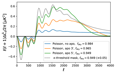
Figure 6: Correction to the lensed CMB temperature power spectrum $\tilde{C}_{l}$ for a mask consisting of an ensemble of disks of radius $3\>{\rm arcmin}$, centred on sources Poisson-sampling a underlying density field $\delta(\hat{n})$, for a total masked (unapodized) sky fraction of $1.6\%$. Shown are the cases without apodization (blue) or after apodization as indicated in the legend (orange and green). Apodization increases the masked sky fraction, and introduces a cut-off at the corresponding scale. When sampling a biased matter tracer $b\delta$, the mask traces the peaks better (for $b>1$) and all the coloured curves scale increase linearly with $b$. For this figure, $\delta$ is taken to be the lensing convergence field $\kappa$ to allow comparison with the $\kappa$-threshold mask results (black dotted, scaled by a factor 0.05; see Fig. 4). For Poisson distributed sources, even highly biased source masks give a much smaller effect than direct thresholding.

II.3 Polarization

The general result of Eq. (13) also holds for the polarization or cross-correlation, simply by using the relevant correlation functions in place of the temperature correlation function. However, for B-mode polarization, the choice of estimator is much more important. The mask-normalized pseudo-correlation functions we are analysing here correspond to deconvolved pseudo-$C_{\ell}$ estimators. It is well known that for polarization, although these estimators are unbiased, they couple cosmic variance of E-modes into B-modes due to E-to-B mixing on the cut sky. For this reason they are unlikely to be used in practice for analysing future data, where sensitivity to small B-mode signal is a major goal. It is also clear that there are likely to be many fewer polarized sources compared to temperature sources, so a much small masked sky fraction is likely Lagache et al. (2020). However, as a baseline for reference and comparison, we do briefly present a few basic results for the pseudo-correlation function estimators. These are likely to remain relevant for many E-mode power spectrum analyses, and we comment in later sections about the impact of using different estimators where the effects on the B-modes may be much smaller.

The form of the correlation function results is basically the same, but the polarization pseudopower spectra are formed from combinations of the two $\xi_{\pm}$ correlation functions. In harmonic space this still give a convolution-like effect on the power spectra: if we take the unlensed $C_{l}^{B}=0$, on large scales compared to the foreground correlation length and hole size, the result corresponding to Eq. (17) for the temperature is

$$\Delta\tilde{C}^{E}_{l}\sim-2\frac{\bar{f}}{\sigma_{f}^{2}}\int\frac{{\rm d}^{2}\bm{l}^{\prime}}{(2\pi)^{2}}\tilde{C}^{E}_{l^{\prime}}C^{\phi f}_{|\bm{l}-\bm{l}^{\prime}|}\bm{l}^{\prime}\cdot(\bm{l}-\bm{l}^{\prime})\cos^{2}(\phi_{\bm{l}^{\prime}}-\phi_{\bm{l}}),$$ (32)

$$\Delta\tilde{C}^{B}_{l}\sim-2\frac{\bar{f}}{\sigma_{f}^{2}}\int\frac{{\rm d}^{2}\bm{l}^{\prime}}{(2\pi)^{2}}\tilde{C}^{E}_{l^{\prime}}C^{\phi f}_{|\bm{l}-\bm{l}^{\prime}|}\bm{l}^{\prime}\cdot(\bm{l}-\bm{l}^{\prime})\sin^{2}(\phi_{\bm{l}^{\prime}}-\phi_{\bm{l}}).$$ (33)

For low $l$, we have the leading order result

$$\Delta\tilde{C}^{B}_{l}\sim 2\frac{\bar{f}}{\sigma_{f}^{2}}\int\frac{{\rm d}l^{\prime}}{l^{\prime}}\frac{{l^{\prime}}^{2}\tilde{C}^{E}_{l^{\prime}}}{2\pi}C^{f\kappa}_{l^{\prime}},$$ (34)

which is white and negative, compared to the standard lensing result

$$\tilde{C}^{B}_{l}\sim 2\int\frac{{\rm d}l^{\prime}}{l^{\prime}}\frac{{l^{\prime}}^{2}\tilde{C}^{E}_{l^{\prime}}}{2\pi}C^{\kappa\kappa}_{l^{\prime}}.$$ (35)

The correction can easily make the total negative on large scales if $f$ is well correlated to $\kappa$ and relatively smooth. Figure 15 in Appendix B shows numerical results for a simple test case. On the E-modes and temperature cross spectrum the effect is qualitatively similar to on the temperature spectrum, but the B-mode spectrum picks up a large bias. This large bias is a result of the way that the estimators are combining cut-sky modes, and is entirely driven by the masking effect on E-modes. Using a pure-B estimate of the power spectrum would give a much smaller result.

III Numerical results

III.1 Simulations and comparison method

We tested the accuracy of our analytic estimates against numerical simulations that model the relevant effects, in particular the extragalactic foreground emission and their correlation with CMB lensing. For this purpose we used the publicly available Websky simulation suite Stein et al. (2020) which includes maps of CMB lensing convergence $\kappa$, radio point sources, CIB, and tSZ produced from the same underlying mass distribution at $z\leq 4.5$. The mass distribution was constructed with the accelerated N-body mass-Peak Patch approach Stein et al. (2019); Bond and Myers (1996) from a 15.4 Gpc³, 12,2883 particle lightcone in a Planck 2018 cosmology. CIB and tSZ emission maps were constructed starting from the same matter distribution and using halo models matched to the latest CMB data from Planck, SPT and ACT as well as Herschel data at frequencies relevant for CMB experiments. We refer the reader to Ref. Stein et al. (2020) for more details of the semianalytic models adopted for these maps.

Since the mask-induced biases are small, and depend on the properties of the underlying matter field which is non-Gaussian, we created two sets Monte Carlo simulations of 100 lensed CMB realizations each. To build the first set, the unlensed CMB realizations were lensed using the same deflection field constructed from the Websky $\kappa$ simulation (NG set). To build the second set, the same unlensed CMB simulations were lensed with different Gaussian random realizations of the deflection field having the same angular power spectrum as the Websky $\kappa$ map (G set). We used the NG set to isolate the bias as it would appear on real data while the G set was used to compute the error bars of our measurements. Hence, the error bars displayed in the figures do not include any non-Gaussian contribution to the covariance. In the following, unless stated otherwise, error bars displayed in figures represent the error on the average measured on the G simulations.

III.2 Limiting case: 100% correlated foreground mask

As a first test we considered the extreme case of a mask constructed from a foreground that is 100% correlated with CMB lensing, creating a foreground mask $W_{\kappa}$ by simply thresholding the CMB lensing $\kappa$ field. Since the total bias is sensitive to the overall sky fraction removed by the mask, as well to the specific correlation between the mask and the convergence, we tested different configurations. To test the dependency on the sky fraction we thresholded the field masking all the pixels above a specific $\kappa$ value so that a sky fraction $f_{\rm sky}^{\rm mask}$ is removed. This generates masks with large numbers of small holes. To test the effect of the correlation scale of the deflection field and the shape of the mask, we also created masks by smoothing the $\kappa$ field with Gaussian beams of different full width at half maximum (FWHM, $\theta_{1/2}$) prior to the thresholding step. This results in more regular and connected holes due to the longer correlation length, and also effectively reduces the shot noise of the foreground map (i.e. $\kappa$) due to the finite number of particles in the Websky N-body simulation.

The bias induced by $W_{\kappa}$ is estimated as the difference between the power spectra obtained using the original (unrotated) mask, and a randomly rotated mask, both using the same NG lensed CMB realizations. The rotated mask $W_{\kappa}^{\rm rot}$ is derived from a random rotation of the original $W_{\kappa}$ so that it is uncorrelated with $\kappa$, but retains all the other nontrivial mode-coupling effects due to cut sky and hole shapes. The correlated mask bias evaluated in this way is therefore insensitive to numerical effects only due to an incomplete sky coverage. We computed the power spectrum of the masked CMB skies using a pseudo-$C_{\ell}$ method as implemented in the NaMaster package Alonso et al. (2019) and used a $C^{2}$ function (effectively a cosine) to apodize the mask to control ringing effects in harmonic space. This approach follows common practice in CMB analyses including small angular scales and is described by the analytic modelling presented in the previous sections. As we discuss in Sec. IV, alternative estimators capable of effectively recovering the information inside the holes of the mask would give different results and potentially have a reduced effect.

Figure 7 shows the measured bias from mask correlations measured in the simulations (shown as data points), compared to the semianalytic perturbative prediction described in Sec. II.1.

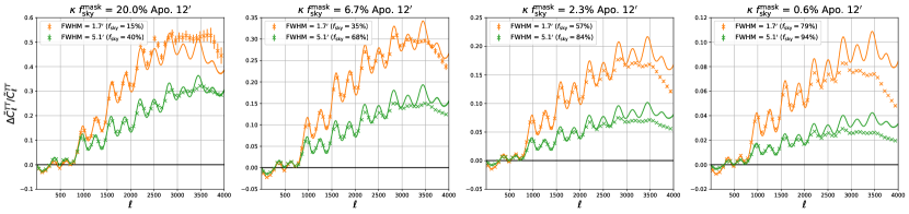
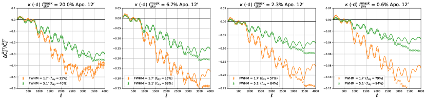
Figure 7: Bias induced by masking the lensed CMB temperature with a foreground mask generated by thresholding the Websky CMB lensing $\kappa$ field after smoothing to a scale of $1.7^{\prime}$ (orange) or $5.1^{\prime}$ (green). In the top panel data points measured from simulations are compared to perturbative semianalytic predictions in solid. Results obtained by masking different sky areas are shown in different columns. We apodized each mask with a 0.2 deg. apodization length to control ringing effects in the power spectrum estimation step. The masked area prior to apodization is reported in the title and the effective sky area after apodization used to compute $C_{\ell}^{TT}$ is shown in the legend. The bottom panel shows the bias measured on CMB simulations lensed with a deflection field with an inverted sign (NG^- set). Since the leading-order effect of the mask correlation is linear in the lensing, the bias has the opposite sign compared to the case of the top panel on scales where the leading order predictions are accurate. See Sec. III.4 for more details.

To compute the theoretical predictions we measured the required cross-spectra between the mask and the deflection field from simulations, as well as the mask auto spectrum. The semianalytic model describes the effect on large scales up to $\ell\approx 3000$ remarkably well for all the configurations considered here. This holds also for extreme cases where the relatively blue shape of the Websky $\kappa$ angular power spectrum, the presence of N-body shot-noise and the relatively large apodization length adopted, leads to the mask containing numerous tiny disconnected regions with greatly reduced effective sky area (as low as 15%, even with no Galactic plane mask). On smaller scales, the agreement between simulations and predictions gets worse, but a better fit can be achieved using the nonperturbative calculations discussed in Appendix B.

III.3 Cosmic infrared background

The CIB is produced by star-forming galaxies through the absorption of stellar radiation by dust grains which is later reemitted in the infrared. The clustering of halos, and consequently of the galaxies within, then generates the observed CIB intensity fluctuations Viero et al. (2013). In addition to providing important constraints on the physics of star formation over a wide range of redshifts and halo and galaxy masses, especially for the objects with low luminosity that cannot be studied individually, the CIB acts as an important contaminating emission at microwave frequencies. Due to its spectral energy distribution (SED) similar to thermal dust emission it is difficult to disentangle CIB and galactic dust through component separation and perfectly remove both components, in particular at small angular scales and high observing frequencies. CIB residuals then propagate to data products derived from CMB maps.

For CMB lensing and Compton $y$ maps, CIB residuals are potentially particularly harmful as they are highly correlated with the underlying cosmological signals Ade et al. (2014a, 2016a); Aghanim et al. (2016a); Song et al. (2003), and hence can bias cosmological analyses. The CIB is therefore an example of a foreground highly correlated with CMB lensing ($\gtrsim 70\%$ for $\ell\lesssim 1000$ where clustering of the emission is important). We constructed a threshold mask $W_{\rm CIB}$ following the procedure outlined in the previous section starting from the Websky CIB map at 217GHz. This frequency was chosen as it is the highest relevant frequency typically used for CMB power spectrum analysis based on multi-frequency cross-correlation as done for e.g. Planck. The Websky maps are based on a halo model of CIB previously used to fit Herschel and Planck data Shang et al. (2012); Viero et al. (2013); Ade et al. (2014b). The rest-frame SED of CIB in these halos accounts for mass, frequency and redshift evolution as well as frequency decorrelation, and was normalized to reproduce the Planck CIB at 545 GHz Ade et al. (2014b); Aghanim et al. (2016b). While improvements to this model have been recently presented in the literature Maniyar et al. (2021), it is sufficient to reproduce with good accuracy all the measurements available in the literature from Planck and Herschel data between 143 GHz and 857 GHz (see Stein et al. (2020) and references therein for more details). Figure 8 shows the correlated mask bias measured from simulations adopting the same $C^{2}$ function of the previous section and using two different apodization lengths ($3^{\prime}$ and $12^{\prime}$), compared to our semianalytic perturbative predictions.

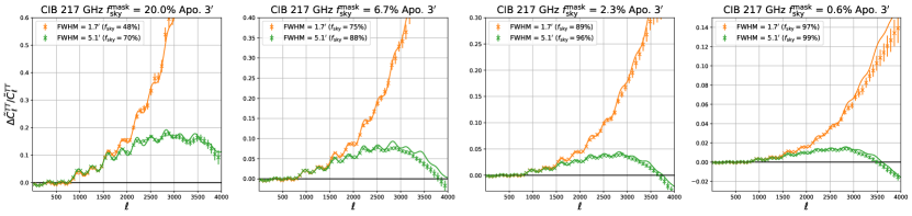
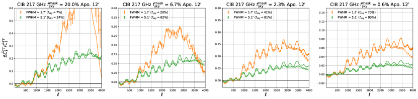
Figure 8: Bias induced by masking the lensed CMB temperature with a foreground mask generated by thresholding the CIB map at 217 GHz of the Websky suite after smoothing to a scale of $1.7^{\prime}$ (orange) or $5.1^{\prime}$ (green). Data points show the measurements of the bias on simulations while perturbative semianalytic predictions are shown in solid lines. Masks with different sky fractions are shown in different columns. The top row shows results with $3^{\prime}$ mask apodization tapering function, the bottom row using a larger $12^{\prime}$ apodization (giving substantially larger masked areas as shown in the legend).

As for the case of the $W_{\kappa}$ mask, the theoretical predictions match the simulation measurements very well up to scales $\ell\lesssim 2500$. The amplitude of the mask bias at small scales has a peak and then decreases on scales smaller than the characteristic scale imposed by the mask hole size. Qualitatively this turnover is similar whether the larger hole size is caused by apodization, or by thresholding a smoothed CIB map. When masking the CIB peaks without applying any smoothing of the CIB maps prior to thresholding (orange lines and points in Fig. 8), there are many very small holes due to the relatively blue shape of the CIB angular power spectrum. A larger apodization scale increases the fraction of sky that is masked for fixed underlying hole distribution, increasing the bias on larger scales (where noise and foreground power is lower, and therefore potentially more important in the analysis of real data).

Although masks on real data are usually not designed to remove peaks of CIB emission per se, the case where we masked the highest peaks so that only the 0.6% of the sky is removed is of particular interest. Infrared sources that are local dusty galaxies are expected to have a low correlation to CMB lensing due to the short path length. However, chance radial alignments of sources for the CIB, high-redshift protoclusters, and lensed high-redshift galaxies, may make up an important fraction of the point sources detected in CMB maps Vieira et al. (2010, 2013), all of which may have a significant correlation to the line of sight CMB lensing Bianchini et al. (2015, 2016); Aguilar Faúndez et al. (2019). The brightest of these objects are usually removed by point sources masks (see later Sec. III.5). Despite the reduced masked sky area, the bias in this case is potentially significant and could lead to important detectable effects as we will see in the following sections.

There are however several caveats to our analysis. The Websky CIB simulations do not model specifically the effect of Poisson shot noise for the brightest sources nor include lensing of the infrared galaxies, which potentially make up a significant fraction of the detected objects Negrello et al. (2010); Gonzalez-Nuevo et al. (2012), especially the brightest one. Moreover, objects located at very high redshift above the maximum redshift probed by the LSS included in Websky ($z_{\rm max}=4.5$), despite being very rare, can still retain a nonzero correlation with CMB lensing as CMB lensing kernel has a non-negligible amplitude in that regime (see e.g. Wilson and White (2019) for a discussion on high-redshift object cross-correlation in the optical band).

III.4 Thermal SZ

Observation of the tSZ effect, the inverse Compton scattering of CMB photons by free electrons, is a well established way to construct roughly mass-limited samples of galaxy clusters that are independent of redshift and thus very powerful cosmological probes Birkinshaw (1999); Carlstrom et al. (2002); Mroczkowski et al. (2019). tSZ clusters mark out large-scale density peaks, and as such have substantial correlation to CMB lensing, at the $30-50\%$ level Hill and Spergel (2014), and the emission also follows highly non-Gaussian statistics Thiele et al. (2019); Coulton et al. (2018). If tSZ clusters are masked out, the CMB lensing-mask correlation can be substantial.

Current CMB surveys from the ground and from space have blindly detected approximately 3200 tSZ clusters with redshift measurements to date Ade et al. (2016b); Bleem et al. (2020); Hilton et al. (2020). Due to its characteristic spectral signature, tSZ emission can be subtracted from CMB maps using component separation. However, this becomes difficult on small scales where noise becomes important, and foreground-cleaning residuals are less simple to model. The tSZ signal is therefore usually not cleaned for CMB power spectrum analysis, instead its contribution to the observed power spectra is accounted for in the model. Nevertheless, to minimize complex foreground residuals, for various higher-point statistics (including CMB lensing reconstruction) it is often useful and common practice to remove some of this source of highly non-Gaussian signal by masking the SZ clusters (see e.g. Osborne et al. (2014)). In this case it may also be important to understand what happens to the two-point statistics over the remaining unmasked area. Planck data were shown to be robust to these effects Aghanim et al. (2020), however future ground-based surveys such as Simons Observatory Aguirre et al. (2019) (SO) and CMB-S4 Abazajian et al. (2019a) (S4 hereafter) will detect one order of magnitude more clusters and thus cluster masking might potentially soon become a more significant issue.

We followed the same procedure outlined in previous sections and constructed a mask based on the thresholding of the Websky tSZ Compton $y$ parameter map $W_{y}$. The Websky simulation models the tSZ emission starting from the dark matter halos identified in the simulation, and applies a halo model construction including the effects of non-thermal processes such as radiative cooling, star formation, supernova and AGN feedback in the pressure profile Battaglia et al. (2012). As a result, the $y$ map is highly non-Gaussian with the skewness and kurtosis of its 1-point PDF having values significantly above 1.

In Fig. 9 we show the comparison of our theoretical predictions with the simulation measurements.

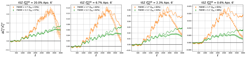
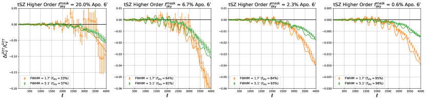
Figure 9: Top: bias induced by masking the peaks of the tSZ emission (after smoothing to a scale of $1.7^{\prime}$, orange, or $5.1^{\prime}$, green) on the lensed CMB temperature as measured on simulations compared to perturbative leading order analytic predictions (solid line). Masks with different sky fractions are shown in different columns. We adopted a $6^{\prime}$ apodization length for the mask tapering function. Bottom: measurement on simulations of the even higher-order biases responsible for the discrepancies between the leading order predictions and the simulation results shown in the upper panel. Approximate analytic predictions of the second-order terms are shown as solid lines and described in Sec. III.4.

Compared to the case of $\kappa$ and CIB thresholding, the agreement between the perturbative model and simulation results is worse, with significant discrepancies observed already at multipoles $\ell\approx 2500$ and reaching a factor between 2 to 4 at $\ell\approx 4000$ in particular when only the highest peaks are masked (right panel). For more aggressive masks where a significant fraction of the peak is masked however the agreement (left panel) between simulations and analytic predictions improve substantially. Since the bulk of the tSZ emission is localized in highly clustered and dense regions at relatively low redshift for a threshold that is sufficiently small, $W_{y}$ contains holes with a larger angular size around the overdensity corresponding to the galaxy cluster. The masked region at each cluster may therefore remove a significant area of high lensing signal associated with the cluster (rather than just a small area at the very peak of the overdensity). We therefore checked whether higher-order effects beyond the linear term modelled in the previous section could be responsible for the observed discrepancy, for example from the reduction in lensed CMB signal over the cluster mask.

To test higher-order effects we constructed another set of lensed CMB simulations with the same masks as the NG set, but lensed with a deflection field with an inverted sign. We refer to this set of simulations as NG^- in the following. Since the leading-order effect of the mask correlation is linear in the lensing, in these maps it should have opposite sign (see Fig. 7). Higher-order effects that are quadratic or involve a higher even power of the lensing can be isolated on simulations using the half sum of the mask biases measured on the NG and NG^- sets using the same threshold mask for both NG and NG^-. In the bottom panel of Fig. 9 we show that higher-order effects induce a negative correction to the leading order predictions that explains the discrepancy. When only a reduced fraction of the sky is masked, the higher-order effects become important at $\ell\approx 2000$ and suppress the bias by a factor of 4 compared to the leading order predictions at $\ell\approx 4000$. In the limiting case where we mask a large fraction of the sky, the corrections become relevant at progressively smaller angular scales and their relative importance is reduced.

Corrections that are quadratic in the lensing largely account for a change in the underlying lensed CMB power spectrum due to the masking of areas where the lensing is larger. An approximate analytic estimate of this higher-order bias can be obtained by computing the lensed CMB power spectrum (approximately a convolution of the CMB lensing and the unlensed CMB power spectra) where the CMB lensing power spectrum is derived from the lensing convergence power spectrum computed over the masked sky using the $W_{y}$ mask. Figure 9 shows that this simple model describes the effect seen in the simulations quite accurately (a more accurate analytic calculation, including all orders for a Gaussian foreground, is described in Appendix B).

III.5 Radio point sources

The dominant population of bright point sources detected at CMB frequencies are AGN-powered radio sources emitting synchrotron radiation through acceleration of relativistic charged particles de Zotti et al. (2010). The details of the observed emission law of such sources (whose intensity typically decreases as frequency grows) depends on the orientation of the observer relative to the axis of the characteristic jets emerging from the central black hole Padovani et al. (2017). Because the synchrotron emission is polarized, some of the sources detected in temperature also have a counterpart in CMB polarization maps. So far only a minor fraction of the detected sources in temperature are polarized, but the situation is expected to change in the coming years where hundreds of object will be identified in deep polarization maps Puglisi et al. (2018); Lagache et al. (2020). These are potentially an important obstacle to the exploitation of small scale E-mode polarization data as well as large scale B-mode polarization if the tensor-to-scalar ratio $r$ is sufficiently low. As such, all these sources are systematically masked in CMB temperature power spectra analyses. Polarization data can be masked separately (using only the detected objects in polarization) or together with temperature data using the same mask Planck Collaboration XI (2015); Choi et al. (2020); Sayre et al. (2020); Henning et al. (2018). Other analyses studying statistically anisotropic effects in CMB maps (e.g. CMB lensing or birefringence reconstructions) adopted different approaches, ranging from keeping the same mask as in power spectrum analysis or using dedicated source-subtracted or inpainted maps Aghanim et al. (2020); Bianchini et al. (2020); Wu et al. (2019); Aiola et al. (2020); Naess et al. (2020).

Halos hosting radio sources, and therefore the radio source distribution (especially the low flux component), correlate with large-scale structure and hence with the tSZ emission, CMB and galaxy lensing and CIB Holder (2002); Shirasaki (2019); Allison et al. (2015); Dwek and Barker (2002). The relatively low amplitude of the clustered component of $\sim 10{\rm s}-100{\rm s}$ mJy radio sources detected in current generation CMB maps, means that for current masked source densities the mask can be approximated as uncorrelated to the lensing to good accuracy. We used Websky radio sources mock catalogues to test that this is indeed the case, and whether this assumption breaks down for future experiments.

The radio-source mocks use the halos identified in the simulation box of Websky to implement a halo occupation distribution (HOD) for the Fanaroff-Riley Class I (FR- I) and Class II (FR-II) galaxies described in Wilman et al. (2008); Sehgal et al. (2010). The HOD models the occupation numbers of FR-I and FR-II populations as broken power laws and asymmetric Gaussians and a luminosity function given by a broken power law with a luminosity cut-off set to reproduce the luminosity function at 151MHz. The constructed HOD is then resampled to match the observed flux counts $n(S)={\rm d}N/{\rm d}S$ while keeping the same rank ordering of the original catalogue, mixing in practice HOD and abundance matching techniques (see Li et al. (2020) for more details). The constructed catalogues reproduce with good precision the Planck number counts at frequencies $\nu\leq 143$GHz where the radio galaxies dominate the DSFGs population.

To build the RS mask for a given experiment we started from the simulated radio catalogues and selected the sources that have a measured flux above the detection limit of a particular experiment. We focused on Planck , SO and S4, and for each of these we selected the sources in the three frequency bands most relevant for small-scale power spectra measurements. We label these LOW, MID, HIGH, with each having a different flux limit and resolution as shown in Table 1. The properties of the selected galaxy samples for each experiment are summarized in Fig. 10.

Channel	$\nu$ (GHz)	Intensity flux cut (mJy)	$\theta_{1/2}$ (arcmin)
Planck LOW	100	232	9.69
Planck MID	143	147	7.30
Planck HIGH	217	127	5.02
SO LOW	93	4.37	2.2
SO MID	145	5.03	1.4
SO HIGH	225	9.88	1.0
S4 LOW	95	2.82	2.2
S4 MID	143	1.98	1.4
S4 HIGH	220	4.37	1.0

Table 1: Point source intensity flux cut values and resolution of the different frequency channels and experiments considered in this work. See Lagache et al. (2020); Planck Collaboration XI (2015); Aguirre et al. (2019) for more details.

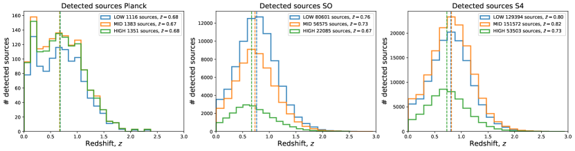
Figure 10: Distributions of the Websky simulation radio galaxy population at different frequencies that would be detected using the flux limit for different experiments. Numbers here are over the full sky and are masked in our full-sky analysis. The number of sources detected over the full sky is shown in the label while the median redshift is shown as a dashed vertical line. See Table 1 for the specification of the LOW, MID, and HIGH frequency channels.

In the literature, different experiments adopted different choices for how to mask point sources. Planck masked a circle of radius $3\sigma=3\theta_{1/2}/\sqrt{8\log 2}\approx 1.3\theta_{1/2}$, where $\theta_{1/2}$ is the FWHM of the beam of each frequency channel and a Gaussian tapering function with $30^{\prime}$ apodization length Planck Collaboration XI (2015). Ground-based experiments adopted more conservative choices. ACTpol used holes of a radius of about $\sim 3.5\theta_{1/2}$ radius hole at 98GHz and 150GHz with a sine apodization having a length ranging between $10^{\prime}$ to $15^{\prime}$ Choi et al. (2020). SPTpol typically masked the sources with a fixed $5^{\prime}$ radius circle (which is $\sim 3-5\theta_{1/2}$ at 95-220GHz) and a cosine apodization with $5^{\prime}$ apodization length Bianchini et al. (2020). For small-scale temperature analysis, they adopted a different masking procedure with larger holes for the brightest sources Reichardt et al. (2020). For wide surveys such as Planck  or ACTpol Wide, the fraction of observed sky masked by sources before apodization amounts to $\sim 0.4\%$ while deep surveys like SPTpol and ACT deep removed a few percent of the observed sky. We investigated the impact of different setups in terms of apodization and hole size, and Fig. 11 summarizes our findings.

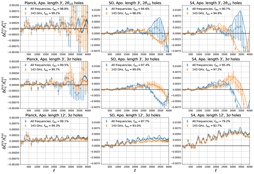
Figure 11: Effect of masking radio sources for different experiments considered in this work (left to right). The MID frequency channel is shown in orange, and the mask derived by taking the product of the masks at each considered frequency channel is shown in blue. Simulation measurements are shown as data points and the semianalytic theory prediction in solid. Different hole sizes are displayed in the top and middle panel. The point source masks were apodized with a $C^{2}$ tapering having an apodization length of $3^{\prime}$ (upper and middle panel) and $12^{\prime}$ for the bottom one.

The clustering of the selected galaxies is dominated by the shot noise for all the selected galaxy samples. The mean cross-correlation with CMB lensing is 5%, below 10% on all angular scales for the deepest sample of S4, and one order of magnitude lower for Planck. The formalism based on Poisson sampling of the density field (see Sec. II.2.2) would thus be appropriate if one had to model the effect from first principles. In Fig. 11 we use the empirical model of Sec. II.1 to compute the analytic predictions. A $C^{2}$ apodization of the mask holes is used to measure the effects on simulations for consistency with the results of the previous sections.

For the case of masks with $3\sigma$ hole radius, and the union mask that removes sources detected at all frequencies (which largely overlap between frequency channels), for Planck we find a negligible effect of the order of $\sim 0.01\%$. For SO and S4 however, the effect becomes comparable to the cosmic variance uncertainty and therefore becomes relevant. Increasing the hole radius to $2\theta_{1/2}$ makes the bias shape change significantly, especially at small angular scales where it can grow to about 1% and change sign. Increasing the apodization length potentially has a more important effect as all scales are affected by the increased masked area. An apodization such as that of adopted by Planck Planck Collaboration XI (2015) can increase biases by a factor two, however for the specific case of Planck shown here, it still keeps the bias below the detection threshold. If instead we mask only the sources detected at a given frequency, we found that the LOW and MID frequency channels are the ones most affected, as they are the ones where the effect is larger and/or have the lowest flux detection threshold.

More conservative approaches to point source masking, as typically adopted in the analysis of ground-based experiments mentioned above, where the hole radius exceeds the $2\theta_{1/2}$ value considered in this work and wider apodization lengths are employed, will lead to a significant increase of the bias and a strong detection if unmodelled. At the SO and S4 level of sensitivity such strategies will need to be reconsidered as it may become necessary to find a compromise between data loss, increase of the mask-induced bias, and foreground contamination. In all cases, however, our analytic model describes the results of simulations well and can be used to estimate or mitigate the bias when required.

As shown in Appendix B, the mask bias observed on E-modes is roughly a factor 2 lower compared to the one observed in the temperature power spectrum. If a common mask between temperature and polarization is adopted, we expect the bias to become relevant for high-sensitivity analysis of small-scale E-mode polarization and be negligible for B-modes on scales $\ell\gtrsim 200$ if a pure-pseudo power spectrum (or more optimal Tegmark and de Oliveira-Costa (2001)) method is used Smith (2006); Grain et al. (2009). In the case of a pure-B estimator the residual observed bias comes mainly from higher-order masking effects suppressing the lensed B-mode power, while the larger bias at linear order involving E-modes converting to B-modes is naturally removed. An accurate evaluation of the bias on the large angular scale B-mode power from pure pseudo-$C_{\ell}$ methods would depend on the details of the apodization length of the mask. This can be highly nontrivial in presence of masks with complex boundaries, such as those removing radio point sources, and should anyway be optimized given an experimental noise level and a choice of multipole binning to minimize the total B-mode variance Ferté et al. (2013, 2015). This is beyond the scope of this paper and we leave this exercise for future work. However, in Fig. 12 we show an example of the effect of the B-mode purification on the mask bias for the limiting case of a $W_{\kappa}$ mask. For the more realistic case of a mask that removes radio sources detected at all frequencies, the B-mode power bias for the pure estimator is $\sim 10-20\%$ at $\ell\approx 200$ for S4.

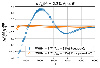
Figure 12: Lensing-induced mask bias on the B-mode angular power spectrum for a standard pseudo-$C_{\ell}$ estimator (blue) and for a pure pseudo-$C_{\ell}$ estimator (orange). Because the major source of the bias at leading order is a conversion from E to B-modes, the pure estimator removes almost entirely the bias observed with the standard estimator. The two estimators generate a very similar bias at small scales where the bias is mainly sourced by higher-order terms in the lensing (e.g. the suppression of lensing power due to peak masking).

IV Impact on current and future data sets

IV.1 Detectability, diagnostics and mitigation

Although the level of the bias can easily be calculated from simulations, in practice it is usually not straightforward to reliably simulate very precisely what is being masked, so some kind of internal measurement or diagnostic would be useful. Fortunately, because the effect is linear in the lensing, it is quite distinctive.

We can expect methods that reconstruct the CMB inside the holes, such as inpainting or CMB Wiener filtering, to be quite effective at reducing the bias (or affecting its shape) if the mask is not too large. This is because the temperature in a small hole can be predicted accurately by using the large-scale temperature modes that are well measured outside the mask. The correlation between the temperature value in the masked hole and the surrounding lensing (see Fig. 2) would then be mostly recovered, giving little net bias. The temperature reconstruction may itself bias the result, but in a very different way that allows for consistency checks. The effect can also be isolated in cross-correlation of masked and unmasked (or inpainted) maps, where the bias appears on large-scales with half the amplitude. This has the advantage of not picking up mean white foreground noise from the unmasked foreground peak or some effects of inpainting errors, allowing a direct comparison with the masked auto spectrum.

For example, simulations suggest that the Planck  point-source mask of $f_{\rm sky}\sim 2\%$ Planck Collaboration XI (2015) could bias cosmological parameters by up to about $1\sigma$ if the mask were highly correlated to the lensing, but assessing exactly the level of correlation from purely theoretical considerations or simulation is difficult. We can instead directly assess the size of the bias by looking at cross-spectra between masked and inpainted maps. Specifically, we consider the difference of power spectra $\rm{SMICA}\times\rm{SMICA}-\rm{SMICA}\times\rm{SMICA}^{\prime}$, where $\rm{SMICA}$ is the foreground-cleaned SMICA temperature map Akrami et al. (2020) masked by one of the likelihood masks including point source mask, and $\rm{SMICA}^{\prime}$ is the SMICA map only masked by the galactic mask and inpainted elsewhere. To avoid noise bias in the power spectrum, the first and second map can be taken from different half-mission splits. For the various frequency masks the smoothed difference is always $\Delta D_{\ell}<1\mu{\rm K}^{2}$ at $1000<\ell<2000$ and $<4\mu{\rm K}^{2}$ on larger scales (with much of the variation expected from cosmic variance over the differing areas), suggesting the level of bias is safely negligible for the default Planck  masks.

The effect can also be tested using an estimate of the deflection field over the unmasked area to empirically estimate $\bar{\Delta}(r)$ (Eqs. (9), (11)). For Planck two good tracers of the lensing field are available: the lensing reconstruction Aghanim et al. (2020) (on large scales) and the cosmic infrared background (which is highly correlated to lensing and well-measured by Planck on smaller scales), which can be used to estimate $\bar{\Delta}(r)$ and hence the expected impact on the power spectrum. In either case we find these semianalytic predictions consistent with zero. Each method of assessing the bias has some caveats, but taken together there seems to be good consistency with negligible bias for Planck parameters due to mask-lensing correlations. This is consistent with the expectation that the mask is dominated by Poisson radio sources, which have negligible impact given the number densities of sources masked by Planck, and nearby galaxies that are only weakly correlated to the CMB lensing. We reach the same conclusion trying to estimate the $\bar{\Delta}(r)$ on ACT DR4 Aiola et al. (2020) D56 and D8 deep regions. For higher-resolution and forthcoming data, where substantially more sources may be resolved, mask bias consistency checks may be much more important.

On the other hand, we can easily detect biases in Planck’s SMICA maps when using a modified mask designed for the purpose. Fig. 13 shows results when masking additional $5\%$ of the sky with a foreground threshold mask. The points show the difference in the $\rm{SMICA}$ map power spectrum, as calculated on the union of the Planck likelihood masks at 143 and 217GHz ($f_{\rm sky}=43\%$), after masking this additional $5\%$ of the sky by directly thresholding on a foreground map taken here to be the (noisy, and beam-convolved) Planck CIB observations as captured by the GNILC Aghanim et al. (2016c) map at 545GHz. The error bars are estimated for each multipole bin from the empirical standard deviation of the spectrum. The blue curve shows the analytic prediction for the bias as obtained with the threshold model of Sec. II.2.1. Along with the foreground autospectrum, the prediction requires its cross-spectrum to the lensing potential. We have used the empirical cross-correlation of the GNILC map to Planck 2018 publicly available lensing map (Aghanim et al., 2020, MV estimate) for this purpose. This could be viewed as a rather nontrivial consistency check of our analysis and several Planck products.

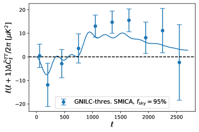
Figure 13: Difference between Planck $\rm{SMICA}$ data power spectra estimated on the Planck likelihood mask and after removing an additional $5\%$ of the sky, directly thresholding on the GNILC CIB map at $545$GHz. The solid line is the analytic prediction using the Gaussian foreground thresholding model in this paper, where the cross-spectrum of the foreground to the lensing potential is obtained from the cross-spectrum of GNILC map to the Planck 2018 lensing MV lensing potential quadratic estimate.

IV.2 Forecasts for future experiments

Despite not being detectable on current data sets, in the previous sections we have shown that correlated masks can introduce substantial biases on the power spectrum if not accounted for, and they may be import for forthcoming more sensitive experiments that measure small angular scales. We therefore calculated the detectability of the biases induced by masking of tSZ, CIB and radio sources for SO and S4 assuming a sky coverage of $f_{\rm sky}=40\%$ and the realistic publicly available noise power spectra in temperature and polarization after a component separation procedure based on a standard internal linear combination algorithm. In Fig. 14 we show the detectability of the bias in terms of achievable detection significance as a function of the highest multipole included in the analysis. This approach is simplified and assumes the perfect knowledge of the CMB power spectrum and, if employed, of the nuisance parameters used to describe the foreground residuals. As such, a detectable bias should be interpreted as showing that it is necessary to model the effect to be sure the inference of remaining cosmological (or nuisance) parameters is not biased. We note here that the masks are unapodized.

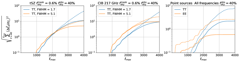
Figure 14: Detection significance of the mask bias as a function of maximum multipole $\ell_{\rm max}$ included in the analysis for different sources for future high-resolution ground-based experiments. SO is shown in solid line while S4 is shown in dashed line. For both surveys we assumed a sky coverage of $f_{\rm obs}=40\%$. Unlike Figs. 8, 9, 11, no apodization was applied to the mask prior to the computation of the power spectrum bias. This choice is conservative as it allows us to retain the largest observed sky area for a given mask and thus a smaller bias on the majority of angular scales. The fraction of the sky area removed by masks based on foreground thresholding is shown in the title as $f_{\rm sky}^{\rm mask}$. The significance reported is assuming the full sky CMB spectra are known perfectly (and an error model only accounting for foreground-cleaned noise).

If tSZ and the brightest regions of CIB emission (which are considered here as proxy of DSFGs and covering only $0.6\%$ of the sky) are masked, biases on $\tilde{C}_{\ell}^{TT}$ will be detected with a statistical significance well above $5\sigma$ for both SO and S4. For RS masking we assumed that a joint mask removing all sources detected at any frequencies with a hole radius of $\sim 1\theta_{1/2}$ is applied to both temperature and polarization. Considering only multipoles $\ell\lesssim 3000$ where extragalactic foreground residuals become important, only S4 would detect the effect above $5\sigma$ in $\tilde{C}_{\ell}^{TT}$ while for SO the detection significance is reduced to $\sim 2\sigma$. Measurements of $\tilde{C}_{\ell}^{EE}$ are less affected by the bias and should remain insensitive to it at SO sensitivity, while S4 will need to account for the effect as it should be able to measure it at $\sim 3\sigma$. The size of the bias for $\tilde{C}_{\ell}^{BB}$ is highly dependent on the choice of the estimator. Standard pseudo-$C_{\ell}$ estimators not accounting for E-to-B leakage due to partial sky coverage in the E-B separation will lead to a very significant detection of the bias also on subdegree scales. However, estimators that remove the E-to-B leakage, such as the pure-pseudo-$C_{\ell}$, can remove the majority of the bias and leave the residual effect below the detection threshold. Except on scales smaller than the smoothing scale for the mask, the effect on the temperature and E-mode power spectra is mainly an increase in power at small angular scales. This is likely to partly degenerate with the spectral index $n_{\rm s}$ and other parameters affecting the damping tail, so any analysis neglecting the effect may misestimate these parameters. We stress however that for a given noise level, the quantitative impact of the mask bias in the analysis of real data is ultimately dependent on the details of the final analysis mask and thus on the interplay between the shape of the bias and cosmological, foreground and other nuisance parameters.

V Conclusions

We have shown that masks that are correlated to lensing can potentially give large biases in pseudo-$C_{\ell}$ power spectrum estimators, even if the masked sky area is small. To a good approximation, this results from a scale-dependent demagnification causing an efficient transfer of power from large to small scales. We discussed analytic models which accurately describe the effect of simple masks, and provided a recipe to estimate the bias empirically on simulations or data. We verified on simulations that the predicted change in the CMB power spectra is accurately capturing the main effect of the mask bias, with no significant change to the power spectrum covariances identifiable above the Monte Carlo noise. For current data, where masked source densities are relatively low and CIB and tSZ are usually not masked, the bias appears to be safely negligible. For future data, with much larger populations of resolved sources, care will be required to either include the correlated mask bias in the model, or ensure that mask hole sizes and number densities are sufficiently low that the bias remains negligible.

The bias from masking radio sources is relatively low because the Poisson sampling ensures a mask hole population tracing the background galaxy density, rather than correlating strongly with the density perturbations. However, for the high radio source densities expected in fourth-generation CMB observations, this may also start to become marginally important. If tSZ clusters (or CIB peaks) are included in the mask, the effect could be much larger, producing highly significant biases in the power spectra if left unmodelled. For these contaminants foreground modelling and cleaning is likely to remain the best approach, rather than masking. However, non-Gaussianity and lensing studies that choose to mask these sources may have to also carefully account for the induced change in the power spectrum over the remaining area. We discuss in detail the effect on lensing estimation in our companion paper Lembo et al. . A detailed study of the impact on large-scale CMB polarization and delensing is left for future work.

Appendix A Correlation function estimators and averages with binary masks

If we define the correlation function on a masked sky by the expectation between unmasked points (assuming a binary mask) we have

$$\tilde{\xi}(\bm{x},\bm{x}^{\prime}) \equiv \int{\rm d}\tilde{T}(\bm{x}){\rm d}\tilde{T}(\bm{x}^{\prime})\,\tilde{T}(\bm{x})\tilde{T}(\bm{x}^{\prime})$$ (36)

$$\quad\times P(\tilde{T}(\bm{x}),\tilde{T}(\bm{x}^{\prime})|{W}(\bm{x})=1,{W}(\bm{x}^{\prime})=1)$$

$$= \int{\rm d}\tilde{T}(\bm{x}){\rm d}\tilde{T}(\bm{x}^{\prime})\left[\tilde{T}(\bm{x}){W}(\bm{x})\tilde{T}(\bm{x}^{\prime}){W}(\bm{x}^{\prime})\right]$$

$$\times P(\tilde{T}(\bm{x}),\tilde{T}(\bm{x}^{\prime})|{W}(\bm{x})=1,{W}(\bm{x}^{\prime})=1).\qquad$$

For a mask defined on statistically isotropic fields, for $\bm{x}$ and $\bm{x}^{\prime}$ separated by $r$ we have

$${\xi_{\rm mask}}(r) \equiv\langle{W}(\bm{x}){W}(\bm{x}^{\prime})\rangle$$

$$=\int{\rm d}W(\bm{x}){\rm d}W(\bm{x}^{\prime})W(\bm{x})W(\bm{x}^{\prime})P({W}(\bm{x}),{W}(\bm{x}))$$

$$=P({W}(\bm{x})=1,{W}(\bm{x}^{\prime})=1).$$ (37)

The correlation function for unmasked points then becomes

$$\tilde{\xi}(r) =\int{\rm d}\tilde{T}(\bm{x}){\rm d}\tilde{T}(\bm{x}^{\prime})\left[\tilde{T}(\bm{x}){W}(\bm{x})\tilde{T}(\bm{x}^{\prime}){W}(\bm{x}^{\prime})\right]$$

$$\qquad\times\frac{P(\tilde{T}(\bm{x}),\tilde{T}(\bm{x}^{\prime}),{W}(\bm{x})=1,{W}(\bm{x}^{\prime})=1)}{P({W}(\bm{x})=1,{W}(\bm{x}^{\prime})=1)}$$

$$=\frac{1}{{\xi_{\rm mask}}(r)}\left\langle\tilde{T}(\bm{x}){W}(\bm{x})\tilde{T}(\bm{x}^{\prime}){W}(\bm{x}^{\prime})\right\rangle,$$ (38)

This is the same as the pseudocorrelation function for the full masked sky normalized by the mask correlation function.

From a single masked sky of data we can estimate the correlation function by an average over the unmasked sky

$$\hat{\tilde{\xi}}(r) \equiv\left\langle\tilde{T}(\bm{x})\tilde{T}(\bm{x}+\bm{r})\right\rangle_{\bm{x},\phi_{r},\rm{unmasked}}$$

$$=\frac{\left\langle({W}\tilde{T})(\bm{x})({W}\tilde{T})(\bm{x}+\bm{r})\right\rangle_{\bm{x},\phi_{r},{\rm all}}}{{\left\langle{W}(\bm{x}){W}(\bm{x}+\bm{r})\right\rangle}_{\bm{x},\phi_{r},{\rm all}}},$$ (39)

where angle brackets here denote sums over pairs of points on a fixed sky, mask and area divided by the number of pairs of points in that area. Since $\langle\hat{\tilde{\xi}}(r)\rangle=\tilde{\xi}(r)$, the expectation of this estimator is also given by Eq. (38). So for a binary mask, the expectation of the ratio in Eq. (39) is the same as the ratio of the expectations in Eq. (38).

Appendix B Nonperturbative and exact results

We can decompose the difference in the deflection angles $\bm{\Delta}\equiv{\bm{\alpha}}-{\bm{\alpha}}^{\prime}$ at two points $\bm{x}$ and $\bm{x}^{\prime}$, into a part correlated with $f(\bm{x})$, $f(\bm{x}^{\prime})$ and a part that is not, $\bm{n}$,

$$\alpha_{i}-\alpha_{i}^{\prime}=n_{i}-\xi^{f\alpha_{i}}(r)\frac{(f(\bm{x})+f(\bm{x}^{\prime}))}{\sigma_{f}^{2}+\xi_{f}(r)}.$$ (40)

From Eq. (4) this gives

$$\tilde{\xi}_{\rm masked}(r)=\int\frac{{\rm d}^{2}\bm{l}}{(2\pi)^{2}}C_{l}e^{i\bm{l}\cdot\bm{r}}\left\langle e^{i\bm{l}\cdot\bm{n}}\right\rangle\\ \left\langle\exp\left(-i\bm{l}\cdot\hat{\bm{r}}\frac{\xi^{f\alpha_{r}}(f(\bm{x})+f(\bm{x}^{\prime}))}{\sigma_{f}^{2}+\xi_{f}(r)}\right){W}(\bm{x}){W}(\bm{x}^{\prime})\right\rangle,$$ (41)

where the second average is now only a 2D integral over the foreground field values. Note that

$$\langle n_{i}n_{j}\rangle=\langle\Delta_{i}\Delta_{j}\rangle-2\frac{\xi^{f\alpha_{i}}(r)\xi^{f\alpha_{j}}(r)}{\sigma_{f}^{2}+\xi_{f}(r)},$$ (42)

so that

$$\left\langle e^{i\bm{l}\cdot\bm{n}}\right\rangle=e^{-{\textstyle\frac{1}{2}}\left\langle(\bm{l}\cdot\bm{n})^{2}\right\rangle}=e^{-{\textstyle\frac{1}{2}}\langle(\bm{l}\cdot\bm{\Delta})^{2}\rangle}\exp\left(\frac{\left(\bm{l}\cdot\hat{\bm{r}}\xi^{f\alpha_{r}}(r)\right)^{2}}{\sigma_{f}^{2}+\xi_{f}(r)}\right).$$ (43)

The remaining complex exponent on the second line of Eq. (41) is small, since $l\xi^{f\alpha_{r}}/\sqrt{\sigma_{f}^{2}+\xi_{f}(r)}\ll 1$ for cases of interest at $l\ll 10^{4}$, suggesting a leading-order expansion should be accurate.

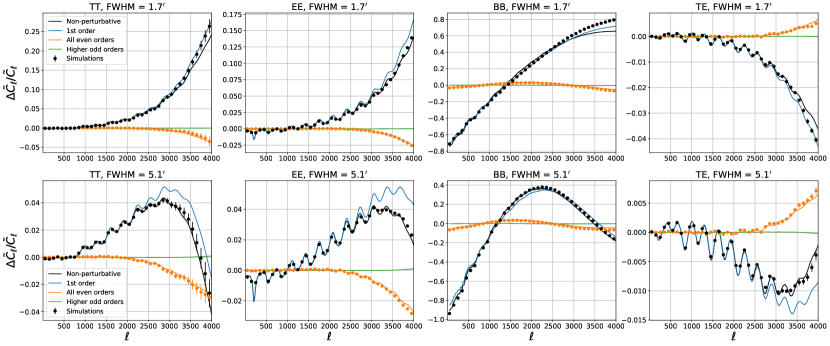
Figure 15: Total prediction for the fractional bias on the CMB power spectra (black) together with perturbative contributions of order 1 to 3 in $C_{\ell}^{f\alpha}$ (blue, orange and green), for an $f_{\rm sky}=97.7\%$ mask built thresholding $f$, the convergence map smoothed with a beam of $1.7\,{\rm arcmin}$ (top, SO-like) or $5.0\,{\rm arcmin}$ (bottom, Planck-like). The predictions are for deconvolved pseudo power spectra, where the E-modes dominates both polarization spectra biases. E/B-separated or more optimal polarization estimators would produce a much reduced BB bias. In the case of TE, instead of showing the fractional deviation we plot $\Delta\tilde{C}_{\ell}^{TE}/\sqrt{\tilde{C}_{\ell}^{TT}\tilde{C}_{\ell}^{EE}}$, which is the relevant ratio for CMB likelihoods. Note that on small scales $\tilde{C}_{\ell}^{TE}$ is mainly negative, so the oppositely signed bias term has qualitatively the same effect on the relative size of the signal as for the autospectra. In all curves the Gaussian lensing effects are exactly accounted for. The biases measured in simulations are shown with a dot marker. The orange points that isolate even higher-order effects have been computed using the method outlined in Sec. III.4.

Expanding perturbatively to lowest order in $\xi^{f\alpha_{r}}$ and using

$$\left\langle(f(\bm{x})+f(\bm{x}^{\prime})){W}(\bm{x}){W}(\bm{x}^{\prime})\right\rangle=\\ \left(\sigma_{f}^{2}+\xi_{f}(r)\right)\left\langle\frac{\partial{W}(\bm{x})}{\partial f(\bm{x})}{W}(\bm{x}^{\prime})+\frac{\partial{W}(\bm{x}^{\prime})}{\partial f(\bm{x}^{\prime})}{W}(\bm{x})\right\rangle$$ (44)

gives

$$\Delta\tilde{\xi}_{\rm masked}(r)\approx-2\frac{\chi(r)}{r}\xi^{f\alpha_{r}}\left\langle\frac{\partial{W}(\bm{x})}{\partial f(\bm{x})}{W}(\bm{x}^{\prime})\right\rangle$$ (45)

where

$$\chi(r)=\int\frac{{\rm d}^{2}\bm{l}}{(2\pi)^{2}}C_{l}e^{i\bm{l}\cdot\bm{r}}(i\bm{r}\cdot\bm{l})e^{-{\textstyle\frac{1}{2}}\langle(\bm{l}\cdot\bm{\Delta})^{2}\rangle}.$$ (46)

This can be evaluated as for standard lensed correlation functions, where $\chi(r)$ is as defined in Eq. C1 of Ref. Lewis et al. (2011), related to $\tilde{C}_{l}^{T\nabla T}$ by

$$\frac{\chi(r)}{r} =\hat{\bm{r}}\cdot\langle\widetilde{\nabla T(\bm{x})}\widetilde{T}(\bm{x}^{\prime})\rangle$$ (47)

$$=-\int{\rm d}l\frac{l^{2}\tilde{C}^{T\nabla T}_{i}}{2\pi}J_{1}(lr).$$ (48)

Equation (45) is a version of Eq. (13) that is exact to linear order in $\xi^{f\alpha_{r}}$. In the limit of no lensing, $\chi(r)\rightarrow r\partial_{r}\xi(r)$. The gradient spectrum $C^{T\nabla T}_{i}$ is close to the standard lensed CMB power spectrum except on the smallest scales; since the mask correction on the most relevant scales mainly transfers larger-scale power to smaller scales, it is a also a good approximation to just use the lensed correlation function, taking $\chi(r)\approx r\partial_{r}\tilde{\xi}(r)$ as in the main text.

In the case of a simple threshold mask, we can further simplify Eq. (41) and put it in a form suitable for numerical evaluation. The expectation in the second line only depends on the sum of the two foregrounds, while their difference is unconstrained by the mask definition. This motivates transforming to the Gaussian independent variables $f_{\pm}\equiv\frac{(f(\bm{x})\pm f(\bm{x}^{\prime}))}{\sigma_{f}\sqrt{2}}$, with full sky variances $\sigma^{2}_{f_{\pm}}=1\pm\xi_{f}/\sigma^{2}_{f}$. After masking, the constraints $f(\bm{x})<\nu\sigma_{f}$ and $f(\bm{x}^{\prime})<\nu\sigma_{f}$ leave $f_{-}$ unconstrained but $f_{+}<\sqrt{2}\nu-|f_{-}|$. The $f_{+}$ integral results in a complex error function, giving

$$\tilde{\xi}_{\rm masked}(r)=\int\frac{{\rm d}^{2}\bm{l}}{(2\pi)^{2}}C_{\bm{l}}\>e^{i\bm{l}\cdot\bm{r}-{\textstyle\frac{1}{2}}\langle(\bm{l}\cdot\bm{\Delta})^{2}\rangle}$$ (49)

$$\cdot \left[1-\int_{0}^{\infty}\frac{{\rm d}t}{\pi}e^{-t^{2}}\textrm{erfc}\left(\frac{\nu+i(\bm{l}\cdot\hat{\bm{r}})\xi^{f\alpha_{r}}(r)/\sigma_{f}-t\sigma_{f_{-}}(r)}{\sigma_{f_{+}}(r)}\right)\right]$$

The integrand is very smooth, and the derivatives of the complementary error function are exceedingly simple. Hence, this equation can be used to get the exact result for the masked lensed correlation function, or look at the contributions order by order in $\xi^{f\alpha_{r}}(r)$. This is shown on Fig. 15, with the conclusion that the linear approximation of the main text is accurate except at the highest multipoles.

For Poisson sources, the expectations in Eq. (41) are also easily evaluated, but the mask bias is generally very small anyway and the linear term basically exact for all practical purposes. Similar results could be derived for more general cases, for example constructing masks based on multiple different foreground fields, or forming cross-spectra between maps with different masks.

B.1 Curved-sky expressions

Finally, we give the curved-sky formulation of the biases, in the approximation leading to Eq. 13. These expressions also provide for convenient implementations since they are very fast to evaluate and free of any flat-to-curved sky remapping ambiguities. To obtain the corresponding result, it is convenient to work in the spin-weight formalism, where the CMB response to lensing Challinor and Chon (2002) can be written in terms of the spin-1 deflection field ${}_{1}\alpha$ to leading order as

$$\tilde{T}(\hat{n})\approx T(\hat{n})-\frac{1}{2}\left({}_{1}\alpha(\hat{n})\bar{\eth}T(\hat{n})+\>_{-1}\alpha(\hat{n})\eth T(\hat{n})\right),$$ (50)

where $\eth$ and $\bar{\eth}$ (or $\eth^{+}$ and $\eth^{-}$ in what follows) are the spin-raising and spin-lowering operators. Expanding, using

$$\eth^{\pm}\>_{s}Y_{\ell m}=\pm\sqrt{(\ell\mp s)(\ell\pm s+1)}\>_{s\pm 1}Y_{\ell m},$$ (51)

and replacing the unlensed CMB spectrum by the lensed spectrum and the flat-sky distance $r$ by the angular distance $\beta$, one gets

$$\Delta\tilde{\xi}(\beta) \approx-g(\beta)\eth\tilde{\xi}(\beta)\xi^{\bar{\eth}\phi f}(\beta)$$ (52)

$$\Delta\tilde{C}_{\ell} =2\pi\int_{-1}^{1}{\rm d}\cos\beta\>\Delta\tilde{\xi}(\beta)\>d^{\ell}_{00}(\beta),$$ (53)

with

$$\eth\tilde{\xi}(\beta) \equiv\sum_{\ell}\left(\frac{2\ell+1}{4\pi}\right)\sqrt{\ell(\ell+1)}\>\tilde{C}_{\ell}\>d^{\ell}_{10}(\beta)$$ (54)

$$\xi_{f}(\beta) \equiv\sum_{\ell}\left(\frac{2\ell+1}{4\pi}\right)\>C^{f}_{\ell}d^{\ell}_{00}(\beta)$$ (55)

$$\xi^{\bar{\eth}\phi f}(\beta) \equiv-\sum_{\ell}\left(\frac{2\ell+1}{4\pi}\right)\sqrt{\ell(\ell+1)}\>C^{f\phi}_{\ell}\>d^{\ell}_{-10}(\beta).$$ (56)

For polarization, Eq. (54) must be changed to the corresponding derivative of $\xi_{+},\xi_{-}$ or $\xi_{\times}$, and the spins in the transform Eq. (53) must be adapted accordingly.

Appendix C Apodization

In practice, a sharply defined mask will be apodized to reduce harmonic-space mixing. We can attempt to include this in our analytic model by considering a mask built by the convolution of a binary mask with an apodization function with a well-defined scale. For example, for a desired apodization length $a$, one may build an apodized mask as follows: first, the mask is extended by $a/2$ and second this extended mask is convolved with an apodization function with support extending to $a/2$. This ensures that all masked points remain masked after convolution, and that the new mask transitions smoothly beyond the edges. This differs somewhat from the most common ways of apodizing a mask in CMB analysis, where a smooth function of the distance to the nearest pixel is applied to the unmasked pixels. However, in the case of disks masks centred on sources, the apodization function can be tuned to match the resulting mask profile. Slight differences might remain in regions close to two disks, but empirically our approximate analytic procedure is working well. For other masks, such as the threshold masks, it is difficult to treat analytically the mask expansion and this prescription remains very crude.

This procedure leads to some minimal changes in the pseudo-$C_{\ell}$ prediction that we describe now. Let ${W}_{s}(\bm{x})$ be the sharp binary mask, with corresponding deflection-mask correlators $\left\langle{\alpha_{r}(\bm{x}){W}_{s}(\bm{x}){W}_{s}(\bm{x}^{\prime})}\right\rangle$. Convolving with an apodization function $a_{p}(\bm{x})$, we must evaluate this now as a function of three arguments, say $\left\langle{\alpha_{r}(\bm{x}){W}_{s}(\bm{y}){W}_{s}(\bm{y}^{\prime})}\right\rangle$, where $\bm{y}$ is close to $\bm{x}$. In simple cases (as for the threshold or other masks defined through the local value of a Gaussian foreground field), we may always write the exact relation $\left\langle{\alpha_{r}(\bm{x}){W}_{s}(\bm{y}){W}_{s}(\bm{y}^{\prime})}\right\rangle=g(r)\left(\xi^{\alpha_{r}f}(\bm{x}-\bm{y})+\xi^{\alpha_{r}f}(\bm{x}-\bm{y}^{\prime})\right)$, for some function $g(r=|\bm{y}^{\prime}-\bm{y}|)$. Let the $\star$ symbol denote a convolution (a multiplication in harmonic space), and the $\cdot$ symbol a pointwise product in real space. Then the separation change becomes

$$\left\langle{(\alpha_{r}(\bm{x})-\alpha_{r}(\bm{x}^{\prime}))(a_{p}\star{W}_{s})(\bm{x})(a_{p}\star{W}_{s})(\bm{x}^{\prime})}\right\rangle$$ (57)

$$=2\left(\left(\xi^{\alpha_{r}f}\cdot\left(g\star a_{p}\right)\right)\star a_{p}\right)(r)$$

$$+2\left(\left(\xi^{\alpha_{r}f}\cdot a_{p}\right)\star\left(g\star a_{p}\right)\right)(r).$$

For no apodization ($a_{p}(\bm{x})=\delta^{D}(\bm{x})$), the second term vanishes (since $\xi^{\alpha_{r}f}(0)=0)$ and we recover the result of the main text. To get the bias, we also need the apodized mask correlation function $\left\langle{W}(\bm{x}){W}(\bm{y})\right\rangle={\xi_{\rm mask}}(r)$. This is simply

$$\left\langle(a_{p}\star{W}_{s})(\bm{x})(a_{p}\star{W}_{s})(\bm{y})\right\rangle=\left(a_{p}\star{\xi_{\rm mask}}_{s}\star a_{p}\right)(r).$$ (58)

Equation (57) is exact for locally defined masks. In the Poisson case, it holds only for $r>2R$, where $R$ is the sharp point source mask radius, in which case the disks do not overlap. For $r<2R$ we can proceed as follows. If ${\mathcal{D}_{R}}(r)$ is the indicator function of the disk of radius $R$ (being unity inside and zero outside), the indicator function of the area drawn by two disks at $\bm{y}$ and $\bm{y}^{\prime}$ may be defined by ${\mathcal{D}_{R}}(\bm{x}-\bm{y})+{\mathcal{D}_{R}}(\bm{x}-\bm{y}^{\prime})-{\mathcal{D}_{R}}(\bm{x}-\bm{y}){\mathcal{D}_{R}}(\bm{x}-\bm{y}^{\prime})$. The first two terms (that is, the case neglecting the overlap) can be treated exactly with Eq. (57). The exact form of the deflection-mask correlator $\left\langle{\alpha_{r}(\bm{x}){W}(\bm{x}){W}(\bm{x}^{\prime})}\right\rangle$ of the overlap is

$$a_{p}(\bm{x}-\bm{y})a_{p}(\bm{x}^{\prime}-\bm{y}^{\prime})g(\bm{y}-\bm{y}^{\prime})$$ (59)

$$\cdot \xi^{\alpha_{r}\lambda}(\bm{x}-\bm{s}){\mathcal{D}_{R}}(\bm{s}-\bm{y}){\mathcal{D}_{R}}(\bm{s}-\bm{y}^{\prime}),$$ (60)

where there is implicit integration over all positions except $\bm{x}$ and $\bm{x}^{\prime}$. The function $g$ is very smooth and varies very little (for the Poisson case, $g(r)$ is simply ${\xi_{\rm mask}}_{s}(r)$, which slowly transitions from $f_{\rm{sky}}$ to $f^{2}_{\rm{sky}}$), and $\bm{y},\bm{y}^{\prime}$ are at most an apodization length away from $\bm{x}$ and $\bm{y}$ respectively. This motivates expanding $g(\bm{y}-\bm{y}^{\prime})$ around $\bm{r}=\bm{x}-\bm{x}^{\prime}$. This expansion produces terms only involving real-space and convolution products, and hence can easily be evaluated numerically. The leading term is simply

$$\left\langle{\alpha_{r}(\bm{x}){W}_{\rm ap}(\bm{x}){W}_{\rm ap}(\bm{x}^{\prime})}\right\rangle\textrm{ (Poisson, overlap term)}$$ (61)

$$\simeq-g(r)\cdot\left[\left(\xi^{\alpha_{r}\lambda}\cdot({\mathcal{D}_{R}}\star a_{p})\right)\star({\mathcal{D}_{R}}\star a_{p})\right](r).$$ (62)

Here ${\mathcal{D}_{R}}\star a_{p}$ is the profile of the apodized disk mask. As expected we found the first correction to this, proportional to $\partial_{r}g(r)$, to be negligible for realistic sky fractions close to unity, even for apodization length comparable to or greater than the disk size.

References

- Seljak (1996) Uros Seljak, “Gravitational lensing effect on cosmic microwave background anisotropies: A Power spectrum approach,” Astrophys. J. 463, 1 (1996), arXiv:astro-ph/9505109 [astro-ph] .
- Challinor and Lewis (2005) Anthony Challinor and Antony Lewis, “Lensed CMB power spectra from all-sky correlation functions,” Phys. Rev. D 71, 103010 (2005), arXiv:astro-ph/0502425 [astro-ph] .
- Lewis and Pratten (2016) Antony Lewis and Geraint Pratten, “Effect of lensing non-Gaussianity on the CMB power spectra,” JCAP 1612, 003 (2016), arXiv:1608.01263 [astro-ph.CO] .
- Manzotti et al. (2014) Alessandro Manzotti, Wayne Hu, and Aurélien Benoit-Lévy, “Super-Sample CMB Lensing,” Phys. Rev. D 90, 023003 (2014), arXiv:1401.7992 [astro-ph.CO] .
- (5) Margherita Lembo, Giulio Fabbian, Julien Carron, and Antony Lewis, “CMB lensing reconstruction biases from masking extragalactic sources,” In prep.
- Harnois-Déraps et al. (2016) Joachim Harnois-Déraps et al., “CFHTLenS and RCSLenS Cross-Correlation with Planck Lensing Detected in Fourier and Configuration Space,” Mon. Not. Roy. Astron. Soc. 460, 434–457 (2016), arXiv:1603.07723 [astro-ph.CO] .
- Liu and Hill (2015) Jia Liu and J. Colin Hill, “Cross-correlation of Planck CMB Lensing and CFHTLenS Galaxy Weak Lensing Maps,” Phys. Rev. D 92, 063517 (2015), arXiv:1504.05598 [astro-ph.CO] .
- Lagache et al. (2020) G. Lagache, M. Béthermin, L. Montier, P. Serra, and M. Tucci, “Impact of polarised extragalactic sources on the measurement of CMB B-mode anisotropies,” Astron. Astrophys. 642, A232 (2020), arXiv:1911.09466 [astro-ph.CO] .
- Szapudi et al. (2001) Istvan Szapudi, Simon Prunet, Dmitry Pogosyan, Alexander S. Szalay, and J. Richard Bond, “Fast cmb analyses via correlation functions,” Astrophys. J. Lett. 548, 115–118 (2001), astro-ph/0010256 .
- Chon et al. (2004) Gayoung Chon, Anthony Challinor, Simon Prunet, Eric Hivon, and Istvan Szapudi, “Fast estimation of polarization power spectra using correlation functions,” MNRAS 350, 914 (2004), astro-ph/0303414 .
- Wandelt et al. (2001) Benjamin D. Wandelt, Eric Hivon, and Krzysztof M. Gorski, “The Pseudo- method: Cosmic microwave background anisotropy power spectrum statistics for high precision cosmology,” Phys. Rev. D 64, 083003 (2001), astro-ph/0008111 .
- Stein et al. (2020) George Stein, Marcelo A. Alvarez, J. Richard Bond, Alexander van Engelen, and Nicholas Battaglia, “The Websky Extragalactic CMB Simulations,” JCAP 10, 012 (2020), arXiv:2001.08787 [astro-ph.CO] .
- De Zotti et al. (2019) Gianfranco De Zotti, Matteo Bonato, Mattia Negrello, Tiziana Trombetti, Carlo Burigana, Diego Herranz, Marcos López-Caniego, Zhen-Yi Cai, Laura Bonavera, and Joaquin González-Nuevo, “Extragalactic astrophysics with next-generation CMB experiments,” Frontiers in Astronomy and Space Sciences 6, 53 (2019), arXiv:1907.05323 [astro-ph.GA] .
- Everett et al. (2020) W.B. Everett et al. (SPT), “Millimeter-wave Point Sources from the 2500-square-degree SPT-SZ Survey: Catalog and Population Statistics,” Astrophys. J. 900, 55 (2020), arXiv:2003.03431 [astro-ph.IM] .
- Gralla et al. (2019) Megan B. Gralla et al., “Atacama Cosmology Telescope: Dusty star-forming galaxies and active galactic nuclei in the equatorial survey,” (2019), 10.3847/1538-4357/ab7915, arXiv:1905.04592 [astro-ph.GA] .
- Tegmark and Villumsen (1997) Max Tegmark and Jens V. Villumsen, “Is lensing of point sources a problem for future CMB experiments?” Mon. Not. Roy. Astron. Soc. 289, 169–174 (1997), arXiv:astro-ph/9608173 .
- Matsubara (2000) Takahiko Matsubara, “The Gravitational Lensing in Redshift-space Correlation Functions of Galaxies and Quasars,” Astrophys. J. Lett. 537, 77–80 (2000), arXiv:astro-ph/0004392 .
- Stein et al. (2019) George Stein, Marcelo A. Alvarez, and J. Richard Bond, “The mass-Peak Patch algorithm for fast generation of deep all-sky dark matter halo catalogues and its N-body validation,” MNRAS 483, 2236–2250 (2019), arXiv:1810.07727 [astro-ph.CO] .
- Bond and Myers (1996) J. R. Bond and S. T. Myers, “The Peak-Patch Picture of Cosmic Catalogs. I. Algorithms,” Astrophys. J. Suppl. 103, 1 (1996).
- Alonso et al. (2019) David Alonso, Javier Sanchez, Anže Slosar, and LSST Dark Energy Science Collaboration, “A unified pseudo-Cℓ framework,” MNRAS 484, 4127–4151 (2019), arXiv:1809.09603 [astro-ph.CO] .
- Viero et al. (2013) M.P. Viero et al., “HerMES: Cosmic Infrared Background Anisotropies and the Clustering of Dusty Star-Forming Galaxies,” Astrophys. J. 772, 77 (2013), arXiv:1208.5049 [astro-ph.CO] .
- Ade et al. (2014a) P.A.R. Ade et al. (Planck), “Planck 2013 results. XVIII. The gravitational lensing-infrared background correlation,” Astron. Astrophys. 571, A18 (2014a), arXiv:1303.5078 [astro-ph.CO] .
- Ade et al. (2016a) P.A.R. Ade et al. (Planck), “Planck 2015 results. XXIII. The thermal Sunyaev-Zeldovich effect–cosmic infrared background correlation,” Astron. Astrophys. 594, A23 (2016a), arXiv:1509.06555 [astro-ph.CO] .
- Aghanim et al. (2016a) N. Aghanim et al. (Planck), “Planck 2015 results. XXII. A map of the thermal Sunyaev-Zeldovich effect,” Astron. Astrophys. 594, A22 (2016a), arXiv:1502.01596 [astro-ph.CO] .
- Song et al. (2003) Yong-Seon Song, Asantha Cooray, Lloyd Knox, and Matias Zaldarriaga, “The far-infrared background correlation with cmb lensing,” Astrophys. J. 590, 664–672 (2003), astro-ph/0209001 .
- Shang et al. (2012) Cien Shang, Zoltán. Haiman, Lloyd Knox, and S. Peng Oh, “Improved models for cosmic infrared background anisotropies: new constraints on the infrared galaxy population,” MNRAS 421, 2832–2845 (2012), arXiv:1109.1522 [astro-ph.CO] .
- Ade et al. (2014b) P.A.R. Ade et al. (Planck), “Planck 2013 results. XXX. Cosmic infrared background measurements and implications for star formation,” Astron. Astrophys. 571, A30 (2014b), arXiv:1309.0382 [astro-ph.CO] .
- Aghanim et al. (2016b) N. Aghanim et al. (Planck), “Planck intermediate results. XLVIII. Disentangling Galactic dust emission and cosmic infrared background anisotropies,” Astron. Astrophys. 596, A109 (2016b), arXiv:1605.09387 [astro-ph.CO] .
- Maniyar et al. (2021) A. Maniyar, M. Béthermin, and G. Lagache, “Simple halo model formalism for the cosmic infrared background and its correlation with the thermal Sunyaev Zel’dovich effect,” A&A 645, A40 (2021), arXiv:2006.16329 [astro-ph.CO] .
- Vieira et al. (2010) J.D. Vieira et al., “Extragalactic millimeter-wave sources in South Pole Telescope survey data: source counts, catalog, and statistics for an 87 square-degree field,” Astrophys. J. 719, 763–783 (2010), arXiv:0912.2338 [astro-ph.CO] .
- Vieira et al. (2013) J.D. Vieira et al., “Dusty starburst galaxies in the early Universe as revealed by gravitational lensing,” Nature 495, 344 (2013), arXiv:1303.2723 [astro-ph.CO] .
- Bianchini et al. (2015) F. Bianchini et al. (Herschel ATLAS), “Cross-correlation between the CMB lensing potential measured by Planck and high-z sub-mm galaxies detected by the Herschel-ATLAS survey,” Astrophys. J. 802, 64 (2015), arXiv:1410.4502 [astro-ph.CO] .
- Bianchini et al. (2016) Federico Bianchini et al., “Toward a tomographic analysis of the cross-correlation between Planck CMB lensing and H-ATLAS galaxies,” Astrophys. J. 825, 24 (2016), arXiv:1511.05116 [astro-ph.CO] .
- Aguilar Faúndez et al. (2019) M. Aguilar Faúndez et al. (Polarbear), “Cross-correlation of POLARBEAR CMB Polarization Lensing with High- Sub-mm Herschel-ATLAS galaxies,” Astrophys. J. 886, 38 (2019), arXiv:1903.07046 [astro-ph.CO] .
- Negrello et al. (2010) Mattia Negrello et al., “The Detection of a Population of Submillimeter-Bright, Strongly-Lensed Galaxies,” Science 330, 800 (2010), arXiv:1011.1255 [astro-ph.CO] .
- Gonzalez-Nuevo et al. (2012) J. Gonzalez-Nuevo et al. (Herschel ATLAS), “Herschel-ATLAS: towards a sample of ~1000 strongly-lensed galaxies,” Astrophys. J. 749, 65 (2012), arXiv:1202.0402 [astro-ph.CO] .
- Wilson and White (2019) M. J. Wilson and Martin White, “Cosmology with dropout selection: straw-man surveys & CMB lensing,” JCAP 2019, 015 (2019), arXiv:1904.13378 [astro-ph.CO] .
- Birkinshaw (1999) M. Birkinshaw, “The Sunyaev-Zel’dovich effect,” Phys. Rep. 310, 97–195 (1999), arXiv:astro-ph/9808050 [astro-ph] .
- Carlstrom et al. (2002) John E. Carlstrom, Gilbert P. Holder, and Erik D. Reese, “Cosmology with the Sunyaev-Zel’dovich Effect,” Annu. Rev. Astron. Astrophys. 40, 643–680 (2002), arXiv:astro-ph/0208192 [astro-ph] .
- Mroczkowski et al. (2019) Tony Mroczkowski et al., “Astrophysics with the Spatially and Spectrally Resolved Sunyaev-Zeldovich Effects: A Millimetre/Submillimetre Probe of the Warm and Hot Universe,” Space Sci. Rev. 215, 17 (2019), arXiv:1811.02310 [astro-ph.CO] .
- Hill and Spergel (2014) J.Colin Hill and David N. Spergel, “Detection of thermal SZ-CMB lensing cross-correlation in Planck nominal mission data,” JCAP 02, 030 (2014), arXiv:1312.4525 [astro-ph.CO] .
- Thiele et al. (2019) Leander Thiele, J. Colin Hill, and Kendrick M. Smith, “Accurate analytic model for the thermal Sunyaev-Zel’dovich one-point probability distribution function,” Phys. Rev. D 99, 103511 (2019), arXiv:1812.05584 [astro-ph.CO] .
- Coulton et al. (2018) William R. Coulton et al., “Non-Gaussianity of secondary anisotropies from ACTPol and Planck,” JCAP 09, 022 (2018), arXiv:1711.07879 [astro-ph.CO] .
- Ade et al. (2016b) P.A.R. Ade et al. (Planck), “Planck 2015 results. XXVII. The Second Planck Catalogue of Sunyaev-Zeldovich Sources,” Astron. Astrophys. 594, A27 (2016b), arXiv:1502.01598 [astro-ph.CO] .
- Bleem et al. (2020) L.E. Bleem et al. (SPT, DES), “The SPTpol Extended Cluster Survey,” Astrophys. J. Suppl. 247, 25 (2020), arXiv:1910.04121 [astro-ph.CO] .
- Hilton et al. (2020) M. Hilton et al. (ACT, DES), “The Atacama Cosmology Telescope: A Catalog of 4000 Sunyaev-Zel’dovich Galaxy Clusters,” (2020), arXiv:2009.11043 [astro-ph.CO] .
- Osborne et al. (2014) Stephen J. Osborne, Duncan Hanson, and Olivier Doré, “Extragalactic Foreground Contamination in Temperature-based CMB Lens Reconstruction,” JCAP 1403, 024 (2014), arXiv:1310.7547 [astro-ph.CO] .
- Aghanim et al. (2020) N. Aghanim et al. (Planck), “Planck 2018 results. VIII. Gravitational lensing,” Astron. Astrophys. 641, A8 (2020), arXiv:1807.06210 [astro-ph.CO] .
- Aguirre et al. (2019) James Aguirre et al. (Simons Observatory), “The Simons Observatory: Science goals and forecasts,” JCAP 1902, 056 (2019), arXiv:1808.07445 [astro-ph.CO] .
- Abazajian et al. (2019a) Kevork Abazajian et al., “CMB-S4 Science Case, Reference Design, and Project Plan,” (2019a), arXiv:1907.04473 [astro-ph.IM] .
- Battaglia et al. (2012) N. Battaglia, J. R. Bond, C. Pfrommer, and J. L. Sievers, “On the Cluster Physics of Sunyaev-Zel’dovich and X-Ray Surveys. II. Deconstructing the Thermal SZ Power Spectrum,” Astrophys. J. 758, 75 (2012), arXiv:1109.3711 [astro-ph.CO] .
- de Zotti et al. (2010) Gianfranco de Zotti, Marcella Massardi, Mattia Negrello, and Jasper Wall, “Radio and millimeter continuum surveys and their astrophysical implications,” Astron. Astrophys. Rev. 18, 1–65 (2010), arXiv:0908.1896 [astro-ph.CO] .
- Padovani et al. (2017) P. Padovani, D. M. Alexander, R. J. Assef, B. De Marco, P. Giommi, R. C. Hickox, G. T. Richards, V. Smolčić, E. Hatziminaoglou, V. Mainieri, and M. Salvato, “Active galactic nuclei: what’s in a name?” Astron. Astrophys. Rev. 25, 2 (2017), arXiv:1707.07134 [astro-ph.GA] .
- Puglisi et al. (2018) G. Puglisi, V. Galluzzi, L. Bonavera, J. Gonzalez-Nuevo, A. Lapi, M. Massardi, F. Perrotta, C. Baccigalupi, A. Celotti, and L. Danese, “Forecasting the Contribution of Polarized Extragalactic Radio Sources in CMB Observations,” Astrophys. J. 858, 85 (2018), arXiv:1712.09639 [astro-ph.CO] .
- Planck Collaboration XI (2015) Planck Collaboration XI (Planck), “Planck 2015 results. XI. CMB power spectra, likelihoods, and robustness of parameters,” A&A (2015), 10.1051/0004-6361/201526926, arXiv:1507.02704 [astro-ph.CO] .
- Choi et al. (2020) Steve K. Choi et al. (ACT), “The Atacama Cosmology Telescope: A Measurement of the Cosmic Microwave Background Power Spectra at 98 and 150 GHz,” JCAP 12, 045 (2020), arXiv:2007.07289 [astro-ph.CO] .
- Sayre et al. (2020) J.T. Sayre et al. (SPT), “Measurements of B-mode Polarization of the Cosmic Microwave Background from 500 Square Degrees of SPTpol Data,” Phys. Rev. D 101, 122003 (2020), arXiv:1910.05748 [astro-ph.CO] .
- Henning et al. (2018) J.W. Henning et al. (SPT), “Measurements of the Temperature and E-Mode Polarization of the CMB from 500 Square Degrees of SPTpol Data,” Astrophys. J. 852, 97 (2018), arXiv:1707.09353 [astro-ph.CO] .
- Bianchini et al. (2020) F. Bianchini et al. (SPT), “Searching for Anisotropic Cosmic Birefringence with Polarization Data from SPTpol,” Phys. Rev. D 102, 083504 (2020), arXiv:2006.08061 [astro-ph.CO] .
- Wu et al. (2019) W.L.K. Wu et al., “A Measurement of the Cosmic Microwave Background Lensing Potential and Power Spectrum from 500 deg2 of SPTpol Temperature and Polarization Data,” Astrophys. J. 884, 70 (2019), arXiv:1905.05777 [astro-ph.CO] .
- Aiola et al. (2020) Simone Aiola et al. (ACT), “The Atacama Cosmology Telescope: DR4 Maps and Cosmological Parameters,” JCAP 12, 047 (2020), arXiv:2007.07288 [astro-ph.CO] .
- Naess et al. (2020) Sigurd Naess et al., “The Atacama Cosmology Telescope: arcminute-resolution maps of 18,000 square degrees of the microwave sky from ACT 2008-2018 data combined with Planck,” JCAP 12, 046 (2020), arXiv:2007.07290 [astro-ph.IM] .
- Holder (2002) Gilbert P. Holder, “Radio point sources and the thermal sz power spectrum,” Astrophys. J. 580, 36–41 (2002), arXiv:astro-ph/0205467 .
- Shirasaki (2019) Masato Shirasaki, “Impact of radio sources and cosmic infrared background on thermal Sunyaev–Zel’dovich – gravitational lensing cross-correlation,” Mon. Not. Roy. Astron. Soc. 483, 342–351 (2019), arXiv:1807.09412 [astro-ph.CO] .
- Allison et al. (2015) Rupert Allison et al. (ACT), “The Atacama Cosmology Telescope: measuring radio galaxy bias through cross-correlation with lensing,” Mon. Not. Roy. Astron. Soc. 451, 849–858 (2015), arXiv:1502.06456 [astro-ph.CO] .
- Dwek and Barker (2002) Eli Dwek and Michael K. Barker, “The cosmic radio and infrared backgrounds connection,” Astrophys. J. 575, 7–11 (2002).
- Wilman et al. (2008) R. J. Wilman, L. Miller, M. J. Jarvis, T. Mauch, F. Levrier, F. B. Abdalla, S. Rawlings, H. R. Klöckner, D. Obreschkow, D. Olteanu, and S. Young, “A semi-empirical simulation of the extragalactic radio continuum sky for next generation radio telescopes,” MNRAS 388, 1335–1348 (2008), arXiv:0805.3413 [astro-ph] .
- Sehgal et al. (2010) Neelima Sehgal, Paul Bode, Sudeep Das, Carlos Hernand ez-Monteagudo, Kevin Huffenberger, Yen-Ting Lin, Jeremiah P. Ostriker, and Hy Trac, “Simulations of the Microwave Sky,” Astrophys. J. 709, 920–936 (2010), arXiv:0908.0540 [astro-ph.CO] .
- Li et al. (2020) Zack Li, Giuseppe Puglisi, Mathew Madavacheril, and Marcelo Alvarez, “Websky: simulated catalogs and maps of radio galaxies,” in prep. (2020).
- Abazajian et al. (2019b) Kevork Abazajian et al., “CMB-S4 Science Case, Reference Design, and Project Plan,” (2019b), arXiv:1907.04473 [astro-ph.IM] .
- Naess (2020) Sigurd Naess, “Private communication,” (2020).
- Reichardt et al. (2020) C.L. Reichardt et al. (SPT), “An Improved Measurement of the Secondary Cosmic Microwave Background Anisotropies from the SPT-SZ + SPTpol Surveys,” (2020), arXiv:2002.06197 [astro-ph.CO] .
- Tegmark and de Oliveira-Costa (2001) Max Tegmark and Angelica de Oliveira-Costa, “How to measure CMB polarization power spectra without losing information,” Phys. Rev. D 64, 063001 (2001), arXiv:astro-ph/0012120 [astro-ph] .
- Smith (2006) Kendrick M. Smith, “Pseudo- estimators which do not mix E and B modes,” Phys. Rev. D74, 083002 (2006), arXiv:astro-ph/0511629 [astro-ph] .
- Grain et al. (2009) J. Grain, M. Tristram, and R. Stompor, “Polarized CMB power spectrum estimation using the pure pseudo-cross-spectrum approach,” Phys. Rev. D 79, 123515 (2009), arXiv:0903.2350 [astro-ph.CO] .
- Ferté et al. (2013) A. Ferté, J. Grain, M. Tristram, and R. Stompor, “Efficiency of pseudospectrum methods for estimation of the cosmic microwave background B-mode power spectrum,” Phys. Rev. D 88, 023524 (2013), arXiv:1305.7441 [astro-ph.CO] .
- Ferté et al. (2015) A. Ferté, J. Peloton, J. Grain, and R. Stompor, “Detecting the tensor-to-scalar ratio with the pure pseudospectrum reconstruction of B -mode,” Phys. Rev. D 92, 083510 (2015), arXiv:1506.06409 [astro-ph.CO] .
- Akrami et al. (2020) Y. Akrami et al. (Planck), “Planck 2018 results. IV. Diffuse component separation,” Astron. Astrophys. 641, A4 (2020), arXiv:1807.06208 [astro-ph.CO] .
- Aghanim et al. (2016c) N. Aghanim et al. (Planck), “Planck intermediate results. XLVIII. Disentangling Galactic dust emission and cosmic infrared background anisotropies,” A&A 596, A109 (2016c), arXiv:1605.09387 [astro-ph.CO] .
- Zonca et al. (2019) Andrea Zonca, Leo Singer, Daniel Lenz, Martin Reinecke, Cyrille Rosset, Eric Hivon, and Krzysztof Gorski, “healpy: equal area pixelization and spherical harmonics transforms for data on the sphere in python,” Journal of Open Source Software 4, 1298 (2019).
- Górski et al. (2005) K. M. Górski, E. Hivon, A. J. Banday, B. D. Wand elt, F. K. Hansen, M. Reinecke, and M. Bartelmann, “HEALPix: A Framework for High-Resolution Discretization and Fast Analysis of Data Distributed on the Sphere,” Astrophys. J. 622, 759–771 (2005), arXiv:astro-ph/0409513 [astro-ph] .
- Harris et al. (2020) Charles R. Harris et al., “Array programming with NumPy,” Nature 585, 357–362 (2020), arXiv:2006.10256 [cs.MS] .
- Virtanen et al. (2020) Pauli Virtanen et al., “SciPy 1.0–Fundamental Algorithms for Scientific Computing in Python,” Nature Meth. 17, 261 (2020), arXiv:1907.10121 [cs.MS] .
- Hunter (2007) J. D. Hunter, “Matplotlib: A 2d graphics environment,” Computing in Science & Engineering 9, 90–95 (2007).
- Lewis et al. (2011) Antony Lewis, Anthony Challinor, and Duncan Hanson, “The shape of the CMB lensing bispectrum,” JCAP 1103, 018 (2011), arXiv:1101.2234 [astro-ph.CO] .
- Challinor and Chon (2002) Anthony Challinor and Gayoung Chon, “Geometry of weak lensing of CMB polarization,” Phys. Rev. D 66, 127301 (2002), arXiv:astro-ph/0301064 [astro-ph] .