Caught in the Cosmic Web: environmental effect on halo concentrations, shape and spin.

Abstract

Using a set of high-resolution simulations we study the statistical correlation of dark matter halo properties with the large-scale environment. We consider halo populations split into four Cosmic Web (CW) elements: voids, walls, filaments, and nodes. For the first time we present a study of CW effects for halos covering six decades in mass: $10^{8}-10^{14}{h^{-1}{\rm M}_{\odot}}$. We find that the fraction of halos living in various web components is a strong function of mass, with the majority of $M>10^{12}{h^{-1}{\rm M}_{\odot}}$ halos living in filaments and nodes. Low mass halos are more equitably distributed in filaments, walls, and voids. For halo density profiles and formation times we find a universal mass threshold of $M_{th}\sim 6\times 10^{10}{h^{-1}{\rm M}_{\odot}}$ below which these properties vary with environment. Here, filament halos have the steepest concentration-mass relation, walls are close to the overall mean, and void halos have the flattest relation. This amounts to $c_{200}$ for filament and void halos that are respectively 14% higher and 7% lower than the mean at $M=2\times 10^{8}{h^{-1}{\rm M}_{\odot}}$. We find double power-law fits that very well describe $c(M)$ for the four environments in the whole probed mass range. A complementary picture is found for the average formation times, with the mass-formation time relations following trends shown for the concentrations: the nodes halos being the oldest and void halo the youngest. The CW environmental effect is much weaker when studying the halo spin and shapes. The trend with halo mass is reversed: the small halos with $M<10^{10}{h^{-1}{\rm M}_{\odot}}$ seem to be unaffected by the CW environment. Some weak trends are visible for more massive void and walls halos, which, on average, are characterized by lower spin and higher triaxiality parameters.

I Introduction

The standard model of cosmology is very successful in explaining an impressive number of observations, spanning a vast range in time and space from primordial nucelosynthesis to the low-redshift large-scale distribution of galaxies. The latter represents the magnificent Cosmic Web: a large-scale network of galaxy clusters as nodes from which cosmic filaments spread out, which in turn act as the scaffolding for cosmic sheets that bound vast, nearly empty, voids. The success of the standard cosmological model in explaining observations regarding early Universe and large-scale structure statistics is undisputed, but the problem of explaining, in full details, the observed population of galaxies and the dark matter halos they live in, is still an open one. Galaxy formation is a separate theory, which takes the background cosmological model only as an input and as such can be regarded as an independent problem. The large-scale structure and its most prominent manifestation in the form of the Cosmic Web serves as the natural environment in which DM halos and galaxies are formed and nurtured (Bond1996, ; Weygaert2009, ; Cautun2014, ). The connection and interplay between the large-scale structure environment and some intrinsic properties of DM halos and galaxies is a subject of growing interest and study (e.g. AragonCalvo2007, ; Hahn2007, ; vdWeyagert2008, ; AragonCalvo2010, ; Bond2010, ; Alpaslan2014, ; Alonso2015, ; Leclercq2015, ; Metuki2016, ; Pomarede2017, ; Libeskind2018, ; GV2018, ; Martizzi2019, ; Xu2020, ).

In the past two decades, the various studies of both simulation and the observational data revealed that the Cosmic Web, or more broadly the Large-Scale Structure environment in which halos and galaxies are embedded, affects a number of properties of these objects. It was found that the local vorticity and tidal fields play important role in galaxy and halo spin acquisition (both magnitude and direction) (e.g. Heavens1988, ; Robertson2006, ; Maccio2007, ; Jones2010, ; Libeskind2013, ; Wang2018, ; GV2019, ; GV2020, ; Chen2020, ). The Cosmic Web environment affects halos and galaxies in many aspects, from shaping the anisotropic distribution of satellite galaxies (Libeskind2015, ; shishao2016, ; Shao2018, ), to halo concentrations and their assembly histories (Avila-Reese2005, ; Rey2019, ; Chen2020, ; WangKuan2020, ), and halo shapes (GV2018, ; Despali2017, ; Lau2020, ). The large-scale structure environment correlates also with galaxy stellar mass(Kauffmann2004, ; Metuki2015, ; Beygu2016, ) and morphological properties (Wu2009, ; Das2015, ; Darvish2017, ; Poudel2017, ; Wei2017, ; Sazonova2020, ; Miraghaei2020, ).

A clear example on how DM halos are affected by their large-scale environment is the so-called assembly bias(Li2008, ; Dalal2008, ; Zentner2014, ; Borzyszkowski2017, ; Busch2017, ; Contreras2019, ). Here, the older halos are found to be more clustered than the universal mean which highlights that the older halos are preferentially found in denser parts of the large-scale density field (Croton2007, ; Gao2007, ).

From the observational point of view a plethora of measurements clearly indicate that the Local Group and its most immediate cosmic surrounding stretching up to a hundred megaparsecs creates a unique Local Universe ecosystem (Elyiv2013, ; Norma, ; Vela, ). Here, the Local Void (Karachentsev2012, ), Virgo and Coma clusters act as major agents that shape the dynamics of nearby galaxies (Hellwing2017, ; Hellwing2018, ) and drive the build-up and assembly of the local galaxy population (Garrison-Kimmel2014, ; Brook2014, ; Read2017, ; Desmond2018, ; Carlesi2020, ). Such environmental effects are also seen in even larger volumes such as those of deep galaxy redshift surveys (e.g. Eardley2015, ; Brouwer2016, ; Pandey2020, ).

The DM halos are primary hosts for galaxy formation (WhiteRees1978, ), where baryons condense to form stars that eventually grow into galaxies. The fundamental properties of DM halos, such as their total virial mass or internal density distribution set the time and length scales for the galaxy formation physics. Thus these elementary properties and their time evolution impact the galaxies that they host (SAMSCole2000, ; MS, ; Springel2006, ). Our modelling and understanding of galaxy formation is rooted in the original model of Ref. (WhiteRees1978, ), which has been extensively studies and significantly extended since its initial formulation (e.g.see DekelSilk1986, ; White1991, ; Kauffmann1993, ; Cole1994, ; Mo1998, ; SAMSCole2000, ). In this model, galaxies form in the centre of a halo, and when accreted into a bigger halo become satellites. By its nature, this framework relies mostly on local dark matter and gas properties with minor contributions from the scales larger than the halo itself. In this model DM halos are fully self-similar. To move beyond this simplified picture and account for environmental effects a careful assessment of the the Cosmic Web impact is needed.

The Cosmic Web is usually characterized into four distinct morphological types or environments: voids, walls, filaments and clusters; there is no doubt that specific localisation in such network determine which and to what extend halo properties will be affected. Velocity and density profiles of DM halos are a primary input for analysis and interpretation of various observations: orbital kinematics, masses and gravitational potential, the gamma-ray annihilation signal, strong and weak lensing observations, etc. (for a review see FrenkWhite2012, ). Thereby, identifying which halo properties are significantly correlated with the Cosmic Web environment and assessing some average trends for their populations will enable a proper inclusion of such environmental effects into modelling of both halo and galaxy-based observables. This constitute the main goal of this work. In this paper we study the dependence of a multitude of halo properties, such as density profiles, assembly times, shape and spin, on the large-scale Cosmic Web environment. The emphasis is put on halo mass-concentration relation, which is an important ingredient in many theoretical models and its connection to the average halo formation times. We assess how the Cosmic Web, on average, affects those properties in a systematic way.

This paper is organized in the following way: in §II we describe our input data sets from a number of numerical simulations; in §III we present the Cosmic Web identification algorithm of our choosing. The section §IV we present the main results of our analysis, which is followed by concluding remarks given in §V.

II Simulations

In this work we use a suite of very high resolution N-body simulations: COpernicus COmplexio (coco) and COpernicus complexio LOw Resolution (color)(see more in COCO1, ; COCO2, ; COCO3, ). The first is a zoom-in simulation representing at $z=0$ a roughly spherical region encompassing a volume of $V_{hr}\approx 2.\times 10^{4}h^{-3}\,{\rm Mpc}^{3}$ (a sphere with an effective radius $R_{hr}\approx 17.4h^{-1}\,{\rm Mpc}$). The high-resolution coco  region is embedded in a larger uniform lower resolution box, $70.4h^{-1}\,{\rm Mpc}$ on a side. color  is the parent simulation, from which the zoom-in region is drawn from. Thus, effectively the coco  is a fine-sampled sub-volume of the color  box. The coco  simulation consists of 12.9 billion of high-resolution particles ($\sim 2340^{3}$), each with $m_{p}=1.135\times 10^{5}h^{-1}{\rm M}_{\odot}$. The parent color  is a set-up of $1620^{3}$ particles sampled with mass resolution of $m_{p}=6.2\times 10^{6}h^{-1}{\rm M}_{\odot}$. The cosmological parameters used to set the initial power spectrum of matter fluctuations and to fix the expansion history were those of the seventh year result from Wilkinson Microwave Anisotropy Porbe (WMAP) (WMAP7, ): $\Omega_{m0}=0.272$, $\Omega_{\Lambda 0}=0.728$, $\Omega_{b}=0.04455$, $\Omega_{k}=0$, $h=0.704$, $\sigma_{8}=0.81$ and $n_{s}=0.967$.

We use the original halo and subhalo catalogs from coco  and color  samples identified by the subfind algorithm (SUBFIND, ). subfind begins by identifying DM groups using the friends-of-friends (FOF) algorithm (Davis1985, ), a standard linking length of $b=0.2$ times the mean inter particle separation was used. All FOF groups with at least 20 particles were kept for further analysis. Next the algorithms analyses each FOF group to find gravitationally bound DM subhalos (i.e. substructures within the FOF halos). Potential subhalos are first marked by searching for overdense regions inside the FOF groups that are next pruned by keeping only those particles that are gravitationally bounded. This results in a catalog of self-bounded structures containing at least 20 particles. For each halo and subhalo we also compute and store a number of additional properties.

The FOF groups (or halos as we will call them interchangeably) are characterized in terms of their FOF mass, $M_{FOF}$, as well as of their $M_{200}$ mass. The first is given by the mass contained in all the particles associated to a given FOF group. In contrast, $M_{200}$ is the mass contained in a sphere of radius $r_{200}$ centered on the FOF group, such that the average overdensity inside the sphere is $200$ times the critical closure density, $\rho_{c}\equiv(3H(z)^{2})/(8\pi G)$. With $G$ indicating Newton’s gravitational constant and $H(z)$ being the Hubble parameter.

The halo and subhalo catalogs obtained using the above described procedure are further analyzed and post-processed to compute a number of internal properties, such as density profiles and shape and spin parameters. We discuss the specific details in the relevant sections below.

The halo merger trees are constructed for both simulations run using an updated algorithm that has been developed for use with the semi-analytic galaxy formation code GALFORM (SAMSCole2000, ). The method we used is described in detail in Mtrees3 and more details of the merger trees of the coco and color simulations can be found in the original simulation paper COCO1 . The essential part of the algorithm consists of unique linking between subhalos from two consecutive snapshots. In this analysis we will be mainly interested in following a halo’s most massive progenitor in the tree, which is simply obtained by walking the tree along the most-massive branch.

III NEXUS Cosmic Web

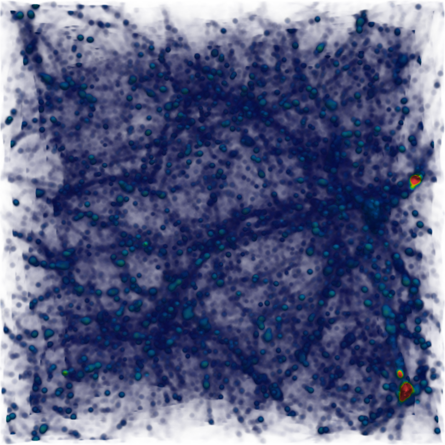
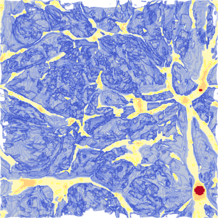
Figure 1: The DTFE density rendering (on the left) and the corresponding NEXUS+ Cosmic Web map (on the right). The two panels show the coco/color box with $70.4\times 70.4h^{-1}\,{\rm Mpc}$ on a side with a perspective z-direction mapping. The density is rendered so the below average density regions (all cosmic voids and some walls) are transparent. The corresponding Cosmic Web map on the right is rendered by setting all void regions to be fully transparent and the cosmic walls (i.e. void boundaries) are displayed in a tomographic projection with light shadows on a blue surface. On the near face of the simulation volume we see cross-sections through the nodes in red, filaments in orange and the walls in yellow. The nodes and filaments cannot be seen at farther distances since they are surrounded by thin wall regions.

We use the NEXUS+ algorithm (Cautun2013, ) for the segmentation of the Cosmic Web into its distinct morphological components: nodes, filaments, walls and voids. This method is an improved version of the MultiScale Morphology Filter (AragonCalvo2007, ) and includes more physically motivated prescriptions for determining the web environments. We chose this method due to its multiscale and parameter free character that make it an ideal tool for identifying in a robust manner the cosmic environments. Due to its scale-space approach, this method is equally sensitive in the detection of both prominent and tenuous filaments and walls. The tenuous environments are especially important to obtains a complete census of web environments for the faintest galaxies (i.e. lowest mass halos), since many of them are found in tendrils criss-crossing the underdense regions (Cautun2014, ; Alpaslan2014, ).

The NEXUS+ algorithm takes as input the DM density field on a regular grid. To take full advantage of the multitude of structures resolved by the COLOR simulation, we use the Delaunay Tessellation Field Estimator (DTFE) (Schaap2000, ; Weygaert2009, ) to interpolate the density to a $640^{3}$ grid corresponding to a $0.11h^{-1}\,{\rm Mpc}$ grid spacing. NEXUS+ starts by smoothing the input density field on a suite of scales from $0.125$ to $2h^{-1}\,{\rm Mpc}$. For this, it uses the Log-density filter, which corresponds to a Gaussian smoothing of the logarithm of the density field (Cautun2013, ). For each smoothing scale, the resulting density is used to calculate the Hessian matrix and its three eigenvalues. The values and signs of the eigenvalues are used to determine the environment response at each location, i.e. grid cell. The actual expression is rather involved (see Cautun2013 ), but qualitatively a region is classified as a filament if the two largest eigenvalues are negative (i.e. indicate collapse around those directions) and if their absolute values are much larger than the third eigenvalue. Then, at each location the results of all smoothing scales are combined by taking the maximum of all the values. This is because a web structure of a given thickness has its largest web signature when smoothing with a filter of the same width. Finally, the nodes, filaments, and walls are identified as all the grid cells whose environment response is above a self-determined threshold value (see Cautun2013 for details). The remaining volume elements that are not associated to nodes, filaments, or walls, are classified as part of voids. Our final Cosmic Web map consists of $256^{3}$ cells (i.e. $275h^{-1}\,{\rm kpc}$ grid spacing) where each cell is assigned one of the four web environments.

The NEXUS+ web environments are uniquely and robustly defined for an input density filed. The algorithm assigns to a given region of space the flag of an environment that has the strongest response function over a set of smoothing scales. It has been shown (Cautun2013, ) that the resulting environment classifications goes beyond a simple local-density mapping, and is sensitive to a multi-scale hierarchical nature of the Cosmic-Web. Because of this feature, the NEXUS+ environments only partially can be characterised by their density distribution functions, and the resulting PDFs are largerly overlapping (see Fig. 4 in Libeskind2018, ).

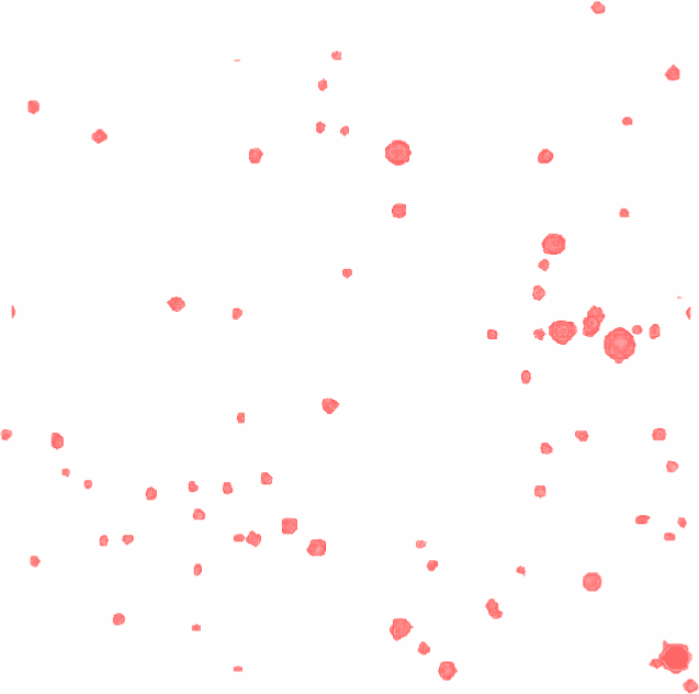
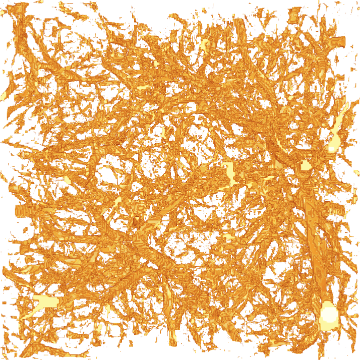
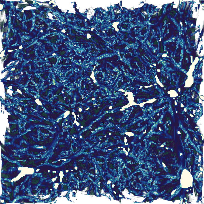
Figure 2: The coco/color volume NEXUS+ maps showing nodes (the upper-left panel), filaments (the upper-right) and walls (the bottom panel). The magnificent level of detail with which we recover the Cosmic Web is a result of the very high resolution of the coco/color suite.

IV Results

In what follows we present and discuss our main results. We use three different estimators to measure our sample statistical uncertainties. Where simple number counts dominate the statistics like in cases such as the mass functions estimations, we use the standard Poisson error. Whenever we estimate trends or functions of the data, we use bootstrapping to measure the uncertainty associated to the mean and median values for each bin. Finally, sometimes we study the spread or width of a distribution, which we quantify using $16^{\prime}$th and $86^{\prime}$th percentiles. We use percentiles instead of the usual standard dispersion since some of our data has non-Gaussian distributions and the standard deviation in that case could be misleading.

In FIG. 1 the DTFE density together with the corresponding NEXUS+ environmental map is shown. While the DTFE density field is continuous and is displayed using a projection rendering, the Cosmic Web map is a discrete tessellation of the simulation space and is represented in a tomographic projection. For the density field projection we set all regions with density less then the cosmic mean (i.e. $\delta<1$) to be transparent, which reveals the prominent network of filaments and nodes. We can also distinguish a number of spherical, ball-like regions, spread-out across the filamentary network. These indicate the prospective location of massive dark matter halos. The three green-red regions close to the right-hand density map boundary are nodes with surrounding thick filaments close to the projection plane.

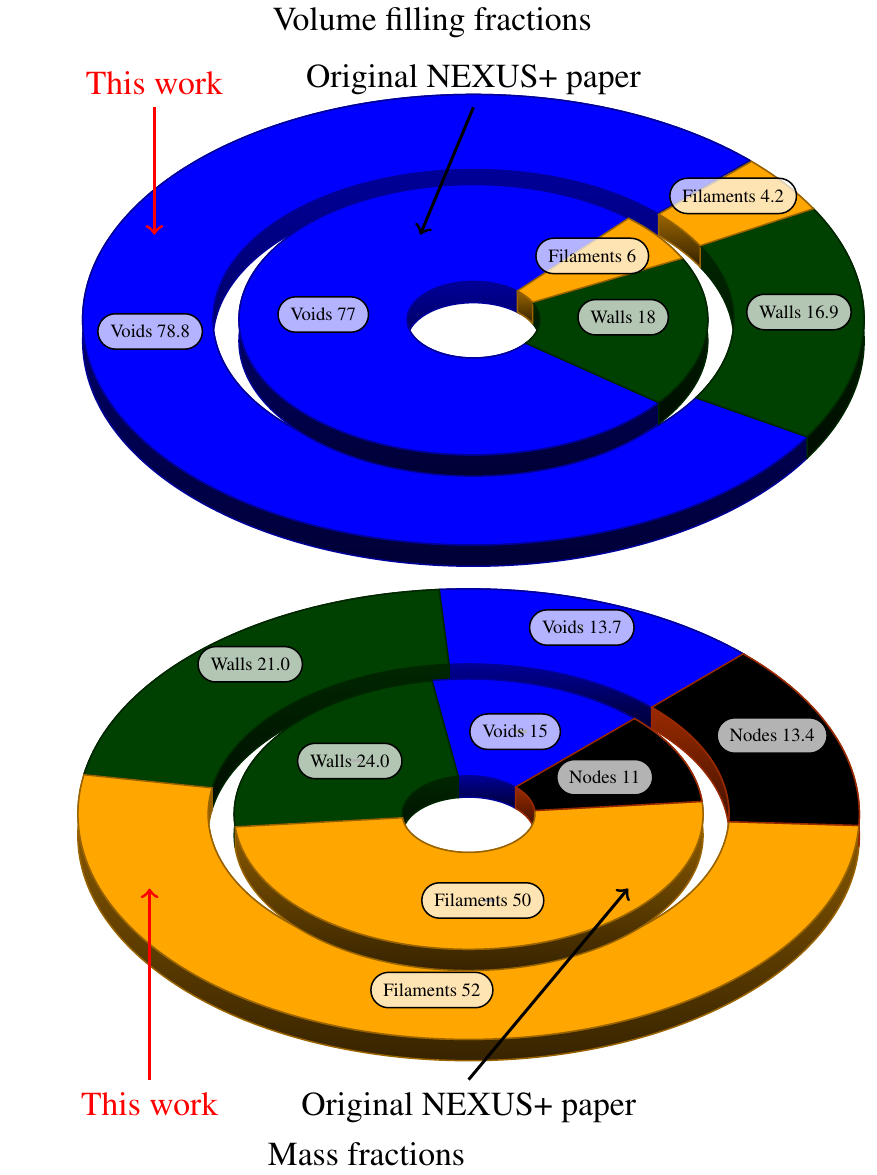
Figure 3: The Cosmic Web components in the coco/color simulation. The upper panel: The volume filling fraction of voids (blue), walls (Green) and filament (yellow). The volume fraction of the node environment, $0.045\%$, is so tiny that is is not displayed. The bottom panel: The fraction of the total mass found in each Cosmic Web environment. Here the nodes, denoted by orange, constitute a significant fraction of the mass.

The corresponding Cosmic Web segmentation shown in the right panel of FIG. 1 reveals a complicated inter-connected network full of small-scale details on the cosmic walls surfaces encompassing voids. The tomographic projection is not optimal to show the filamentary network because most filaments are surrounded by a thin wall-like environment. To allow for a clearer visualization of the various web environments, we plot the nodes, filaments and walls in three separate panels in FIG. 2.

We summarize the detailed segmentation studied here by illustrating the volume and mass-filling fractions of each Cosmic Web environment identified in color. This is depicted in Fig. 3. We can compare our results (outer ring) with the reference NEXUS results of Ref. Cautun2014 , which were obtained using the lower resolution Millennium simulations MS ; MS2 . We find good agreement, which is indicative of the fact that the color volume, while being smaller than the Millennium simulation one, it is still representative of the large-scale distribution of matter. The main difference is that while our filaments occupy slightly less volume they contain a somewhat higher mass fraction than the Ref. Cautun2014 filaments. This effect is due to the higher resolution of the color simulation, which allows for a better identification of the edges of thick filaments, hence the lower volume, and for the recovery of tenuous filaments that criss-cross the underdense regions, which lead to a somewhat higher mass fraction.

IV.1 Halo mass functions

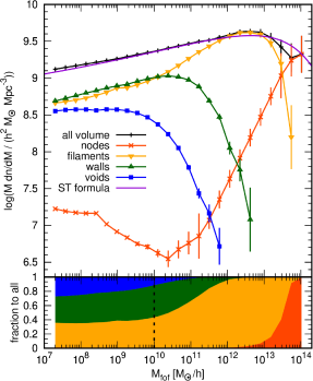
Figure 4: coco+color  halo mass functions for different environments. Upper panel: The FOF mass functions for $z=0$. The black line with crosses is the result for the whole volume, orange line with x-es depicts halos found in nodes, yellow with down-triangles is for filaments, green with up-triangles marks halos in cosmic walls and finally blue line with boxes shows void halo mass function. The solid magenta line illustrates the Sheth-Tormen prediction. The vertical bars indicate Poisson error-bars. Bottom panel: The fractions of FOF halos found in each specific environment. Lines show ratios of FOF mass functions in each environment w.r.t. the whole unsegmented simulation volume. The dashed vertical line marks the mass resolution limit of the original NEXUS+ papers (Cautun2013, ; Cautun2014, ).

A fundamental characteristic of any population of halos is their mass function, often refereed to as the halo mass Function (HMF). The HMF is simply a comoving number density of halos expressed as a function of their mass. The Cold Dark Matter (CDM) models predict that HMF has an exponential cut-off at large masses (i.e. cluster scales) and is characterized by a power-law, $\textrm{d}n/\textrm{d}M\sim M^{-\alpha}$, at small halo masses, with a slope $\alpha\sim 1$. This is due to a nearly scale-invariant power spectrum of the primordial density fluctuations and hierarchical nature of the structure formation process of CDM models (Press-Schechter, ; NFW2, ).

The results of excursion-set modeling based on spherical collapse of the formation of halos, which builds upon the Press-Schechter formalism(Press-Schechter, ), suggests that the HMF has an universal character when expressed in the terms of the root mean square variance of matter fluctuations, $\sigma(M,z)$, at given mass scale $M$ and redshift $z$. The predictions of Press-Schechter formalism further improved by ellipsoidal-collapse models (ShethTormen2002, ; Corasaniti2011b, ) (i.e. models relaxing the assumed sphericity of all halos) and has been a subject of intensive study and scrutiny in the past few decades (Tinker2008, ; Desjacques2008, ; Maggiore2010, ; Corasaniti2011, ). The literature about the halo mass function is very rich, which reflects its pivotal role in cosmology. The comoving number density of dark matter halos, as described by the HMF, is not directly observable, but it is a crucial ingredient in modeling many statistics and observables of crucial importance in cosmology. Precise HMF is needed in semi-analytical galaxy formation models (SAMSCole2000, ; Mtrees1, ), in the halo-model of the non-linear matter power spectrum, galaxy clustering predictions, weak-lensing shear and convergence observations, high-redshift Lyman-$\alpha$ 1D power spectrum and many others (e.g.  see Cooray2002, ; Conroy2006, ; SKibba2009, ; Reid2012, ).

The HMF was also studied in relation to the Cosmic Web, with most results pointing toward a picture, where fractions of halos forming and residing in different LSS environments varies as a function of their mass (see e.g. Alonso2015, ). Thus, one can decompose the overall HMF into different components representing the contribution of specific environments. Hence, as a starting point of our analysis, we study the halo mass function and its decomposition into the four components of the LSS as identified by the NEXUS+ method. The coco run has a relatively small volume and by selection does not contain any cluster-mass halos. This result in a relative scarcity of massive halos (i.e. $M\geq 10^{12}h^{-1}{\rm M}_{\odot}$) when compared to the expected universal mean. For that reason, to avoid any limited volume and density-related biases we choose to use the HMFs from the regular color box in the mass regime $3\times 10^{8}h^{-1}{\rm M}_{\odot}\leq M_{FOF}\leq 10^{14}h^{-1}{\rm M}_{\odot}$ and supplement it by the coco sample only at the low-mass $\stackrel{{\scriptstyle<}}{{{}_{\sim}}}3\times 10^{8}h^{-1}{\rm M}_{\odot}$, where color results are affected by resolution.

In FIG. 4 we show two panels that illustrate how the HMF in the coco+color sample depends on the Cosmic Web environment. The upper-panel shows the comoving HMF for all simulation volume, its segmentation into specific environments and, the Sheth-Tormen prediction (ShethTormen2002, ) obtained for the relevant set of cosmological parameters. Here, we use Friends-of-Friends as a halo mass, $M_{FOF}$, to allow a comparison with the previously published coco results. The lower-panel illustrates the fraction of halos found in each of the LSS environments in a given mass bin. The environmental HMF presented in this way enjoys a few interesting features. First, all of them, except for the nodes, exhibit exponential cut-offs at the high-mass end. These cut-offs are somewhat similar to the same feature of the all-volume halo mass, but they appear (i) sharper and (ii) manifest themselves at lower mass, and this mass is a specific function of the environment.

The void HMF has the smoothest cut-off and it is starting to plummet at $M_{FOF}\sim 10^{10}h^{-1}{\rm M}_{\odot}$, the abundance of wall halos is declining a bit sharper, and this takes place at nearly two decades higher mass of $\sim 10^{12}h^{-1}{\rm M}_{\odot}$ and finally the filament HMF is the one with the sharpest cut-off appearing at $M\sim\times 10^{13}h^{-1}{\rm M}_{\odot}$. The qualitative behaviour of our environmentally-segregated HMF agrees for $M\geq 10^{10}h^{-1}{\rm M}_{\odot}$ with the original NEXUS+ paper results. However, here thanks to our combined coco+color samples we are able to study for the first time the HMF of web environments below this mass. The fractions of small-mass halos residing in each of the tree main environments follow the trends hinted at higher masses, with the filament ratio gradually falling and the void ratio gaining at its expense. However, two observations are quite outstanding in this picture. First, we note that starting from masses $\stackrel{{\scriptstyle<}}{{{}_{\sim}}}5\times 10^{9}h^{-1}{\rm M}_{\odot}$ the wall and filament ratios roughly equalise and then they gradually decrease together in the favor of the void environment. Secondly, at our low mass-end, $M{\sim}2\times 10^{7}h^{-1}{\rm M}_{\odot}$, the division of halos among the three environments approaches an equal ratio of $1/3$rd for each. This will have significant repercussion, as we will see later, since the internal properties of halos in each of the environments do differ noticeably at those small masses. We need to be cautious of numerical effects close to the minimum coco halo mass for our study, which here is $M_{min}=100\times m_{p}^{COCO}=1.145\times 10^{7}h^{-1}{\rm M}_{\odot}$. The study of Ludlow_conv2019 , as well as the original coco simulation paper indicate that at this limit, the $M_{FOF}$ HMF is converged to within $5\%$, while $M_{200}$ based HMF converges to $<10\%$. The fractional contributions seen in FIG. 4 are however much larger than the uncertainty due to limited resolution, and thus unlikely to be significantly impacted by numerical effects.

The fact that our results suggests that at sufficiently low halo masses the fraction of halos found in voids, walls, and filaments becomes comparable and tentatively suggest an even partition of 1/3 in each of the three environments, reflect the superior resolution of the coco simulation. This allowed for the identification of the Cosmic Web environments in voxels of side-length of only $275h^{-1}\,{\rm kpc}$. At this level of details, the rich internal substructure of the Cosmic Web is revealed, and we can identify the filamentary tendrils and the tenuous walls that criss-cross voids and divide them into sub-voids.

An important question in the field is to what extent the variation of the HMF with the web morphology is driven by the change in density between environments. It seems that when defining the environment on large, $\sim 10h^{-1}\,{\rm Mpc}$, scales the HMF is mostly determined by the density (e.g. Alonso2015, ). However, the likely environment relevant for halo growth is the one on scales similar to the Lagrangian patch from which an object formed. When studying these scales, the anisotropies of the tidal field seemed to be more important with studies (Borzyszkowski2014, ; Paranjape2018, ; Ramakrishnan2019, ) showing that the anisotropy, and not the density, is the main driver of halo assembly bias. The multiscale nature of NEXUS+ allows it to adaptively determine the local scale on which the web is most pronounced and thus to capture the tidal field anisotropy on the relevant scale. The fact that vastly different mass fractions and volume fractions of each environments conspire to give comparable fraction of small-mass halos living in each of them is both interesting and surprising. These merit further and deeper investigation which, however, is beyond the scope of the current paper and we postpone it for future work.

IV.2 Density profiles

We have shown already that at sufficiently small masses (i.e. $\stackrel{{\scriptstyle<}}{{{}_{\sim}}}10^{10}h^{-1}{\rm M}_{\odot}$) the dark matter halo population segments into three environmental components, with significant fractions of halos locked in walls ($\stackrel{{\scriptstyle<}}{{{}_{\sim}}}35\%$), voids ($\stackrel{{\scriptstyle>}}{{{}_{\sim}}}25\%$) and filaments ($\stackrel{{\scriptstyle<}}{{{}_{\sim}}}35\%$). Now, we will investigate how the various web components affect the internal properties of their inhabiting halos. More precisely, we will compare averages over halo populations divided into each environments binned as a function of their $M_{200}$ mass.

Our main focus now is on the halo density profiles. Understanding their average trends with mass and evolution with time is of major importance for modern cosmology. We shall describe the halo density profile using the universal Navarro-Frenk-White (NFW) profile (NFW1, ; NFW2, ), which has been shown to be a reasonably good description of spherically averaged halo mass distribution for the majority of DM halos (but see also e.g. Neto2007, ; Ludlow2016, ; Wang2020, ). We use the NFW profile parameterized as

$${\rho(r)\over\rho_{c}}={\delta_{c}\over{r/r_{s}(1+r/r_{s})^{2}}}\,,$$ (1)

where $\rho(r)$ is the halo density averaged in a spherical shell of radius $r$, $\rho_{c}$ is the critical density of a flat universe, $\delta_{c}$ is the halo inner characteristic overdensity and $r_{s}$ is the so-called scaling radius. A standard approach that simplifies the analysis of the halo profiles is to define the concentration, $c_{200}$, parameter, expressed as:

$$c_{200}={r_{200}\over r_{s}}\,.$$ (2)

With the concentration parameter defined, the NFW profile effectively becomes a one parameter fit. This is becasue, the characteristic overdensity can be now expressed as:

$$\delta_{c}={200\over 3}{c_{200}^{3}\over{\rm ln}\,(1+c_{200})-c_{200}/(1+c_{200})}\,.$$ (3)

The NFW scale radius, $r_{s}$, gives the radial position at which the $r^{2}\rho(r)$ curve attains its maximum, which sometimes is also denoted by $r_{-2}\equiv r_{s}$. For the majority of DM halos, the peak of the $r^{2}\rho(r)$ curve is relatively broad. This means that, for halos resolved with a relatively small number of particles, the exact location $r_{-2}$ of the peak is subject to significant uncertainties due to the presence of noise. This, however can be significantly reduced when one works with stacked density profiles.

In our analysis we are interested to study $c_{200}$ for our halo populations split across different Cosmic Web environments. To get this we fit the NFW profile to all the halos with at least $N^{min}_{p}=1200$ particles for both coco and color samples separately. This yields $M^{min}_{200}=1.6\times 10^{8}$ and $7.4\times 10^{9}h^{-1}{\rm M}_{\odot}$ for coco and color simulations, respectively. For the specific discussion of the fitting procedure we refer the reader to the original simulation paper (COCO1, ).

Finally, as already mentioned the NFW profile is a good fit for objects that are close to dynamical equilibrium. Halos affected by recent major mergers or close encounters usually are not in equilibrium and the NFW functional form is not a good fit to their mass profiles. As a consequence, the concentration parameter derived from fitting non-relaxed halos is ill defined and at best biased low (see e.g. Neto2007, ; CMGao2008, ; Ludlow2010, ). To overcome this problem, we remove non-virialized halos, i.e. objects that do not jointly satisfy the following three criteria (Neto2007, ):

1. the fraction of halo mass contained in its resolved substructure is $f_{sub}<0.1$,

2. the displacement between the center of mass and the minimum of the gravitational potential cannot exceed $7\%$ of halo’s virial radius, $r_{200}$,

3. we require that the adjusted virial ratio $K_{vir}\equiv(2T-E_{s})/|U|$, is $K_{vir}<1.35$.

Here $T$ and $U$ are the halo’s total kinetic and potential energy and we include the Chandrasekhar’s pressure term, $E_{s}$, which quantifies the degree to which a given halo interacts with its surroundings. See Shaw2005 and their eqn. (6) for the definition and method used to estimate the pressure term, and also see Power2012 for a more detailed discussion about the virial ratio of halos. After applying the criteria described above, we have found that $\sim 21\%$ of the coco halos and $\sim 13\%$ of the color halos (for all mass range) are not relaxed and were removed from further analysis.

In FIG. 5 we show the median concentration-mass relation, $c_{200}(M_{200})$, for coco+color halos divided into different samples. We consider all-volume (black line), nodes halos (orange crosses and lines), filaments halos (yellow down-triangles and lines), walls halos (green up-triangles and lines) and halo found in voids (blue squares and lines). For a comparison we show also the prediction of Ref.(Ludlow2016, ) model as a purple solid line. The error bars reflect the uncertainty with which we can calculate the median in each bin, which was obtained using 100 bootstrap samples, while the shaded region illustrates the halo-to-halo spread, which is the 16-th and 86-th percentile of the halo population in each mass bin (it corresponds to the $1\sigma$ variance for a normally distributed random variable).

We notice that the modeled $c(M)$ relation of Ref.(Ludlow2016, ) describes well the trend exhibit by the main all-volume sample. The things become interesting when we study the behavior of the samples belonging to different Cosmic Web segments. Here, it seems that the nodes-halos are described by starkly higher median concentrations than the overall population, and, moreover, for objects with $M_{200}\stackrel{{\scriptstyle<}}{{{}_{\sim}}}10^{12}h^{-1}{\rm M}_{\odot}$ the $c(M)$ relation appears to be much flatter than what we can observe for the other samples. The remaining LSS environments follow closely the main sample trend, with some appreciable scatter. This, however, applies only to halos more massive than $M_{200}\sim 10^{11}h^{-1}{\rm M}_{\odot}$. For lower-mass objects the median concentrations in each web environment start to deviate systematically from the all-volume median. Here, the void halos appear to be characterized by density profiles with lower concentrations than the universal sample, while the filaments halos, on the other hand, have higher concentrations. Deviations of both samples seem to increase with decreasing halo mass. Interestingly, the wall sample is characterized by the concentration-mass relation that is very close to the universal sample. To better understand and quantify the trends with halo mass and environment, we fit the $c(M)$ relation for each environment with a broken power-law of the form:

$$c_{200}(M_{200})=\begin{cases}A(M_{200}/M_{th})^{b_{l}}&\text{for}\,\,M_{200}\leq M_{th}\\ A(M_{200}/M_{th})^{b_{h}}&\text{for}\,\,M_{200}>M_{th}\end{cases}$$ (4)

Table 1: The best-fitting $c_{200}(M_{200})$ parameters to the double power-law of Eqn. (4) for all the data samples shown in FIG. 5. $M_{th}$ is expressed in $\times 10^{10}h^{-1}{\rm M}_{\odot}$, while max mass is in $h^{-1}{\rm M}_{\odot}$.

Sample	$A$	$M_{th}$	$b_{l}$	$b_{h}$	max mass
All-volume	9.89	6.12	-0.057	-0.092	$10^{14}$
nodes	16.9	114	-0.013	-0.313	$10^{14}$
filaments	9.97	6.12	-0.076	-0.092	$10^{14}$
walls	9.59	6.12	-0.063	-0.077	$3\times 10^{12}$
voids	9.72	6.12	-0.046	-0.092	$6\times 10^{11}$

The single power-laws were used to described various $c(M)$ and has been shown to characterize reasonably well halos from various simulations, albeit only for a limited mass range (Neto2007, ; CMGao2008, ; Ludlow2010, ; Klypin2011, ; Munoz2011, ; Prada2012, ; Sanchez-Conde2014, ). We use double power-law for our samples, since it appears that there is a close to universal mass-scale at which the various Cosmic Web populations deviate from the mean trend describing the overall halo population. In Eqn. (4) the mass scale at which the broken-law changes the slope is defined as $M_{th}$, while $A$ is the normalization factor, $b_{l}$ and $b_{h}$ are the (l)ow and (h)igh-mass power-law slopes. We have found that the double power-law of the above form offers very good fits to all our data-samples. We have collected parameters for all the samples in Tab. 1. All fits have the same minimal mass of applicability set to $10^{8}h^{-1}{\rm M}_{\odot}$, the corresponding maximal masses are given in the table.

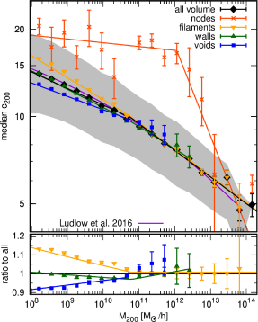
Figure 5: coco+color concentration-mass relation split across the different Cosmic Web environments. The Upper Panel: The $c(M_{200})$ relations for our joint samples. The data points and error-bars represent the median and its bootstrap error from the simulation data. The solid lines with matching color are the best-fitting broken power-laws (see the main text). The shaded region illustrates the 16-th:84-th percentiles for the all-volume sample. The purple line shows the prediction of Ludlow et al. 2016 model. The Lower Panel: The relative ratio of the data and the fits for void, walls and filament halos taken with respect to the all-volume sample.

For the void sample, we could not robustly determine $b_{h}$, i.e. the power-law slope for the high-mass regime, since there are only a handful of halos with $M_{200}>M_{th}$ found in voids. Because of this the variance of halo concentrations in that mass regime is considerably high, and in turn the whole void halo population can be well described by a single power-law. Nonetheless, the void-sample still can be described very well by a double power-law, by using the $b_{h}$ value measured for the all-volume sample. The analysis of the best-fit parameters that describe our halo samples highlights a couple of very interesting features.

Firstly, we find that the population of halos found in node environments is very different from the rest of the sample. Up to threshold mass of $M^{node}_{th}=1.14\times 10^{12}h^{-1}{\rm M}_{\odot}$ their concentration-mass relation is relatively flat, slowly dropping with halo mass, with the power-law slope of $b_{l}=-0.13$. Above this mass, the node sample experience a dramatic shift to a steeply declining power-law with slope of $b_{h}=-0.313$. This can be understood when we realize that the majority of small-mass halos found in nodes are actually satellite halos found usually just outside the viral radii of much more massive halos found at the nodes of the Cosmic Web. Potentially many of them may be the so-called backsplashed halos, which traversed one or more times through the virial radius of a larger halo (Behroozi2014, ; Adhikari2014, ; Busch2017, ; Diemer2020, ). Therefore, these low-mass objects, although officially classified as distinct halos, can be to some extent subjects to preprocessing such as: tidal truncation, stirring and disruption, just as regular subhalos found within the virial radius of their host halos. Above the $M_{th}$ the node sample starts to be dominated by regular halos. This is also indicated by the growing fraction of halos found in nodes in that mass range (see again Fig. 4). It explains why the $c(M)$ experiences such a steep decline to arrive again at the universal all-volume median for $M_{200}\stackrel{{\scriptstyle>}}{{{}_{\sim}}}10^{13}h^{-1}{\rm M}_{\odot}$.

The three remaining Cosmic Web elements paint a more coherent picture. Here, all three samples approach the all-volume universal mean for the same threshold mass of $M_{th}=6.12\times 10^{10}h^{-1}{\rm M}_{\odot}$. Although, we find slightly different best fitting values for $b_{h}$, i.e. the high-mass slope of the $c(M)$ relation, the relation can be reasonably well described also by the all-volume high-mass fit. This specific threshold mass was surprisingly universal across the different Cosmic Web segments and what is even more important, we find it to also has the same value when analysing the coco and color samples separately. Below the threshold mass we observe clear departure of the distinct samples from the all-volume median. Here, the void halos density profiles get less and less concentrated compared to the universal mean, while the filament halos are characterized by denser central density profiles. Strikingly, the wall halo population appears to have the median concentration parameter that most closely follows the all-volume sample. This would indicate, that the wall halos find themselves in a perfect balance between higher-density filaments and empty voids to arrive at a median that is very close to the overall value. The maximum deviation between different populations is observed at $M_{200}=10^{8}h^{-1}{\rm M}_{\odot}$, where the median $c_{200}$ of the filament sample is higher by $\sim 15\%$ then the overall population. Here the median void halo concentration is $\sim 8\%$ lower compared to the all-volume sample. For halos with one order of magnitude higher masses these discrepancies shrink to $8$ and $6\%$ respectively. Finally at masses $\stackrel{{\scriptstyle>}}{{{}_{\sim}}}10^{10}h^{-1}{\rm M}_{\odot}$ the three Cosmic Web samples start to quickly converge towards the overall trend.

Our data do not allow to accurately study profiles below a halo mass of $\sim 10^{8}h^{-1}{\rm M}_{\odot}$, so we are unable to check if the environmental trends would continue. However, there is a hint in our data, seen both for voids and filaments, that the deviation from the all-volume median starts to flatten at masses of $\sim 4\times 10^{8}h^{-1}{\rm M}_{\odot}$. This can be seen for the two least massive bins in FIG. 5. If this would be indeed the case, then a more natural scenario would be favoured, where the environmental effects on the halo concentrations are, at best, saturating at around our maximal deviations, rather than growing further with decreasing mass. Thus, we need to caution against extrapolating the trends exhibited by our best-fits to lower halo masses.

Recently, in a work dedicated to study halo concentration over 20 decades in mass, (Wang2020, ) claimed that the halo concentrations are insensitive to “the local halo environment”. Our results would then seem to be in conflict with theirs. However, we note that the Ref.(Wang2020, ) use a rather specific definition of a halo environment. First, they consider only the local density, as measured in a sphere around a halo. Second, the density used for this specific proxy of a halo environment is measured on a scale $5-10\times R_{200}$. Thus it is a scale-dependent density measure. In contrast, the NEXUS+ environment is defined on scales that maximises the Hessian response signal, depicting and reflecting the multi-scale nature of the Cosmic Web (see more in Cautun2014, ). In fact, there is no correlation between our Cosmic Web flags and the local-density measure used by Ref.(Wang2020, ). In addition, what plays here an important role is the fact that the Ref.(Wang2020, ) used a series of nested zoom-in simulations, which begins with a parent region of a relatively low density. Thus, starting from their level-2 (L2) zoom their halo population, according to the definitions and criteria used in this work, would belong to only one specific NEXUS+ environment. Since they place each nested consecutive zoom-in region far away from massive halos, would most likely favour NEXUS+ wall or void environments. It would be interesting to see, if the environmental trends we have found hold down to lower halo masses. Such a study will require a separated dedicated set of zoom-in simulations, similar to the ones employed by Ref.(Wang2020, ) and we leave this aspect for future work.

Whether the mass threshold of $M_{th}=6.12\times 10^{10}h^{-1}{\rm M}_{\odot}$ is a universal parameter related to the $\Lambda{\rm CDM}{}$ Universe and the NEXUS+ method is a subject of an open debate. We can suspect that this new mass scale might be a function of the background cosmology, but other factors like the impact of a simulation volume or mass resolution cannot be excluded at this time. A more detailed study that would involve usage of many different N-body simulations would be required to address this question. We leave such a study for the future. However, the implications of the existence of $M_{th}$ below which the universality of the concentration-mass relation is broken, might be profound. Especially, when we recall that below this mass scale the fraction of halos inhabiting each of the three different environments is significant and approach an equal division. We will discuss the consequences of this result in the concluding section.

IV.3 Mass assembly histories

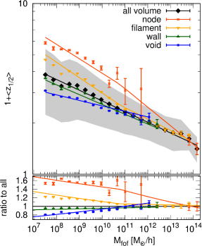
Figure 6: The average coco+color formation redshifts, $\langle z_{1/2}\rangle$, for halos split according to their web environment. The Upper Panel: The halo formation redshifts plotted versus $z=0$ FOF halo mass. The points with error bars correspond to our simulation data, while the solid lines are the best fitting relations (see the main text). The shaded region marks the 68 percentiles for the all-volume sample. The error bars indicate bootstrap errors on the mean. The Lower Panel: The ratios of the formation redshift in the different environments with respect to the all-volume sample.

In the previous section we have found a clear effect of the different Cosmic Web environments on the median halo concentrations. In hierarchical structure formation cosmologies, such as the CDM model, halo concentrations are correlated with some characteristic halo formation times. This reflect the fact that due the hierarchical bottom-up build-up of the halos the inner-most regions of dark matter halos are the first one to be assembled. The material acreeted later has usually higher angular momenta, which means that it seldom is able to settle down in the central parts of the halo mass distribution. In such a picture the inner parts of the halo density profiles are dynamically old, and the density reached there during the assembly time sets the halo concentration. Since the averaged background density of the Universe drops with time, older halos have usually higher central density and also higher concentrations. For the $\Lambda{\rm CDM}$ model this scenario is evident in a wealth of simulations-based studies (Ludlow2010, ; Ludlow2016, ; Rey2019, ; WangKuan2020, ; Chen2020, ).

The clear correlation between the redshift of the halo assembly (also called the formation redshift) and the halo concentration suggest that we should also see the effect induced by different Cosmic Web environments in the halo assembly histories. For each halo, we define the formation redshift, $z_{1/2}$, as the redshift at which the most massive progenitor (MMP) of the halo reaches half of the final $z=0$ halo mass ((see Li2008, , for other possible definitions)). Thus, we define

$$M(z_{1/2})\equiv{\textstyle{1\over 2}}M(z=0)\,.$$ (5)

To find $z_{1/2}$ for the coco and color halos we follow the halo merger trees constructed as described in the section §II. Here, the mass of the MMP branch at each redshift is that of it’s parent FOF halo at that time. Next, we bin halos according to present-day $M_{FOF}$ and calculate the mean formation redshift, $\langle z_{1/2}\rangle$, in each bin and for each web environment. The obtained $z_{1/2}(M_{fof})$ relation is described by a linear fit in $\log(1+z_{1/2})$, same as in MS2 ; COCO1 , which takes the form:

$$1+\langle z_{1/2}\rangle=A_{half}\left({M_{FOF}\over M_{th}}\right)^{\beta_{half;\;1}}\,.$$ (6)

In previous studies, this power law was rescalled by a $10^{10}h^{-1}{\rm M}_{\odot}$ mass, however here we choose to use the characteristic environment threshold mass of $M_{th}=6.12\times 10^{10}h^{-1}{\rm M}_{\odot}$ found in the previous paragraph. Such a single power-law turned to be a good fit to the all-volume, wall and voids samples. For the filaments and nodes samples we had to use a two-regime power law

$$1+\langle z_{1/2}\rangle=\begin{cases}A_{half}\left({M_{FOF}\over M_{th}}\right)^{\beta_{half;\;1}}&\text{for}\,\,M_{FOF}\leq M_{th}\\ A_{half}\left({M_{FOF}\over M_{th}}\right)^{\beta_{half;\;2}}&\text{for}\,\,M_{FOF}>M_{th}\\ \end{cases}$$ (7)

with two power-law breaking mass scales set to be at the environment threshold mass $M_{th}$. We give the best-fit parameters of the averaged $1+\langle z_{1/2}\rangle$ relations for all our data samples in Tab. 2.

Table 2: The best-fitting parameters for the dependence of the halo formation redshift on halo mass. The dependence is given by the power-laws of Eqn. (6)-(7) and are shown in FIG. 6. The rows that do not have a value for $\beta_{form;\;2}$ mean that they were well fit by the single power-law given in Eqn. (6).

Sample name	$A_{form}$	$\beta_{form;\;1}$	$\beta_{form;\;2}$
All-volume	2.40	-0.063	–
nodes	3.35	-0.084	-0.109
filaments low	2.54	-0.09	-0.067
walls	2.31	-0.057	–
voids	2.37	-0.032	–

In FIG. 6 we plot the average formation redshifts, $1+\langle z_{1/2}\rangle$, and their associated best fits (the Upper Panel) for all halos and for halos in each web environment. To better highlight the trends, the bottom panel of the figure shows the relative difference with respect to the all-volume sample for our joined coco+color data. Despite the fact that some of the CW components (i.e. the nodes and filaments halos) experience a more complicated multi-slope relation, we clearly identify a common feature to the all data samples: a monotonic decline of the formation redshift with increasing halo mass. This reassures that in all the CW elements the halo build-up is still, as expected, progressing in a hierarchical manner. Comparing the different environments, we see that below the characteristic threshold mass $M_{th}=6.12\times 10^{10}h^{-1}{\rm M}_{\odot}$ the formation redshift at fixed halo mass depends on the CW component in which a halo is located. The voids halos have significantly lower $z_{1/2}$ compared to the all-sample mean, while on the other hand the filament population have higher formation time mirrored in a nearly prefect way to the void sample. The node FOF groups are the oldest in our runs, thus the NEXUS-node sample trace the first halos to form in the Universe. Here, the wall population has a value a bit lower than the assembly times for the whole population, however, the effect is small and contained to within $5\%$.

Similarly to the density profiles, the trend with environment becomes more and more prominent as we decrease the halo mass. What is also really noticeable is that the trend with the CW is at the same level as that seen for $c_{200}$, reaching a maximum $20\%$ difference for filament and void halos at $M_{FOF}=3\times 10^{7}h^{-1}{\rm M}_{\odot}$. It highlights how the local CW environment moderates the merger and accretion rates of halos that, in turn, is reflected in the halo formation times. The effect is only significant for halos less massive than a characteristic environmental mass scale, $M_{th}$.

IV.4 The $V_{\textrm{max}}$-$R_{\textrm{max}}$ relations

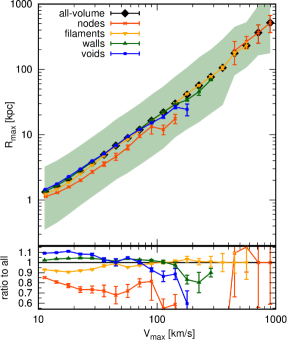
Figure 7: The median coco+color $R_{\textrm{max}}-V_{\textrm{max}}$ relation for halos in different Cosmic Web structures. The Upper Panel: $R_{\textrm{max}}-V_{\textrm{max}}$ for all samples. The errors on the data points reflect the bootstrap errors on the medians. The shaded green region marks the 15-th to 84-th percentile spread around the all-volume sample. The Lower Panel: The relative ratio of each Cosmic Web population to the all-volume sample.

Another complementary probe of the halo mass distribution is the shape of the circular velocity curve, which due to its cumulative nature is less prone to small density fluctuations due to, e.g. substructures, as is the case for the differential measure of $\rho(r)$. The circular velocity is defined as:

$$V_{c}(r)=\sqrt{{\textrm{G}M(<r)\over r}}\,,$$ (8)

where $M(<r)$ is the mass enclosed inside a sphere of radius $r$ centred at the halo centre. For a halo that exhibits perfect spherical symmetry, the circular velocity, $V_{c}(r)$, is exactly equal to the circular orbital velocity at distance $r$. For well resolved and relaxed halos, the circular velocity takes only one maximum value, $V_{\textrm{max}}$, that occurs at a radial distance, $R_{\textrm{max}}$. Now, studying the $V_{\textrm{max}}-R_{\textrm{max}}$ relation gives a way to characterize the halo internal mass profile, based on its internal dynamics. The $M(<r)$ profile is simply a linear convolution of the halo density profile. Thus in principle, the information contained by the $V_{\textrm{max}}-R_{\textrm{max}}$ is the same as the one encoded in halo density profiles. However, the dynamical measure of $V_{\textrm{max}}$ is, in principle, easier to access by observations than the measurement of the halo concentration profile, which is why we perform a separate analysis of the $V_{\textrm{max}}-R_{\textrm{max}}$ relation.

Here we investigate the $V_{\textrm{max}}-R_{\textrm{max}}$ relation for our joint main halo samples. Generally we can expect that the smaller $R_{\textrm{max}}$ at fixed $V_{\textrm{max}}$ the steeper the inner $M(<R)$ profile. Indicating a halo with a denser inner region and by logic a higher concentration parameter. However, due to the cumulative nature of the $M(<R)$ distribution the $V_{\textrm{max}}-R_{\textrm{max}}$ relation is more stable against shot-noise. We will use this property to check and probe the environmental effects down to halos even smaller (i.e. $V_{\textrm{max}}=10\,{\rm km}\,{\rm s}^{-1}$) than this was possible for $\rho(r)$.

We start by constructing the joined color+coco sample, this time we consider all coco  halos down to $V_{\textrm{max}}=10\,{\rm km}\,{\rm s}^{-1}$, which is the convergence limit for $V_{\textrm{max}}$ for this run (see COCO1 for more detailed analysis). The color  population is susceptible to resolution effects at higher velocity values due to combination of lower mass, but also force resolution. Thus we set a lower-cut for color  halos at $V_{\textrm{max}}=40\,{\rm km}\,{\rm s}^{-1}$, and consider only halos above this threshold for our composite sample. Lastly, we use the Springel et al. (Springel2006, ) approach to correct the measured $V_{\textrm{max}}$ values for effects arising due to the force softening used in N-body gravity calculations, which consists of lowering the maximum velocity, $V_{\textrm{max}}$, of low-mass objects whose $R_{\textrm{max}}$ is comparable to the gravitational force softening of the simulation. We apply the correction formula proposed by (Aquarius, , Eqn. (10) therein), which, under assumed perfect circular orbits, accounts for this effect. After applying all the above steps we obtain a sample of $V_{\textrm{max}}-R_{\textrm{max}}$ pairs that robustly sample the maximum of circular velocity over three orders of magnitude, i.e. $10\leq V_{\textrm{max}}/(\,{\rm km}\,{\rm s}^{-1})\leq 1000$. The corresponding halo mass range then is from $2\times 10^{7}h^{-1}{\rm M}_{\odot}$ to $10^{14}h^{-1}{\rm M}_{\odot}$ (see e.g.Fig. A1 in COCO1 ).

In FIG. 7 we show the median $V_{\textrm{max}}-R_{\textrm{max}}$ relation for all our halo populations.The shaded green region illustrates the spread around the all-volume sample as measured by the 16-th and 84-th percentiles, which would correspond to $1\sigma$ dispersion for a Gaussian-distributed random variable. First, we find that the the spread has a nearly constant width (as measured using relative ratio) for the whole range of probed maximum circular velocities. Secondly, we see that region with $V_{\textrm{max}}\stackrel{{\scriptstyle<}}{{{}_{\sim}}}15\,{\rm km}\,{\rm s}^{-1}$ seems to be already affected to some extent by the resolution effects, which is indicated by the small, albeit noticeable, flattening of the relation. We opt to keep this data in the comparison, as we expect that this resolution effects would affect alike all Cosmic Web components. Henceforth the environmental signal encoded there is still useful, provided that for $V_{\textrm{max}}\stackrel{{\scriptstyle<}}{{{}_{\sim}}}15\,{\rm km}\,{\rm s}^{-1}$ we study only the relative ratios.

A number of interesting features visible in figure 7 deserve further attention. The effect of the Cosmic Web environment is also clearly visible here, and what is very reassuring the magnitude of $R_{\textrm{max}}$ reduction (boost) is consistent with the measured increase (reduction) of halo density concentrations seen in FIG. 5. This again, as we already seen it before, follows a nearly mirrored effects for voids and filament halos, reaching a maximum effect of $\sim 11\%$ for both environments at $V_{\textrm{max}}=18\,{\rm km}\,{\rm s}^{-1}$, which corresponds to halo mass of $\sim 4\times 10^{8}h^{-1}{\rm M}_{\odot}$. The net-effect of the environmentally-driven $V_{\textrm{max}}$ boost or reduction is a few percent-points smaller than what we observed for median $c_{200}$, however this is not surprising taking into account the fact that $V(R)$ is cumulative. What is very important is that using $V_{\textrm{max}}-R_{\textrm{max}}$ data we can now confirm the flattening (or saturation) of the Cosmic Web induced effect appearing for $M\stackrel{{\scriptstyle<}}{{{}_{\sim}}}4\times 10^{8}h^{-1}{\rm M}_{\odot}(V_{\textrm{max}}\stackrel{{\scriptstyle<}}{{{}_{\sim}}}20\,{\rm km}\,{\rm s}^{-1}$). Which was previously only hinted by our $c_{200}-M_{200}$ data. This result indicates that our fits for the environmental deviations from the universal $c(M)$ relation shown in Tab. 1 by no means should be extrapolated below the minimum $10^{8}h^{-1}{\rm M}_{\odot}$ mass. A more realistic modeling would seem to consists of a saturation of the difference, rather then the extrapolation of the trend seen at higher masses.

Another feature seen in our data is that, if we disregard the discrepancies between voids and walls samples for large objects (i.e.$V_{\textrm{max}}\geq 100\,{\rm km}\,{\rm s}^{-1}$) where the uncertainty is already high, we observe that the void, filament, and wall halos converge to all-volume value for $V_{\textrm{max}}\geq 80\,{\rm km}\,{\rm s}^{-1}$. This value of the maximum of the circular velocity curve corresponds to halo mass of $5-6\times 10^{10}h^{-1}{\rm M}_{\odot}$, a value very close to the universal environmental threshold mass, $M_{th}=6.12\times 10^{10}h^{-1}{\rm M}_{\odot}$, we found for the $c(M)$ and $z_{1/2}(M)$ relations. For the node halos the $V_{\textrm{max}}-R_{\textrm{max}}$ relation reveals a picture that is very consistent to what we have seen before. Only big and massive halos (in the galaxy group and cluster mass regime) follow the all-volume trend – this is expected by construction, since in this mass range the majority of halos live in the node environment. At lower masses, in the whole probed regime of $10\leq V_{\textrm{max}}$(s/km)$\leq 150\,{\rm km}\,{\rm s}^{-1}$ the node halos have smaller $R_{\textrm{max}}$ values at fixed $V_{\textrm{max}}$, which corresponds to more compact and concentrated density profiles. The reduction in $V_{\textrm{max}}$ is substantial and typically is of the order of $20$ to $30\%$ percent, when compared to the all-volume sample. The visible trend of increasing $R_{\textrm{max}}$ reduction when going from smaller to larger $V_{\textrm{max}}$ values is fully consistent with the relative flatness of $c(M)$ for nodes, since larger objects would have typically smaller concentrations, thus to obtain a nearly flat trend the decrease in $R_{\textrm{max}}$ needs to be larger.

IV.5 Shape and spin

So far we focused on the one primary halo internal property, namely its mass distribution. There are of course more properties intrinsic for each DM halo, that are of importance and interest. The other two that are commonly measured in simulations and used in a variety of modelling are the shape and spin parameters. The former is related to the symmetry of the internal mass distribution as traced by the halo mass inertia tensor, while the later is used as a measure of the net bulk internal rotation and is usually characterized using the halo angular momentum.

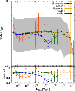
Figure 8: The median coco+color halo spin, $\lambda_{200}$, as a function of halo virial mass, $M_{200}$, and Cosmic Web environment. The Upper Panel: $\lambda_{200}(M_{200})$ relation for all samples. The errors on the data points reflect the bootstrap errors associated to the median calculation. The shaded gray region marks the 16-th:84-th percentile spread of the all-volume sample. The Lower Panel: The relative ratio for each Cosmic Web halo population with respect to the all-volume sample.

We first take a look at the halo degree of rotational support as measured by the halo spin parameter, $\lambda$. To calculate it, we use the Bullock definition (Bullock2001, )

$$\lambda={|j|\over{\sqrt{2}R_{200}V_{200}}}\,\,,$$ (9)

where $V_{200}$ is the value of the circular orbit velocity from Eqn. (8) taken at the virial radius $R_{200}$, and $j$ is the specific angular momentum of the halo

$$j={1\over N_{p}}\sum^{N_{p}}_{i}r_{i}\times v_{i}\,.$$ (10)

There are other definitions of this parameter (e.g.(Peebles1969, )), but the formulation from Ref.(Bullock2001, ) is one of the most convenient to measure from simulations. The spin parameter characterizes to what extent the halo is rotational supported. Halos with low spin are dominated by velocity dispersion of random motions and have low degree of overall rotation. On the other hand, we can expect that halos with high $\lambda$-s show more signs of coherent rotation in their orbital structure. The $\lambda$ parameter for $\Lambda{\rm CDM}{}$ cosmology has been studied in a number of previous works (e.g. Steinmetz1995, ; Cole1996, ; Maccio2007, ; Hellwing2013, ; Braun-Bates2017, ), and it has been generally found that DM halos are characterized by low spin values, consistent with a marginal degree of a coherent rotation. The distribution of the spin parameter has been found to be log-normal with the mean (i.e. the first moment) between $0.04-0.05$ at $z=0$ (e.g. Warren1992, ; Cole1996, ; Vitvitska2002, ; Bett2007, ). These log-normal mean values corresponds to median values in the $0.02\stackrel{{\scriptstyle<}}{{{}_{\sim}}}\lambda_{med}\stackrel{{\scriptstyle<}}{{{}_{\sim}}}0.04$ range. In FIG. 8 we show using our usual pattern of two panels the median virial spin parameter as measured at $R_{200}$ for halo samples split among different Cosmic Web elements.

The environmental effects in the spin parameter that we can see in the Figure follow much less obvious patterns than it was the case for the density profiles. Noticeably, here the effect of the environment appears to be present only for more massive halos, rather than for the lowest-mass objects like we have found in the previous section. The node-halo sample again has the largest uncertainties in the median value, and with our limited statistic it is hard to draw any firm conclusions. On the other hand, the effect seen in the void population is quite prominent and very interesting. Starting from $M_{200}\geq 3\times 10^{10}h^{-1}{\rm M}_{\odot}$ that sample experiences a growing departure from the universal all-volume trend. At $2-4\times 10^{11}h^{-1}{\rm M}_{\odot}$, which is the high-mass end of the void population, the reduction in $\langle{\lambda_{200}}\rangle$ reaches nearly $\sim 35\%$, which is quite a strong spin reduction. The most massive end of the wall population shows a hint of a similar trend, alas our statistics are too poor to confirm this in a robust way. Interestingly, for $M_{200}\leq 5\times 10^{11}h^{-1}{\rm M}_{\odot}$ the wall sample shows very small, yet consistent and significant excess of the spin with respect to the main sample. In contrast, the median spin of the filament halos of masses $10^{8}\leq M_{200}/(h^{-1}{\rm M}_{\odot})\leq 4\times 10^{9}$ is smaller by $\sim 5\%$ then the main sample.

There are different ways in which halos acquire non-vanishing total angular momentum. In the linear and weakly non-linear regime the spin is generated by torques induced by tidal fields associated with the local large-scale structure. This idea was first formulated as the Tidal-Torque-Theory (TTT) to explain the angular momentum of galaxies (Peebles1969, ; White1984, ; Barnes1987, ; Heavens1988, ; Catelan1996, ). The TTT explains well the growth of the angular momentum at early times. The insight from N-body simulation indicated that once the halo experience more rapid merger rates and mass accretion rate the primordial spin acquired via tidal torques becomes subdominant. This is because the specific angular momentum $j$ from Eqn. (10) is effectively a mass weighted quantity, as we use N-body particles as tracers. At later times the majority of halo particles consists of the material that resides in more outer-parts and their net angular momentum tends to be a bit higher reflecting both the increased radial distance and the non-linear character of halo mergers and late-stage of mass accretion (Porciani2002A, ; Porciani2002B, ; Robertson2006, ; Lopez2019, ). In this picture, halos that would live in a much less violent and crowded environment would naturally express a lower spin. This is exactly what our results for voids and walls populations indicate. A bit puzzling is what we observe for low mass node halos, which tend to have marginally significant lower spin then the all-volume sample. This merit a more thorough investigation, and we lave such for future work.

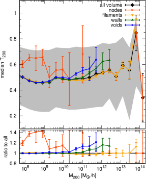
Figure 9: The coco+color median halo triaxiality shape parameter, $T_{200}$, as a function of halo mass, $M_{200}$. The Upper Panel: $T_{200}(M_{200})$ relation for all samples. The errors on the data points reflect the bootstrap errors around the medians. The shaded gray region marks the 16-th-84-th percentile spread around the all-volume sample. The Lower Panel: The relative ratio of each Cosmic Web population to the all-volume sample.

To measure the halo shape we use the eigenvalues of the halo’s mass tensor of all the particles within $\leq R_{vir}$ that do not belong to any substructure:

$$I_{ij}={{1}\over{N_{p}}}\sum_{N_{p}}x_{i}x_{j}\,\,,$$ (11)

where the particle positions $x_{i}$ and $x_{j}$ are with respect to the center of mass of the halo and the sum is over all the particles that belong to a given halo. The eigenvalues of this tensor corresponds to squares of the principal axes of the halo shape ellipsoid. We sort the eigenvalues and normalize them by the largest axis:

$$a>b>c\,,\quad\tilde{b}=b/a\,,\quad\tilde{c}=c/a\,,\quad\tilde{a}=1\,.$$ (12)

In general, we expect halos to be tri-axial ellipsoids that can be either prolate or oblate (e.g. Warren1992, ; Cole1996, ). The halo overall shape can be reasonably well described by a single parameter that is a combination of the all three eigenvalues. This is the halo triaxiality parameter

$$T_{200}\equiv{{a^{2}-b^{2}}\over{a^{2}-c^{2}}}={{1-\tilde{b}^{2}}\over{1-\tilde{c}^{2}}}\,.$$ (13)

Values of $T$ closer to unity indicate a shape that is closer to a prolate ellipsoid, in contrast low $T$ value corresponds to an oblate halo.

We study the median triaxality as a function of halo mass in FIG. 9, where two panels show the absolute values (the upper one) and the ratios with respect to the all-volume sample (the bottom panel). The gray shaded region shows the dispersion measured by the 16 to 84-th percentile spread around the median all-volume sample and the symbols with error bars indicate the uncertainties associated to the median calculation. The general trend visible for all environments except the nodes is consistent with a common picture emerging from N-body simulations. Namely, that more massive halos tend to be more prolate. This reflects their younger dynamical states compared to the less massive halos (Allgood2006, ; Bonamigo2015, ; Despali2017, ; Lau2020, ). Focusing on specific environmental trends, the plots in the figure suggest that at small masses void, walls and filament samples converge to the same value. In contrast, the cluster-environment halos are characterised by a significantly higher triaxality values, albeit again this sample suffers from the biggest uncertainties due to small number statistics.

Starting from $\sim 2\times 10^{10}h^{-1}{\rm M}_{\odot}$ for voids and $\sim 10^{11}h^{-1}{\rm M}_{\odot}$ for walls, we observe an interesting trend of both samples manifesting an excess triaxality compared to the filaments and all-volume groups. The picture painted by the triaxiality-mass dependence complements very well what we have seen previously for the spin parameter. The samples that has lower bulk rotation show also higher degree of triaxiality. Generally, a highly prolate shape is thought to arise shortly after the initial halo collapse, which never happens simultaneously along all three major axes. Therefore, the halos whose shapes were not significantly affected by a recent merger event bear this mark of initial not-perfectly aligned collapse. In addition, the nearby tidal forces also inflict some effect by distorting the halo shapes (Porciani2002B, ; Maccio2007, ; Bett2007, ).

The emerging picture here is the following. If we exclude the nodes sample then the halo shapes and spins are affected by the Cosmic Web environment only for halos more massive than a few $\times 10^{10}h^{-1}{\rm M}_{\odot}$. Recalling the results from FIG.  6, halos in this mass regime have on average the same formation time and concentration as the mean sample. Thus, the increased triaxiality and reduced spin observed for void and wall fractions is resulting from the interaction with the local tidal forces and thanks to much more quiescent environment of void and wall regions this interaction is not trampled by intensive late halo bombardment.

V Conclusions

In this paper we have analyzed halo populations from the Copernicus Complexio suite of high-resolution N-body simulations to find to what extent their properties are affected by large-scale environments. We define and categorize the halo environment in terms of the four distinct Cosmic Web elements: nodes, filaments, walls and voids. These are identified by applying the NEXUS+ algorithm to the color simulation box.

Using the very high resolution of coco+color run we were able to analyze mass functions and internal halo populations for halos spanning 6 decades in mass. Thus, for the first time we study the effects of the Cosmic Web on halos with masses from $\sim 10^{8}h^{-1}{\rm M}_{\odot}$ to $\sim 10^{14}h^{-1}{\rm M}_{\odot}$. Our results concerning shape, density profile, and spin for massive halos are in good agreement with the trends found by earlier studies that have used the NEXUS+ classification algorithm Cautun2013 ; Cautun2014 . However, in the regime of $M\leq 6\times 10^{10}h^{-1}{\rm M}_{\odot}$, which has not been widely explored by previous studies, we find a number of new and interesting features. Here we list again and comment on the most important findings.

Large-scale Cosmic Web:
We get similar results for the mass and volume filling fractions as in the original NEXUS+ paper, finding that the most of the Universe volume belongs to voids ($78.8\%$), but at the same time they contain only $13.7\%$ of mass. This amounts to an average density of $\rho_{v}=0.17\times\Omega_{m}\rho_{c}$. A fraction of $16.8\%$ of the volume and $21\%$ of mass is found in walls, which corresponds to an average density contrast, $\rho_{w}=1.24\times\Omega_{m}\rho_{c}$. More than half ($52\%$) of the mass in the Universe resides inside filaments, but they only take $4.2\%$ of the volume. This makes the filaments already quite dense, with an averaged density roughly $12.4$-times higher then the background mean density. The node or cluster-like dense environments are very rare, spanning only $0.045\%$ fraction of the volume. This minute fraction however contains as much as $13.4\%$ of the total mass. Thus, confirming that the NEXUS+ nodes are very compact regions with an averaged density contrast of $\langle{\delta_{c}}\rangle=299$.

Halo Mass Function:
We studied the HMF using a joint coco+color sample of halos, where the the color  sample was supplemented at the low-mass end, i.e. $M\leq 3\times 10^{8}h^{-1}{\rm M}_{\odot}$, with the coco  halos.

• We find that in the $10^{12}-10^{13}h^{-1}{\rm M}_{\odot}$ mass range the vast majority of halos (i.e.$\sim 95\%$) are found in filaments.

• In the regime of $10^{8}-5\times 10^{9}h^{-1}{\rm M}_{\odot}$ the ratio of halos found in walls and in filament is approximately equal, with void fraction growing considerably with decreasing halo mass.

• At the low-end of the HMF resolved by coco, $M_{FOF}\sim 10^{7}h^{-1}{\rm M}_{\odot}$, we find that the fraction of halos found in filaments, walls, and voids is roughly equal to $1/3$ for each.

• The void HMF has a decline starting at $M_{FOF}\stackrel{{\scriptstyle>}}{{{}_{\sim}}}10^{10}h^{-1}{\rm M}_{\odot}$, while the wall HMF experience a sharper cut-off starting at $M_{FOF}\stackrel{{\scriptstyle>}}{{{}_{\sim}}}10^{12}h^{-1}{\rm M}_{\odot}$;

• In contrast the filament HMF first follows closely the wall-one, but above the mass close to the environmental threshold $M_{th}=6.12\times 10^{10}h^{-1}{\rm M}_{\odot}$ starts to grow, only to be exponentially suppressed at $M_{FOF}\stackrel{{\scriptstyle>}}{{{}_{\sim}}}10^{13}h^{-1}{\rm M}_{\odot}$.

Halo density profile:
We find halo concentrations by fitting the NFW profile to well resolved halos (i.e. with at least 5000 particles). Prior to this, we remove all unrelaxed halos. We find that:

• The node sample is an outlier. It experiences median concentrations that are typically $\sim 50\%$ larger then the all-volume sample. The shape of $c(M)$ relation is also quite different from the rest of the environments. Concentration-mass dependence of node halos is flat for $M\stackrel{{\scriptstyle<}}{{{}_{\sim}}}10^{12}h^{-1}{\rm M}_{\odot}$, and becomes a very steep power law for higher masses.

• The void, wall, and filament samples have a universal threshold mass of $M_{th}=6.12\times 10^{10}h^{-1}{\rm M}_{\odot}$. Above this mass, all halos have the same mean concentration indifferently of their host environment. Below $M_{th}$ we observe an increasing trend of halo concentrations with web environment.

• The low-mass halos in filaments have higher concentrations than the overall sample, with the difference being as high as 14% for $M\simeq 2\times 10^{8}h^{-1}{\rm M}_{\odot}$.

• In contrast, void halos have the lowest concentration; on average $\sim 7\%$ lower than the overall population at $M\simeq 2\times 10^{8}h^{-1}{\rm M}_{\odot}$.

Mass Assembly Histories:
We built merger trees at the subhalo level and followed the most massive progenitor to link FOF groups at different redshifts.

• The dependence of halo formation times mirrors the trends seen for halo concentration, albeit with slightly larger net effects. At fixed halo mass, the oldest halos are found in nodes, followed by filaments, and the youngest are in voids.

• The average formation redshift of the Cosmic Web segregated halos also can be characterized by the same universal mass threshold of $M_{th}=6.12\times 10^{10}h^{-1}{\rm M}_{\odot}$; only for lower masses we find an environmental trend.

• The formation redshift–mass relation of void and wall halos are well described by single power-law. In contrast, filament and node halos show a more complex mass dependence and a double-slope power-law need to be used.

• The nodes halos have the steepest $\langle{z_{1/2}}\rangle(M)$ relation and it indicates that this sample exhibits the most hierarchical buildup and contains the oldest halos in the Universe.

Internal dynamics traced by the $V_{\textrm{max}}-R_{\textrm{max}}$ relation:
This offers a complementary picture of halo density profiles and allows us to study considerably lower-mass halos, down to $V_{\textrm{max}}\sim 10\,{\rm km}\,{\rm s}^{-1}$ (this corresponds to a virial mass of $\sim 10^{7}h^{-1}{\rm M}_{\odot}$).

• At fixed $V_{\textrm{max}}$, we find that node and filament halos have the lowest $R_{\textrm{max}}$ values and voids the largest.

• The trend with environment is significant only for halos with $V_{\textrm{max}}\stackrel{{\scriptstyle<}}{{{}_{\sim}}}80\,{\rm km}\,{\rm s}^{-1}$, which corresponds to a mass scale of ${\sim}6\times 10^{10}h^{-1}{\rm M}_{\odot}$, very close to the same environmental mass threshold, $M_{th}$, we discussed previously.

• We find that the trend with Cosmic Web environment flattens for low-mass halos, confirming what was previously just hinted for when studying $c(M)$.

Spin and shape parameters:
We characterized the halo rotation using the dimensionless spin parameter, $\lambda$, and the halo shape using the eigenvalues of the mass tensor.

• The general trends for the mass-environment effects appear to be reversed for both halo spin and triaxiality. Here, the more massive rather than the low-mass halos show a trend with environment.

• For the spin, only the void sample showed any significant deviation from the universal mean, with a trend of reduced spin that starts at $M_{200}\stackrel{{\scriptstyle>}}{{{}_{\sim}}}3\times 10^{10}h^{-1}{\rm M}_{\odot}$. For halos with masses larger than $\sim 10^{12}h^{-1}{\rm M}_{\odot}$, the effect seems to saturate at nearly $35\%$ spin reduction.

• Some hint of a similar effect at an order of magnitude higher mass is present for wall halos, with a spin reduction of $\sim 20\%$.

• The triaxiality parameter of void and wall samples show and excess starting from $M_{200}=3\times 10^{10}h^{-1}{\rm M}_{\odot}$(voids) and $10^{11}h^{-1}{\rm M}_{\odot}$ (walls). This indicate that large halos living in those two less dense environments tend to be more prolate.

The results obtained here made use of the subfindhalo finder and the NEXUS+ cosmic web identifier. We expect that using another halo finder would impact the results minimally, since for example (Knebe2011, ) has shown that most halo finders agree to better than $10\%$ in terms of halo abundance and profiles; with the differences unlikely to be correlated to the local environment of a halo. In contrast, there is a larger difference between the Cosmic Webs identified by the various finders used in literature(Libeskind2018, ). This means that using another web finder might result in quantitatively different trends. Instead of being a limitation, this instead can be seen as an opportunity. By analysing how halo properties vary with environment for different web finders we can identify the method that maximizes the environmental trend, which is potentially the cosmic web definition that best captures the physical processes affecting halo assembly. This is similar to the approach taken by (Cautun2018, ; Paillas2019, ; Davies2021, ) who have compared which void finders are best for testing alternative cosmological models.

The picture emerging from our analysis highlights the important role that the Cosmic Web and more generally large-scale structure plays in nurturing the growth and evolution of dark matter halos. The magnitude and mass scales at which some environmental effects can be seen are varying with halo properties and Cosmic Web component. In general, it is quite clear from our analysis, that the four Cosmic Web elements we consider: voids, walls, filaments and nodes, create unique ecosystems, each differing from the other by more than a mere measure of the local density. This is inline with previous findings of Ref.(AragonCalvo2010, ), who emphasised that density alone, as a criterion for defining the Cosmic Web elements, fails to capture important dynamical and connectivity aspects of the Web.

The trends with web environment that we have found in the median concentration-mass relation are likely connected with the variation in halo assembly histories with environment, supporting also the well-known assembly-bias of DM halos. In this context the model of $c(M)$ proposed by Ref.(Ludlow2010, ; Ludlow2016, ) seems to be the most physically motivated. However, our study indicates that the trends in the assembly times are not simply one-to-one translated to differences in halo concentrations.

Our analysis has revealed that also the halo orbital structure is a subject to Cosmic Web nurturing. Especially, for halos with $V_{\textrm{max}}\leq 80\,{\rm km}\,{\rm s}^{-1}$ (or $M_{200}\stackrel{{\scriptstyle<}}{{{}_{\sim}}}6\times 10^{10}h^{-1}{\rm M}_{\odot}$) the effect of a systematic shift in $R_{\textrm{max}}$ values at fixed $V_{\textrm{max}}$ is clearly visible. For filament and voids populations this is a significant result, that can be regarded as an additional environmentally-induced bias.

The signal we found for the halo shape and spin indicate that this quantity for massive halos must be mostly shaped by the local tidal field. This is indicated by the fact, that only the most massive halos in wall and void samples showed a trend with the Cosmic Web. These halos are large enough to experience edge-to-edge changes in the local tidal fields, which as a result can torque and compress the halo. The low-mass halos are too small compared to the typical external tidal field variation scale, and as such can be seen nearly as point-particles.

In contrast, the concentration and formation redshift seems to be rather unaffected by the local tidal fields. This is reflected by the fact that halos above the $M_{th}$ mass threshold have the $c(M)$ and $z_{1/2}(M)$ relation (the only exception is node halos). It remains to be tested, whether the latter is indeed some kind of a new universal mass-scale at which the environmental effects become important for the halo and galaxy formation physics. We suspect the value of this threshold, found by this study to be $M_{th}=6.12\times 10^{10}h^{-1}{\rm M}_{\odot}$ is not universal. The simulation details, such as mass and force resolution, together with the assumed cosmological parameters affects both the precision to which we can resolve the halos and their internal structures as well to the accuracy to which the NEXUS+ and similar Cosmic Web identification schemes operates. It is very likely, that $M_{th}$ will be affected by varying cosmology and (hopefully to lesser extent) simulations specifics. The value we found is however large enough that we can be sure that is not affected by numerical resolution. Similarly we resolve the Cosmic Web at $0.275h^{-1}\,{\rm Mpc}$ which is 4-times larger than a virial radius of a $M_{200}=M_{th}$ halo. A separated dedicated study would be required that would offer a closer look at $M_{th}$ and its variation.

The dependence of halo properties with environment for low-mass objects is large enough to induce, if ignored, potentially significant systematic biases. Thus, it needs to be taken into account when interpreting the data and comparing with $\Lambda{\rm CDM}$ predictions. This can be especially important for samples containing low-brightness galaxies that are hosted by such low-mass halos. On the other hand, one can also use our findings to construct more physically motivated galaxy formation models that potentially could lead to a better agreement between observations and theoretical prediction in the in the small-galaxy regime.

References

- (1) J. R. Bond, L. Kofman, and D. Pogosyan, Nature380, 603 (1996), astro-ph/9512141.
- (2) R. van de Weygaert and W. Schaap, The Cosmic Web: Geometric Analysis Vol. 665 (Lecture Notes in Physics, Springer, Berlin, Heidelberg, 2009), pp. 291–413.
- (3) M. Cautun, R. van de Weygaert, B. J. T. Jones, and C. S. Frenk, MNRAS441, 2923 (2014), 1401.7866.
- (4) M. A. Aragón-Calvo, B. J. T. Jones, R. van de Weygaert, and J. M. van der Hulst, A&A474, 315 (2007), 0705.2072.
- (5) O. Hahn, C. M. Carollo, C. Porciani, and A. Dekel, MNRAS375, 489 (2007), arXiv:astro-ph/0610280.
- (6) R. van de Weygaert and J. R. Bond, Clusters and the Theory of the Cosmic Web Vol. 740 (, 2008), p. 335.
- (7) M. A. Aragón-Calvo, R. van de Weygaert, and B. J. T. Jones, MNRAS408, 2163 (2010), 1007.0742.
- (8) N. A. Bond, M. A. Strauss, and R. Cen, MNRAS406, 1609 (2010), 0903.3601.
- (9) M. Alpaslan et al., MNRAS440, L106 (2014), 1401.7331.
- (10) D. Alonso, E. Eardley, and J. A. Peacock, MNRAS447, 2683 (2015), 1406.4159.
- (11) F. Leclercq, J. Jasche, and B. Wandelt, J. Cosmology Astropart. Phys6, 015 (2015), 1502.02690.
- (12) O. Metuki, N. I. Libeskind, and Y. Hoffman, MNRAS460, 297 (2016), 1606.01514.
- (13) D. Pomarède, Y. Hoffman, H. M. Courtois, and R. B. Tully, ApJ845, 55 (2017), 1706.03413.
- (14) N. I. Libeskind et al., MNRAS473, 1195 (2018), 1705.03021.
- (15) P. Ganeshaiah Veena et al., MNRAS481, 414 (2018), 1805.00033.
- (16) D. Martizzi et al., MNRAS486, 3766 (2019), 1810.01883.
- (17) W. Xu et al., MNRAS498, 1839 (2020), 2009.07394.
- (18) A. Heavens and J. Peacock, MNRAS232, 339 (1988).
- (19) B. Robertson et al., ApJ645, 986 (2006), arXiv:astro-ph/0503369.
- (20) A. V. Macciò et al., MNRAS378, 55 (2007), astro-ph/0608157.
- (21) B. J. T. Jones, R. van de Weygaert, and M. A. Aragón-Calvo, MNRAS408, 897 (2010), 1001.4479.
- (22) N. I. Libeskind et al., ApJ766, L15 (2013), 1212.1454.
- (23) P. Wang and X. Kang, MNRAS473, 1562 (2018), 1709.07881.
- (24) P. Ganeshaiah Veena, M. Cautun, E. Tempel, R. van de Weygaert, and C. S. Frenk, MNRAS487, 1607 (2019), 1903.06716.
- (25) P. Ganeshaiah Veena, M. Cautun, R. van de Weygaert, E. Tempel, and C. S. Frenk, arXiv e-prints , arXiv:2007.10365 (2020), 2007.10365.
- (26) Y. Chen et al., ApJ899, 81 (2020), 2003.05137.
- (27) N. I. Libeskind et al., MNRAS452, 1052 (2015), 1503.05915.
- (28) S. Shao et al., MNRAS460, 3772 (2016), 1605.01728.
- (29) S. Shao et al., MNRAS476, 1796 (2018), 1712.05409.
- (30) V. Avila-Reese, P. Colín, S. Gottlöber, C. Firmani, and C. Maulbetsch, ApJ634, 51 (2005), astro-ph/0508053.
- (31) M. P. Rey, A. Pontzen, and A. Saintonge, MNRAS485, 1906 (2019), 1810.09473.
- (32) K. Wang et al., MNRAS498, 4450 (2020), 2004.13732.
- (33) G. Despali, C. Giocoli, M. Bonamigo, M. Limousin, and G. Tormen, MNRAS466, 181 (2017), 1605.04319.
- (34) E. T. Lau, A. P. Hearin, D. Nagai, and N. Cappelluti, arXiv e-prints , arXiv:2006.09420 (2020), 2006.09420.
- (35) G. Kauffmann et al., MNRAS353, 713 (2004), astro-ph/0402030.
- (36) O. Metuki, N. I. Libeskind, Y. Hoffman, R. A. Crain, and T. Theuns, MNRAS446, 1458 (2015), 1405.0281.
- (37) B. Beygu et al., MNRAS458, 394 (2016), 1601.08228.
- (38) Y. Wu, D. J. Batuski, and A. Khalil, ApJ707, 1160 (2009), 0812.0398.
- (39) M. Das, T. Saito, D. Iono, M. Honey, and S. Ramya, ApJ815, 40 (2015), 1510.07411.
- (40) B. Darvish et al., ApJ837, 16 (2017), 1611.05451.
- (41) A. Poudel et al., A&A597, A86 (2017), 1611.01072.
- (42) Y.-q. Wei, L. Wang, and C.-p. Dai, Chinese Astron. Astrophys.41, 302 (2017).
- (43) E. Sazonova et al., ApJ899, 85 (2020), 2007.03698.
- (44) H. Miraghaei, AJ160, 227 (2020).
- (45) Y. Li, H. J. Mo, and L. Gao, MNRAS389, 1419 (2008), 0803.2250.
- (46) N. Dalal, M. White, J. R. Bond, and A. Shirokov, ApJ687, 12 (2008), 0803.3453.
- (47) A. R. Zentner, A. P. Hearin, and F. C. van den Bosch, MNRAS443, 3044 (2014), 1311.1818.
- (48) M. Borzyszkowski, C. Porciani, E. Romano-Díaz, and E. Garaldi, MNRAS469, 594 (2017), 1610.04231.
- (49) P. Busch and S. D. M. White, MNRAS470, 4767 (2017), 1702.01682.
- (50) S. Contreras et al., MNRAS484, 1133 (2019), 1808.02896.
- (51) D. J. Croton, L. Gao, and S. D. M. White, MNRAS374, 1303 (2007), astro-ph/0605636.
- (52) L. Gao and S. D. M. White, MNRAS377, L5 (2007), astro-ph/0611921.
- (53) A. A. Elyiv, I. D. Karachentsev, V. E. Karachentseva, O. V. Melnyk, and D. I. Makarov, Astrophysical Bulletin 68, 1 (2013), 1302.2369.
- (54) R. C. Kraan-Korteweg et al., Nature379, 519 (1996).
- (55) R. C. Kraan-Korteweg et al., MNRAS466, L29 (2017), 1611.04615.
- (56) I. D. Karachentsev, V. E. Karachentseva, O. V. Melnyk, A. A. Elyiv, and D. I. Makarov, Astrophysical Bulletin 67, 353 (2012), 1210.6571.
- (57) W. A. Hellwing, A. Nusser, M. Feix, and M. Bilicki, MNRAS467, 2787 (2017), 1609.07120.
- (58) W. A. Hellwing, M. Bilicki, and N. I. Libeskind, Phys. Rev. D97, 103519 (2018), 1802.03391.
- (59) S. Garrison-Kimmel, M. Boylan-Kolchin, J. S. Bullock, and E. N. Kirby, MNRAS444, 222 (2014), 1404.5313.
- (60) C. B. Brook et al., ApJ784, L14 (2014), 1311.5492.
- (61) J. I. Read, G. Iorio, O. Agertz, and F. Fraternali, MNRAS467, 2019 (2017), 1607.03127.
- (62) H. Desmond, P. G. Ferreira, G. Lavaux, and J. Jasche, MNRAS474, 3152 (2018), 1705.02420.
- (63) E. Carlesi et al., MNRAS491, 1531 (2020), 1910.12865.
- (64) E. Eardley et al., MNRAS448, 3665 (2015), 1412.2141.
- (65) M. M. Brouwer et al., MNRAS462, 4451 (2016), 1604.07233.
- (66) B. Pandey and S. Sarkar, MNRAS498, 6069 (2020), 2002.08400.
- (67) S. D. M. White and M. J. Rees, MNRAS183, 341 (1978).
- (68) S. Cole, C. G. Lacey, C. M. Baugh, and C. S. Frenk, MNRAS319, 168 (2000), astro-ph/0007281.
- (69) V. Springel et al., Nature435, 629 (2005), astro-ph/0504097.
- (70) V. Springel, C. S. Frenk, and S. D. M. White, Nature440, 1137 (2006), astro-ph/0604561.
- (71) A. Dekel and J. Silk, ApJ303, 39 (1986).
- (72) S. D. M. White and C. S. Frenk, ApJ379, 52 (1991).
- (73) G. Kauffmann, S. D. M. White, and B. Guiderdoni, MNRAS264, 201 (1993).
- (74) S. Cole, A. Aragon-Salamanca, C. S. Frenk, J. F. Navarro, and S. E. Zepf, MNRAS271, 781 (1994), astro-ph/9402001.
- (75) H. J. Mo, S. Mao, and S. D. M. White, MNRAS295, 319 (1998), astro-ph/9707093.
- (76) C. S. Frenk and S. D. M. White, Annalen der Physik 524, 507 (2012), 1210.0544.
- (77) W. A. Hellwing et al., MNRAS457, 3492 (2016), 1505.06436.
- (78) S. Bose et al., MNRAS455, 318 (2016), 1507.01998.
- (79) S. Bose et al., MNRAS455, 318 (2016), 1507.01998.
- (80) E. Komatsu et al., ApJS192, 18 (2011), 1001.4538.
- (81) V. Springel, S. D. M. White, G. Tormen, and G. Kauffmann, MNRAS328, 726 (2001), astro-ph/0012055.
- (82) M. Davis, G. Efstathiou, C. S. Frenk, and S. D. M. White, ApJ292, 371 (1985).
- (83) L. Jiang, J. C. Helly, S. Cole, and C. S. Frenk, MNRAS440, 2115 (2014), 1311.6649.
- (84) M. Cautun, R. van de Weygaert, and B. J. T. Jones, MNRAS429, 1286 (2013), 1209.2043.
- (85) W. E. Schaap and R. van de Weygaert, A&A363, L29 (2000), astro-ph/0011007.
- (86) M. Boylan-Kolchin, V. Springel, S. D. M. White, A. Jenkins, and G. Lemson, MNRAS398, 1150 (2009), 0903.3041.
- (87) W. H. Press and P. Schechter, Astrophys. J. 187, 425 (1974).
- (88) J. F. Navarro, C. S. Frenk, and S. D. M. White, ApJ490, 493 (1997), astro-ph/9611107.
- (89) R. K. Sheth and G. Tormen, MNRAS329, 61 (2002), astro-ph/0105113.
- (90) P. S. Corasaniti and I. Achitouv, Phys. Rev. Lett.106, 241302 (2011), 1012.3468.
- (91) J. Tinker et al., ApJ688, 709 (2008), 0803.2706.
- (92) V. Desjacques, MNRAS388, 638 (2008), 0707.4670.
- (93) M. Maggiore and A. Riotto, ApJ717, 515 (2010), 0903.1250.
- (94) P. S. Corasaniti and I. Achitouv, Phys. Rev. D84, 023009 (2011), 1107.1251.
- (95) J. C. Helly et al., MNRAS338, 903 (2003), astro-ph/0210141.
- (96) A. Cooray and R. Sheth, Phys. Rep.372, 1 (2002), astro-ph/0206508.
- (97) C. Conroy, R. H. Wechsler, and A. V. Kravtsov, ApJ647, 201 (2006), astro-ph/0512234.
- (98) R. A. Skibba and R. K. Sheth, MNRAS392, 1080 (2009), 0805.0310.
- (99) B. A. Reid et al., MNRAS426, 2719 (2012), 1203.6641.
- (100) A. D. Ludlow, J. Schaye, and R. Bower, Monthly Notices of the Royal Astronomical Society 488, 3663 (2019), https://academic.oup.com/mnras/article-pdf/488/3/3663/29100217/stz1821.pdf.
- (101) M. Borzyszkowski, A. D. Ludlow, and C. Porciani, MNRAS445, 4124 (2014), 1405.7367.
- (102) A. Paranjape, O. Hahn, and R. K. Sheth, MNRAS476, 3631 (2018), 1706.09906.
- (103) S. Ramakrishnan, A. Paranjape, O. Hahn, and R. K. Sheth, MNRAS489, 2977 (2019), 1903.02007.
- (104) J. F. Navarro, C. S. Frenk, and S. D. M. White, ApJ462, 563 (1996), astro-ph/9508025.
- (105) A. F. Neto et al., MNRAS381, 1450 (2007), 0706.2919.
- (106) A. D. Ludlow et al., MNRAS460, 1214 (2016), 1601.02624.
- (107) J. Wang et al., Nature585, 39 (2020), 1911.09720.
- (108) L. Gao et al., MNRAS387, 536 (2008), 0711.0746.
- (109) A. D. Ludlow et al., MNRAS406, 137 (2010), 1001.2310.
- (110) L. D. Shaw, J. Weller, J. P. Ostriker, and P. Bode, ApJ646, 815 (2006), astro-ph/0509856.
- (111) C. Power, A. Knebe, and S. R. Knollmann, MNRAS419, 1576 (2012), 1109.2671.
- (112) A. A. Klypin, S. Trujillo-Gomez, and J. Primack, ApJ740, 102 (2011), 1002.3660.
- (113) J. C. Muñoz-Cuartas, A. V. Macciò, S. Gottlöber, and A. A. Dutton, MNRAS411, 584 (2011), 1007.0438.
- (114) F. Prada, A. A. Klypin, A. J. Cuesta, J. E. Betancort-Rijo, and J. Primack, MNRAS423, 3018 (2012), 1104.5130.
- (115) M. A. Sánchez-Conde and F. Prada, MNRAS442, 2271 (2014), 1312.1729.
- (116) P. S. Behroozi et al., ApJ787, 156 (2014), 1310.2239.
- (117) S. Adhikari, N. Dalal, and R. T. Chamberlain, J. Cosmology Astropart. Phys2014, 019 (2014), 1409.4482.
- (118) B. Diemer, arXiv e-prints , arXiv:2007.10992 (2020), 2007.10992.
- (119) V. Springel et al., MNRAS391, 1685 (2008), 0809.0898.
- (120) J. S. Bullock et al., Astrophys. J. 555, 240 (2001), astro-ph/0011001.
- (121) P. J. E. Peebles, ApJ155, 393 (1969).
- (122) M. Steinmetz and M. Bartelmann, MNRAS272, 570 (1995), astro-ph/9403017.
- (123) S. Cole and C. Lacey, MNRAS281, 716 (1996), astro-ph/9510147.
- (124) W. A. Hellwing, M. Cautun, A. Knebe, R. Juszkiewicz, and S. Knollmann, J. Cosmology Astropart. Phys10, 12 (2013), 1111.7257.
- (125) F. von Braun-Bates, H. A. Winther, D. Alonso, and J. Devriendt, J. Cosmology Astropart. Phys2017, 012 (2017), 1702.06817.
- (126) M. S. Warren, P. J. Quinn, J. K. Salmon, and W. H. Zurek, ApJ399, 405 (1992).
- (127) M. Vitvitska et al., ApJ581, 799 (2002), arXiv:astro-ph/0105349.
- (128) P. Bett et al., MNRAS376, 215 (2007), astro-ph/0608607.
- (129) S. D. M. White, ApJ286, 38 (1984).
- (130) J. Barnes and G. Efstathiou, ApJ319, 575 (1987).
- (131) P. Catelan and T. Theuns, MNRAS282, 436 (1996), astro-ph/9604077.
- (132) C. Porciani, A. Dekel, and Y. Hoffman, MNRAS332, 325 (2002), astro-ph/0105123.
- (133) C. Porciani, A. Dekel, and Y. Hoffman, MNRAS332, 339 (2002), astro-ph/0105165.
- (134) P. López, M. E. Merchán, and D. J. Paz, MNRAS485, 5244 (2019), 1811.09487.
- (135) B. Allgood et al., MNRAS367, 1781 (2006), astro-ph/0508497.
- (136) M. Bonamigo et al., MNRAS449, 3171 (2015), 1410.0015.
- (137) A. Knebe et al., MNRAS415, 2293 (2011), 1104.0949.
- (138) M. Cautun et al., MNRAS476, 3195 (2018), 1710.01730.
- (139) E. Paillas et al., MNRAS484, 1149 (2019), 1810.02864.
- (140) C. T. Davies, E. Paillas, M. Cautun, and B. Li, MNRAS500, 2417 (2021), 2004.11387.