Automatic Microprocessor Performance Bug Detection

Abstract

Processor design validation and debug is a difficult and complex task, which consumes the lion’s share of the design process. Design bugs that affect processor performance rather than its functionality are especially difficult to catch, particularly in new microarchitectures. This is because, unlike functional bugs, the correct processor performance of new microarchitectures on complex, long-running benchmarks is typically not deterministically known. Thus, when performance benchmarking new microarchitectures, performance teams may assume that the design is correct when the performance of the new microarchitecture exceeds that of the previous generation, despite significant performance regressions existing in the design. In this work we present a two-stage, machine learning-based methodology that is able to detect the existence of performance bugs in microprocessors. Our results show that our best technique detects 91.5% of microprocessor core performance bugs whose average IPC impact across the studied applications is greater than 1% versus a bug-free design with zero false positives. When evaluated on memory system bugs, our technique achieves 100% detection with zero false positives. Moreover, the detection is automatic, requiring very little performance engineer time.

I Introduction

Verification and validation are typically the largest component of the design effort of a new processor. The effort can be broadly divided into two distinct disciplines, namely, functional and performance verification. The former is concerned with design correctness and has rightfully received significant attention in the literature. Even though challenging, it benefits from the availability of known correct output to compare against. Alternately, performance verification, which is typically concerned with generation-over-generation workload performance improvement, suffers from the lack of a known correct output to check against. Given the complexity of computer systems, it is often extremely difficult to accurately predict the expected performance of a given design on a given workload. Performance bugs, nevertheless, are a critical concern as the cadence of process technology scaling slows, as they rob processor designs of the primary performance and efficiency gains to be had through improved microarchitecture.

Further, while simulation studies may provide an approximation of how long a given application might run on a real system, prior work has shown that these performance estimates will typically vary greatly from real system performance [8, 18, 44]. Thus, the process to detect performance bugs, in practice, is via tedious and complex manual analysis, often taking large periods of time to isolate and eliminate a single bug. For example, consider the case of the Xeon Platinum 8160 processor snoop filter eviction bug [42]. Here the performance regression was $>10\%$ on several benchmarks. The bug took several months of debugging effort before being fully characterized. In a competitive environment where time to market and performance are essential, there is a critical need for new, more automated mechanisms for performance debugging.

To date, little prior research in performance debugging exists, despite its importance and difficulty. The few existing works [9, 53, 51] take an approach of manually constructing a reference model for comparison. However, as described by Ho et al. [26], the same bug can be repeated in the model and thus cannot be detected. Moreover, building an effective model is very time consuming and labor intensive. Thus, as a first step we focus on automating bug detection. We note that, simply detecting a bug in the pre-silicon phase or early in the post-silicon phase is highly valuable to shorten the validation process or to avoid costly steppings. Further, bug detection is a challenge by itself.

Performance bugs, while potentially significant versus a bug-free version of the given microarchitecture, may be less than the difference between microarchitectures. Consider the data shown in Figure 1. The figure shows the performance of several SPEC CPU2006 benchmarks [2] on gem5 [6], configured to emulate two recent Intel microarchitectures: Ivybridge (3^rd gen Intel “Core” [23]) and Skylake (6^th gen [19]), using the methodology discussed in Sections III and IV. The figure shows that the baseline, bug-free Skylake microarchitecture provides nearly 1.7X the performance of the older Ivybridge, as expected given the greater core execution resources provided.

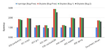
Figure 1: Speedup of Skylake simulation with and without performance bugs, normalized against Ivybridge simulation.

In addition to a bug-free case, we collected performance data for two arbitrarily selected bug-cases for Skylake. Bug 1 is an instruction scheduling bug wherein xor instructions are the only instructions selected to be issued when they are the oldest instruction in the instruction queue. As the figure shows, the overall impact of this bug is very low ($<1\%$ in average across the given workloads). Bug 2 is another instruction scheduling bug which causes sub instructions to be incorrectly marked as synchronizing, thus all younger instructions must wait to be issued after any sub instruction has been issued and all older instructions must issue before any sub instruction, regardless of dependencies and hardware resources. The impact of this bug is larger, at $\sim 7\%$ across the given workloads.

Nevertheless, for both bugs, the impact is less than the difference between Skylake and Ivybridge. Thus, from the designers perspective, working on the newer Skylake design with Ivybridge in hand, if early performance models showed the results shown for Bug 2 (even more so Bug 1) designers might incorrectly assume that the buggy Skylake design did not have performance bugs since it was much better than previous generations. Even as the performance difference between microarchitecture generations decreases, differentiating between performance bugs and expected behavior remains a challenge given the variability between simulated performance and real systems.

Examining the figure, we note that each bug’s impact varies from workload to workload. That said, in the case of Bug 1, no single benchmark shows a performance loss of more than 1%. This makes sense since the bug only impacts the performance of applications which have, relatively rare, xor instructions. From this, one might conclude that Bug 1 is trivial and perhaps needs not be fixed at all. This assumption however, would be wrong, as many workloads do in fact rely heavily upon the xor instruction, enough so that a moderate impact on them translates into significant performance impact overall.

In this work, we explore several approaches to this problem and ultimately develop an automated, two-stage, machine learning-based methodology that will allow designers to automatically detect the existence of performance bugs in microprocessor designs. Even though this work focus is the processor core, we show that the methodology can be used for other system modules, such as the memory. Our approach extracts and exploits knowledge from legacy designs instead of relying on a reference model. Legacy designs have already undergone major debugging, therefore we considered them to be bug-free, or to have only minor performance bugs. The automatic detection takes several minutes of machine learning inference time and several hours of architecture simulation time. The major contributions of this work include the following:

• This is the first study on using machine learning for performance bug detection, to the best of our knowledge. Thus, while we provide a solution to this particular problem, we also hope to draw the attention of the research community to the broader performance validation domain.

• Investigation of different strategies and machine learning techniques to approach the problem. Ultimately, an accurate and straight forward, two phase approach is developed.

• A novel automated method to leverage SimPoints [25] to extract, short, performance-orthogonal, microbenchmark “probes” from long running workloads.

• A set of processor performance bugs which may be configured for an arbitrary level of impact, for use in testing performance debugging techniques is developed.

• Our methodology detects 91.5% of these processor core performance bugs leading to $\geq 1\%$ IPC degradation with 0% false positives. It also achieves 100% accuracy for the evaluated performance bugs in memory systems.

As an early work in this space, we limit our scope somewhat to maintain tractablity. This work is focused mainly on the processor core (the most complex component in the system), however we show that the methodology can be generalized to other units by evaluating its usage on memory systems. Further, here we focus on performance bugs that affect cycle count and consider timing issues to be out of scope.

The goal of this work is to find bugs in new architectures that are incrementally evolved from those used in the training data, it may not work as well when there have been large shifts in microarchitectural details, such as going from in-order to out-of-order. However, major generalized microarchitectural changes are increasingly rare. For example, Intel processors’ last major microarchitecture refactoring occurred $\sim 15$ years ago, from P4 to “Core”. Over this period, there have been several microarchitectures where our approach could provide value. In the event of larger changes, our method can be partially reused by augmenting it with additional features.

II Objective and A Baseline Approach

The objective of this work is the detection of performance bugs in new microprocessor designs. We explicitly look at microarchitectural-level bugs, as opposed to logic or architectural-level bugs. As grounds for the detection, one or multiple legacy microarchitecture designs are available and assumed to be bug-free or have only minor performance bugs remaining. Given the extensive pre-silicon and post-silicon debug, this assumption generally holds on legacy designs. There are no assumptions about how a bug may look like. As it is very difficult to define a theoretical coverage model for performance debug, our methodology is a heuristic approach.

We introduce a naïve baseline approach to solving the bug detection problem. This serves as a prelude for describing our proposed methodology. It also provides a reference for comparison in the experiments.

Performance bug detection bears certain similarity to standard chip functional bug detection. Thus, a testbench strategy similar to functional verification is sensible. That is, a set of microbenchmarks are simulated on the new microarchitecture, and certain performance characteristics are monitored and analyzed. The key difference is that functional verification has correct responses to compare against while bug-free performance for a new microarchitecture is not well defined.

The baseline approach uses supervised machine learning to classify if an microarchitecture has performance bugs or not. The input features for a machine learning model consist of performance counter data, IPC (committed Instructions Per Cycle) and microarchitecture design parameters, such as cache sizes. One classification result on bug existence or not is produced for each application. The overall detection result is obtained by a voting-based ensemble of classification results among multiple applications. Let $\rho$ be the ratio of the number of applications with positive classification (indicating bug) versus the total number of applications. A microarchitecture design is judged to have a bug if $\rho\geq\theta$, where $\theta$ is a threshold determining the tradeoff between true positive and false positive rates. The models are trained by legacy microarchitecture designs and bugs are inserted to obtain labeled data.

The details of this approach, such as applications, machine learning engines, performance counter selection, microarchitecture parameters and bug development, overlap with our proposed method and will be described in later sections.

III Proposed Methodology

III-A Key Idea and Methodology Overview

The proposed methodology is composed of two stages. The first stage consists of a machine learning model trained with performance counter data from bug-free microarchitectures to infer microprocessor performance in terms of IPC. If such model is well-trained and achieves high accuracy, it will capture the correlation between the performance counters and IPC in bug-free microarchitectures. When this model is then applied on designs with bugs, a significant increase in inference errors is expected, as the bugs ruin the correlation between the counters and IPC. The second stage determines bug existence due to the IPC inference errors in the first stage. An overview of the two-stage methodology is depicted in Figure 2. Although in this work we evaluate the methodology using only microarchitecture simulations, its key idea is generic and can be extended for FPGA prototyping or post-silicon testing. The applicability in both pre- and post-silicon validations is a strong point of our methodology, especially as some bugs might be triggered by traces that are too long to be simulated.

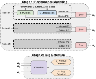
Figure 2: Overview of the proposed methodology.

In this methodology, a microbenchmark and a set of selected performance counters form a performance probe. Probe design is introduced in Section III-B. The machine learning model is applied on individual probes for IPC inference, which is described in Section III-C. The classification in stage two is based on the errors from multiple probes, and elaborated in Section III-D.

III-B Performance Probe Design

III-B1 SimPoint-Based Microbenchmark Extraction

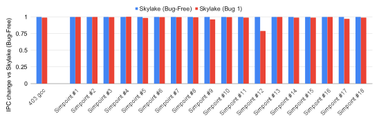
Figure 3: IPC by SimPoints in 403.gcc for Skylake architecture.

Finding the right applications to use in “probing” the microarchitecture for performance bugs is critical to the efficiency and efficacy of the proposed methodology. One possible approach could be to meticulously hand generate an exhaustive set of microbenchmarks to test all the interacting components of the microarchitecture under all possible instruction orderings, branch paths, dependencies, etc. This approach is similar to that taken in some prior works [16, 38, 17]. While this approach would likely be possible, automating the process as much as possible is highly desirable, given the overheads already required for verification and validation. Thus, another key goal of our work is to automatically find and select short, orthogonal and relevant performance microbenchmarks to use in the microarchitecture probing.

Typically in computer architecture research, large, orthogonal suites of workloads, such as the SPEC CPU suites [2, 3], are used for performance benchmarking. The applications in these suites, however, typically are too large to simulate to completion. Thus, development of statistically accurate means to shorten benchmark runtimes has received significant attention [12, 56, 48]. One notable work was SimPoints [48, 24, 25], wherein the authors propose to identify short, performance-orthogonal segments of long running applications. These segments are simulated separately and the whole application performance is estimated as a weighted average of the performance of those points. In this work, we propose a novel use of the SimPoints methodology. Instead of using them as intended, for performance estimation of large applications, we propose to use them to automatically identify and extract short, orthogonal, performance-relevant microbenchmarks from long running applications. Here we are leveraging SimPoints’ identification of orthogonal basic-block vectors in the given program to be the source of our orthogonal microbenchmarks.

As an example how this provides greater visibility into performance bugs, consider Figure 3. In the figure, we compare the performance per SimPoint of bug-free and Bug 1 versions of Skylake (described in Section I) for the benchmark 403.gcc. We see that, although the overall difference in the whole application is less than 1%, when we split the performance by SimPoint, SimPoint #12 has a degradation of over 20%, making Bug 1’s behavior much easier to identify as incorrect.

The reason why SimPoint #12 shows this behavior is because it has more than twice the number of xor operations than the others, accounting for 2.3% of all instructions executed here. We argue that, even though the overall impact on the performance in 403.gcc is very low, this particular SimPoint represents well a class of applications with similar behavior that would not be represented by looking at any single benchmark in the SPEC CPU suite. Thus, by utilizing SimPoints individually more performance bug coverage can be gained than by looking at full application performance.

III-B2 Performance Counter Selection

Performance counter data from microbenchmark simulation constitute the main features for our machine learning models to infer overall performance. Hence, they are essential components for the performance probes. We note that, as part of the design cycle, performance counters often undergo explicit validation. The assumption of their sanity is central for performance debug in general, not only this methodology.

Microprocessors typically contain hundreds to thousands of performance counters. Using all of them as features would unnecessarily extend training and inference time for machine learning models, and even degrade them as some useless counters may blur the picture. Hence, we select a small subset of them for each microbenchmark that is sufficient for effective machine learning inference on that workload. We note that the abundance of counters along with our selection method makes our methodology resilient to small changes in the counters available across different generations of architecture designs.

The selection is carried out in two steps.

• Step 1: The Pearson correlation coefficient is evaluated for each counter with respect to IPC. Only those counters with high correlations with IPC (magnitude greater than 0.7) are retained and the others are pruned out.

• Step 2: Among the remaining counters, the correlation between every pair of them is evaluated. If two counters have a Pearson correlation coefficient whose magnitude is greater than 0.95, we consider them redundant and one of them is pruned out.

Counter selection is conducted independently for each probe and thus different probes may use different counters. Examples of the most commonly selected counters are: the number of fetched instructions, percentage of branch instructions, number of writes to registers, percentage of correctly predicted indirect branches, number of cycles on which the maximum possible number of instructions were committed, among others.

III-C Stage 1: Performance Modelling

Stage 1 of our methodology models overall processor performance (IPC), via machine learning. Among innumerable possible ways to perform such task, we elaborately develop one with the following key ingredients:

1. The training data are taken from (presumably) bug-free designs. Otherwise, the inference errors between bug-free designs and bug cases cannot be differentiated.

2. One model is trained for each probe. As workload characteristics of different probes can be drastically different, it is very difficult (also unnecessary), for a single model to capture them all. A separated model for each probe is necessary to achieve high accuracy for bug-free designs. This is a key difference from previous methods of performance counter-based predictions where a single model is derived to work across many different workload [32, 13, 7, 57]. By tuning our model to the particular counters relevant to a particular probe workload, much higher accuracy can be achieved.

3. Models are trained with a variety of microarchitectures. This ensures that inference error differences are due to existence of bugs instead of microarchitecture difference. In practice, the training is performed on legacy designs and the model inference would be on a new microarchitecture.

4. The input features are taken as a time series. The simulation (or running system) proceeds over a series of time steps $t_{1},t_{2},...$. Let the current time step be $t_{i}$, then the model takes feature data of $t_{i-w+1},t_{i-w+2},...,t_{i-w+w}$ as input to estimate IPC at $t_{i}$, where $w$ is the window size. Usually, a time step consists of multiple clock cycles, e.g., a half million cycles. If one intends to take the aggregated data of an entire SimPoint as input, that is a special case of our framework, where the step size is the entire SimPoint and the window size is 1.

Besides the selected counters discussed in Section III-B2, some microarchitecture design parameters are used as features to our machine learning model. They include clock cycle, pipeline width, re-order buffer size and some cache characteristics such as latency, size and associativity. Please note that the parameter features are constant in the time series input for a specific microarchitecture.

The following machine learning engines are investigated for per-probe IPC inference in this work

Linear Regression (Lasso) This is a simple linear regression algorithm [49], of the form $y=\mathbf{x}^{T}\mathbf{w}$, where $\mathbf{w}$ is the vector of parameters. It uses L1 regularization on the values of $\mathbf{w}$. The main advantage of this model is its simplicity.

Multi-Layer Perceptron (MLP) This classical neural network consists of multiple layers of perceptrons. Each perceptron takes a linear combination of signals of the previous layer and generates an output via a non-linear activation function [28].

Convolutional Neural Network (CNN) This neural network architecture contains convolution operations and the parameters of its convolution kernel are trained with data [36]. In this work, the features are taken as 1D vector as described by Eren et al. [20] and Lee et al. [37], as opposed to 2D images.

Long Short-Term Memory Network (LSTM) This is a form of recurrent neural network, where the output depends not only on the input but also internal states [27]. The states are useful in capturing history effect and make LSTM effective for handling time series signals.

Gradient Boosted Trees (GBT) This is a decision tree-based approach, where a branch node in the tree partitions the feature space and the leaf nodes tell the inference results. The overall result is an ensemble of results from multiple trees [21]. In this work, we adopt XGBoost [10], which is the latest generation of GBT approach.

Consider a set of probes $P=\{p_{1},p_{2},...\}$. A trained model is applied to infer IPC $\hat{y}_{i,j}$ for time step $t_{j}$ of probe $p_{i}$ for a particular design, while the corresponding IPC by simulation is $y_{i,j}$. For each probe $p_{i}\in P$, the inference error is

$$\Delta_{i}=\frac{1}{2}\sum_{j=2}^{T_{i}}\left(|y_{i,j}-\hat{y}_{i,j}|+|y_{i,j-1}-\hat{y}_{i,j-1}|\right)$$ (1)

where $T_{i}$ is the number of time steps in $p_{i}$. This error can be interpreted as the area of difference between the inferred IPC over time and the actual (simulated) IPC. It is also approximately equal to the total absolute error. The set of errors $\{\Delta_{1},\Delta_{2},...,\Delta_{|P|}\}$ are fed to stage 2 of our methodology. Empirically, this error metric outperforms others, such as Mean Squared Error (MSE), in the bug classification of stage 2. An advantage of error metric (1) is that a large error in a single (or few) time step(s) is not averaged out, as it is with MSE.

Our machine learning models are not intended to be golden performance models. Instead, each model captures the complex relationship between counters and performance for the workload in exactly one probe. Their comparison against the simulated performance for that particular probe is not to determine if performance is satisfactory, rather it is to attempt to detect if the model accuracy is ruined, as this might signal the relations between counters and performance are broken, therefore a performance bug is likely. The usage of machine learning is essential for bug detection as it overcomes the difficulty to obtain a single, accurate, universal bug-free performance model.

III-D Stage 2: Bug Detection

Given a vector $[\Delta_{1},\Delta_{2},\cdots,\Delta_{|P|}]$ of IPC inference errors from stage 1, the purpose of stage 2 is to identify if a bug exists in the corresponding microarchitecture. In general, a small $\Delta_{i}$ error indicates that the machine learning model in stage 1, which is trained with bug-free designs, matches well the design under test and hence likely no bugs (with respect to that probe). On the other hand, large $\Delta_{i}$ error indicates a large likelihood of bugs. Bugs can reside at different locations and manifest in a variety of ways. Therefore, multiple orthogonal probes are necessary to improve the breadth and robustness of the detection, as highlighted in the case of Bug 1 in Figure 3.

Although we considered using a machine learning classifier for stage 2, we found the available training data for this stage to be much more scarce than that of stage 1. For stage 1, every time step of the collected data represents a data sample, making thousands of samples available. In contrast, only one data sample per microarchitecture is available for stage 2, making only a few dozens of samples available. To overcome the lack of data available for training we developed a custom rule-based classifier.

Suppose there are $m$ positive samples (with bugs) and $n$ negative samples (bug-free). For each probe $p_{i}\in P$, we compute the mean $\mu_{i}^{+}$ and standard deviation $\sigma_{i}^{+}$ of the IPC inference errors among the $m$ positive samples. Similarly, we can obtain $\mu_{i}^{-}$ and $\sigma_{i}^{-}$ among the $n$ negative samples for each $p_{i}\in P$. These statistics form a reference to evaluate the IPC inference errors for a new architecture.

For the error $\Delta^{\prime}_{i}$ of applying probe $p_{i}$ on the new architecture, we evaluate the following ratios based on the statistics of the labeled data.

$$\gamma_{i}^{+}=\frac{\Delta^{\prime}_{i}}{\mu_{i}^{+}+\alpha\sigma_{i}^{+}}~{},~{}~{}\gamma_{i}^{-}=\frac{\Delta^{\prime}_{i}}{\mu_{i}^{-}+\alpha\sigma_{i}^{-}}$$ (2)

where $\alpha$ is a parameter trained with the labeled data. In general, a large value of $\Delta^{\prime}_{i}$ signals a high probability of bugs in the new microarchitecture. Ratios $\gamma_{i}^{+}$ and $\gamma_{i}^{-}$ are relative to the labeled data, and make the errors from different probes comparable.

Given vectors $[\gamma_{1}^{+},\gamma_{2}^{+},...,\gamma_{|P|}^{+}]$ and $[\gamma_{1}^{-},\gamma_{2}^{-},...,\gamma_{|P|}^{-}]$, our classifier is a rule-based recipe as follows.

1. If $\max(\gamma_{1}^{+},\gamma_{2}^{+},...,\gamma_{|P|}^{+})>\eta$, where $\eta$ is a parameter, this architecture is classified to have bugs. This is for the case where a large error appears in at least one probe regardless of errors from the other probes.

2. If $(\gamma_{1}^{-}+\gamma_{2}^{-}+...+\gamma_{|P|}^{-})/|P|>\lambda$, where $\lambda<\eta$ is a parameter, this architecture is classified to have bugs. This is for the case where small errors appear on many probes.

3. For other cases, the architecture is classified as bug-free.

While the values of $\eta$ and $\lambda$ are empirically chosen as 15 and 5, respectively, the value of $\alpha$ is trained according to true positive rate and false positive rate on the labeled data. In the training, a set of uniformly spaced values in a range are tested for $\alpha$, and the one with the maximum true positive rate and false positive rate no greater than 0.25 is chosen.

IV Experimental Setup

In this section we elaborate on the details of the implementation of our methodology. Sections IV-A to IV-C cover the experimental setup for processor core performance bugs, since this is the main focus of our work, we provide detailed explanations. Section IV-D lists the changes implemented for the memory system performance bug detection.

IV-A Probe Setup

The performance probes are extracted from 10 applications from the SPEC CPU2006 benchmark [2] using the SimPoints methodology [25], as described in Section III-B1. We chose to use SPEC CPU2006 instead of the more recent SPEC CPU2017 suite because their relatively smaller memory footprints, generally reduced running times and computational resources needed to detect performance bugs, though there is no reason our techniques would not work with SPEC CPU2017 applications. Unlike developing performance improvement techniques, where the benchmarks serve as testcases and should be exhaustively used, the selected applications here are part of our methodology implementation. In fact, the selection affects the tradeoff between the efficacy of detection and runtime overhead of the methodology, as we will show.

There are 190 SimPoints in total for the ten SPEC CPU2006 applications we use here and each SimPoint contains around 10M instructions. The applications we selected in particular were an arbitrary set of the first 10 we were able to compile and run in gem5 across all microarchitectures. Adding more benchmarks would only improve the results we achieve. A list of the applications is provided in Table I.

For each probe, between 4 and 64 performance counters are selected using the methodology detailed in Section III-B2. The time step size is 500k clock cycles. That is, for each counter, a value is recorded every 500k clock cycles. The values of all time steps form the time series as input feature to the machine learning models. As the time step size is sufficiently large, the default window size (see Section III-C) is one time step.

TABLE I: Selected SPEC CPU2006 benchmarks.

Benchmark	Operand Type	Application	SimPoints
400.perlbench	Integer	PERL Programming Language	14
401.bzip2	Integer	Compression	23
403.gcc	Integer	C Compiler	18
426.mcf	Integer	Combinatorial Optimization	15
433.milc	Floating Point	Quantum Chromodynamics	20
436.cactusADM	Floating Point	General Relativity	16
444.namd	Floating Point	Molecular Dynamics	26
450.soplex	Floating Point	Linear Programming	21
458.sjeng	Integer	AI: Chess	19
462.libquantum	Integer	Quantum Computing	18

IV-B Simulated Architectures

All experiments are performed via gem5 [6] simulations in System Emulation mode. Note, the key ideas of our methodology can be implemented in other simulators and post-silicon debug. Here we are focused on core performance bugs, thus we use the Out-Of-Order core (O3CPU) model with the x86 ISA. Gem5 is configured to model different architectures by varying several configuration variables such as clock period, re-order buffer size, cache size, associativity, latency, and number of levels, as well as functional unit count, latency, and port organization. Besides these common knobs, other microarchitectural differences between designs are not considered. The configurations model eight different existing microarchitectures: Intel Broadwell, Cedarview, Ivybridge, Skylake and Silvermont, AMD Jaguar, K8, and K10, as well as 12 artificial microarchitectures with realistic settings. With these, we achieve a wide variety of architectures, from low-power systems such as Silvermont to high-performance server systems such as Skylake. Detailed information of the specifications used for each architecture can be found in Table II. Table III describes the port organization for each of the architectures. These microarchitectures serve as training data for machine learning models and unseen data for testing the models. They are partitioned into four disjoint sets as follows.

• Set I: Contains two real and seven artificial microarchitectures. They are used to train our IPC models.

• Set II: Three microarchitectures in this set, a real one and two artificial ones, play the role of validation in training the IPC models. That is, a training process terminates after 100 epochs of training without improvement on this set. In addition, this set serves as labeled data for training the classifier in stage 2.

• Set III: Four microarchitectures, one real and three artificial, are used as additional training data for the stage 2 classifier. As such, the training data for stage 2 is composed by set II and III. This is to decouple the training data between stage 1 and stage 2.

• Set IV: Four microarchitectures in this set are for the testing of the stage 2 classifier. As stage 2 is the eventual bug detection, all of the four microarchitectures here are real ones so as to ensure the overall testing is realistic.

TABLE II: Architectural knobs for implemented architectures.

Set	Architecture	Clock Cycle	CPU Width	ROB Size	L1 Cache (Size / Assoc. / Latency)	L2 Cache (Size / Assoc. / Latency)	L3 Cache (Size / Assoc. / Latency)	Func. Unit Latency (FP / Multiplier / Divider)
I	Broadwell	4.0GHz	4	192	32kB / 8-way / 4 cycles	256kB / 8-way / 12 cycles	64MB / 16-way / 59 cycles	5 cycles / 3 cycles / 20 cycles
I	Cedarview	1.8GHz	2	32	32kB / 8-way / 3 cycles	512kB / 8-way / 15 cycles	No L3	5 cycles/ 4 cycles / 30 cycles
I	Jaguar	1.8GHz	2	56	32kB / 8-way / 3 cycles	2MB / 16-way / 26 cycles	No L3	4 cycles / 3 cycles / 20 cycles
I	Artificial 2	4.0GHz	8	168	32kB / 2-way / 5 cycles	256kB / 8-way / 16 cycles	No L3	4 cycles / 4 cycles / 20 cycles
I	Artificial 3	3.0GHz	8	32	32kB / 2-way / 3 cycles	512kB / 16-way / 24 cycles	8MB / 32-way / 52 cycles	4 cycles / 4 cycles / 20 cycles
I	Artificial 4	4.0GHz	2	192	64kB / 8-way / 3 cycles	1MB / 8-way / 20 cycles	32MB / 16-way / 28 cycles	5 cycles / 3 cycles / 20 cycles
I	Artificial 6	3.5GHz	4	192	64kB / 8-way / 4 cycles	1MB / 8-way / 16 cycles	8MB / 32-way / 36 cycles	4 cycles / 4 cycles / 20 cycles
I	Artificial 7	3.0GHz	4	32	16kB / 8-way / 3 cycles	512kB / 16-way / 12 cycles	32MB / 32-way / 28 cycles	2 cycles / 7 cycles / 69 cycles
I	Artificial 10	1.5GHz	8	32	32kB / 2-way / 2 cycles	256kB / 16-way / 24 cycles	64MB / 32-way / 36 cycles	5 cycles/ 4 cycles / 30 cycles
I	Artificial 11	3.5GHz	4	32	64kB / 4-way / 5 cycles	256kB / 4-way / 24 cycles	No L3	5 cycles/ 4 cycles / 30 cycles
II	Ivybridge	3.4GHz	4	168	32kB / 8-way / 4 cycles	256kB / 8-way / 11 cycles	16MB / 16-way / 28 cycles	5 cycles / 3 cycles / 20 cycles
II	Artificial 0	2.5GHz	4	192	64kB / 2-way / 4 cycles	512kB / 4-way / 12 cycles	No L3	5 cycles / 3 cycles / 20 cycles
II	Artificial 9	3.5GHz	8	192	16kB / 4-way / 5 cycles	1MB / 4-way / 20 cycles	64MB / 16-way / 44 cycles	4 cycles / 3 cycles / 11 cycles
III	Artificial 1	1.5GHz	4	192	64kB / 8-way / 5 cycles	2MB / 8-way / 16 cycles	No L3	4 cycles / 3 cycles / 11 cycles
III	Artificial 5	3.5GHz	2	32	32kB / 4-way / 5 cycles	256kB / 4-way / 16 cycles	8MB / 32-way / 44 cycles	4 cycles / 3 cycles / 11 cycles
III	Artificial 8	3.0GHz	2	192	32kB / 2-way / 2 cycles	1MB / 16-way / 16 cycles	32MB / 32-way / 52 cycles	4 cycles / 3 cycles / 11 cycles
IV	K8	2.0GHz	3	24	64kB / 2-way / 4 cycles	512kB / 16-way / 12 cycles	No L3	4 cycles / 3 cycles / 11 cycles
IV	K10	2.8GHz	3	24	64kB / 2-way / 4 cycles	512kB / 16-way / 12 cycles	6MB / 16-way / 40 cycles	4 cycles / 3 cycles / 11 cycles
IV	Silvermont	2.2GHz	2	32	32kB / 8-way / 3 cycles	1MB / 16-way / 14 cycles	No L3	2 cycles / 7 cycles / 69 cycles
IV	Skylake	4.0GHz	4	256	32kB / 8-way / 4 cycles	256kB / 4-way / 12 cycles	8MB / 16-way / 34 cycles	4 cycles / 4 cycles / 20 cycles

TABLE III: Port organization of implemented architectures.

Set	Architecture	Port 0	Port 1	Port 2	Port 3	Port 4	Port 5	Port 6
I	Broadwell	1 ALU, 1 FP Mult 1 FP unit, 1 Int Vector 1 Int Mult, 1 Divider 1 Branch Unit	1 ALU, 1 Vector Unit 1 FP Mult, 1 Int Mult	1 Load Unit	1 Load Unit	1 Store Unit	1 ALU, 1 Vector Unit	1 ALU, 1 Branch Unit
I	Cedarview	1 ALU, 1 Load Unit 1 Store Unit, 1 Vector Unit 1 Int Mult, 1 Divider	1 ALU, 1 Vector Unit 1 FP Unit, 1 Branch Unit	1 Load Unit	1 Store Unit	-	-	-
I	Jaguar	1 ALU, 1 Vector Unit	1 ALU, 1 Vector Unit	1 FP Unit, 1 Int Mult	1 FP Mult, 1 Divider	1 Load Unit	1 Store Unit	-
I	Artificial 2	1 ALU, 1 Vector Unit 1 FP Unit, 1 Int Mult 1 Divider, 1 Branch Unit	1 ALU, 1 Vector Unit 1 FP Mult, 1 FP Unit 1 Int Mult	1 Load Unit	1 Load Unit	1 Store Unit	1 ALU, 1 Vector Unit	1 ALU, 1 Branch Unit
I	Artificial 3	1 ALU, 1 Vector Unit 1 FP Unit, 1 Int Mult 1 Divider, 1 Branch Unit	1 ALU, 1 Vector Unit 1 FP Mult, 1 FP Unit 1 Int Mult	1 Load Unit	1 Load Unit	1 Store Unit	1 ALU, 1 Vector Unit	1 ALU, 1 Branch Unit
I	Artificial 4	1 ALU, 1 FP Mult 1 FP unit, 1 Int Vector 1 Int Mult, 1 Divider 1 Branch Unit	1 ALU, 1 Vector Unit 1 FP Mult, 1 Int Mult	1 Load Unit	1 Load Unit	1 Store Unit	1 ALU, 1 Vector Unit	1 ALU, 1 Branch Unit
I	Artificial 6	1 ALU, 1 Vector Unit 1 FP Unit, 1 Int Mult 1 Divider, 1 Branch Unit	1 ALU, 1 Vector Unit 1 FP Mult, 1 FP Unit 1 Int Mult	1 Load Unit	1 Load Unit	1 Store Unit	1 ALU, 1 Vector Unit	1 ALU, 1 Branch Unit
I	Artificial 7	1 Load Unit, 1 Store Unit	1 ALU, 1 Integer Mult	1 ALU, 1 Branch Unit	1 FP Mult, 1 Divider	1 FP Unit	-	-
I	Artificial 10	1 ALU, 1 Load Unit 1 Store Unit, 1 Vector Unit 1 Int Mult, 1 Divider	1 ALU, 1 Vector Unit 1 FP Unit, 1 Branch Unit	1 Load Unit	1 Store Unit	-	-	-
I	Artificial 11	1 ALU, 1 Load Unit 1 Store Unit, 1 Vector Unit 1 Int Mult, 1 Divider	1 ALU, 1 Vector Unit 1 FP Unit, 1 Branch Unit	1 Load Unit	1 Store Unit	-	-	-
II	Ivybridge	1 ALU, 1 Vector Unit 1 FP Mult, 1 Divider	1 ALU, 1 Vector Unit 1 Int Mult, 1 FP Unit	1 Load Unit	1 Load Unit	1 Store Unit	1 ALU, 1 Vector Unit 1 Branch Unit, 1 FP Unit	-
II	Artificial 0	1 ALU, 1 FP Mult 1 FP unit, 1 Int Vector 1 Int Mult, 1 Divider 1 Branch Unit	1 ALU, 1 Vector Unit 1 FP Mult, 1 Int Mult	1 Load Unit	1 Load Unit	1 Store Unit	1 ALU, 1 Vector Unit	1 ALU, 1 Branch Unit
II	Artificial 9	1 ALU, 1 Vector Unit 1 Int Mult	1 ALU, 1 Vector Unit	1 ALU, 1 Vector Unit	1 Load Unit	1 Store Unit	1 FP Unit	1 FP Unit
III	Artificial 1	1 ALU, 1 Vector Unit 1 Int Mult	1 ALU, 1 Vector Unit	1 ALU, 1 Vector Unit	1 Load Unit	1 Store Unit	1 FP Unit	1 FP Unit
III	Artificial 5	1 ALU, 1 Vector Unit 1 Int Mult	1 ALU, 1 Vector Unit	1 ALU, 1 Vector Unit	1 Load Unit	1 Store Unit	1 FP Unit	1 FP Unit
III	Artificial 8	1 ALU, 1 Vector Unit 1 Int Mult	1 ALU, 1 Vector Unit	1 ALU, 1 Vector Unit	1 Load Unit	1 Store Unit	1 FP Unit	1 FP Unit
IV	K8	1 ALU, 1 Vector Unit 1 Int Mult	1 ALU, 1 Vector Unit	1 ALU, 1 Vector Unit	1 Load Unit	1 Store Unit	1 FP Unit	1 FP Unit
IV	K10	1 ALU, 1 Vector Unit 1 Int Mult	1 ALU, 1 Vector Unit	1 ALU, 1 Vector Unit	1 Load Unit	1 Store Unit	1 FP Unit	1 FP Unit
IV	Silvermont	1 Load Unit, 1 Store Unit	1 ALU, 1 Integer Mult	1 ALU, 1 Branch Unit	1 FP Mult, 1 Divider	1 FP Unit	-	-
IV	Skylake	1 ALU, 1 Vector Unit 1 FP Unit, 1 Int Mult 1 Divider, 1 Branch Unit	1 ALU, 1 Vector Unit 1 FP Mult, 1 FP Unit 1 Int Mult	1 Load Unit	1 Load Unit	1 Store Unit	1 ALU, 1 Vector Unit	1 ALU, 1 Branch Unit

IV-C Bug Development

To the best of our knowledge, gem5 is a performance bug-free simulator. To achieve wide bug representation we reviewed errata of commercial processors, consulted with industry experts and tried to cover as many units as possible. Ultimately, 14 basic types of bugs are developed and are summarized as follows.

1. Serialize X: Every instruction with opcode of X is marked as a serialized instruction. This causes all future instructions (according to program order) to be stalled until the instruction with the bug has been issued.

2. Issue X only if oldest: Instructions whose opcode is X will only be retired from the instruction queue when it has become the oldest instruction there. This bug is similar to “POPCNT Instruction may take longer to execute than expected” found on Intel Xeon Processors [31].

3. If X is oldest, issue only X: When an instruction whose opcode is X becomes the oldest in the instruction queue, only that instruction will be issued, even though other instructions might also be ready to be issued and the computation resources allow it.

4. If X depends on another instruction Y, delay T cycles.

5. If less than N slots available in instruction queue, delay T cycles.

6. If less than N slots available in re-order buffer, delay T cycles.

7. If mispredicted branch, delay T cycles.

8. If N stores to cache line, delay T cycles: After N stores have been executed to the same cache line, upcoming stores to the same line will be delayed by T cycles. This is a variation of “Store gathering/merging performance issue” found on NXP MPC7448 RISC processor [45].

9. After N stores to the same register, delay T cycles. This bug is inspired by “GPMC may Stall After 256 Write Accesses in NAND_DATA, NAND_COMMAND, or NAND_ADDRESS Registers” found on TI AM3517, AM3505 ARM processor [54], we generalized it for any physical register, and in our case, the instruction is only stalled for a few cycles, as opposed to the actual bug, where the processor hanged. Another variation of this bug is implemented where the delay is applied once every N stores, instead of every store after the N-th.

10. L2 cache latency is increased by T cycles. This bug is inspired by the “L2 latency performance issue” on the NXP MPC7448 RISC processor [45].

11. Available registers reduced by N.

12. If branch longer than N bytes, delay T cycles.

13. If X uses register R, delay T cycles. This bug is a variation of the “POPA/POPAD Instruction Malfunction” found on Intel 386 DX [30].

14. Branch predictor’s table index function issue, reducing effective table size by N entries.

For each of these bug types, multiple variants are implemented by changing X, Y, N, R and T respectively. The bugs are grouped into four categories according to their impact on IPC: High means an average IPC degradation (across the used SPEC CPU2006 applications) of 10% or greater. A Medium impact means the average IPC is degraded between 5% and 10%. A Low impact is between 1% and 5% and a Very-Low impact is less than 1%. Figure 4 shows the distribution of the severity of average IPC impact for the implemented bugs.

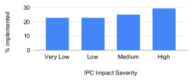
Figure 4: Distribution of bug severity.

IV-D Bug Detection in Memory Systems

We also examine the performance of the proposed methodology on areas outside of the processor core, specifically on the processor cache memory system. Overall the methodology remains unchanged, but there are some minor differences vs. the evaluation of our technique on processor cores. Here we use the ChampSim [1] simulator instead of gem5 [6], because it provides a more detailed memory system simulation with relatively short simulation time. ChampSim was developed for rapid evaluation of microarchitectural techniques in the processor cache hierarchy.

The probes we use for this evaluation correspond to 22 SimPoints from seven applications on the SPEC CPU2006 [2] benchmark suite. The emulated architectures are Intel’s Broadwell, Haswell, Skylake, Sandybridge, Ivybridge, Nehalem and AMD’s K10 and Ryzen7, as well as four artificial architectures. The developed bugs are summarized as follows.

1. When a cache block is accessed, the age counter for the replacement policy is not updated.

2. During a cache eviction, the policy evicts the most recently used block, instead of the least recently used.

3. After N load misses on L1D cache, the read operation is delayed by T clock cycles. Another variant of this bug was implemented for L2 cache.

4. Signature Path Prefetcher (SPP) [34] signatures are reset, making the prefetcher use the wrong address.

5. On lookahead prefetching, the path with the least confidence is selected.

6. Some prefetches are incorrectly marked as executed. This bug was found in the SPP [34] prefetching method.

Since IPC might be affected by many other factors outside the memory system, we evaluate our methodology by using Average Memory Access Time (AMAT) as the target metric for the performance models. Given the differences between simulators, architectures and bugs, the rules for stage 2 were slightly modified for this evaluation, however, the overall methodology remains unchanged.

V Evaluation

Since the main focus of our work is on the processor core, sections V-A to V-H examine performance bugs in that unit. Section V-I expands examination to memory system bugs.

V-A Machine Learning-Based IPC Modeling

In this section, we show the results for the first stage of our methodology, IPC modelling. We evaluated the performance of several machine learning methods, as discussed in Section III-C, and different variations for each of them. The MLP, CNN and LSTM networks are implemented using Keras library [11]. In training all these models, Mean Squared Error (MSE) is used as the loss function and Adam [35] is employed as the optimizer. A gradient clipping of $0.01$ is enforced to avoid the gradient explosion issue, commonly seen in training recurrent networks. The gradient boosted trees are implemented via the XGBoost library [10]. Lasso is implemented using Scikit-Learn [47].

The total (all probes) training and inference runtime, as well as inference error (Eq. 1) for each IPC modelling technique are shown in Table IV. The name of each neural network-based method (LSTM, CNN and MLP), is prefixed with a number indicating the number of hidden layers, and postfixed with the number of neurons in each hidden layer. The postfix number for a GBT method is the number of trees. Runtime results are measured on an Intel Xeon E5-2697A V4 processor with frequency of 2.6GHz and 512GB memory. The total simulation time for detecting bugs in one new microarchitecture takes about 6 hours if the simulations are not executed in parallel.

TABLE IV: IPC modelling runtime and error statistics.

	Runtime		Inference Error (Equation (1))
ML Model	Training	Inference	Average	Std. Dev.	Median	90th Perc.
Lasso	0h 8m	3m 06s	10.2749	2.1598	10.3995	13.1740
1-LSTM-150	3h 22m	16m 21s	$2.87\times 10^{7}$	$2.89\times 10^{8}$	2.8082	5.4062
1-LSTM-250	4h 17m	17m 28s	$4.94\times 10^{23}$	$6.71\times 10^{24}$	2.8364	5.4582
1-LSTM-500	3h 39m	24m 18s	$1.2\times 10^{6}$	$1.63\times 10^{7}$	2.9193	4.7848
4-LSTM-150	4h 39m	54m 33s	$5.81\times 10^{7}$	$5.87\times 10^{8}$	5.5581	13.2453
4-LSTM-500	2h 54m	71m 20s	$1.09\times 10^{3}$	$1.35\times 10^{4}$	4.3551	11.7138
1-CNN-150	0h 19m	08m 16s	5.3959	5.3458	3.4171	17.1287
4-CNN-150	0h 33m	15m 53s	5.7568	5.4779	3.5433	16.2600
1-MLP-500	1h 38m	08m 39s	2.2506	1.5636	1.8200	4.2648
1-MLP-2500	1h 51m	07m 01s	2.1298	1.6228	1.6589	4.4684
4-MLP-500	3h 19m	10m 05s	9.8390	66.6996	4.1207	6.6891
GBT-150	0h 30m	5m 01s	3.7928	2.1445	3.3095	6.3616
GBT-250	0h 38m	4m 34s	3.6181	2.0607	3.1275	6.1395

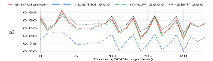
(a) SimPoint #12 of gcc

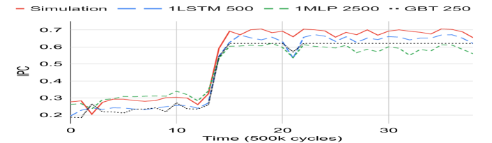
(b) SimPoint #16 of bzip2

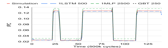
(c) SimPoint #1 of cactusADM

Figure 5: Examples of ML-based IPC inference and simulated IPC on bug-free microarchitectures.

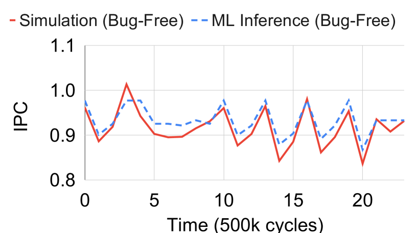
(a) Bug-Free SimPoint #12 in gcc

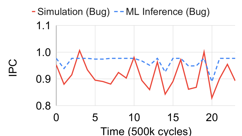
(b) Bug SimPoint #12 in gcc

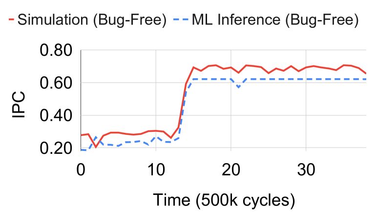
(c) Bug-Free SimPoint #16 in bzip2

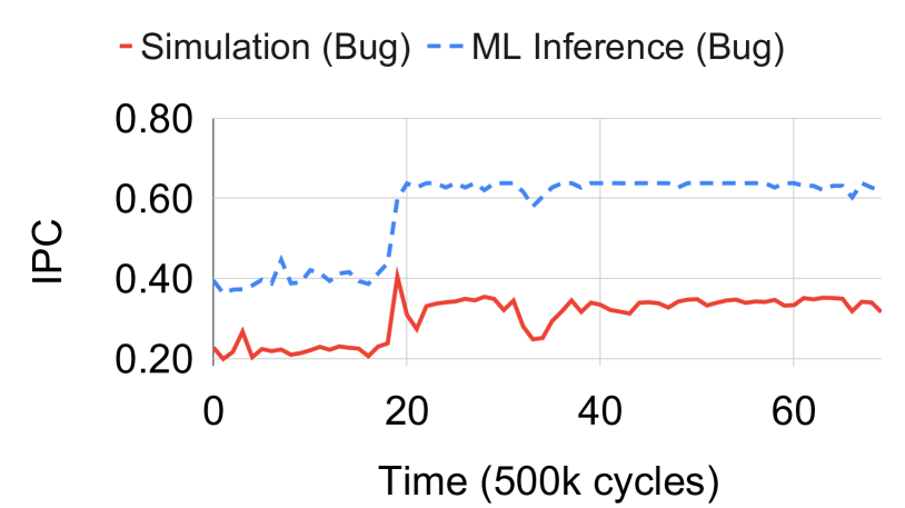
(d) Bug SimPoint #16 in bzip2

Figure 6: IPC estimations by GBT-250: comparisons between microarchitectures with and without bugs.

The right four columns of Table IV summarize the inference errors defined in Equation (1). Please note IPC inference is a regression task, not classification. Thus, classification metrics, such as true positive and false positive rates, do not apply. The results are averaged across all probes for bug-free designs of microarchitectures in Set IV. Median errors of different ML engines are close to each other. LSTM has huge variances and average errors due to a few non-convergent outliers. Although input features are a time series, where LSTM should excel, the actual LSTM errors here are no better than non-recurrent networks and sometimes much worse. There are two reasons for this. First, the time step size we chose is large enough such that the history effect has already been well counted in one time step and thus the recurrence in LSTM becomes unnecessary. Second, LSTM is well-known to be difficult to train and the difficulty is confirmed by those outlier cases. In stage 2 of our methodology, LSTM results with huge errors are not used.

Figure 5 displays the IPC time series for three SimPoints (chosen to represent varied behavior), on the Skylake microarchitecture, where the red solid lines indicate the measured (simulated) IPCs, while the dotted/dashed lines are IPC inferences of the different ML engines. In general, the ML models trace IPCs very well. LSTM has relatively large errors in Figure 5(a), yet it still shows strong correlation with the simulated IPCs. In all three cases the results confirm the effectiveness of the machine learning models across various scenarios.

Although IPC inference accuracy for bug-free designs is important, the inference error difference between cases with and without bugs matters even more. Such difference is illustrated for two SimPoints in Figure 6. In Figure 6(a), where the microarchitecture is bug-free, GBT-250 estimates IPCs very accurately. When there is a bug, however, as shown in Figure 6(b), the inference errors drastically increase. The same discrepancy is also exhibited between another bug-free design, Figure 6(c), and buggy design, Figure 6(d). Both the examples demonstrate that a significant loss of accuracy implies bug existence.

V-B Bug Detection

In this section, we show the evaluation results for our stage 2 classification given the IPC inference errors from stage 1. The evaluation includes comparisons with the naïve single-stage baseline approach described in Section II. The probe designs of the baseline are the same as our proposed methodology. Here we only use the GBT-250 engine which has the best single-stage results. Its model features include simulated IPCs in addition to data from the selected counters and microarchitectural design parameters. However, it uses a single value for each feature aggregated from an entire SimPoint instead of the time series.

The bug detection efficacy is evaluated by the metrics below.

$$\textrm{FPR}=\frac{\textrm{FP}}{\textrm{N}},~{}~{}\textrm{Precision}=\frac{\textrm{TP}}{\textrm{TP}+\textrm{FP}},~{}~{}\textrm{TPR}=\frac{\textrm{TP}}{\textrm{P}}$$ (3)

where N and P are the number of real negative (no bug) and positive (bug) cases, respectively. FP (False Positive) indicates the number of cases that are incorrectly classified as having bugs. TP (True Positive) is the number of cases that are correctly classified as having bugs. Additionally, ROC (Receiver Operating Characteristic) AUC (Area Under Curve) is evaluated. ROC shows the trade-off between TPR and FPR. ROC AUC value varies between 0 and 1. A random guess would result in ROC AUC of 0.5 and a perfect classifier can achieve 1. Accuracy, another common metric, is not employed here as the number of negative cases is too small, i.e., the testcases are imbalanced.

TABLE V: Bug detection results. Here, Bug 1 is “If XOR is oldest in IQ, issue only XOR” and Bug 2 is “If ADD uses register 0, delay 10 cycles”.

						TPR for different bug categories
Bugs in presumed bug-free training	Stage 1 ML Model	FPR	TPR	ROC AUC	Precision	High	Medium	Low	Very Low
No Bug	Single-stage baseline	0.00	0.75	0.87	1.00	1.00	0.71	0.74	0.41
No Bug	Lasso	0.20	0.39	0.57	0.58	0.74	0.14	0.17	0.23
No Bug	1-LSTM-150	0.43	0.68	0.83	0.78	0.98	0.71	0.37	0.56
No Bug	1-LSTM-250	0.34	0.67	0.80	0.81	0.98	0.79	0.54	0.33
No Bug	1-LSTM-500	0.25	0.68	0.80	0.86	1.00	0.93	0.41	0.51
No Bug	4-LSTM-150	0.00	0.45	0.73	1.00	0.89	0.71	0.15	0.05
No Bug	4-LSTM-500	0.25	0.56	0.80	0.75	0.94	0.57	0.27	0.33
No Bug	1-CNN-150	0.75	0.68	0.71	0.66	0.89	0.71	0.46	0.62
No Bug	4-CNN-150	0.34	0.53	0.63	0.66	0.87	0.57	0.27	0.31
No Bug	1-MLP-500	0.50	0.84	0.88	0.81	1.00	1.00	0.83	0.59
No Bug	1-MLP-2500	0.48	0.80	0.85	0.80	0.98	0.93	0.73	0.59
No Bug	4-MLP-500	0.43	0.77	0.77	0.81	0.96	0.86	0.63	0.62
No Bug	GBT-150	0.00	0.80	0.89	1.00	0.96	0.93	0.73	0.59
No Bug	GBT-250	0.00	0.84	0.90	1.00	1.00	0.93	0.69	0.75
Bug 1	GBT-250	0.15	0.69	0.83	0.90	0.94	0.31	0.61	0.54
Bug 2	GBT-250	0.20	0.74	0.84	0.88	0.98	0.43	0.63	0.60

In our testing scheme, we attempt to detect a bug in a new microarchitecture that is not included in training data. Moreover, the training data does not include any bug with the same type as the one in the testing data, i.e., the bug in the new microarchitecture is completely unseen in the training. The data organization is as follows.

• Training data:

  1. Data with positive labels. IPC inference errors of all probes for microarchitectures in sets II and III with bug insertion. For each microarchitecture here, all types of bugs, except the one to be used in testing, are separately inserted. In each case, only one bug is inserted.

  2. Data with negative labels. IPC inference errors of all probes on bug-free versions of the microarchitectures in sets II and III.

• Testing data:

  1. Designs with bugs. Microarchitectures in set IV with all variants of a bug type inserted and this bug type is not included in training data. In each case, only one bug is inserted.

  2. Bug-free versions of the microarchitectures in set IV.

An example, which has 3 bug types (1, 2, 3) and 2 variants for each type (e.g. Bug 1.1 and Bug 1.2 are two variants of the same bug type), is shown in Figure 7.

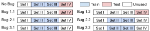
Figure 7: Example of training and testing data split.

Since previous architectures that are considered “bug-free” may actually have performance bugs, we also present results for the case when designs with a bug are presumed as “bug-free” and are used for training.

The results are shown in Table V. Although the same stage 2 classifier of our methodology is used, several different ML engines are used in stage 1 and listed in the “Stage 1 ML Model” column. The leftmost column indicates whether bug-free or “buggy” designs were used for training.

When only bug-free designs are used, using GBT-250 in stage 1 produces the best result. It can detect medium and high impact bugs ($>5\%$ IPC impact) with 98.5% true positive rate. When low impact bugs ($>1\%$ IPC impact) are additionally included, the true positive rate is still as high as $91.5\%$. The TPRs of GBT-250 beat the single-stage baseline in almost every bug category. It is also superior on ROC AUC. Meanwhile, it achieves 0 false-positive rate and 1.0 precision.

The table also shows two cases where the models were trained using designs with a bug. These two cases correspond to bugs with a low average IPC impact across the studied workloads. We included these as representative cases, and argue that bugs with higher IPC impact will most likely be caught during post-silicon validation of previous designs and will be fixed by the time a new microarchitecture is being developed. To evaluate these, we use GBT-250 model for stage 1 of the methodology as it was best performing. As expected, these results show some degradation in detection. However, GBT-250 is still able to detect around 70% of the bugs, while incurring a few false-positives.

In Figure 8 we show several examples of how the ROC curve looks for different bug types when stage 1 of our method uses GBT-250 model. Difficult to catch bugs usually have a lower ROC AUC, while other bugs with higher IPC impact can be detected without false-positives.

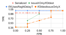
Figure 8: ROC curves for GBT-250 on different bug types.

V-C Number of Probes

There is a trade-off associated with the number of probes. More probes can potentially detect more bugs or reduce false positives, at the cost of higher runtime. To see how accuracy varies with probe count we examine the impact of reducing the number of probes. We perform this experiment in an iterative approach. Every iteration we remove five probes, re-train the model with the reduced set and collect its detection metrics. We evaluated these results using the GBT-250 model. We perform the probe reduction experiment with two different orders:

1. Remove the probes with the highest error in IPC inference first. The insight for using this method is, if a probe has high IPC inference error, it is likely that the model did not learn from it properly. The results are shown in Figure 9.

2. Remove probes in random order. This case is equivalent to having fewer probes with which to test the design. Results are shown in Figure 9.

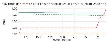
Figure 9: Effect of removing probes.

Results for both orderings, in Figure 9 show that, when the number of probes is reduced, the quality of results is degraded, either by an increase in FPR or by decreasing the TPR. It is also important to note, however, that the accuracy change is very slow versus probe reduction. Thus, our results are quite robust, arguing that even fewer benchmarks could be used as an input to the process with little impact on the outcome.

V-D Counter Selection

We evaluated our counter selection methodology by comparing with a set of 22 manually, but not arbitrarily, selected counters, which include miss rates for different cache levels, branch statistics and other counters related to the core pipeline and how many instructions each stage has processed. Unlike our method, we use the same 22 counters for all the probes. The results are evaluated for models 1-LSTM-500 and GBT-250. The obtained results can be seen on Figure 10.

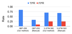
Figure 10: Effect of counter selection method.

Our counter selection methodology achieves better results in both machine learning models when compared to the results obtained by manually selecting the counters. Despite being heuristic, our counter selection methodology generally facilitates better detection results.

V-E Time Step Size

In stage 1 of IPC modelling, input features are taken as time series with each time step being 500K clock cycles. Experiments were performed to observe the effect of different time step sizes. The results are plotted in Figure 11. When the time step size increases, the inference errors for model 1-LSTM-500 decrease as shown in Figure 11(a). This is because coarser grained inference is generally easier than fine-grained. MSE is used here instead of the error defined by Eq. (1) as error area among different step sizes series are not comparable.

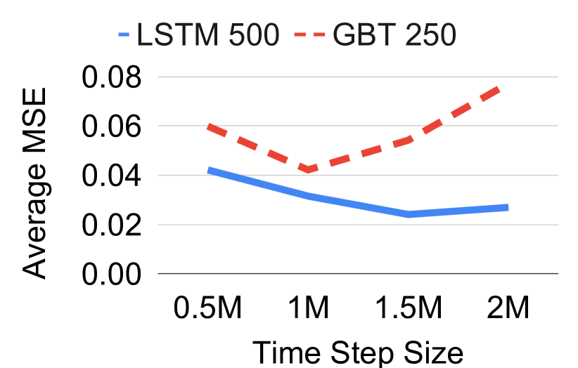
(a) Average MSE across all probes.

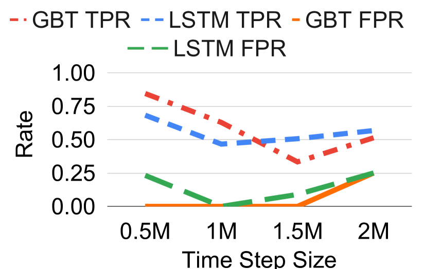
(b) TPR and FPR on bug detection.

Figure 11: Effect of different time step sizes.

The reduced IPC inference errors do not necessarily lead to improved bug detection results. In fact, Figure 11(b) shows that both TPR and FPR degrade as the time step size increases. The rationale is that whether or not the IPC inference is sensitive to bugs matters more than the accuracy. The results in Figure 11 confirm the choice of 500K cycles as the time step size. Besides the efficacy of bug detection, time step size also considerably affects computing runtime and data storage. In our experience, step size of 500K cycles reaches a good compromise between bug detection and computing load in our experiment setting.

V-F Window Size

The IPC inference in stage 1 can take the feature data from a series of time steps. So far in this paper, the window size we have used in our experiments has been one because the time step size is sufficiently large. Experiments were conducted to observe the impact of increasing the window size. Table VI shows the TPR and FPR obtained when the window size is increased for the model GBT-250.

TABLE VI: Window size effect.

	Window Size
	1	2	3	4
TPR	0.84	0.48	0.32	0.48
FPR	0.00	0.21	0.00	0.39

The results confirm the choice of a window size of one throughout our experiments. Given our time step size, the results suggest that adding information of previous time steps do not help to increase sensibility to performance bugs, furthermore, it actually degrades it.

V-G Microarchitecture Design Parameter Features

In our baseline methodology we propose the use of microarchitectural design parameters/specifications as static features (e.g. ROB size, issue width, etc.). Here, we examine the impact of removing these static features on the accuracy of our bug detection methodology. Figure 12 shows the obtained results.

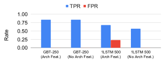
Figure 12: Effect of microarchitecture design parameter features.

The results show removing the design parameters has no impact on the accuracy of the GBT-250 model and a small reduction on the number of detected bugs with the 1LSTM-500 model, althought the number of false alarms is also reduced. This impact is contained within the bugs of Low or Very Low IPC impact. These results indicate that performance impact information is, in many cases, sufficiently contained within the performance counters (i.e. performance counter data inherently conveys enough information for the model to infer the IPC of different microarchitectures on the given workloads), and the change on microarchitectural specifications has a very small impact on the quality of results for our methodology.

V-H Number of training microarchitectures

We also evaluated the effect of reducing the number of available architectures to train our method. Here, we use 5 microarchitectures to train our IPC model (Set I), instead of 9. Sets II and III were reduced from 3 and 4 to 2 and 3 microarchitectures, respectively. In each case we dropped the “artificial” microarchitectures, keeping only the real ones. We keep the number of testing microarchitectures constant and show the results using GBT-250 in Figure 13.

From the obtained results we confirm that creating artificial architectures is necessary in order to augment our data set. This aids the model to learn the difference between performance variation due to microarchitectural specifications and performance bugs.

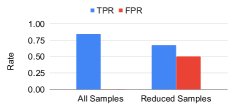
Figure 13: Effect of number of training microarchitectures.

V-I Bug Detection in Cache Memory Systems

In this section, we evaluate performance bug detection in the cache memory system, as described on Section IV-D. The obtained results are shown in Table VII.

TABLE VII: Bug detection in Memory Systems results.

					TPR for different bug categories
Stage 1 Metric	Stage 1 ML Model	FPR	TPR	Precision	High	Medium	Low	Very Low
IPC	LSTM	0.00	1.00	1.00	1.00	1.00	1.00	1.00
	GBT	0.00	1.00	1.00	1.00	1.00	1.00	1.00
AMAT	LSTM	0.00	0.82	1.00	1.00	1.00	1.00	0.20
	GBT	0.00	1.00	1.00	1.00	1.00	1.00	1.00

These results show that our methodology is able to detect all the bugs when GBT models are used for both IPC and AMAT inferences, while LSTM only misses Very Low AMAT impact bugs. The high accuracy of these results show that this methodology is robust for usage on different system components beyond the core, as well as different simulators.

VI Related Work

VI-A Microprocessor Performance Validation

The importance as well as the challenge of processor performance debug was recognized 26 years ago [9, 53]. However, the followup study has been scarce perhaps due to the difficulty. The few known works [9, 53, 55, 51, 46] generally follow the same strategy although with different emphasis. That is, an architecture model or an architecture performance model is constructed, and compared with the new design on a set of applications. Then, performance bugs can be detected if a performance discrepancy is observed in the comparison. In prior work by Bose [9], functional unit and instruction level models are developed as golden references. However, a performance bug often manifests in the interactions among different components or different instructions. Surya et al. [53] built an architecture timing model for PowerPC processor. It is focused on enforcing certain invariants in executing loops. For example, the IPC for executing a loop should not decrease when the buffer queue size increases. Although this technique is useful, its effectiveness is restricted to a few types of performance bugs. In work by Utamaphethai et al. [55], a microarchitecture design is partitioned into buffers, each of which is modeled by a finite state machine (FSM). Performance verification is carried out along with the functional verification using the FSM models. This method is effective only for state dependent performance bugs. The model comparison-based approach is also applied for the Intel Pentium 4 processor [51]. Similar approach is also applied for identifying I/O system performance anomaly [50]. A parametric machine learning model is developed for architecture performance evaluation [46]. This technique is mostly for guiding architecture design parameter (e.g., cache size) tuning.

Overall, the model comparison based approach has two main drawbacks. First, the same performance bug can appear in both the model and the design as described by Ho [26], and consequently cannot be detected. Although some works strive to find an accurate golden reference [9], such effort is restricted to special cases and very difficult to generalize. In particular, in presence of intrinsic performance variability [14, 52], finding golden reference for general cases becomes almost impossible. Second, constructing a reference architecture model is labor intensive and time consuming. On one hand, it is very difficult to build a general model applicable across different architectures. On the other hand, building one model for every new architecture is not cost-effective.

VI-B Performance Bugs in Other Domains

A related performance issue in datacenter computing is performance anomaly detection [29]. The main techniques here include statistics-based, such as ANOVA tests and regression analysis, and machine learning-based classification. Although there are many computers in a datacenter, the subject is the overall system performance upon workloads in very coarse-grained metrics. As such, the normal system performance is much better defined than individual processors. Performance bug detection is mentioned for distributed computing in clouds [33]. In this context, the overall computing runtime of a task is greater than the sum of runtimes of computing its individual component as extra time is needed for the data communication. However, the difference should be limited and otherwise an anomaly is detected. As such, the performance debug in distributed computing is focused on the communication and assumes that all processors are bug-free. Evidently, such assumption does not hold for processor microarchitecture designs. Gan et al. [22] developed an online QoS violation prediction technique for cloud computing. This technique applies runtime trace data to a machine learning model for the prediction and is similar to our baseline approach in certain extent. In another work, cloud service anomaly prediction is realized through self-organizing map, an unsupervised learning technique [15].

Performance bug is also studied for software systems where bugs are detected by users or code reasoning [43]. A machine learning approach is developed for evaluating software performance degradation due to code change [4]. Software code analysis [39] is used to identify performance critical regions when executing in cloud computing. Parallel program performance diagnosis is studied by Atachiants et al. [5]. Performance bugs in smartphone applications are categorized into a set of patterns [40] for future identification. As the degree of concurrency in microprocessor architectures is usually higher than a software program, performance debugging for microprocessor is generally much more complicated.

VI-C Performance Counters for Power Prediction

Prior work has used performance counters to predict power consumption [32, 13, 7, 57]. Joseph et al. [32] aim to predict average power consumption on complete workloads, as opposed to the time-series based strategy we use for accurate detection of bugs. Counters are selected based on heuristics, without automation. Contreras  et al. [13] further improves this work and present an automated performance counter selection technique able to do time-series prediction of the power. However, this technique was evaluated on an Intel PXA255 processor, a single-issue machine, making the problem much simpler than aiming at super-scalar processors. Bircher et al. [7] further improves this line of work by creating models other units, such as memory, disk and interconnect. The main drawback of this work is that it requires a thorough study of the design characteristics in order to create the performance counter list to be used. Recent work by Yang et al. [57] further expanded Bircher’s work by aiming to develop a full system power model, prior work had only focused on component based modeling.

Although this line of work has similarities with our IPC estimation methodology, our work is the first whose goal is the identification of performance bugs in a design. Further, because our goal is performance bug detection via orthogonal probes, we can make our models orthogonal and specific to each probe, thus we achieve very high IPC estimation accuracy, higher than is possible with the generalized models needed for general power prediction/management. Another significant difference is that our methodology is able to generalize to multiple microarchitectures, whereas the methodologies discussed in this section are trained and tested on the same processor.

VII Conclusion and Future Work

In this work, a machine learning-based approach to automatic performance bug detection is developed for processor core microarchitecture designs. The machine learning models extract knowledge from legacy designs and avoid the previous methods of reference performance models, which are error prone and time consuming to construct. Simulation results show that our methodology can detect 91.5% of the bugs with impact greater than 1% of the IPC on a new microarchitecture when completely new bugs exist in a new microarchitecture. With this study we also hope to draw the attention of the research community to the broader performance validation domain.

In future research, we will extend the methodology for debugging of multi-core memory systems and on-chip communication fabrics. We will also further study how to automatically narrow down bug locations once they are detected. As in functional debug [41], the results from our method will potentially serve as symptoms for bug localization. By analyzing characteristics in common across the probes triggering the bug detection (e.g. most common instruction types, memory or computational boundness, etc), the designers could reduce the list of potential bug locations. Another debugging path could be the analysis of the counters selected for the IPC inference models of those traces. Factors such as a lost of correlation between the counters and IPC when compared to legacy designs could also help to pinpoint possible sources of bug.

References

- [1] “ChampSim: A trace based microarchitecture simulator,” https://github.com/ChampSim/ChampSim.
- [2] “SPEC CPU2006,” https://www.spec.org/cpu2006.
- [3] “SPEC CPU2017,” https://www.spec.org/cpu2017.
- [4] M. Alam, J. Gottschlich, N. Tatbul, J. S. Turek, T. Mattson, and A. Muzahid, “A zero-positive learning approach for diagnosing software performance regressions,” in Advances in Neural Information Processing Systems, 2019, pp. 11 623–11 635.
- [5] R. Atachiants, G. Doherty, and D. Gregg, “Parallel performance problems on shared-memory multicore systems: taxonomy and observation,” in IEEE Transactions on Software Engineering, vol. 42, no. 8, 2016, pp. 764–785.
- [6] N. Binkert, B. Beckmann, G. Black, S. K. Reinhardt, A. Saidi, A. Basu, J. Hestness, D. R. Hower, T. Krishna, S. Sardashti, R. Sen, K. Sewell, M. Shoaib, N. Vaish, M. D. Hill, and D. A. Wood, “The Gem5 simulator,” in SIGARCH Computer Architecture News, vol. 39, no. 2, 2011, pp. 1–7.
- [7] W. L. Bircher and L. K. John, “Complete system power estimation: A trickle-down approach based on performance events,” in IEEE International Symposium on Performance Analysis of Systems Software, 2007, pp. 158–168.
- [8] B. Black, A. S. Huang, M. H. Lipasti, and J. P. Shen, “Can trace-driven simulators accurately predict superscalar performance?” in International Conference on Computer Design. VLSI in Computers and Processors, 1996, pp. 478–485.
- [9] P. Bose, “Architectural timing verification and test for super scalar processors,” in IEEE International Symposium on Fault-Tolerant Computing, 1994, pp. 256–265.
- [10] T. Chen and C. Guestrin, “XGBoost: A scalable tree boosting system,” in ACM SIGKDD International Conference on Knowledge Discovery and Data Mining, 2016, pp. 785–794.
- [11] F. Chollet, “Keras,” https://keras.io, 2015.
- [12] T. M. Conte, M. A. Hirsch, and K. N. Menezes, “Reducing state loss for effective trace sampling of superscalar processors,” in International Conference on Computer Design. VLSI in Computers and Processors, 1996, pp. 468–477.
- [13] G. Contreras and M. Martonosi, “Power prediction for Intel XScale processors using performance monitoring unit events,” in International Symposium on Low Power Electronics and Design, 2005, pp. 221–226.
- [14] B. Cook, T. Kurth, B. Austin, S. Williams, and J. Deslippe, “Performance variability on Xeon Phi,” in International Conference on High Performance Computing, 2017, pp. 419–429.
- [15] D. J. Dean, H. Nguyen, and X. Gu, “UBL: Unsupervised behavior learning for predicting performance anomalies in virtualized cloud systems,” in International Conference on Autonomic Computing, 2012, pp. 191–200.
- [16] C. Delimitrou and C. Kozyrakis, “iBench: Quantifying interference for datacenter applications,” in IEEE International Symposium on Workload Characterization, 2013, pp. 23–33.
- [17] C. Delimitrou, D. Sanchez, and C. Kozyrakis, “Tarcil: Reconciling scheduling speed and quality in large shared clusters,” in ACM Symposium on Cloud Computing, 2015, pp. 97–110.
- [18] R. Desikan, D. Burger, and S. W. Keckler, “Measuring experimental error in microprocessor simulation,” in International Symposium on Computer Architecture, 2001, p. 266–277.
- [19] J. Doweck, W.-F. Kao, A. K.-y. Lu, J. Mandelblat, A. Rahatekar, L. Rappoport, E. Rotem, A. Yasin, and A. Yoaz, “Inside 6th-generation Intel Core: New microarchitecture code-named Skylake,” in IEEE Micro, vol. 37, no. 2, 2017, pp. 52–62.
- [20] L. Eren, T. Ince, and S. Kiranyaz, “A generic intelligent bearing fault diagnosis system using compact adaptive 1D CNN classifier,” in Journal of Signal Processing Systems, vol. 91, no. 2, 2019, pp. 179–189.
- [21] J. H. Friedman, “Greedy function approximation: a gradient boosting machine,” in Annals of Statistics, 2001, pp. 1189–1232.
- [22] Y. Gan, Y. Zhang, K. Hu, D. Cheng, Y. He, M. Pancholi, and C. Delimitrou, “Seer: Leveraging big data to navigate the complexity of performance debugging in cloud microservices,” in International Conference on Architectural Support for Programming Languages and Operating Systems, 2019, pp. 19–33.
- [23] P. Gepner, D. L. Fraser, and V. Gamayunov, “Evaluation of the 3rd generation Intel Core processor focusing on HPC applications,” in International Conference on Parallel and Distributed Processing Techniques and Applications, 2012, pp. 1–6.
- [24] G. Hamerly, E. Perelman, and B. Calder, “How to use simpoint to pick simulation points,” in ACM SIGMETRICS Performance Evaluation Review, vol. 31, no. 4, 2004, pp. 25–30.
- [25] G. Hamerly, E. Perelman, J. Lau, and B. Calder, “Simpoint 3.0: Faster and more flexible program phase analysis,” in Journal of Instruction Level Parallelism, vol. 7, no. 4, 2005, pp. 1–28.
- [26] R. C. Ho, C. H. Yang, M. A. Horowitz, and D. L. Dill, “Architecture validation for processors,” in International Symposium on Computer Architecture, 1995, pp. 404–413.
- [27] S. Hochreiter and J. Schmidhuber, “Long short-term memory,” in Neural Computation, vol. 9, no. 8, 1997, pp. 1735–1780.
- [28] K. Hornik, M. Stinchcombe, and H. White, “Multilayer feedforward networks are universal approximators,” in Neural Networks, vol. 2, no. 5, 1989, pp. 359 – 366.
- [29] O. Ibidunmoye, F. Hernández-Rodriguez, and E. Elmroth, “Performance anomaly detection and bottleneck identification,” in ACM Computing Surveys, vol. 48, no. 1, 2015, pp. 1–35.
- [30] Intel Corporation, “Intel386™ DX processor: Specification update,” 2004.
- [31] Intel Corporation, “Intel Xeon processor scalable family: Specification update,” 2019.
- [32] R. Joseph and M. Martonosi, “Run-time power estimation in high performance microprocessors,” in International Symposium on Low power electronics and design, 2001, pp. 135–140.
- [33] C. Killian, K. Nagaraj, S. Pervez, R. Braud, J. W. Anderson, and R. Jhala, “Finding latent performance bugs in systems implementations,” in ACM SIGSOFT International Symposium on Foundations of Software Engineering, 2010, pp. 17–26.
- [34] J. Kim, S. H. Pugsley, P. V. Gratz, A. N. Reddy, C. Wilkerson, and Z. Chishti, “Path confidence based lookahead prefetching,” in International Symposium on Microarchitecture, 2016, pp. 1–12.
- [35] D. P. Kingma and J. Ba, “Adam: A method for stochastic optimization,” in International Conference for Learning Representations, 2015.
- [36] Y. LeCun and Y. Bengio, “Convolutional networks for images, speech, and time series,” in The handbook of brain theory and neural networks, 1995.
- [37] S.-M. Lee, S. M. Yoon, and H. Cho, “Human activity recognition from accelerometer data using convolutional neural network,” in IEEE International Conference on Big Data and Smart Computing, 2017, pp. 131–134.
- [38] J. Leverich and C. Kozyrakis, “Reconciling high server utilization and sub-millisecond quality-of-service,” in European Conference on Computer Systems, 2014, pp. 1–14.
- [39] J. Li, Y. Chen, H. Liu, S. Lu, Y. Zhang, H. S. Gunawi, X. Gu, X. Lu, and D. Li, “Pcatch: Automatically detecting performance cascading bugs in cloud systems,” in EuroSys Conference, 2018, pp. 1–14.
- [40] Y. Liu, C. Xu, and S.-C. Cheung, “Characterizing and detecting performance bugs for smartphone applications,” in International Conference on Software Engineering, 2014, pp. 1013–1024.
- [41] B. Mammo, M. Furia, V. Bertacco, S. Mahlke, and D. S. Khudia, “Bugmd: Automatic mismatch diagnosis for bug triaging,” in International Conference on Computer-Aided Design, 2016, pp. 1–7.
- [42] J. D. McCalpin, “HPL and DGEMM performance variability on the Xeon platinum 8160 processor,” in International Conference for High Performance Computing, Networking, Storage and Analysis, 2018, pp. 225–237.
- [43] A. Nistor, T. Jiang, and L. Tan, “Discovering, reporting, and fixing performance bugs,” in Working Conference on Mining Software Repositories, 2013, pp. 237–246.
- [44] T. Nowatzki, J. Menon, C. Ho, and K. Sankaralingam, “Architectural simulators considered harmful,” in IEEE Micro, vol. 35, no. 6, 2015, pp. 4–12.
- [45] NXP Semicondutctors, “Chip errata for the MPC7448,” 2008.
- [46] E. Ould-Ahmed-Vall, J. Woodlee, C. Yount, K. A. Doshi, and S. Abraham, “Using model trees for computer architecture performance analysis of software applications,” in IEEE International Symposium on Performance Analysis of Systems & Software, 2007, pp. 116–125.
- [47] F. Pedregosa, G. Varoquaux, A. Gramfort, V. Michel, B. Thirion, O. Grisel, M. Blondel, P. Prettenhofer, R. Weiss, V. Dubourg, J. Vanderplas, A. Passos, D. Cournapeau, M. Brucher, M. Perrot, and E. Duchesnay, “Scikit-learn: Machine learning in Python,” Journal of Machine Learning Research, vol. 12, pp. 2825–2830, 2011.
- [48] E. Perelman, G. Hamerly, M. Van Biesbrouck, T. Sherwood, and B. Calder, “Using simpoint for accurate and efficient simulation,” in ACM SIGMETRICS Performance Evaluation Review, vol. 31, no. 1, 2003, pp. 318–319.
- [49] F. Santosa and W. Symes, “Linear inversion of band-limited reflection seismograms,” in SIAM Journal on Scientific and Statistical Computing, vol. 7, no. 4, 1986, pp. 1307–1330.
- [50] K. Shen, M. Zhong, and C. Li, “I/O system performance debugging using model-driven anomaly characterization.” in USENIX Conference on File and Storage Technologies, vol. 5, 2005, pp. 309–322.
- [51] R. Singhal, K. Venkatraman, E. R. Cohn, J. G. Holm, D. A. Koufaty, M.-J. Lin, M. J. Madhav, M. Mattwandel, N. Nidhi, J. D. Pearce et al., “Performance analysis and validation of the Intel® Pentium® 4 processor on 90nm technology.” in Intel Technology Journal, vol. 8, no. 1, 2004, pp. 39–48.
- [52] D. Skinner and W. Kramer, “Understanding the causes of performance variability in HPC workloads,” in IEEE Workload Characterization Symposium, 2005, pp. 137–149.
- [53] S. Surya, P. Bose, and J. Abraham, “Architectural performance verification: PowerPC processors,” in IEEE International Conference on Computer Design: VLSI in Computers and Processors, 1994, pp. 344–347.
- [54] Texas Instruments, “AM3517, AM3505 Sitara processors silicon revisions 1.1, 1.0: Silicon errata,” 2016.
- [55] N. Utamaphethai, R. S. Blanton, and J. P. Shen, “A buffer-oriented methodology for microarchitecture validation,” in Journal of Electronic Testing, vol. 16, no. 1-2, 2000, pp. 49–65.
- [56] R. E. Wunderlich, T. F. Wenisch, B. Falsafi, and J. C. Hoe, “SMARTS: Accelerating microarchitecture simulation via rigorous statistical sampling,” in International Symposium on Computer Architecture, 2003, pp. 84–97.
- [57] S. Yang, Z. Luan, B. Li, G. Zhang, T. Huang, and D. Qian, “Performance events based full system estimation on application power consumption,” in International Conference on High Performance Computing and Communications, 2016, pp. 749–756.