Calculus of variations rationalises long-wavelength flagellar waves

Hydrodynamically optimal long-wavelength flagella have constant-speed travelling waves

Using calculus of variations to rationalise long-wavelength flagellar waves

Hydrodynamically optimal long-wavelength flagella deform as travelling waves

Travelling waves are hydrodynamically optimal for long-wavelength flagella

Abstract

Swimming eukaryotic microorganisms such as spermatozoa, algae and ciliates self-propel in viscous fluids using travelling wave-like deformations of slender appendages called flagella. Waves are predominant because Purcell’s scallop theorem precludes time-reversible kinematics for locomotion. Using the calculus of variations on a periodic long-wavelength model of flagellar swimming, we show that the planar flagellar kinematics maximising the time-averaged propulsive force for a fixed amount of energy dissipated in the surrounding fluid correspond for all times to waves travelling with constant speed, potentially on a curved centreline, with propulsion always in the direction opposite to the wave.

I Introduction

A large proportion of all micro-organisms are able to self-propel in liquids, including spermatozoa, algae, ciliates and many species of bacteria yates86 . In order to achieve self-propulsion, most cells exploit flagella – slender whiplike organelles extending out of the cell body and whose time-varying deformations powered by molecular motors induces flows and creates the propulsive forces required to overcome viscous friction braybook . Due to their small sizes and speeds, swimming cells move at low Reynolds number, a regime which is qualitatively different from the high-Reynolds world of fish and birds, and with well-studied physical consequences childress81 . A lot of work has been devoted by the scientific community to uncover the physical principles behind the dynamics of individual cells and to capture their interactions in complex environments gray68 ; lighthill75 ; lighthill76 ; brennen77 ; lp09 .

Despite the tremendous variation in size, geometry, kinematics, ecosystems and evolutionary position on the tree of life, one universal feature of swimming cells is the use of waves to induce locomotion. The physical rationale for the appearance of travelling waves lies in Purcell’s famed scallop theorem, which states that the time-reversible motion of a swimmer can never produce locomotion purcell77 . Therefore, biological swimmers need to deform in a manner that indicates a clear direction of time, the prototypical example of which is a wave. Bacteria use helical semi-rigid filaments, each of which is rotated by a specialised rotary motor leading to apparent longitudinal waves of displacement berg00_PT . The physics of helical propulsion is now well understood lauga16 , including the fact that the flagellar shapes observed in bacteria are close to that of the optimal propeller predicted by theory spagnolie2011 .

Swimming eukaryotic cells (i.e. biological cells with a nucleus, in contrast with bacteria) also use flagellar waves in order to self-propel. Unlike bacteria, the flagella of eukaryotes are flexible, active filaments that deform with travelling wave-like motion, in most cases planar. While a bacterial flagellum is passively rotated by a single motor, the actuation of eukaryotes is spatially distributed inside the flagellum and it involves the coordinated action of a large number of molecular motors julicher1997modeling . The model organisms from which we have learnt the most include (i) spermatozoa, mostly of invertebrates and mammals fauci06 ; gaffney11 ; (ii) single cells such as the algal genus Chlamydomonas equipped with a pair of flagella pedley92 ; stocker or ciliates, e.g. the genus Paramecium blake74 ; brennen77 ; and (iii) multicellular organisms such as the algal genus Volvox powered by a large number of short flagella goldstein:15 .

All these organisms have in common that their swimming is propelled by travelling wave-like motion of their flagella. Such a simple observation within such a wide biological spectrum has invariably lead the scientific community to look for flagellar waving as the solution to an optimisation problem. The most formal result was obtained by Pironneau and Katz using the calculus of variations pironneau74 , a well known mathematical framework to address problems in shape optimisation, with broad applications in fluid mechanics at both high mohammadi2004shape and low Reynolds numbers pironneau1974optimum ; montenegro2015other . In their paper, Pironneau and Katz considered organisms with no cell body swimming using the two-dimensional waving of a slender flagellum. Using the resistive-force theory of slender filaments, they showed that the kinematics of the deforming flagellum that lead to locomotion with the least amount of energy dissipated in the surrounding fluid, subject to a fixed constraint of local flagellum velocity projected on the tangent of the flagellum and spatially-averaged, correspond in the swimming frame to an apparent sliding of the flagellum along its instantaneous centreline. This suggested flagellar waves travelling instantaneously in the direction opposite to that of the locomotion pironneau74 .

This energetic advantage of flagellar waves encouraged the scientific community to then hunt for the optimal wave. In two dimensions, the hydrodynamically optimal waving sheet has to be characterised numerically and takes the form of a front-back symmetric regularised cusp montenegro2014optimal . For a slender filament, the optimal wave has a constant angle between the local tangent to the filament and the direction of wave propagation taking therefore the shape of a helix for three-dimensional motion and straight segments joined in kinks for planar flagellar waves pironneau74 ; pironneau_inbook ; lighthill75 . This kink can be regularised by taking into account the elastic cost of bending the flagellum Spagnolie2010 or the irreversible nature of the internal rate of working of the molecular motors powering the flagellum laugaeloy13 . Optimal waving motion has also been investigated for biflagellate algae tam2011optimal , simple swimmers with small numbers of degrees of freedom tam07 and coordinated waving in the locomotion and feeding of ciliates michelin2010 ; michelin2011 ; osterman2011finding ; eloylauga12 ; michelin2013 . More formal mathematical approaches to the optimisation problem have also been developed avron04:opt ; alouges08 ; AlougesDeSimoneLefebvre2009 . Recently, reinforcement learning has been proposed as a mechanism to help design favourable swimming strokes for simple artificial swimmers tsang2020self .

In this paper, we show that a simple calculation using the tools of the calculus of variations allows to rationalise analytically the predominance of constant-speed flagellar waves for long-wavelength motion. Assuming planar motion, we mathematically determine the flagellar kinematics maximising the time-averaged propulsive force for a fixed amount of total energy dissipated in the surrounding fluid. We show that they correspond, for all times, to waves travelling with constant speed, potentially on a curved flagellum centreline, and always lead to propulsion in the direction opposite to that of the wave.

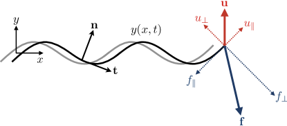
Figure 1: An infinite flexible flagellum undergoing planar beating is described mathematically by a time-varying function $y(x,t)$ in Cartesian coordinates. The unit vectors ${\bf t}$ and ${\bf n}$ are the local tangent and normal to the instantaneous flagellar shape. The instantaneous velocity of the flagellum centreline, ${\bf u}$, can be decomposed into components along the directions tangent ($u_{\parallel}$) and normal to the flagellum ($u_{\perp}$), and similarly for the hydrodynamic force density acting on the flagellum, ${\bf f}$ (components $f_{\parallel}$ and $f_{\perp}$). The force and velocity components are related to one another through resistive-force theory. We use the calculus of variations to determine the class of functions $y(x,t)$ leading to the maximal average propulsive force for a given amount of average energy dissipated in the fluid.

II Propulsion and energetics of a deforming flagellum

II.1 Setup

Locomotion is induced in a Newtonian fluid by the planar deformation of a flexible inextensible flagellum (setup in Fig. 1). The shape of the flagellum is described in Cartesian coordinates by material points $\big{(}x,y(x,t)\big{)}$, and the flagellum is assumed to be infinite and slender. We focus on the limit of long-wavelength motion and therefore we assume $|{\partial}y/{\partial}x|\ll 1$ everywhere. The flagellum is spatially-periodic with fixed period $\lambda$ in the $x$ direction and the deformations are periodic in time with fixed period $T$.

II.2 Propulsive force

We first compute the propulsive force generated by the deforming flagellum, i.e. the net hydrodynamic force experienced by the total flagellum along the swimming direction (assumed to be $x$) and resulting from its time-varying motion. Denoting by ${\bf u}$ the velocity of the flagellum centreline relative to the background fluid, we use the resistive-force theory of viscous hydrodynamics, an asymptotic result valid in the limit of slender filaments, to compute the hydrodynamic forces acting on the filament in the limit of low Reynolds number cox70 ; batchelor70 .

In this limit, the local hydrodynamic force per unit length along the filament, ${\bf f}$, is decomposed into its component parallel to the local unit tangent vector ${\bf t}$, ${\bf f}_{\parallel}=({\bf f}\cdot{\bf t}){\bf t}$, and its perpendicular component, ${\bf f}_{\perp}={\bf f}-{\bf f}_{\parallel}=({\bf f}\cdot{\bf n}){\bf n}$, where ${\bf n}$ is the unit normal to the flagellum chosen so that ${\bf t}\times{\bf n}={\bf e}_{z}$. The magnitudes of these two force components are

$$f_{\parallel}=-c_{\parallel}u_{\parallel},\quad f_{\perp}=-c_{\perp}u_{\perp},$$ (1)

where $u_{\parallel}$ and $u_{\perp}$ are the local components of the flagellum velocity parallel and perpendicular to the local tangent (see sketch in Fig. 1). In Eq. (1), the parameters $c_{\parallel}$ and $c_{\perp}$ are the perpendicular and parallel drag coefficients, given in the slender limit $a\ll L$ by $c_{\perp}\approx 2c_{\parallel}\approx 4\pi\mu/\ln(L/a)$ where $a$ is the cross sectional radius of the flagellum and $L$ is either its length if the flagellum is finite cox70 ; batchelor70 or a characteristic length proportional to the wavelength if it is infinite lighthill75 .

The two components in Eq. (1) can be combined to obtain an equation relating the hydrodynamic force density vector, ${\bf f}$, to the local filament velocity vector, ${\bf u}$, as

$${\bf f}=-[c_{\parallel}{\bf t}{\bf t}+c_{\perp}{\bf n}{\bf n}]\cdot{\bf u}.$$ (2)

The $x$-component of the time-averaged propulsive force, denoted by $F_{x}$, is then given as a double integral over the period and the wavelength

$$F_{x}=\frac{1}{T}\int_{0}^{T}\int_{0}^{\lambda}{\bf f}\cdot{\bf e}_{x}\,\,{\rm d}x\,{\rm d}t,$$ (3)

which, given Eq. (2), is equal to

$$F_{x}=-\frac{1}{T}\int_{0}^{T}\int_{0}^{\lambda}[c_{\parallel}({\bf t}\cdot{\bf e}_{x})({\bf u}\cdot{\bf t})+c_{\perp}({\bf n}\cdot{\bf e}_{x})({\bf u}\cdot{\bf n})]\,{\rm d}x\,{\rm d}t.$$ (4)

In the case of a flagellum where $|{\partial}y/{\partial}x|\ll 1$, we have the leading-order long-wavelength geometry and velocity given by

$${\bf t}=\left(\begin{array}[]{c}1\\ \displaystyle\frac{{\partial}y}{{\partial}x}\end{array}\right),\quad{\bf n}=\left(\begin{array}[]{c}\displaystyle-\frac{{\partial}y}{{\partial}x}\\ 1\end{array}\right),\quad{\bf u}=\left(\begin{array}[]{c}0\\ \displaystyle\frac{{\partial}y}{{\partial}t}\end{array}\right),$$ (5)

so that

$${\bf u}\cdot{\bf t}=\frac{{\partial}y}{{\partial}x}\frac{{\partial}y}{{\partial}t},\quad{\bf u}\cdot{\bf n}=\frac{{\partial}y}{{\partial}t},$$ (6)

and thus the integrand in Eq. (3) becomes

$${\bf f}\cdot{\bf e}_{x}=(c_{\perp}-c_{\parallel})\frac{{\partial}y}{{\partial}x}\frac{{\partial}y}{{\partial}t},$$ (7)

at leading order in the long wavelength limit.

Integrating in space over one wavelength and calculating the average in time leads to the mean propulsive force as

$$F_{x}=\frac{(c_{\perp}-c_{\parallel})}{T}\int_{0}^{T}\int_{0}^{\lambda}\frac{{\partial}y}{{\partial}t}\frac{{\partial}y}{{\partial}x}\,{\rm d}x\,{\rm d}t.$$ (8)

We now wish to determine the function $y(x,t)$ of both time and space that maximises the propulsive force in Eq. (8) for a given amount of energy expended by the flagellum. In the long-wavelength approximation, the drag per unit length exerted on a flagellum translating with speed $U$ is equal to $-c_{\parallel}U$ at leading order. Hence the swimming speed of the flagellum in Stokes flow is directly proportional to the propulsive force with a coefficient of proportionality independent of the shape; maximising $F_{x}$ is thus equivalent to maximising $U$.

II.3 Flagellum energetics

We next make the standard assumption that the majority of the energy expended by the flagellum is dissipated in the surrounding viscous fluid lighthill76 , and thus neglect internal sources of dissipation. The rate of energy dissipation in the fluid is equal to the rate of working (or power) of the moving flagellum against the fluid. Since ${\bf f}$ is the hydrodynamic force per unit length acting on the filament, the power density is $\dot{w}=-{\bf f}\cdot{\bf u}$, which we then need to integrate over the whole length of the flagellum. Given Eq. (2), we have

$$\dot{w}=c_{\perp}({\bf u}\cdot{\bf n})^{2}+c_{\parallel}({\bf u}\cdot{\bf t})^{2}.$$ (9)

Using the results of Eq. (5), we see that the leading-order value of the power density is given by

$$\dot{w}=c_{\perp}\left(\frac{{\partial}y}{{\partial}t}\right)^{2},$$ (10)

plus small corrections in the long-wavelength limit. The leading-order time-averaged rate of working of the flagellum over one wavelength, $\dot{W}$, is therefore given by the double integration in time and over a wavelength as

$$\dot{W}=\frac{c_{\perp}}{T}\int_{0}^{T}\int_{0}^{\lambda}\left(\frac{{\partial}y}{{\partial}t}\right)^{2}\,{\rm d}x\,{\rm d}t.$$ (11)

Notably, we see that the dissipation is dominated at leading order by the lateral motion of the flagellum.

III Hydrodynamically optimal active flagellum

III.1 Optimisation setup

We wish to determine the time-varying shape of the periodic flagellum that maximises the value of $F_{x}$ (Eq. 8) for a given value of $\dot{W}$ (Eq. 11). For this optimisation problem we define the Lagrangian

$${\cal L}[y]\equiv F_{x}+\Gamma(\dot{W}-\dot{W}_{0}),$$ (12)

where $\Gamma$ is a constant Lagrange multiplier and the constant $\dot{W}_{0}$ is the value of the constraint for $\dot{W}$. By considering a small periodic change in the shape of the flagellum, $y\to y+\delta y$, we now calculate the resulting change in the functional, ${\cal L}\to{\cal L}+\delta{\cal L}$. We will then ask what time-varying flagellum shape renders the first functional derivative zero, i.e. $\delta{\cal L}=0$. Throughout we assume that the flagellum is periodic in space with wavelength $\lambda$ and periodic in time with period $T$, both of which are constant, so that we require

$$y(x+\lambda,t)=y(x,t),\quad y(x,t+T)=y(x,t).$$ (13)

III.2 Calculus of variations

To compute the change in ${\cal L}$ we write $\delta{\cal L}=\delta F_{x}+\Gamma\delta\dot{W}$ and calculate each term separately.

III.2.1 Variation of the propulsive force

Since the propulsive force is quadratic in the flagellum shape and its velocity, a perturbation of Eq. (8) leads to

$$\delta F_{x}=\frac{(c_{\perp}-c_{\parallel})}{T}\int_{0}^{T}\int_{0}^{\lambda}\left(\frac{{\partial}y}{{\partial}t}\frac{{\partial}\delta y}{{\partial}x}+\frac{{\partial}\delta y}{{\partial}t}\frac{{\partial}y}{{\partial}x}\right)\,{\rm d}x\,{\rm d}t.$$ (14)

We then use integration by parts to evaluate each term. For the first one we write

$$\int_{0}^{T}\int_{0}^{\lambda}\frac{{\partial}y}{{\partial}t}\frac{{\partial}\delta y}{{\partial}x}\,{\rm d}x\,{\rm d}t=\int_{0}^{T}\int_{0}^{\lambda}\frac{{\partial}}{{\partial}x}\left(\frac{{\partial}y}{{\partial}t}\delta y\right)\,{\rm d}x\,{\rm d}t$$

$$-\int_{0}^{T}\int_{0}^{\lambda}\delta y\frac{{\partial}^{2}y}{{\partial}t{\partial}x}\,{\rm d}x\,{\rm d}t.$$ (15)

The spatial integral of the term $\frac{{\partial}}{{\partial}x}\left(\frac{{\partial}y}{{\partial}t}\delta y\right)$ is zero by spatial periodicity of the flagellum velocity and its perturbation, and thus

$$\int_{0}^{T}\int_{0}^{\lambda}\frac{{\partial}y}{{\partial}t}\frac{{\partial}\delta y}{{\partial}x}\,{\rm d}x\,{\rm d}t=-\int_{0}^{T}\int_{0}^{\lambda}\delta y\frac{{\partial}^{2}y}{{\partial}t{\partial}x}\,{\rm d}x\,{\rm d}t.$$ (16)

The same manipulation can be carried out for the second term on the right-hand side of Eq. (III.2.1) and we find

$$\int_{0}^{T}\int_{0}^{\lambda}\frac{{\partial}y}{{\partial}x}\frac{{\partial}\delta y}{{\partial}t}\,{\rm d}x\,{\rm d}t=\int_{0}^{T}\int_{0}^{\lambda}\frac{{\partial}}{{\partial}t}\left(\frac{{\partial}y}{{\partial}x}\delta y\right)\,{\rm d}x\,{\rm d}t$$

$$-\int_{0}^{T}\int_{0}^{\lambda}\delta y\frac{{\partial}^{2}y}{{\partial}t{\partial}x}\,{\rm d}x\,{\rm d}t,$$ (17)

and this time the first integral on the right-hand side is zero by periodicity in time of the flagellum and its perturbation. We therefore obtain the final result for the variation of the force

$$\delta F_{x}=\frac{2(c_{\parallel}-c_{\perp})}{T}\int_{0}^{T}\int_{0}^{\lambda}\delta y\frac{{\partial}^{2}y}{{\partial}t{\partial}x}\,{\rm d}x\,{\rm d}t.$$ (18)

III.2.2 Variation of the rate of working

The perturbation of the expression for the rate of working is dealt with similarly. Here, again, we have a quadratic quantity, so perturbing Eq. (11) leads to

$$\delta W=\frac{2c_{\perp}}{T}\int_{0}^{T}\int_{0}^{\lambda}\frac{{\partial}y}{{\partial}t}\frac{{\partial}\delta y}{{\partial}t}\,{\rm d}x\,{\rm d}t.$$ (19)

Using an integration by parts in time and invoking again periodicity in time we obtain

$$\delta W=-\frac{2c_{\perp}}{T}\int_{0}^{T}\int_{0}^{\lambda}\frac{{\partial}^{2}y}{{\partial}t^{2}}\delta y\,{\rm d}x\,{\rm d}t.$$ (20)

III.2.3 Optimal waveform

Given Eqs. (18) and (20), we obtain the variation in the Lagrangian as

$$\delta{\cal L}=\frac{2}{T}\int_{0}^{T}\int_{0}^{\lambda}\delta y\left[(c_{\parallel}-c_{\perp})\frac{{\partial}^{2}y}{{\partial}t{\partial}x}-\Gamma c_{\perp}\frac{{\partial}^{2}y}{{\partial}t^{2}}\right]\,{\rm d}x\,{\rm d}t.$$ (21)

The standard first-order optimality condition is $\delta{\cal L}=0$ for all perturbations $\delta y$ and therefore the waveform shape is governed by the partial differential equation

$$\Gamma c_{\perp}\frac{{\partial}^{2}y}{{\partial}t^{2}}=(c_{\parallel}-c_{\perp})\frac{{\partial}^{2}y}{{\partial}t{\partial}x}\cdot$$ (22)

This equation can be integrated in time once to obtain

$$\Gamma c_{\perp}\frac{{\partial}y}{{\partial}t}=(c_{\parallel}-c_{\perp})\frac{{\partial}y}{{\partial}x}+A(x),$$ (23)

where $A(x)$ is an arbitrary periodic function. To simplify notation we write this function as $A(x)\equiv(c_{\perp}-c_{\parallel}){\cal H}^{\prime}(x)$ so that the optimality condition in Eq. (23) may be rewritten as

$$\Gamma c_{\perp}\frac{{\partial}y}{{\partial}t}=(c_{\parallel}-c_{\perp})\left(\frac{{\partial}y}{{\partial}x}-{\cal H}^{\prime}(x)\right).$$ (24)

We next define the new variable $z(x,t)\equiv y(x,t)-{\cal H}(x)$, for which we obtain a transport equation

$$\frac{{\partial}z}{{\partial}t}=\frac{(c_{\parallel}-c_{\perp})}{\Gamma c_{\perp}}\frac{{\partial}z}{{\partial}x}.$$ (25)

The solutions to Eq. (25) are waves travelling with constant speed. The energetically-optimal solution breaks therefore the right-left symmetry of the problem, recovering what was postulated phenomenologically for active filaments goldstein2016elastohydrodynamic . As a consequence, the general solution for the flagellum waveform $y(x,t)$ is given by

$$y(x,t)={\cal H}(x)+{\cal Y}\left[x-\frac{(c_{\perp}-c_{\parallel})}{\Gamma c_{\perp}}t\right],$$ (26)

with both $\cal H$ and $\cal Y$ periodic functions of period $\lambda$. Importantly, these long-wavelength functions are arbitrary, provided that they satisfy the periodicity (Sec. III.2.4) and energy constraints (Sec. III.2.5). The flagellar kinematics maximising the mean propulsive force $F_{x}$ for a fixed value of energy dissipated in the fluid $\dot{W}_{0}$ are therefore travelling waves; the function $\cal H$ represents the average shape of the flagellum centreline, and $\cal Y$ the shape of the travelling wave around this average. In nature, many flagellated species have shapes that oscillate periodically around a straight configuration and correspond to the case ${\cal H}=0$ brennen77 . Some organisms however have a non-straight centreline, for example the spermatozoa of chinchilla woolley03 , bull friedrich2010high and some insects pak2012hydrodynamics , all of which would correspond to the case where ${\cal H}\neq 0$.

III.2.4 Lagrange multiplier

The value of the Lagrange multiplier is obtained as a consequence of the periodicity of the waveform. Since $y(x,t)$ satisfies the spatio-temporal periodicity from Eq. (13), for the function $\cal Y$ of a travelling-wave argument in Eq. (26) to follow the same periodicity it is necessary that

$$\frac{(c_{\perp}-c_{\parallel})}{\Gamma c_{\perp}}T=\pm\lambda,$$ (27)

where $\lambda$ and $T$ are assumed to be the shortest periods in $x$ and $t$. As a consequence we obtain

$$\Gamma=\pm\frac{(c_{\perp}-c_{\parallel})}{c_{\perp}}\frac{T}{\lambda}.$$ (28)

The Lagrange multiplier has dimensions of an inverse speed, as expected from the form of the Lagrangian in Eq. (12). Note that since $c_{\perp}-c_{\parallel}>0$, the case $\Gamma>0$ in Eq. (26) corresponds to a wave travelling in the $+x$ direction, while $\Gamma<0$ means that the wave is travelling in the $-x$ direction.

III.2.5 Energetic constraint

The other constraint for the functions in Eq. (26) are related to the energy requirement, $\dot{W}=\dot{W}_{0}$. In order to evaluate the rate of working from the flagellum we use the fact that $\cal Y$ is a travelling wave, Eq. (26), and denote by $\eta\equiv x-(c_{\perp}-c_{\parallel})t/(\Gamma c_{\perp})$ its argument to obtain

$$\frac{{\partial}y}{{\partial}t}=\frac{\partial\cal Y}{\partial t}=\frac{(c_{\parallel}-c_{\perp})}{\Gamma c_{\perp}}\frac{{\rm d}\cal Y}{{\rm d}\eta}.$$ (29)

Substituting this result into Eq. (11) and using Eq. (28) for the Lagrange multiplier we obtain

$$\dot{W}_{0}=c_{\perp}\frac{\lambda^{2}}{T^{2}}\int_{0}^{\lambda}\left[\cal Y^{\prime}(\eta)\right]^{2}\,{\rm d}\eta.$$ (30)

The energy constraint provides therefore an integral constraint for the long-wavelength function $\cal Y$ (Eq. 30) but no constraint on the function $\cal H$ beyond its periodicity.

III.2.6 Direction of propulsion

In order to determine the direction of propagation of the travelling wave we evaluate the sign of the propulsive force in Eq. (8). Given Eq. (26) we have

$$\frac{{\partial}y}{{\partial}x}=\frac{\partial\cal Y}{\partial x}+\frac{{\rm d}\cal H}{{\rm d}x},$$ (31)

and, together with Eq. (29), this means that the force in Eq. (8) can be expressed as

$$F_{x}=\frac{(c_{\perp}-c_{\parallel})}{T}\int_{0}^{T}\int_{0}^{\lambda}\frac{\partial\cal Y}{\partial t}\left(\frac{\partial\cal Y}{\partial x}+\frac{{\rm d}\cal H}{{\rm d}x}\right)\,{\rm d}x\,{\rm d}t.$$ (32)

The second integral on the right-hand side of Eq. (32) can be evaluated by exchanging the order of integration in $x$ and $t$ and using the fact that ${\cal H}$ does not depend on time to obtain

$$\int_{0}^{T}\int_{0}^{\lambda}\frac{\partial\cal Y}{\partial t}\frac{{\rm d}\cal H}{{\rm d}x}\,{\rm d}x\,{\rm d}t=\int_{0}^{\lambda}\frac{{\rm d}\cal H}{{\rm d}x}\left(\int_{0}^{T}\frac{\partial\cal Y}{\partial t}\,{\rm d}t\right){\rm d}x=0,$$ (33)

the last result being a consequence of the periodicity of the function $\cal Y$. We therefore see that the average position of the flagellum, described by the function $\cal H$, does not affect the value of the mean propulsive force generated by the periodic beating.

To complete the calculation for $F_{x}$, we exploit the fact that $\cal Y$ is a travelling wave, Eq. (26), so that

$$\frac{\partial\cal Y}{\partial x}=\frac{{\rm d}\cal Y}{{\rm d}\eta},$$ (34)

and, together with Eq. (29), the propulsive force in Eq. (32) is given by

$$F_{x}=-\Gamma c_{\perp}\frac{\lambda^{2}}{T^{2}}\int_{0}^{\lambda}[{\cal Y}^{\prime}(\eta)]^{2}\,{\rm d}\eta,$$ (35)

where we have used Eq. (28) to obtain the value of the Lagrange multiplier. Note that, given Eq. (30), we obtain a relationship between propulsion and dissipation as

$$F_{x}=-\Gamma\dot{W}_{0}.$$ (36)

Given that $\dot{W}_{0}>0$, we therefore see that there is a direct link between the direction of propagation of the wave and the direction of the propulsive force. Specifically, we see that $\Gamma F_{x}<0$. The case $\Gamma>0$ in Eq. (26) corresponds to a wave travelling in the $+x$ direction, and it results in minimum negative propulsion, $F_{x}<0$. By symmetry, the reverse is also true, and a wave travelling in the $-x$ direction ($\Gamma<0$) leads to maximum propulsion along the $+x$ direction, $F_{x}>0$. This situation where wave propagation and swimming occur in a direction opposite to one another is observed for all microorganisms using smooth flagella for locomotion, the direction being reversed for hairy flagella with $c_{\parallel}>c_{\perp}$ lighthill75 ; lighthill76 ; lp09 .

IV Discussion

The calculus of variations is a mathematical method that has long been invoked to solve optimisation problems in physical sciences, starting with classical mechanics. It also has been useful for many problems in fluid mechanics, from shape optimisation mohammadi2004shape to recent work using adjoint methods for flow control and hydrodynamic stability kim2007linear ; schmid2007nonmodal ; luchini2014adjoint . In this paper, we have used the calculus of variations on a long-wavelength model of flagellar swimming. We have shown that, assuming shapes periodic in space and time, maximising the average propulsive force for a fixed amount of energy dissipated in the surrounding fluid breaks the right-left symmetry of the problem and leads exactly to travelling-wave solutions. These solutions might feature a non-zero mean centreline shape, on top of which a wave propagates at constant speed, and always correspond to locomotion induced in the direction opposite to that of the travelling wave. Importantly, beyond an energetic integral constraint (Eq. 30), the long-wavelength travelling wave shapes are arbitrary and they are all optimal solutions to the problem.

The fact that the optimisation in our paper could be carried out analytically results from some simplifications in our modelling approach. First, the fluid dynamics forces were included at the level of resistive-force theory, which is known to be valid only in the limit of very slender filaments. Including hydrodynamic interactions beyond the slender limit johnson79 ; johnson80 might modify the details of the optimal kinematics. Recent work on optimal peristaltic motion agostinelli2018peristaltic suggests however that waves remain optimal despite a different hydrodynamic setting, suggesting that the predominance of wave-like motion reflect intrinsic symmetries in the governing equations.

A second modelling choice made in our paper is the fixed periodicity of the waves. Relaxing this assumption would prevent the cancellation of the boundary terms in the two integration by parts in Eqs. (III.2.1) and (III.2.1), and the one transforming Eq. (19) into Eq. (20). However, it is important to note that the transport equation resulting from the zero first variation of the Lagrangian, Eq. (22), would remain the same. A more complex setup would consist in not fixing the wavelength (or time period) for the problem, but letting it be part of the optimisation procedure, and it would be instructive to see what optimal periodicity would result from it.

The final modelling assumption in our paper is that of long-wavelength waving. In their original paper, Pironneau and Katz pironneau74 did not make this assumption. Instead they considered the instantaneous propulsion problem and asked what flagellar kinematics minimised the energy dissipated in the fluid when subject to a mathematically-appropriate (but not intuitive) constraint of flagellum velocity projected along the flagellum tangent and spatially averaged. They obtained instantaneously-optimal flagellar kinematics consisting of an apparent sliding of the flagellum, in the body frame, along its instantaneous centreline, suggesting therefore travelling-wave motion. In contrast with their instantaneous result, we have obtained here exactly travelling waves as the optimal solution to the time-averaged propulsive problem, and the waves, which could potentially propagate on a curved flagellum, have a constant wave speed. Recent numerical work beyond the long-wavelength approximation reported convoluted optimal strokes for $N$-link swimmers, suggesting that high-amplitude motion can lead to more complex optimal waving alouges2019energy .

Finally, like the calculation in Ref. pironneau74 , our work was restricted to planar flagella motion, and it would be enlightening to also solve the optimisation problem in the case of a flagellum allowed to deform in three dimensions, in particular given the difference between the passive helical rotation of bacterial flagella berg00_PT and the active helical waves of eukaryotes chwang71 . We have also assumed that the flagellum is infinite and, combined with its periodicity, this means that hydrodynamic forces only needed to be resolved along $x$. Allowing the flagellum to be finite would require to relax spatial periodicity and lead in general to motion perpendicular to the mean centreline and to pitching of the cell friedrich2010high ; neal2020doing , the magnitudes of which could also be added as constraints in an extension of our approach to finite flagella.

References

- [1] G. T. Yates. How microorganisms move through water. Am. Sci., 74:358–365, 1986.
- [2] D. Bray. Cell Movements. Garland Publishing, New York, NY, 2000.
- [3] S. Childress. Mechanics of Swimming and Flying. Cambridge University Press, Cambridge U.K., 1981.
- [4] J. Gray. Animal locomotion. Norton, London, 1968.
- [5] J. Lighthill. Mathematical Biofluiddynamics. SIAM, Philadelphia, 1975.
- [6] J. Lighthill. Flagellar hydrodynamics—The John von Neumann lecture, 1975. SIAM Rev., 18:161–230, 1976.
- [7] C. Brennen and H. Winet. Fluid mechanics of propulsion by cilia and flagella. Ann. Rev. Fluid Mech., 9:339–398, 1977.
- [8] E. Lauga and T. R. Powers. The hydrodynamics of swimming microorganisms. Rep. Prog. Phys., 72:096601, 2009.
- [9] E. M. Purcell. Life at low Reynolds number. Am. J. Phys., 45:3–11, 1977.
- [10] H. C. Berg. Motile behavior of bacteria. Phys. Today, 53:24–29, 2000.
- [11] E. Lauga. Bacterial hydrodynamics. Annu. Rev. Fluid Mech., 48:105–130, 2016.
- [12] S. E. Spagnolie and E. Lauga. Comparative hydrodynamics of bacterial polymorphism. Phys. Rev. Lett., 106:58103, 2011.
- [13] F. Jülicher, A. Ajdari, and J. Prost. Modeling molecular motors. Rev. Mod. Phys., 69:1269, 1997.
- [14] L. J. Fauci and R. Dillon. Biofluidmechanics of reproduction. Ann. Rev. Fluid Mech., 38:371–394, 2006.
- [15] E. A. Gaffney, H. Gadelha, D. J. Smith, J. R. Blake, and J. C. Kirkman-Brown. Mammalian sperm motility: Observation and theory. Annu. Rev. Fluid Mech., 43:501–528, 2011.
- [16] T. J. Pedley and J. O. Kessler. Hydrodynamic phenomena in suspensions of swimming microorganisms. Annu. Rev. Fluid Mech., 24:313–358, 1992.
- [17] J. S. Guasto, R. Rusconi, and R. Stocker. Fluid mechanics of planktonic microorganisms. Annu. Rev. Fluid Mech., 44:373 400, 2012.
- [18] J. R. Blake and M. A. Sleigh. Mechanics of ciliary locomotion. Biol. Rev. Camb. Phil. Soc., 49:85–125, 1974.
- [19] R. E. Goldstein. Green algae as model organisms for biological fluid dynamics. Ann. Rev. Fluid. Mech., 47:343–375, 2015.
- [20] O. Pironneau and D. F. Katz. Optimal swimming of flagellated microorganisms. J. Fluid Mech., 66:391–415, 1974.
- [21] B. Mohammadi and O. Pironneau. Shape optimization in fluid mechanics. Annu. Rev. Fluid Mech., 36:255–279, 2004.
- [22] O. Pironneau. On optimum design in fluid mechanics. J. Fluid Mech., 64:97–110, 1974.
- [23] T. D. Montenegro-Johnson and E. Lauga. The other optimal stokes drag profile. J. Fluid Mech., 762, 2015.
- [24] T. D. Montenegro-Johnson and E. Lauga. Optimal swimming of a sheet. Phys. Rev. E, 89:060701, 2014.
- [25] O. Pironneau and D. F. Katz. Optimal swimming of motion of flagella. In T.Y. Wu, C.J. Brokaw, and C Brennen, editors, Swimming and Flying in Nature, volume 1, pages 161–172. Plenum, New-York, 1975.
- [26] S. E. Spagnolie and E. Lauga. The optimal elastic flagellum. Physics of Fluids, 22:031901, 2010.
- [27] E. Lauga and C. Eloy. Shape of optimal active flagella. J. Fluid Mech., 730, 2013.
- [28] D. Tam and A. E. Hosoi. Optimal feeding and swimming gaits of biflagellated organisms. Proc. Natl. Acad. Soc., USA, 108:1001–1006, 2011.
- [29] D. Tam and A. E. Hosoi. Optimal stroke patterns for Purcell’s three-link swimmer. Phys. Rev. Lett., 98:068105, 2007.
- [30] S. Michelin and E. Lauga. Efficiency optimization and symmetry-breaking in an envelope model for ciliary locomotion. Phys. Fluids, 22:111901, 2010.
- [31] S. Michelin and E. Lauga. Optimal feeding is optimal swimming for all péclet numbers. Phys. Fluids, 23:101901, 2011.
- [32] N. Osterman and A. Vilfan. Finding the ciliary beating pattern with optimal efficiency. Proc. Natl. Acad. Soc., USA, 108:15727–15732, 2011.
- [33] C. Eloy and E. Lauga. Kinematics of the most efficient cilium. Phys. Rev. Lett., 109:038101, 2012.
- [34] S. Michelin and E. Lauga. Unsteady feeding and optimal strokes of model ciliates. J. Fluid Mech., 715:1–31, 2013.
- [35] J. E. Avron, O. Gat, and O. Kenneth. Optimal swimming at low Reynolds numbers. Phys. Rev. Lett., 93:186001, 2004.
- [36] F. Alouges, A. DeSimone, and A. Lefebvre. Optimal strokes for low Reynolds number swimmers: An example. J. Nonlinear Science, 18(3):277–302, 2008.
- [37] F. Alouges, A. DeSimone, and A. Lefebvre. Optimal strokes for axisymmetric microswimmers. Eur. Phys. J. E, 28:279–284, 2009.
- [38] A. C. H. Tsang, P. W. Tong, S. Nallan, and O. S. Pak. Self-learning how to swim at low Reynolds number. Phys. Rev. Fluids, 5:074101, 2020.
- [39] R. G. Cox. The motion of long slender bodies in a viscous fluid. Part 1. General theory. J. Fluid Mech., 44:791–810, 1970.
- [40] G. K. Batchelor. Slender body theory for particles of arbitrary cross section in Stokes flow. J. Fluid Mech., 44:419–440, 1970.
- [41] R. E. Goldstein, E. Lauga, A. I. Pesci, and M. R. E. Proctor. Elastohydrodynamic synchronization of adjacent beating flagella. Phys. Rev. Fluids, 1:073201, 2016.
- [42] D. M. Woolley. Motility of spermatozoa at surfaces. Reproduction, 126:259–270, 2003.
- [43] B. M. Friedrich, I. H. Riedel-Kruse, J. Howard, and F. Jülicher. High-precision tracking of sperm swimming fine structure provides strong test of resistive force theory. J. Exp. Biol., 213:1226–1234, 2010.
- [44] O. S. Pak, S. E. Spagnolie, and E. Lauga. Hydrodynamics of the double-wave structure of insect spermatozoa flagella. J. Roy. Soc. Interface, 73:1908–1924, 2012.
- [45] J. Kim and T. R. Bewley. A linear systems approach to flow control. Annu. Rev. Fluid Mech., 39:383–417, 2007.
- [46] P. J. Schmid. Nonmodal stability theory. Annu. Rev. Fluid Mech., 39:129–162, 2007.
- [47] P. Luchini and A. Bottaro. Adjoint equations in stability analysis. Annu. Rev. Fluid Mech., 46:493–517, 2014.
- [48] R. E. Johnson and C. J. Brokaw. Flagellar hydrodynamics—Comparison between resistive-force theory and slender-body theory. Biophys. J., 25:113 –127, 1979.
- [49] R. E. Johnson. An improved slender body theory for Stokes flow. J. Fluid Mech., 99:411–431, 1980.
- [50] D. Agostinelli, D. Alouges, and A. DeSimone. Peristaltic waves as optimal gaits in metameric bio-inspired robots. Front. Robot. AI, 5:99, 2018.
- [51] F. Alouges, A. DeSimone, L. Giraldi, Y. Or, and O. Wiezel. Energy-optimal strokes for multi-link microswimmers: Purcell’s loops and taylor’s waves reconciled. New J. Phys., 21:043050, 2019.
- [52] A. T. Chwang and T. Y. Wu. Helical movement of microorganisms. Proc. Roy. Soc. Lond. B, 178:327–346, 1971.
- [53] C. V. Neal, A. L. Hall-McNair, J. Kirkman-Brown, D. J. Smith, and M. T. Gallagher. Doing more with less: The flagellar end piece enhances the propulsive effectiveness of human spermatozoa. Phys. Rev. Fluids, 5:073101, 2020.