Direct observation of the particle exchange phase of photons

Abstract

Quantum theory stipulates that if two particles are identical in all physical aspects, the allowed states of the system are either symmetric or antisymmetric with respect to permutations of the particle labels. Experimentally, the symmetry of the states can be inferred indirectly from the fact that neglecting the correct exchange symmetry in the theoretical analysis leads to dramatic discrepancies with the observations. The only way to directly unveil the symmetry of the states for, say, two identical particles is through the interference of the original state and the physically permuted one, and measure the phase associated with the permutation process, the so-called particle exchange phase. Following this idea, we have measured the exchange phase of indistinguishable photons, providing direct evidence of the bosonic character of photons.

In three spatial dimensions, quantum physics distinguishes between two fundamental types of particles, bosons and fermions Leinaas1977 . As a result, indistinguishable bosons satisfy the Bose-Einstein statistics and indistinguishable fermions obey the Fermi-Dirac statistics. Simply put, this means that fermions cannot occupy the same quantum state, as dictated by the Pauli exclusion principle PauliExclusion , while bosons are allowed to ‘condensate’ into the same state Ketterle . Quite remarkably, these distinctive characteristics are key ingredients that give form to all the existing elements and fields as we know them in the universe.
From a theoretical perspective, it has been postulated that the correct statistics for bosons and fermions can only be observed provided the associated states are symmetric and antisymmetric, respectively SymmetrizationPostulate . This means that, under permutations of the labels of any pair of particles, the allowed states of a system of $N$ identical bosons must remain unchanged, $\hat{P}_{i,j}\ket{N~{}\text{bosons}}=\ket{N~{}\text{bosons}}$, while the states of a system of $N$ identical fermions must undergo a sign change, $\hat{P}_{i,j}\ket{N~{}\text{fermions}}=-\ket{N~{}\text{fermions}}$ ModernQuantumMechanics . Here, $\hat{P}_{i,j}$ represents the permutation operator that interchanges the labels of the $i$’th and $j$’th particle, where $i$ and $j$ are arbitrary.
Certainly, the (anti-)symmetric nature of the states have very profound implications for quantum science and technology Walmsley1001 . In this respect, perhaps the most prominent example is the so-called Hong-Ou-Mandel effect HOM , which sorts two indistinguishable bosons (fermions) into the same (opposite) output channel of a beam splitter Bocquillon1054 . Further, it is now recognized that multi-particle states described by (anti-)symmetric states belong to a very special set of quantum states, referred to as decoherence-free subspaces, which are immune to the impact of environmental noise decoherencefree . Along similar lines, quantum indistinguishability is an inherent control for noise-free entanglement generation Nosrati , and it represents a source of quantum coherence, even when the particles are prepared independently Castellini .
Beyond explorations of the advantages offered by quantum indistinguishable particles, many authors have investigated the validity of the symmetrization postulate in a variety of experiments ranging from spectroscopy Hilborn ; Modugno ; SpectroscopicTest , via quantum chemistry Ospelkaus853 to ultracold atoms Levin . Yet, in all those experiments the postulate has been demonstrated indirectly, e.g. by examining the absence of particular states which are forbidden by the postulate Ramberg ; Angelis ; Modugno ; DeMille . In physical terms, the (anti-)symmetrization of the states implies the existence of a definite relative phase between the constituent states Mirman . This concept is more intuitively illustrated for the particular case of two indistinguishable particles occupying two different spatial modes $x$ and $y$ with equal probability amplitude $1/\sqrt{2}$. Thus, the only possibility that satisfies the symmetrization postulate is

$$\ket{\Psi}=\frac{1}{\sqrt{2}}\left(\ket{x}\ket{y}+e^{i\phi_{x}}\ket{y}\ket{x}\right),$$ (1)

with $\phi_{x}=0$ for bosons and $\phi_{x}=\pi$ for fermions. The argument $\phi_{x}$ is termed the particle exchange phase (EP) and, in principle, it is amenable to direct measurement Landshoff . Clearly, such a measurement of the EP would reflect directly the fundamental physical symmetry of the associated states Mirman .
Experimentally, the only way to measure phase differences is via interferometry. That is, to observe the EP we have to superpose a reference state $\ket{x}\ket{y}$, with its physically permuted version $e^{i\varphi}\ket{y}\ket{x}$. However, care has to be exercised: Exchanging the position, or other physical properties, of two identical particles yields a final state exhibiting a phase factor ${\varphi}$ composed not only of the EP but it also contains an extra phase shift $\phi_{g}$ whose origin is purely geometric Peres . Essentially, the geometric phase is an observable phase accumulation that is acquired by the states of physical systems whose dynamic is cyclic, i.e., when the states return to their initial configuration AharonovAnandan ; Kai . In other words, when considering the actual experimental implementation of exchanging the states of two identical particles one cannot ignore the geometric phase associated with this exchange.

In this work, we report on the observation of the particle exchange phase for indistinguishable photons. For our experiments, we have implemented an interferometer that superposes a reference state of two indistinguishable photons occupying two spatial modes with its physically permuted version CFRoos . Our direct measurements yield $\phi_{x}=(-0.04\pm 0.07)\text{ rad}$, which imposes less stringent bounds on a possibly anomalous photon exchange phase than previous indirect measurements as reported in SpectroscopicTest ; ComptonTest . Concurrently, our observations reveal a geometric phase $\phi_{g}=\pi$, which is expected from a swap operation on identical particles GeometricPhasevanEnk .

Figure 1: (a) Conceptual sketch of the interferometric setup. In the first measurement step, a diagonally-polarized attenuated laser beam is incident on input-port 2 (blue beam) and split 50:50 on the first PBS. The $\lambda/2$-waveplate brings the separate beams 1 and 2 back into diagonal polarization and they are again split with a 50:50 ratio on the second PBS. The beams acquire a phase-difference $\phi_{1}$ ($\phi_{2}$) between the paths 1 and 2 (3 and 4) and after recombination on the non-polarizing beam splitters we observe typical Mach-Zehnder interference fringes in the differences of the single-photon counts. In the second stage, two indistinguishable photons in orthogonal polarization are injected simultaneously into input-port 1 (red beam). Accordingly, they are separated at the first PBS and rotated to (anti-)diagonal polarization at the $\lambda/2$-waveplate. At the second PBS we consider two possible paths of the two-photon state. (b) One path where the photon in beam 1 is transmitted and the photon in beam 2 is reflected and the other path, where the photon in beam 1 is reflected and the photon in beam 2 is transmitted. Both possible paths contribute to the coincidence rates between detectors in the (1,2)-arm and the (3,4)-arm. The interferometric superposition of these two paths, ultimately reveals the exchange phase of photons.

Our experimental setup is based on the state-dependent-transport protocol as laid out in CFRoos . It consists of two coupled Mach-Zehnder interferometers sharing the input ports and coupled to each other by a swap beam splitter (swap-BS), which is realized using a polarization beamsplitter (PBS), Fig. (1-a). Here, we use the convention that the PBS’s reflect (transmit) vertically-polarized (horizontally-polarized) light. As input we launch two collinear orthogonally-polarized photons into port 1, which are routed to paths $1$ and $2$ using a PBS, yielding the state $\ket{\leftrightarrow_{1},\updownarrow_{2}}$. Using a half-wave plate (HWP), we transform this latter state into $\ket{\begin{turn}{45.0}\raisebox{-4.30554pt}{$\leftrightarrow$}\end{turn}_{1},\begin{turn}{135.0}\raisebox{-0.86108pt}{$\leftrightarrow$}\end{turn}_{2}}$, which is a diagonally-anti-diagonally polarized two photon state on paths 1 and 2, respectively. Crucially, impinging the state $\ket{\begin{turn}{45.0}\raisebox{-4.30554pt}{$\leftrightarrow$}\end{turn}_{1},\begin{turn}{135.0}\raisebox{-0.86108pt}{$\leftrightarrow$}\end{turn}_{2}}$ onto the swap-BS generates the reference state $\ket{\leftrightarrow_{1},\updownarrow_{4}}$ and a permuted version of it $\ket{\updownarrow_{3},\leftrightarrow_{2}}$, Fig. (1-b). Notice we disregarded the contributions $\ket{\leftrightarrow_{1},\leftrightarrow_{2}}$ and $\ket{\updownarrow_{3},\updownarrow_{4}}$, where both photons are transmitted or reflected on the swap-BS, in post-selection.
As required by the state-dependent-transport protocol, up to this point the two-particle states have not overlapped. Consequently, the total wave function lacks any meaningful symmetry property Mirman . We then use two 50-50 beamsplitters to overlap the reference and the permuted states. To obtain the relative phase we need a convenient observable for the interfered states such that its expectation value yields a cross-term whose argument is the total phase. This observable is found to be the combined photon coincidence rate between the four detectors at the outputs

$$\begin{split}\braket{\hat{\Pi}}&\equiv\langle\hat{n}_{1}\hat{n}_{4}+\hat{n}_{2}\hat{n}_{3}-\hat{n}_{1}\hat{n}_{3}-\hat{n}_{2}\hat{n}_{4}\rangle\\ &=\frac{1}{2}\cos(\phi_{1}+\phi_{2}+\pi-\phi_{x}),\end{split}$$ (2)

where $\phi_{1}$ and $\phi_{2}$ are two known reference phases, which are adjusted deterministically using the two mirrors in arms 1 and 2 attached to two piezo-elements. In Fig. (2) we present a detailed description of the complete interferometer implemented for our experiments, including the state preparation and the measurement stage.

Figure 2: Complete interferometer setup. Indistinguishable photon pairs (red line) are launched into the interferometer (post-selected pair detection rate of $\approx 4200~{}\text{pairs}/\text{min}$) using a polarization maintaining single mode fiber. The half-wave-plate-A (HWP-A) rotates the polarization of the photons to horizontal/vertical so that PBS1 splits them deterministically into two paths, as required by state-dependent transport protocol. A linear polarizer in the interferometer arm 2 is used to suppress the photons reflected at PBS2 with the undesired polarization. Both interferometer arms contain a mirror attached to a piezo-element to enable the deterministic control of the reference phases $\phi_{1}$ and $\phi_{2}$. A periscope in each arm combines the different heights. Due to the orientation of the mirrors in the periscopes, the polarization of photons in the upper path changes with respect to photons in the lower path. This is compensated by an additional HWP so that the two paths can interfere at the beam splitters BS1 and BS2. Linear polarizers (LP) after each output of BS1 and BS2 filter out photons with an undesired polarization. The photons are collected into single mode fibers – which also facilitates the optimal alignment of the optical paths – and guided to the individual detectors. Each arm is monitored by one avalanche photodiode (APD) and one superconducting single photon detector (SSPD), in order to maintain the symmetry between the interferometer arms. We correlate the detector signals with a time tagging module (PicoQuant MultiHarp 150). The second input port (blue line) of the interferometer connects the attenuated laser beam with the interferometer. HWP-B rotates the polarization of the beam to diagonal polarization, leading to an equal splitting ratio at PBS1. Finally, automated mechanical shutters at the input ports control whether the photon pairs or the attenuated laser are sent into the interferometer.

The reference phases $\phi_{1}$ and $\phi_{2}$ are obtained by separately launching a diagonally-polarized, attenuated laser beam into the input-port 2 and taking the difference of the single-photon click-rates between the detectors $\left(\hat{n}_{1},\hat{n}_{2}\right)$ and $\left(\hat{n}_{3},\hat{n}_{4}\right)$ to give $\langle\hat{n}_{2}-\hat{n}_{1}\rangle=\frac{1}{2}\cos\left(\phi_{1}\right)$ and $\langle\hat{n}_{3}-\hat{n}_{4}\rangle=\frac{1}{2}\cos\left(\phi_{2}\right)$, see Fig. (3-a). Since the attenuated laser source has a small probability of emitting two photons (an unwanted contribution at this measurement stage) we discarded all detection events where two detectors clicked within a window of 400 ns.
In Eq. (2) we have included an additional phase $\pi$ to account for the geometric phase contributed by the physical swap-operation on the two-photon states. Indeed, and as alluded to above, the relative phase between the states is not only determined by the particles’ fundamental statistics $\phi_{x}$, but also by the dynamic phase $\phi_{d}$ and the geometric phase $\phi_{g}$, as defined by Aharonov and Anandan AharonovAnandan . In general, the physical swapping of the quantum states of two indistinguishable particles yields $\phi_{g}=\pi$, while the dynamic phase $\phi_{d}=0$ vanishes SI .

To measure $\hat{\Pi}$ as a function of the total reference phase $(\phi_{1}+\phi_{2})$, we first send calibration photons to determine the actual phases $\phi_{1}$ and $\phi_{2}$. Next, we launch photon pairs (post-selected detection rate of $\approx 4200~{}\text{pairs}/\text{min}$) and measure photon coincidences to obtain $\braket{\hat{\Pi}}$. By repeating this process and changing the voltages applied to the two piezo elements after each measurement, we collect the coincidences for several values of $(\phi_{1}+\phi_{2})$, as shown in Fig. (3-b). In order to exclude indeterministic thermal fluctuations of $\phi_{1}$ and $\phi_{2}$ we set the accumulation time for one measurement point to $\approx$ 1 seconds, which is much smaller than the time-scale (several hours to days) over which thermal phase drifts have been observed in our setup.

Notably, for the observable $\hat{\Pi}$ the losses, dark counts, and imperfect indistinguishability (86 $\pm$ 5 % in our case, where 100% corresponds to perfect indistinguishability) only contribute as a visibility reduction, and as an offset in the $\braket{\hat{\Pi}}$-signal, which is independent of $\phi_{1}$ and $\phi_{2}$. Since the particle exchange phase $\phi_{x}$ is given as a horizontal displacement of $\braket{\hat{\Pi}}$ along the $(\phi_{1}+\phi_{2})$-axis, our results are therefore robust against systematic errors due to experimental imperfections SI .

Figure 3: Measurement results. (a) Mach-Zehnder interference fringes observed over a time interval of 20 min, while the attenuated laser is fed into the setup. On the top we show the evolution of the differences of the normalized single-photon click-rates $\braket{\hat{n}_{2}-\hat{n}_{1}}$ (blue curve) and $\braket{\hat{n}_{3}-\hat{n}_{4}}$ (red curve) while changing the voltage applied to the piezo-elements. Note, that the discontinuous jumps correspond to the points where the applied saw-tooth voltage signal reverts to its minimum. From these measurements we obtain the corresponding reference phases $\phi_{1}$ and $\phi_{2}$ (bottom). (b) Total reference phase (top) and combined coincidence rate $\braket{\hat{\Pi}}$ (bottom) as they evolve in time. (c) Scatter-plot of all measured value pairs $(\phi_{1}+\phi_{2},\braket{\hat{\Pi}})$ ($\approx$ 90 min measurement time in total). Since the slope of $\cos(\phi_{1(2)})$ vanishes at $\phi_{1(2)}=0,\pi$, the associated uncertainty in the estimation of $\phi_{1}$ and $\phi_{2}$ diverges at these points. Therefore we consider only data points where $\phi_{1}$ and $\phi_{2}$ are within an interval of $[t,\pi-t]$ with $t=0.25$ rad (blue points). This interval is also indicated by the dashed horizontal lines in (a). (d) We sort the data points into bins with respect to the total reference phase and perform a least-square error fit of $\braket{\hat{\Pi}}=A\cos(\phi_{1}+\phi_{2}+\pi-\phi_{x})+C$, which yields $\phi_{x}=(-0.04\pm 0.07)$ rad (95% confidence interval, adjusted $R^{2}=0.89$, $RMSE=1.9$ Counts) and confirms the symmetry of the two-photon wavefunction.

Fig. (3-c) depicts the measured coincidence rate, $\braket{\hat{\Pi}}$, for different values of $(\phi_{1}+\phi_{2})$ (blue dots). The data points are sorted into bins of width $0.1$ radians, with respect to the sum $(\phi_{1}+\phi_{2})$, and the mean value of the bins is calculated with the standard error as an uncertainty, Fig. (3-d). To model the measured data and to determine the phase experimentally we use a slight variation of Eq. (2), $\braket{\hat{\Pi}}=A\cos(\phi_{1}+\phi_{2}-\phi_{x}+\pi)+C$, where the amplitude A has to be positive and $C$ describes a constant offset. Both constants characterize the combined effects of the brightness of the two-photon source, detection efficiencies, detector noise, distinguishability of the photon pairs and the integration times. As explained in SI these effects do not contribute to a horizontal displacement of the signal (along the $(\phi_{1}+\phi_{2})$-axis) and, therefore, have no systematic impact on the obtained value for the EP $\phi_{x}$. This feature makes the present interferometric method robust against experimental imperfection. The fit (red solid line) in Fig. (3-d) reveals an exchange phase of $\phi_{x}=(-0.04\pm 0.07)$ radians (95% confidence interval). This result includes an exchange phase of zero revealing the symmetric nature of the two-photon state and agrees with the expectation that photons are indeed bosons. Furthermore, this result demonstrates that it is crucial to consider the geometric phase of the swapping process, otherwise our measurements would lead to the erroneous conclusion that two-photon states are anti-symmetric.
It is interesting to note that many textbooks introduce the symmetrization postulate stating that quantum mechanical systems comprising $N$ identical particles are either totally symmetric or anti-symmetric under the exchange of any pair of particles ModernQuantumMechanics ; Messiah . Such statement seems to imply that the physical situation must remain unaffected if the particles are physically exchanged. However, as demonstrated here, that is not the case, and our work will serve as reference to correctly address the symmetrization postulate. Furthermore, our results provide a first bound for a possibly non-vanishing exchange phase of photons, and is a starting point for precision measurements on tests of the symmetry of multi-particle wavefunctions.

We have developed an interferometric technique to directly measure the particle exchange phase of photons. To the best of our knowledge, this is the first direct interferometric measurement of the particle exchange phase. Within the margin of error our results confirm the symmetric nature of states that consist of two indistinguishable photons. Additionally, we demonstrated that it is crucial to consider the additional geometric and dynamic phase accumulated during the state-dependent transport protocol. Our implementation did not lead to the observation of any deviations from the expected exchange phase. Looking forward, our optical setup may be further improved and optimized towards enhanced accuracy. For example, a brighter and more stable photon pair source would allow for longer measurement times. Also the setup may be implemented using integrated and passively stable optical elements. In the next years a steady increase in accuracy and reduction of the bound for a non-vanishing exchange phase can be achieved. Experimental tests of the exchange phase with other (Fermionic) particles would be highly attractive as well. Finally, our experiment is another example of how non-classical photon pair sources have now entered the field of precision measurements to investigate the validity of very fundamental laws of quantum mechanics Sinha418 .

Appendix A Interferometer transformation

Here, we show that the difference of the single-photon click-rates between the detectors $\hat{n}_{2}$ and $\hat{n}_{1}$ (and $\hat{n}_{3}$ and $\hat{n}_{4}$) in the interferometer shown in Fig. (4) of the main text is given by

$$\langle\hat{n}_{2}-\hat{n}_{1}\rangle=\frac{1}{2}\cos\left(\phi_{1}\right)\text{ and }\langle\hat{n}_{3}-\hat{n}_{4}\rangle=\frac{1}{2}\cos\left(\phi_{2}\right).$$ (3)

Further we show that

$$\braket{\hat{\Pi}}\equiv\langle\hat{n}_{1}\hat{n}_{4}+\hat{n}_{2}\hat{n}_{3}-\hat{n}_{1}\hat{n}_{3}-\hat{n}_{2}\hat{n}_{4}\rangle=\frac{1}{2}\cos(\phi_{1}+\phi_{2}+\pi-\phi_{x}).$$ (4)

To do so, we first derive the input-output relations for single-excitations. We denote the different modes in the interferometer by creation operators $\hat{a}^{\dagger}_{x,p}$, where the first index denotes the beam $x=\{1,2,3,4\}$ and the second index the polarization $p=\{H,V\}$. It is clear that there are 4 input-modes: $\{\hat{a}^{\dagger}_{1,H},\hat{a}^{\dagger}_{1,V},\hat{a}^{\dagger}_{2,H},\hat{a}^{\dagger}_{2,V}\}$ and 4 output-modes: $\{\hat{a}^{\dagger}_{1,H},\hat{a}^{\dagger}_{2,H},\hat{a}^{\dagger}_{3,V},\hat{a}^{\dagger}_{4,V}\}$. When optimally aligned, the individual optical devices perform the following mode-transformations

• PBS: $\hat{a}^{\dagger}_{x,H}\rightarrow\hat{a}^{\dagger}_{x,H}$, $\hat{a}^{\dagger}_{x,V}\rightarrow i\hat{a}^{\dagger}_{y,V}$

• Mirror: $\hat{a}^{\dagger}_{x,p}\rightarrow i\hat{a}^{\dagger}_{x,p}$

• $\lambda/2$-waveplate: $\hat{a}^{\dagger}_{x,H}\rightarrow\frac{1}{\sqrt{2}}\left(\hat{a}^{\dagger}_{x,H}+\hat{a}^{\dagger}_{x,V}\right)$, $\hat{a}^{\dagger}_{x,V}\rightarrow\frac{1}{\sqrt{2}}\left(\hat{a}^{\dagger}_{x,V}-\hat{a}^{\dagger}_{x,H}\right)$

• Phase shifter $\phi_{1}$: $\hat{a}^{\dagger}_{x,p}\rightarrow e^{i\phi_{1}}\hat{a}^{\dagger}_{x,p}$

• Phase shifter $\phi_{2}$: $\hat{a}^{\dagger}_{x,p}\rightarrow e^{i\phi_{2}}\hat{a}^{\dagger}_{x,p}$

• BS: $\hat{a}^{\dagger}_{x,p}\rightarrow\frac{1}{\sqrt{2}}\left(\hat{a}^{\dagger}_{x,p}+i\hat{a}^{\dagger}_{y,p}\right)$

Figure 4: Sketch of the interferometer setup.

Using these relations we derive the complete set of input-output transformations

$$\begin{split}\hat{a}^{\dagger}_{1,H}&\rightarrow\frac{1}{2}\left(ie^{i\phi_{1}}\hat{a}^{\dagger}_{1,H}-e^{i\phi_{1}}\hat{a}^{\dagger}_{2,H}-\hat{a}^{\dagger}_{3,V}-i\hat{a}^{\dagger}_{4,V}\right),\\ \hat{a}^{\dagger}_{1,V}&\rightarrow\frac{1}{2}\left(i\hat{a}^{\dagger}_{1,H}+\hat{a}^{\dagger}_{2,H}+e^{i\phi_{2}}\hat{a}^{\dagger}_{3,V}-ie^{i\phi_{2}}\hat{a}^{\dagger}_{4,V}\right),\\ \hat{a}^{\dagger}_{2,H}&\rightarrow\frac{i}{2}\left(i\hat{a}^{\dagger}_{1,H}+\hat{a}^{\dagger}_{2,H}-e^{i\phi_{2}}\hat{a}^{\dagger}_{3,V}+ie^{i\phi_{2}}\hat{a}^{\dagger}_{4,V}\right),\\ \hat{a}^{\dagger}_{2,V}&\rightarrow\frac{i}{2}\left(-ie^{i\phi_{1}}\hat{a}^{\dagger}_{1,H}+e^{i\phi_{1}}\hat{a}^{\dagger}_{2,H}-\hat{a}^{\dagger}_{3,V}-i\hat{a}^{\dagger}_{4,V}\right).\end{split}$$ (5)

In the first measurement stage the input-state is defined by

$$|\psi_{\text{in}}^{(1)}\rangle=\frac{1}{\sqrt{2}}\left(\hat{a}^{\dagger}_{2,H}+\hat{a}^{\dagger}_{2,V}\right)|0\rangle,$$ (6)

where $|0\rangle$ is the vacuum state. Using Eqs. (5) we find

$$|\psi_{\text{out}}^{(1)}\rangle=\frac{i}{2\sqrt{2}}\left(i(1-e^{i\phi_{1}})\hat{a}^{\dagger}_{1,H}+(e^{i\phi_{1}}+1)\hat{a}^{\dagger}_{2,H}-(e^{i\phi_{2}}+1)\hat{a}^{\dagger}_{3,V}+i(e^{i\phi_{2}}-1)\hat{a}^{\dagger}_{4,V}\right)|0\rangle.$$ (7)

The single-photon click-rates $\langle\hat{n}_{i}\rangle=\langle\psi_{\text{out}}^{(1)}|\hat{n}_{i}|\psi_{\text{out}}^{(1)}\rangle$ at the four detectors $i=1,2,3,4$ are then

$$\begin{split}\langle\hat{n}_{1}\rangle=\frac{1}{4}\left(1-\cos\phi_{1}\right),&\qquad\langle\hat{n}_{2}\rangle=\frac{1}{4}\left(1+\cos\phi_{1}\right),\\ \langle\hat{n}_{3}\rangle=\frac{1}{4}\left(1+\cos\phi_{2}\right),&\qquad\langle\hat{n}_{4}\rangle=\frac{1}{4}\left(1-\cos\phi_{2}\right),\end{split}$$ (8)

and combining these expressions we obtain Eqs. (3).

For the second measurement stage, the interferometer is excited by the two-photon input-state

$$|\psi_{\text{in}}^{(2)}\rangle=\hat{a}^{\dagger}_{1,H}\hat{a}^{\dagger}_{1,V}|0\rangle.$$ (9)

By using the input-output transformations given in Eq. (5) we obtain 16 terms. However, since we are only interested in terms corresponding to the coincidences $\hat{n}_{1}\hat{n}_{3}$, $\hat{n}_{1}\hat{n}_{4}$, $\hat{n}_{2}\hat{n}_{3}$ and $\hat{n}_{2}\hat{n}_{4}$, we ignore half of the terms to obtain

$$\begin{split}|\psi_{\text{out}}^{(2)}\rangle=&\frac{1}{4}\Big{(}ie^{i(\phi_{1}+\phi_{2})}\hat{a}^{\dagger}_{1,H}\hat{a}^{\dagger}_{3,V}+e^{i(\phi_{1}+\phi_{2})}\hat{a}^{\dagger}_{1,H}\hat{a}^{\dagger}_{4,V}-e^{i(\phi_{1}+\phi_{2})}\hat{a}^{\dagger}_{2,H}\hat{a}^{\dagger}_{3,V}+ie^{i(\phi_{1}+\phi_{2})}\hat{a}^{\dagger}_{2,H}\hat{a}^{\dagger}_{4,V}\\ &-i\hat{a}^{\dagger}_{3,V}\hat{a}^{\dagger}_{1,H}-\hat{a}^{\dagger}_{3,V}\hat{a}^{\dagger}_{2,H}+\hat{a}^{\dagger}_{4,V}\hat{a}^{\dagger}_{1,H}-i\hat{a}^{\dagger}_{4,V}\hat{a}^{\dagger}_{2,H}\Big{)}|0\rangle.\end{split}$$ (10)

Using the definition of the exchange phase $\hat{a}_{1}^{\dagger}\hat{a}_{2}^{\dagger}=e^{i\phi_{x}}\hat{a}_{2}^{\dagger}\hat{a}^{\dagger}_{1}$ we reduce the number of terms to four

$$\begin{split}|\psi_{\text{out}}^{(2)}\rangle=&\frac{1}{4}\Big{(}i(e^{i(\phi_{1}+\phi_{2})}-e^{i\phi_{x}})\hat{a}^{\dagger}_{1,H}\hat{a}^{\dagger}_{3,V}+(e^{i(\phi_{1}+\phi_{2})}+e^{i\phi_{x}})\hat{a}^{\dagger}_{1,H}\hat{a}^{\dagger}_{4,V}\\ &-(e^{i(\phi_{1}+\phi_{2})}+e^{i\phi_{x}})\hat{a}^{\dagger}_{2,H}\hat{a}^{\dagger}_{3,V}+i(e^{i(\phi_{1}+\phi_{2})}-e^{i\phi_{x}})\hat{a}^{\dagger}_{2,H}\hat{a}^{\dagger}_{4,V}\Big{)}|0\rangle.\end{split}$$ (11)

Thus we have

$$\begin{split}\langle\hat{n}_{1}\hat{n}_{3}\rangle=\frac{1}{8}\left(1-\cos(\phi_{1}+\phi_{2}-\phi_{x})\right)&\qquad\langle\hat{n}_{1}\hat{n}_{4}\rangle=\frac{1}{8}\left(1+\cos(\phi_{1}+\phi_{2}-\phi_{x})\right)\\ \langle\hat{n}_{2}\hat{n}_{3}\rangle=\frac{1}{8}\left(1+\cos(\phi_{1}+\phi_{2}-\phi_{x})\right)&\qquad\langle\hat{n}_{2}\hat{n}_{4}\rangle=\frac{1}{8}\left(1-\cos(\phi_{1}+\phi_{2}-\phi_{x})\right)\end{split}.$$ (12)

Combining these expressions yields

$$\braket{\hat{\Pi}}\equiv\braket{\hat{n}_{1}\hat{n}_{4}+\hat{n}_{2}\hat{n}_{3}-\hat{n}_{1}\hat{n}_{3}-\hat{n}_{2}\hat{n}_{4}}=\frac{1}{2}\cos(\phi_{1}+\phi_{2}-\phi_{x}).$$ (13)

Note, that in this result we have not included the geometric phase arising from the SWAP operation.

Appendix B Single photon measurement with losses and dark counts

In what follows, we model the interferometer considering losses and dark counts. In principle every device in the setup contributes individually to losses and dark counts - either by detecting environmental photons or by deflecting photons out of the interferometer. Similarly, misalignment in the polarization, deviations from a perfect 50:50 splitting ratio at the beam splitters and imperfect beam overlap contribute as effective losses and dark counts at the detectors. A detailed and comprehensive analysis of every individual component is not feasible and furthermore is not guaranteed to properly characterize the interferometer at every point in time during the measurement. Thus, for each detector $\hat{n}_{i}$, we define an effective quantum efficiency $\eta_{i}$ and an effective dark count rate $\nu_{i}$ Sperling2013 . We then show that the time-averaged click-rates $\bar{c}_{i}$ and visibilities $v_{i}$ of the interference fringes in the detectors only depend on $\eta_{i}$, $\nu_{i}$ and the average photon number of the attenuated laser beam $|\beta|^{2}$. As such, the parameters $(\bar{c}_{i},v_{i})$ are phenomenological fit-parameters which completely characterize the imperfections of the setup Omar2019 .
In the first measurement stage, we implement the single photon source by an attenuated laser Heilmann , which we model as a coherent state with average photon number $|\beta|^{2}\approx 0.1$. Correspondingly, the input-state is a two-mode coherent state

$$|\psi^{(1)}_{\text{in}}\rangle=\hat{D}_{2,H+V}(\beta)|0\rangle=|0,0,\beta/\sqrt{2},\beta/\sqrt{2}\rangle,$$ (14)

where we have used the Glauber displacement operators Glauber1963

$$\hat{D}_{2,H+V}(\beta)=\exp\left(\frac{\beta}{\sqrt{2}}\left(\hat{a}^{\dagger}_{2,H}+\hat{a}^{\dagger}_{2,V}\right)-\frac{\beta^{*}}{\sqrt{2}}\left(\hat{a}_{2,H}+\hat{a}_{2,V}\right)\right).$$ (15)

Using the ideal interferometer transformation given in Eqs. (5) we find the four-mode coherent state

$$|\psi^{(1)}_{\text{out}}\rangle=\left|\beta_{1},\beta_{2},\beta_{3},\beta_{4}\right\rangle=\left|\frac{-\beta(1-e^{i\phi_{1}})}{2\sqrt{2}},\frac{i\beta(e^{i\phi_{1}}+1)}{2\sqrt{2}},\frac{-i\beta(e^{i\phi_{1}}+1)}{2\sqrt{2}},\frac{-\beta(e^{i\phi_{1}}-1)}{2\sqrt{2}}\right\rangle$$ (16)

at the output, which is in complete analogy to the result for a single-photon in Eq. (7). Now we are interested in the effective single-photon, non-coincidence click-rate, in the $i$’th detector

$$\hat{c}_{i}=\left(\eta_{i}\hat{n}_{i}+\nu_{i}\right)e^{-\sum_{i=1}^{4}\eta_{j}\hat{n}_{j}+\nu_{j}},$$ (17)

where we have considered the effective quantum efficiencies and dark count rates. To calculate the expectation value of this operator, we utilize the Glauber-Sudarshan $P$-function representation Glauber1963 ; Sudarshan . As such, an arbitrary M-mode coherent state $|\vec{\beta}\rangle=|\beta_{1},\ldots,\beta_{M}\rangle$ can be written as

$$P_{\vec{\beta}}(\vec{\alpha})=\prod_{j=1}^{M}\delta^{2}(\alpha_{j}-\beta_{j}),$$ (18)

where $\delta^{2}(x)=\delta(x)\delta(x^{*})$. Using the optical equivalence theorem Sudarshan , we can compute the expectation value as

$$\left\langle:\hat{c}_{i}:\right\rangle_{\vec{\beta}}=\int P_{\vec{\beta}}(\vec{\alpha})\left(\eta_{i}|\alpha_{i}|^{2}+\nu_{i}\right)e^{-\sum_{j=1}^{M}\eta_{j}|\alpha_{j}|^{2}+\nu_{j}}d^{2}\vec{\alpha}.$$ (19)

The $:\ :$ operator denotes the normal ordering by disregarding the commutation relations of the annihilation and creation operators SubBinomial . This expression evaluates to

$$\left\langle:\hat{c}_{i}:\right\rangle_{\vec{\beta}}=\left(\eta_{i}|\beta_{i}|^{2}+\nu_{i}\right)\prod_{j=1}^{M}e^{-\eta_{j}|\beta_{j}|^{2}-\nu_{j}}.$$ (20)

Explicitly, we find

$$\begin{split}\left\langle:\hat{c}_{1}:\right\rangle_{\vec{\beta}}=\eta_{1}\frac{|\beta|^{2}}{4}+\nu_{1}-\eta_{1}\frac{|\beta|^{2}}{4}\cos(\phi_{1})&\qquad\left\langle:\hat{c}_{2}:\right\rangle_{\vec{\beta}}=\eta_{2}\frac{|\beta|^{2}}{4}+\nu_{2}+\eta_{2}\frac{|\beta|^{2}}{4}\cos(\phi_{1})\\ \left\langle:\hat{c}_{3}:\right\rangle_{\vec{\beta}}=\eta_{3}\frac{|\beta|^{2}}{4}+\nu_{3}+\eta_{3}\frac{|\beta|^{2}}{4}\cos(\phi_{2})&\qquad\left\langle:\hat{c}_{4}:\right\rangle_{\vec{\beta}}=\eta_{4}\frac{|\beta|^{2}}{4}+\nu_{4}-\eta_{4}\frac{|\beta|^{2}}{4}\cos(\phi_{2}).\end{split}$$ (21)

where we have omitted the common factor $\prod_{j=1}^{4}e^{-\eta_{j}|\beta_{j}|^{2}-\nu_{j}}$. Therefore, the observed interference fringes in the detectors have the visibility

$$v_{i}=\eta_{i}\frac{|\beta|^{2}}{2}\prod_{j=1}^{4}e^{-\eta_{j}|\beta_{j}|^{2}-\nu_{j}}$$ (22)

and time-averaged click-rate of

$$\bar{c}_{i}=\left(\eta_{i}\frac{|\beta|^{2}}{4}+\nu_{i}\right)\prod_{j=1}^{4}e^{-\eta_{j}|\beta_{j}|^{2}-\nu_{j}}.$$ (23)

As a consequence, we are justified with the phenomenological Ansatz

$$\begin{split}\langle\hat{n}_{1}\rangle=\bar{c}_{1}-\frac{v_{1}}{2}\cos(\phi_{1})&\qquad\langle\hat{n}_{2}\rangle=\bar{c}_{2}+\frac{v_{2}}{2}\cos(\phi_{1})\\ \langle\hat{n}_{3}\rangle=\bar{c}_{3}+\frac{v_{3}}{2}\cos(\phi_{2})&\qquad\langle\hat{n}_{4}\rangle=\bar{c}_{4}-\frac{v_{4}}{2}\cos(\phi_{2}),\end{split}$$ (24)

and we obtain the visibilities $v_{i}$ and time-averaged click-rates $\bar{c}_{i}$ from the measured time-resolved interference fringes. This, in turn, allows us to infer the phases $\phi_{1}$ and $\phi_{2}$ at a specific point in time via

$$\begin{split}\phi_{1}=\arccos\left(2\frac{\langle\hat{n}_{2}-\hat{n}_{1}\rangle-\bar{c}_{2}+\bar{c}_{1}}{v_{1}+v_{2}}\right)&\qquad\phi_{2}=\arccos\left(2\frac{\langle\hat{n}_{3}-\hat{n}_{4}\rangle-\bar{c}_{3}+\bar{c}_{4}}{v_{3}+v_{4}}\right)\end{split}$$ (25)

Appendix C Two-photon measurement with losses and dark counts

As defined in Eq. (2) the operator $\hat{\Pi}=\hat{n}_{1}\hat{n}_{4}+\hat{n}_{2}\hat{n}_{3}-\hat{n}_{1}\hat{n}_{3}-\hat{n}_{2}\hat{n}_{4}$ is the observable in an ideal scenario - without any losses or darkcounts. Using the corresponding $P$-function representation, we now derive the expectation value of the effective observable

$$\hat{\tilde{\Pi}}=\sum_{k,l=1}^{4}p_{k,l}\left(\eta_{k}\hat{n}_{k}+\nu_{k}\right)\left(\eta_{l}\hat{n}_{l}+\nu_{l}\right)e^{-2\sum_{r=1}^{4}\eta_{r}\hat{n}_{r}+\nu_{r}},$$ (26)

with $p_{1,4}=1=p_{2,3}$, $p_{1,3}=-1=p_{2,4}$ and $p_{k,l}=0$ otherwise. Again – using the optical equivalence theorem - we can replace $\hat{\tilde{\Pi}}$ by the continuous function

$$\tilde{\Pi}(\vec{\alpha})=\sum_{k,l=1}^{4}p_{k,l}\left(\eta_{k}|\alpha_{k}|^{2}+\nu_{k}\right)\left(\eta_{l}|\alpha_{l}|^{2}+\nu_{l}\right)e^{-2\sum_{r=1}^{4}\eta_{r}|\alpha_{r}|^{2}+\nu_{r}}.$$ (27)

In contrast to the calculation in the ideal scenario, we now have to consider all 16 terms that result from the application of the interferometer transformation Eqs. (5) to the two-photon input-state Eq. (9). In general, we have

$$|\psi^{(2)}_{\text{out}}\rangle=\sum_{\mathclap{i=1,j\geq i}}^{4}\psi_{ij}\hat{a}^{\dagger}_{i}\hat{a}^{\dagger}_{j}|0\rangle,$$ (28)

and explicitly

$$\begin{split}|\psi_{1,3}|^{2}&=|\psi_{2,4}|^{2}=\frac{1}{8}(1-\cos(\phi_{1}+\phi_{2}-\phi_{x}))\\ |\psi_{1,4}|^{2}&=|\psi_{2,3}|^{2}=\frac{1}{8}(1+\cos(\phi_{1}+\phi_{2}-\phi_{x}))\\ |\psi_{1,2}|^{2}&=|\psi_{3,4}|^{2}=\frac{1}{8}(1-\cos(\phi_{x}))\\ |\psi_{i,i}|^{2}&=\frac{1}{16}(1+\cos(\phi_{x})),\end{split}$$ (29)

where we have not considered the Aharonov-Anandan geometric phase. We now translate the output-state $|\psi^{(2)}_{\text{out}}\rangle$ into the $P$-representation gerry_knight_2004 :

$$P(\vec{\alpha})=\sum_{i,j}|\psi_{ij}|^{2}e^{|\alpha_{i}|^{2}+|\alpha_{j}|^{2}}\frac{\partial^{2}}{\partial\alpha_{i}\partial\alpha_{i}^{*}}\delta(\alpha_{i})\delta(\alpha_{i}^{*})\frac{\partial^{2}}{\partial\alpha_{j}\partial\alpha_{j}^{*}}\delta(\alpha_{j})\delta(\alpha_{j}^{*}).$$ (30)

Combining these expressions, we have to evaluate

$$\langle:\hat{\tilde{\Pi}}:\rangle=\int P(\vec{\alpha})\ \tilde{\Pi}(\vec{\alpha})\ \text{d}^{2}\vec{\alpha}.$$ (31)

Using the property of the Dirac-$\delta$ function gerry_knight_2004

$$\int F(\alpha,\alpha^{*})\frac{\partial^{2n}}{\partial\alpha^{n}\partial\alpha^{*n}}\delta(\alpha)\delta(\alpha^{*})=\left[\frac{\partial^{2n}F}{\partial\alpha^{n}\partial\alpha^{*n}}\right]_{|\alpha,\alpha^{*}=0},$$ (32)

yields

$$\begin{split}\langle:\hat{\tilde{\Pi}}:\rangle&=f_{1}(\vec{\eta},\vec{\nu})\cos(\phi_{1}+\phi_{2}-\phi_{x})+f_{2}(\vec{\eta},\vec{\nu})\cos(\phi_{x})+f_{3}(\vec{\eta},\vec{\nu}),\end{split}$$ (33)

with $f_{1}(\vec{\eta},\vec{\nu})=\frac{1}{8}e^{-2\sum_{i}\nu_{i}}\left(\eta_{1}+\eta_{2}+2(\eta_{2}-\eta_{1})(\nu_{1}-\nu_{2})\right)\left(\eta_{3}+\eta_{4}+2(\eta_{4}-\eta_{3})(\nu_{3}-\nu_{4})\right)$. The functions $f_{2}(\vec{\eta},\vec{\nu})$ and $f_{3}(\vec{\eta},\vec{\nu})$ are given by rather lengthy expressions but they vanish in the case of a symmetric interferometer, with $\eta_{i}=\eta$ and $\nu_{i}=\nu$

$$\langle:\hat{\tilde{\Pi}}:\rangle_{\text{sym}}=\frac{\eta^{2}e^{-8\nu}}{2}\cos(\phi_{1}+\phi_{2}-\phi_{x}).$$ (34)

It is clear, that in this symmetric scenario losses and dark counts only contribute as a reduction in the visibility of $\langle:\hat{\tilde{\Pi}}:\rangle$. But also in the asymmetric case, losses and dark counts can only contribute as an additional constant vertical off-set. Thus, our measurement of the exchange phase, which is a horizontal off-set, is not impacted by systematic errors due to dark counts and losses. Note, that the losses and dark counts in the two-photon case are not necessarily equal to those in the single-photon measurement stage, since the beam-misalignment at the input-port 1 is most likely different compared to input-port 2.

Appendix D Aharonov-Anandan geometric phase of the SWAP-operation

When physically exchanging two particles, they do not only acquire the particle exchange phase $\phi_{x}=2\pi s$, where $s$ is the particle spin, but also a dynamic phase $\phi_{d}$ and a geometric phase $\phi_{g}$. While $\phi_{x}$ is fully determined by the particles’ statistics (fermionic or bosonic), $\phi_{d}$ and $\phi_{g}$ are determined by the physical process by which the particles are exchanged, or in other words by the path that the particles take around each other. More precisely, the geometric phase $\phi_{g}$ is determined by the shape of the path and the dynamic phase $\phi_{d}$ by the “velocity” along the path. We now proceed to show that the dynamic phase of the physical swap-operation of two photons vanishes, while the geometric phase yields exactly $\pi$. Note, that these phases are acquired independent of the particles’ statistics.
We start with the quantum SWAP-gate, which can be represented by the Pauli $\hat{\sigma}_{x}$ matrix

$$\hat{\sigma}_{x}=\begin{pmatrix}0&1\\ 1&0\end{pmatrix}.$$ (35)

The SWAP-gate performs the desired operation $\ket{\phi_{1}}=\begin{pmatrix}1\\ 0\end{pmatrix}\stackrel{{\scriptstyle\text{SWAP}}}{{\longleftrightarrow}}\begin{pmatrix}0\\ 1\end{pmatrix}=\ket{\phi_{2}}$, where a single particle changes from the state $\ket{\phi_{1}}$ to $\ket{\phi_{2}}$ and vice versa. Physically, this transformation has to be achieved as a time-evolution of the state, namely

$$\hat{U}(t)=e^{-it\hat{\sigma}_{x}}=\begin{pmatrix}\cos(t)&i\sin(t)\\ i\sin(t)&\cos(t)\end{pmatrix},$$ (36)

and after $t=\frac{\pi}{2}$ we have again the desired transformation

$$\hat{U}(\pi/2)=i\begin{pmatrix}0&1\\ 1&0\end{pmatrix}.$$ (37)

Notice that we have obtained an additional global phase factor $i=e^{i\frac{\pi}{2}}$.

In terms of creation operators, we may also write

$$\hat{a}_{1}^{\dagger} \stackrel{{\scriptstyle\text{SWAP}}}{{\longrightarrow}}i\hat{a}_{2}^{\dagger},$$ (38)

$$\hat{a}_{2}^{\dagger} \stackrel{{\scriptstyle\text{SWAP}}}{{\longrightarrow}}i\hat{a}_{1}^{\dagger}.$$ (39)

When performing this operation on two non-interacting photons simultaneously we obtain

$$\hat{a}_{1}^{\dagger}\hat{a}_{2}^{\dagger}\stackrel{{\scriptstyle\text{SWAP}}}{{\longrightarrow}}(i\hat{a}_{2}^{\dagger})(i\hat{a}_{1}^{\dagger})=e^{i\pi}\hat{a}_{2}^{\dagger}\hat{a}_{1}^{\dagger}.$$ (40)

The total phase acquired in this process is therefore $\phi_{\text{SWAP}}=\pi$. We now proceed to show, that this phase comes entirely from the geometric phase and is thus independent of the velocity of the transition. As long as the SWAP transformation is completed, we will have obtained this extra phase.
In general, a normalized state evolves as

$$\ket{\tilde{\psi}(t)}=e^{-i\phi(t)}\ket{\psi(t)},$$ (41)

where $\phi(t)$ is a time-dependent global phase and $\ket{\psi(t)}$ is the solution of the Schrödinger equation. We now assume that a cyclic process from $t=0$ to $t=T$, where we reach the initial state again

$$\ket{\tilde{\psi}(T)}=\ket{\tilde{\psi}(0)}\Leftrightarrow\ket{\psi(T)}=e^{i\Phi}\ket{\psi(0)}.$$ (42)

In this process the state acquired the global phase AharonovAnandan

$$\Phi =\underbrace{\int_{0}^{T}\bra{\tilde{\psi}(t)}i\partial_{t}\ket{\tilde{\psi}(t)}\text{d}t}_{\phi_{g}}-\underbrace{\int_{0}^{T}\bra{\psi(t)}\hat{H}\ket{\psi(t)}\text{d}t}_{\phi_{d}},$$ (43)

which consists of the Aharonov-Anandan geometric phase $\phi_{g}$ and the dynamic phase $\phi_{d}$. In order to show, that the total phase $\pi$ from the two-particle SWAP operation is entirely geometric, we show that the dynamic phase vanishes. In other words we evaluate

$$\phi_{d}=\int_{0}^{T}\bra{\psi(t)}\hat{H}\ket{\psi(t)}\text{d}t.$$ (44)

The Hamiltonian in our case is the $\sigma_{x}$ operator acting on each photon

$$\hat{H}=\hat{\sigma}_{x}\otimes\hat{\mathbf{1}}+\hat{\mathbf{1}}\otimes\hat{\sigma}_{x}=\begin{pmatrix}0&1&1&0\\ 1&0&0&1\\ 1&0&0&1\\ 0&1&1&0\end{pmatrix},$$ (45)

and the initial state is $\ket{\psi(0)}=\frac{1}{\sqrt{2}}\left(\ket{\phi_{1}}\otimes\ket{\phi_{2}}+\ket{\phi_{2}}\otimes\ket{\phi_{1}}\right)=(0,1,1,0)^{T}$. Using the time evolution operator we find

$$\phi_{d} =\int_{0}^{T}\bra{\psi(0)}\hat{U}^{\dagger}(t)\hat{H}\hat{U}(t)\ket{\psi(0)}\text{d}t$$ (46)

$$=\int_{0}^{T}\sum_{n,m=1}^{4}e^{i\lambda_{n}t}e^{-i\lambda_{m}t}\braket{\psi(0)}{n}\bra{n}\hat{H}\ket{m}\braket{m}{\psi(0)}\text{d}t.$$ (47)

Here $\ket{n}$ is the $n$’th eigenstate of $\hat{H}$ with eigenvalue $\lambda_{n}$. Since the spectrum of $\hat{H}$ is $\lambda_{1,2,3,4}=\left\{-2,0,0,2\right\}$, we only need to consider the terms $n=m=1$ and $n=m=4$. Further, we define $c_{n}=\braket{\psi(0)}{n}$ and obtain

$$\phi_{d} =\int_{0}^{T}|c_{1}|^{2}\lambda_{1}+|c_{4}|^{2}\lambda_{4}\text{d}t.$$ (48)

Explicitly we have $\ket{1}=\frac{1}{2}\left(-1,1,1,-1\right)^{T}$ and $\ket{4}=\frac{1}{2}\left(1,1,1,1\right)^{T}$ and thus $|c_{1}|^{2}=|c_{4}|^{2}=\frac{1}{2}$. And since $\lambda_{1}=-\lambda_{4}=-2$ we have the result

$$\phi_{d} =\int_{0}^{T}\frac{1}{2}\left(2-2\right)\text{d}t=0.$$ (49)

Therefore, the total phase of the SWAP operation is entirely geometric in nature.

Appendix E Distinguishable photons

In this section we discuss the impact of the imperfect indistinguishability of the two-photon source on our measurements. To reiterate, in the ideal case, with no losses, dark counts and indistinguishable photons, in the input state $\hat{a}^{\dagger}_{H}\hat{a}^{\dagger}_{V}\ket{0}$ we expect to measure

$$\braket{\hat{\Pi}}=\langle\hat{n}_{1}\hat{n}_{4}+\hat{n}_{2}\hat{n}_{3}-\hat{n}_{1}\hat{n}_{3}-\hat{n}_{2}\hat{n}_{4}\rangle=\frac{1}{2}\cos(\phi_{1}+\phi_{2}+\pi-\phi_{x}).$$ (50)

The partial distinguishability of the photon pairs potentially contaminates the measured value of $\braket{\hat{\Pi}}$ with accidental coincidences from the incoherent evolution of distinguishable photon pairs, that did not (or only partially) interfere with one-another. However, in the absence of losses and dark counts, the probability for a single photon, in either $V$- or $H$-polarization at the input 1, to emerge in the detectors is exactly $\braket{\hat{n}_{1}}_{H,V}=\ldots=\braket{\hat{n}_{4}}_{H,V}=\frac{1}{4}$, which follows from the interferometer transformation Eq. (5). The probability of an accidental (or incoherent) coincidence between any two detectors $\braket{\hat{n}_{i}}_{H}\braket{\hat{n}_{j}}_{V}$ or $\braket{\hat{n}_{i}}_{V}\braket{\hat{n}_{j}}_{H}$ is therefore $\frac{1}{16}$. It is clear, that in this way the contribution of the partial distinguishability to $\braket{\hat{\Pi}}$ vanishes exactly. When considering the effective quantum efficiencies $\vec{\eta}$ and dark counts $\vec{\nu}$, as in the previous sections, we find for the distinguishability contribution

$$\braket{\hat{\Pi}_{d}}_{\vec{\eta},\vec{\nu}}\propto\frac{1}{16}\left(\eta_{2}-\eta_{1}+4\left(\nu_{2}-\nu_{1}\right)\right)\left(\eta_{3}-\eta_{4}+4\left(\nu_{3}-\nu_{4}\right)\right),$$ (51)

which is a constant vertical offset (and vanishes for a symmetric interferometer) independent of the interferometer phases $\phi_{1}$ and $\phi_{2}$. Therefore, the imperfect indistinguishability of the two-photon source does not introduce a systematic error in the estimation of $\phi_{x}$. Nevertheless a high indistinguishability is preferable, since the visibility of the signal improves the statistical significance of the result.

Appendix F Cavity-enhanced SPDC source

A stable source of pairs of indistinguishable photons is required for measuring the exchange phase. We use a 2 cm long periodically poled potassium titanyl phosphate (PPKTP) crystal with type-II phase-matching as an SPDC source, which is placed in a triply (pump, signal, idler) resonant cavity. This cavity-enhanced SPDC source is designed to emit photon pairs with a bandwidth of 100 MHz at the absorption wavelength of the Cesium D1 line (894 nm). The cavity parameters are adjusted so that the signal and idler photons are resonant simultaneously, leading to an indistinguishability in frequency at the central cavity mode. Our source has a pair generation rate of 16 kHz/mW into this central mode. A temperature controlled narrow band Fabry-Pérot filter cavity suppresses the side-modes of the cavity-enhanced SPDC source, see Fig. (5-a). The HOM effect can be used to determine the indistinguishability of the photon pair. Typical HOM experiments send two photons on a BS from two different input ports and investigate the bunching behavior depending on a temporal delay between the photons. In contrast, we send the pair on the PBS at the same input port and vary the input polarization of the photons. The coincidences of the photon pairs are observed with two SSPDs after the PBS. The PBS is splitting the pair when the signal and idler photons are horizontally and vertically polarized. If the polarization is rotated to diagonal and anti-diagonal, the photons are indistinguishable at the PBS. This leads to photon bunching, which can be observed by a reduction of the coincidences to a minimum. The coincidence measurements (blue dots in Fig. (5-b) for several polarizations is fitted (sold orange line), yielding a HOM visibility of 86$\pm$5%. Higher values of the indistinguishability were measured with this source before but are less stable for a long time measurement.

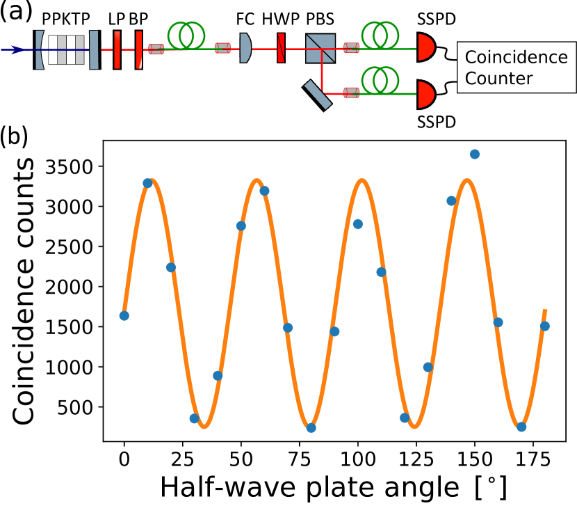
Figure 5: (a) HOM setup to determine the indistinguishability. The SPDC photons are collected by a polarization maintaining single mode fiber and sent through a Fabry-Pérot filter cavity (FC) with a free spectral range of 28 GHz and a linewidth of 850 MHz. The filter cavity is temperature controlled and tuned to the central cavity resonance, where signal and idler are indistinguishable in frequency. The HOM effect can be observed by rotating the HWP and measuring the coincidences after the PBS. The pair is distinguishable when the photons have horizontal and vertical polarization, respectively, and split deterministically at the PBS, leading to the maximum coincidence rate. When the photons have diagonal and anti-diagonal polarization, they are indistinguishable in polarization at the PBS and photon bunching occurs. This leads to a reduction of the coincidence rate to a minimum. (b) The coincidences (blue dots) are measured for several HWP positions. The fluctuation of the coincidences clearly shows the variation of the bunching behavior. A fit (solid orange line) reveals a HOM visibility of 86 $\pm$ 5%.

Appendix G Beam Calibration

We use a strongly attenuated laser beam to characterize the interferometer paths. It is important that the calibration beam contains mainly single photons. To purify the attenuated laser in post processing, all detection events are discarded when more than one photon was detected within 400 ns. The count rates are detected while the phase in each arm is varied by the piezos. We normalize the detected raw counts $D$ with the sum of the counts in the corresponding interferometer arm

$$N_{i}=\frac{D_{i}}{D_{i}+D_{j}},$$ (52)

where $N_{i}$ is the normalized count rate, the index $i$ belongs to the considered detection path and the index $j$ to the corresponding other detection path of the same interferometer arm. This normalization ensures a maximum value of 1 and renders the result independent of the integration time or slow drifts of the laser intensity. Fig. (6-a) shows the normalized count rates for arm 1 for roughly 20 minutes. The discontinuous jumps in the count rates indicate when the piezo is moved back to its starting position without additional data being acquired. It can be seen clearly that the counts are changing deterministically with the piezo voltage. The minimum of $\braket{N_{1}}$ is reached when $\braket{N_{2}}$ is at its maximum which shows that there is destructive interference at detector 1 when there is constructive interference at detector 2. For optimal interference, the counts would range from zero to one. However, background and imperfect mode overlap at the BS reduces this range. To describe this reduction, we determine the average count rate $\bar{c}_{i}$ and the interference visibility $v_{i}$ for each detection path with the detected counts and Eq. (24). This was done every 20 minutes of the measurement to reduce the influence of slow drifts or power fluctuations of the laser. Even though we apply a linear voltage change at the piezos, the piezo response is not truly linear. This effect was stronger for the piezo in interferometer arm 1. Therefore, we used an average of the ten largest and the ten smallest count rates respectively to calculate the parameters $\bar{c}_{i}$ and $v_{i}$, instead of using a sinusoidal fit.

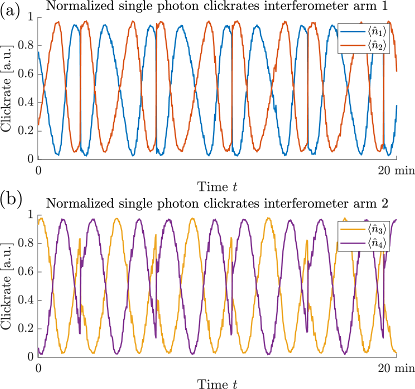
Figure 6: Normalized detected counts for several measurement steps while the piezo voltages are changed after each step. (a) $\braket{N_{1}}$ (blue line) is at its minimum when $\braket{N_{2}}$ (red line) reached its maximum and vice versa. This clearly shows the interference of the interferometer arm 1. The discontinuous jumps indicate the returning of the piezos to their starting position without data acquisition. At the beginning of the measurement, the piezo is not at its starting position, since the piezo voltage is controlled independently from the data acquisition. (b) same for interferometer arm 2 with $\braket{N_{3}}$ (yellow line) and $\braket{N_{4}}$ (purple line).

The bottom of Fig. (3-a) (main text) shows the retrieved reference phases $\phi_{1}$ and $\phi_{2}$ from a calibration measurement of 20 minutes using Eq. (25). It can be seen clearly that $\phi_{1}$ is first constantly decreasing until it reaches zero. Afterwards, $\phi_{1}$ increases linearly up to its maximum $\pi$, after which it decreases again. $\phi_{2}$ behaves similar but with an offset compared to $\phi_{1}$. This phase difference between $\phi_{1}$ and $\phi_{2}$ is caused by the different relative optical path lengths in the two interferometer arms.

Appendix H Filter threshold

The phase retrieval of Eq. (25) uses an $\arccos$, which exhibits a steep slope at the beginning and the end of its domain. Therefore, small fluctuations during the calibration measurement have a greater influence on the retrieved phase, when the retrieved phase is close to 0 or $\pi$. Hence, we filter out data points when the phases $\phi_{1}$ and $\phi_{2}$ are in the range of $0+t$ or $\pi-t$, where $t$ is the filter threshold. The optimal threshold $t$ of such filtering removes the margins with higher uncertainty and simultaneously keeps as much data points as possible to obtain an over-all lower fit uncertainty. Fig. (7) shows the calculated exchange phase $\phi_{x}$ for different thresholds $t$. The lowest uncertainty is reached for a filter threshold of $t=0.25$ rad, with an exchange phase of $\phi_{x}=(-0.04\pm 0.07)$ rad. The uncertainty is increasing for $t>0.25$ rad, since the number of data points for calculating $\phi_{x}$ decreases rapidly. However, all calculated exchange phases $\phi_{x}$ agree within the limits of errors with the bosonic exchange phase of zero.

Figure 7: Calculated exchange phase $\phi_{x}$ for different filter thresholds $t$. The slope of the $\arccos$ diverges for the retrieved reference phases $\phi_{1(2)}$ close to 0 and $\pi$, leading to higher uncertainties for small fluctuations during the calibration measurement. Filtering out these data points can reduce the fit error of the exchange phase $\phi_{x}$, which is decreasing until $t=0.25$ rad. The uncertainty is increasing again for $t>0.25$ rad since too many data points are filtered out. The exchange phase $\phi_{x}=(-0.04\pm 0.07)$ rad at $t=0.25$ rad has the lowest uncertainty and is the main finding of this work.

References

(1)
J. M. Leinaas and J. Myrheim, “On the theory of identical particles,” Il
Nuovo Cimento B (1971-1996), vol. 37, pp. 1–23, Jan 1977.
(2)
W. Pauli, “Über den Zusammenhang des Abschlusses der Elektronengruppen
im Atom mit der Komplexstruktur der Spektren,” Zeitschrift fur
Physik, vol. 31, pp. 765–783, Feb. 1925.
(3)
K. B. Davis, M. O. Mewes, M. R. Andrews, N. J. van Druten, D. S. Durfee, D. M.
Kurn, and W. Ketterle, “Bose-einstein condensation in a gas of sodium
atoms,” Phys. Rev. Lett., vol. 75, pp. 3969–3973, Nov 1995.
(4)
A. M. L. Messiah and O. W. Greenberg, “Symmetrization postulate and its
experimental foundation,” Phys. Rev., vol. 136, pp. B248–B267, Oct
1964.
(5)
J. J. Sakurai and J. Napolitano, Modern Quantum Mechanics.
Cambridge University Press, 2 ed., 2017.
(6)
I. Walmsley, “Quantum interference beyond the fringe,” Science,
vol. 358, no. 6366, pp. 1001–1002, 2017.
(7)
C. K. Hong, Z. Y. Ou, and L. Mandel, “Measurement of subpicosecond time
intervals between two photons by interference,” Phys. Rev. Lett.,
vol. 59, pp. 2044–2046, Nov 1987.
(8)
E. Bocquillon, V. Freulon, J.-M. Berroir, P. Degiovanni, B. Plaçais,
A. Cavanna, Y. Jin, and G. Fève, “Coherence and indistinguishability of
single electrons emitted by independent sources,” Science, vol. 339,
no. 6123, pp. 1054–1057, 2013.
(9)
A. Perez-Leija, D. Guzmán-Silva, R. d. J. León-Montiel, M. Gräfe,
M. Heinrich, H. Moya-Cessa, K. Busch, and A. Szameit, “Endurance of quantum
coherence due to particle indistinguishability in noisy quantum networks,”
npj Quantum Information, vol. 4, no. 1, p. 45, 2018.
(10)
F. Nosrati, A. Castellini, G. Compagno, and R. Lo Franco, “Robust entanglement
preparation against noise by controlling spatial indistinguishability,” npj Quantum Information, vol. 6, no. 1, p. 39, 2020.
(11)
A. Castellini, R. Lo Franco, L. Lami, A. Winter, G. Adesso, and G. Compagno,
“Indistinguishability-enabled coherence for quantum metrology,” Phys.
Rev. A, vol. 100, p. 012308, Jul 2019.
(12)
R. C. Hilborn and C. L. Yuca, “Spectroscopic test of the symmetrization
postulate for spin-0 nuclei,” Phys. Rev. Lett., vol. 76,
pp. 2844–2847, Apr 1996.
(13)
G. Modugno, M. Inguscio, and G. M. Tino, “Search for small violations of the
symmetrization postulate for spin-0 particles,” Phys. Rev. Lett.,
vol. 81, pp. 4790–4793, Nov 1998.
(14)
D. English, V. V. Yashchuk, and D. Budker, “Spectroscopic test of
bose-einstein statistics for photons,” Phys. Rev. Lett., vol. 104,
p. 253604, Jun 2010.
(15)
S. Ospelkaus, K.-K. Ni, D. Wang, M. H. G. de Miranda, B. Neyenhuis,
G. Quéméner, P. S. Julienne, J. L. Bohn, D. S. Jin, and J. Ye,
“Quantum-state controlled chemical reactions of ultracold potassium-rubidium
molecules,” Science, vol. 327, no. 5967, pp. 853–857, 2010.
(16)
K. Levin, A. L. Fetter, and D. M. Stamper-Kurn, Ultracold Bosonic and
Fermionic Gases.
Cambridge University Press, 1 ed., 2012.
(17)
E. Ramberg and G. A. Snow, “Experimental limit on a small violation of the
pauli principle,” Phys. Lett. B, vol. 238, p. 438, Nov. 1990.
(18)
M. de Angelis, G. Gagliardi, L. Gianfrani, and G. M. Tino, “Test of the
symmetrization postulate for spin-0 particles,” Phys. Rev. Lett.,
vol. 76, pp. 2840–2843, Apr 1996.
(19)
D. DeMille, D. Budker, N. Derr, and E. Deveney, “Search for
exchange-antisymmetric two-photon states,” Phys. Rev. Lett., vol. 83,
pp. 3978–3981, Nov 1999.
(20)
R. Mirman, “Experimental meaning of the concept of identical particles,” Il Nuovo Cimento B (1971-1996), vol. 18, no. 1, pp. 110–122, 1973.
(21)
P. Landshoff and H. P. Stapp, “Parastatistics and a unified theory of
identical particles,” Ann. of Phys., vol. 45, p. 72, Jan 1967.
(22)
A. Peres, Quantum Theory: Concepts and Methods.
Springer, Dordrecht, 1 ed., 2002.
(23)
Y. Aharonov and J. Anandan, “Phase change during a cyclic quantum evolution,”
Phys. Rev. Lett., vol. 58, pp. 1593–1596, Apr 1987.
(24)
K. Wang, S. Weimann, S. Nolte, A. Perez-Leija, and A. Szameit, “Measuring the
aharonov–anandan phase in multiport photonic systems,” Opt. Lett.,
vol. 41, pp. 1889–1892, Apr 2016.
(25)
C. F. Roos, A. Alberti, D. Meschede, P. Hauke, and H. Häffner, “Revealing
quantum statistics with a pair of distant atoms,” Phys. Rev. Lett.,
vol. 119, p. 160401, Oct 2017.
(26)
B. Altschul, “Testing photons’ bose-einstein statistics with compton
scattering,” Phys. Rev. D, vol. 82, p. 101703, Nov 2010.
(27)
S. J. van Enk, “Exchanging identical particles and topological quantum
computing,” 2018.
(28)
“See supporting material,”
(29)
A. Messiah, Quantum Mechanics.
Dover, 1 ed., 1999.
(30)
U. Sinha, C. Couteau, T. Jennewein, R. Laflamme, and G. Weihs, “Ruling out
multi-order interference in quantum mechanics,” Science, vol. 329,
no. 5990, pp. 418–421, 2010.
(31)
J. Sperling, W. Vogel, and G. S. Agarwal, “True photocounting statistics of
multiple on-off detectors,” Phys. Rev. A, vol. 85, p. 023820, Feb
2012.
(32)
O. S. Magaña-Loaiza, R. d. J. León-Montiel, A. Perez-Leija, A. B.
U’Ren, C. You, K. Busch, A. E. Lita, S. W. Nam, R. P. Mirin, and T. Gerrits,
“Multiphoton quantum-state engineering using conditional measurements,”
npj Quantum Information, vol. 5, no. 1, p. 80, 2019.
(33)
R. Heilmann, J. Sperling, A. Perez-Leija, M. Gräfe, M. Heinrich, S. Nolte,
W. Vogel, and A. Szameit, “Harnessing click detectors for the genuine
characterization of light states,” Scientific Reports, vol. 6, no. 1,
p. 19489, 2016.
(34)
R. J. Glauber, “Coherent and incoherent states of the radiation field,” Phys. Rev., vol. 131, pp. 2766–2788, Sep 1963.
(35)
E. C. G. Sudarshan, “Equivalence of semiclassical and quantum mechanical
descriptions of statistical light beams,” Phys. Rev. Lett., vol. 10,
pp. 277–279, Apr 1963.
(36)
J. Sperling, W. Vogel, and G. S. Agarwal, “Sub-binomial light,” Phys.
Rev. Lett., vol. 109, p. 093601, Aug 2012.
(37)
C. Gerry and P. Knight, Introductory Quantum Optics.
Cambridge University Press, 2004.