Privug: Using Probabilistic Programming for Quantifying Leakage in Privacy Risk Analysis

Abstract

Disclosure of data analytics results has important scientific and commercial justifications. However, no data shall be disclosed without a diligent investigation of risks for privacy of subjects. Privug is a tool-supported method to explore information leakage properties of data analytics and anonymization programs. In Privug, we reinterpret a program probabilistically, using off-the-shelf tools for Bayesian inference to perform information-theoretic analysis of the information flow. For privacy researchers, Privug provides a fast, lightweight way to experiment with privacy protection measures and mechanisms. We show that Privug is accurate, scalable, and applicable to a range of leakage analysis scenarios.

1 Introduction

However high the value of data becomes, we cannot ignore the risks that data disclosure presents to personal privacy. Consequently, general privacy protection methods like differential privacy [18], comprehensibility and communication of privacy issues [32], industrial processes for data management [22], and debugging and analyzing privacy risk problems in program code [11, 12, 9] have become intensive areas of research. This paper falls into this last group; we present tools for data scientists who create data analysis programs and would like to disclose the results of the computation. Our primary goal is to create a method that supports a privacy debugging process, i.e. assessing effectiveness of such algorithms, and indeed of any calculations on the data, for concrete programs and datasets, in the style of debuggers. We want to help identifying and explaining the leakage risks, as the first step towards eliminating them.

As an example, consider the following Scala program that, given a list of names and ages, computes the mean age of the persons in a map-reduce style:

⬇ @ifdisplaystyle 1def agg (records: List[(String,Double)]): Double = 2 records.map { (n, a) => (a, 1) } 3 .reduce { (x, y) => (x._1 + y._1, x._2 + y._2) } 4 .map { (sum, count) => sum / count }

Let the age of each individual be the sensitive secret in this example. One attack could be that underage individuals can be identified. An analyst would like to ask: How much of sensitive information leaks when the mean is disclosed? In what situations is this leak not ignorable? What kind of attackers may discover the secret by observing the mean?

Privug is an analysis method for privacy risks in data processing. A data analyst using Privug models an attacker’s knowledge about the secret as a probability distribution. Privug re-interprets the program as an information transformer that operates on distributions instead of concrete inputs. The analyst analyzes the attacker’s confidence about the secret, using a combination of probability queries, standard information-theoretic measures, and visualizations. She explores and assesses the information leakage to the result of the program by varying attacker knowledge, the queries and the leakage measures. For our example, the analyst may learn that the leakage is ignorable if the subjects are drawn from general population, but if the attacker knows that they come from a homogeneous group, she could, for example, conclude that a specific individual is under age.

Since Privug is based on probabilistic reasoning, it can be facilitated by probabilistic programming, a lively field in data science, with many tools available. Privug is not tied to any particular probabilistic programming framework. In this paper, we implement queries, measures, and visualization in Figaro [34] and PyMC3 [39]. For programs seen as functions, a probabilistic programming framework can automatically build a Bayesian model which represents the information transform. This transform supplemented by a model of attacker can be used to explore re-identification risks [14].

Privug offers three distinct advantages over state of the art tools for privacy risk analysis: (i) It focuses on the analysis of programs not data, which means that a what-if analysis can be performed before data is available, or without authorizing access to a sensitive database. (ii) It is largely automatable using off-the-shelf systematic Monte-Carlo inference tools already used by data analysts, but which have not been used for this purpose before. (iii) Privugis easy to extend with new estimators of leakage thus serves as a good test-bed for privacy mechanism research. To the best of our knowledge, Privug as a method and probabilistic programming as a platform are the only basis that can offer such versatility at this point. Our contributions include:

1. A widely applicable and extensible method, Privug, to analyze privacy risks. The first such method based on probabilistic programming frameworks.

2. An implementation of Privug in Figaro and PyMC3, the first versatile tool supporting such a wide range of measures over continuous and discrete inputs and outputs.

3. An empirical evaluation of the accuracy, scalability, and applicability of Privug for analyzing systems of different size and complexity, showing that probabilistic programming is an excellent base for implementing leakage analysis tools.

We evaluate applicability, accuracy, and scalability of Privug, using well known privacy mechanisms (differential privacy, $k$-anonymity, naive anonymization) and synthetic cases that can be scaled up for higher dimensionality and using. Our experiments demonstrate Privug’s versatility to realize many analysis scenarios, and its interoperability with existing tools (by integrating external estimators). The source code and experiment data is available at https://bitbucket.org/itu-square/privug-experiments. The repository contains additional experiments showing the use of Privug in a realistic case study: an experiment using the differential privacy library OpenDP (https://opendp.org/).

name	zip	birthday	sex	diag.
Alice	2300	15.06.1954	F	ill
Bob	2305	15.06.1954	M	healthy
Carol	2300	09.10.1925	F	healthy
Dave	2310	01.01.2000	M	ill

${\xrightarrow{\text{\leavevmode\lstinline{{\lst@@@set@language\lst@@@set@numbers\lst@@@set@frame\lst@@@set@rulecolor\lst@@@set@numbers\normalsize{\@listingGroup{ltx_lst_keywords5}{\color[rgb]{0.59,0.44,0.84}ano}}}}}}}$ zip birthday sex diag. 2300 15.06.1954 F ill 2305 15.06.1954 M healthy 2300 09.10.1925 F healthy 2310 01.01.2000 M ill

zip	birthday	sex	diag.
2300	15.06.1954	F	ill
2305	15.06.1954	M	healthy
2300	09.10.1925	F	healthy
2310	01.01.2000	M	ill

$\oplus$ name zip birthday sex Mark 2450 30.09.1977 M Rose 2870 24.12.1985 F Alice 2300 15.06.1954 F Dave 2310 01.01.2000 M $\rightsquigarrow$ Alice is ill

Figure 1: Privacy violation: The data is anonymized (@ifdisplaystyleano), then the diagnosis of Alice is recovered by an attacker who links the result with another data set ($\oplus$).

name	age
Alice	42
Bob	25
Carol	25
Dave	25

${\xrightarrow{\text{\leavevmode\lstinline{{\lst@@@set@language\lst@@@set@numbers\lst@@@set@frame\lst@@@set@rulecolor\lst@@@set@numbers\normalsize{\@listingGroup{ltx_lst_keywords5}{\color[rgb]{0.59,0.44,0.84}agg}}}}}}\,}$ 29.25 $\oplus$     name age Alice $\mathcal{N}$(40,3) Bob $\mathcal{N}$(23,10) Carol $\mathcal{N}$(23,10) Dave $\mathcal{N}$(23,10) $\rightsquigarrow$ Alice’s age is
$\mathcal{N}$(41,2.5)

Figure 2: Privacy violation: The program computes a mean of ages, the mean is released, but an attacker with prior knowledge can reduce the uncertainty regarding Alice’s age.

name	age
Alice	42
Bob	25
Carol	25
Dave	25

${\xrightarrow{\text{\leavevmode\lstinline{{\lst@@@set@language\lst@@@set@numbers\lst@@@set@frame\lst@@@set@rulecolor\lst@@@set@numbers\normalsize{\@listingGroup{ltx_lst_keywords5}{\color[rgb]{0.59,0.44,0.84}agg}}}}}}\,}$ 29.25 $\oplus$     name age Alice $\mathcal{N}$(40,3) Bob $\mathcal{N}$(23,10) Carol $\mathcal{N}$(23,10) Dave $\mathcal{N}$(23,10) $\rightsquigarrow$ Alice’s age is
$\mathcal{N}$(41,2.5)

Figure 3: Privacy violation: The program computes a mean of ages, the mean is released, but an attacker with prior knowledge can reduce the uncertainty regarding Alice’s age.

fig:example2

2 Overview

name	age
Alice	42
Bob	25
Carol	25
Dave	25

${\xrightarrow{\text{\leavevmode\lstinline{{\lst@@@set@language\lst@@@set@numbers\lst@@@set@frame\lst@@@set@rulecolor\lst@@@set@numbers\normalsize{\@listingGroup{ltx_lst_keywords5}{\color[rgb]{0.59,0.44,0.84}agg}}}}}}\,}$ 29.25 $\oplus$     name age Alice $\mathcal{N}$(40,3) Bob $\mathcal{N}$(23,10) Carol $\mathcal{N}$(23,10) Dave $\mathcal{N}$(23,10) $\rightsquigarrow$ Alice’s age is
$\mathcal{N}$(41,2.5)

Figure 4: Privacy violation: The program computes a mean of ages, the mean is released, but an attacker with prior knowledge can reduce the uncertainty regarding Alice’s age.

fig:example2

3 Overview

sec:overview We consider data disclosure programs seen as functions that transform an input dataset to an output. The output is then disclosed to a third party, called an attacker. The aggregation example agg from the introduction translates a database with two columns: name (String) and age (Double) to a number representing mean age which is then published. The second running example, ano, anonymizes medical records in a dataset. The input data has five columns: name, zip code, birthday, sex, and diagnosis. The program simply drops the name column, before the data is released to an attacker:

4 Privug

We present each step of the Privug method in detail. We model disclosure problems probabilistically and express models directly in a probabilistic programming language to enable automatic analysis. Let $D(X)$ denote a distribution over a set $X$. We write $x\sim D(X)$ to denote that random variable $x$ is distributed according to $D(X)$; thus $x\sim\mathcal{U}(0,10)$ means that $x$ is uniformly distributed from $0$ to $10$. In a programming language, this corresponds to x = Uniform(0,10). We also use composition operators of the language to define $y$ in terms of $x$, define a distribution over datasets, and so on.

Step 1: Attacker Knowledge (Prior).

We model the prior knowledge of an attacker as a probability distribution over the possible input values of the program. In the agg program the input ranges over an array of pairs (name,age). Therefore, attacker prior knowledge is defined as a distribution over lists of pairs, ${D(\text{\leavevmode\lstinline{{\lst@@@set@language\lst@@@set@numbers\lst@@@set@frame\lst@@@set@rulecolor\lst@@@set@numbers\normalsize{\@listingGroup{ltx_lst_keywords4}{\color[rgb]{0.72,0.53,0.04}List}}[({\@listingGroup{ltx_lst_keywords3}{\color[rgb]{0.85,0.65,0.13}String}},{\@listingGroup{ltx_lst_keywords3}{\color[rgb]{0.85,0.65,0.13}Double}})]}}}})$. Consider the following two examples of attackers:

1. The knows-a-lot attacker knows that the input dataset contains exactly four rows and that the age of all individuals, except Alice, is $55.2$. This is modeled by distributions $\mathcal{C}$(4) for the size and $\mathcal{C}$(55.2) for the age column.

2. The knows-just-a-bit attacker knows that the input has approximately hundred entries ($|\textit{records}|\sim\mathcal{B}(300,\nicefrac{{1}}{{3}})$, a binomial distribution), and that the average age of an individual in the list is 55 (distributed with $\mathcal{N}(55.2,3.5)$).

Both attackers know that Alice’s record is in the dataset, and that no other record in the dataset has that name. They do not know anything about Alice’s age upfront: all ages from 0 to 100 are equally likely, a uniform distribution $\mathcal{U}(0,100)$. Implementations of ${\mathrm{k}_{\mathrm{al}}}$ and ${\mathrm{k}_{\mathrm{ab}}}$ are shown below, the differences highlighted in bold. Here, Element[T] denotes a distribution over T, and FixedSizeArrayElement[T] denotes a distribution over fixed-but-unknown-size arrays of Ts. When sampled, ${\mathrm{k}_{\mathrm{ab}}}$ yields an array of random size, containing (String,Double) pairs. The first pair represents Alice.

⬇

@ifdisplaystyle

1def prior_kal: FixedSizeArrayElement[(String,Double)] =

2 VariableSizeArray (Constant (4), i => for

3 n <- if i==0 then Constant ("Alice") else Uniform (names: _*)

4 a <- if i==0 then Uniform (0,100) else Constant (55.2)

5 yield (n, a))

7def prior_kab: FixedSizeArrayElement[(String,Double)] =

8 VariableSizeArray (Binomial (300, 0.3), i => for

9 n <- if i==0 then Constant ("Alice") else Uniform (names: _*)

10 a <- if i==0 then Uniform (0,100) else Normal (55.2,3.5)

11 yield (n, a))

Step 2: Attacker Prediction (Program).

We obtain the attacker’s prediction of the output of running a program by transforming—i.e.  lifting—the program to operate on distributions instead of concrete datasets, and applying it to the attacker model. Let $\mathcal{D}{}(X)$ denote the set of distributions on set $X$. Since distributions form a monad [35], several useful functions are well defined on distributions, including $\mathbf{lift}\,$ that, here, has type

$${\mathbf{lift}\,{}}:\big{(}A\to B\big{)}\to\big{(}\mathcal{D}{}(A)\to\mathcal{D}{}(B)\big{)}.$$

A function from $A$ to $B$ becomes a function from distributions over $A$ to distributions over $B$. Recall that the type of agg is List[(String, Double)] $\to$ Double. The lifting of agg has type: ${\mathcal{D}{}(\text{\leavevmode\lstinline{{\lst@@@set@language\lst@@@set@numbers\lst@@@set@frame\lst@@@set@rulecolor\lst@@@set@numbers\normalsize{\@listingGroup{ltx_lst_keywords4}{\color[rgb]{0.72,0.53,0.04}List}}[({\@listingGroup{ltx_lst_keywords3}{\color[rgb]{0.85,0.65,0.13}String}},{\@listingGroup{ltx_lst_space}{ }}{\@listingGroup{ltx_lst_keywords3}{\color[rgb]{0.85,0.65,0.13}Double}})]}}}})$ $\to$ ${\mathcal{D}{}(\text{\leavevmode\lstinline{{\lst@@@set@language\lst@@@set@numbers\lst@@@set@frame\lst@@@set@rulecolor\lst@@@set@numbers\normalsize{\@listingGroup{ltx_lst_keywords3}{\color[rgb]{0.85,0.65,0.13}Double}}}}}})$. In Figaro:

⬇

@ifdisplaystyle

1def agg_p (records: FixedSizeArrayElement[(String,Double)]): Element[Double] =

2 records.map { (n, a) => (a, 1) }

3 .reduce { (x, y) => (x._1 + y._1, x._2 + y._2) }

4 .map { (sum, count) => sum / count }

Note that only types change; $\mathcal{D}$ is Element in Figaro, and FixedSizeArrayElement[T] is an efficient implementation of ${\mathcal{D}{}(\text{\leavevmode\lstinline{{\lst@@@set@language\lst@@@set@numbers\lst@@@set@frame\lst@@@set@rulecolor\lst@@@set@numbers\normalsize{\@listingGroup{ltx_lst_keywords4}{\color[rgb]{0.72,0.53,0.04}List}}[{\@listingGroup{ltx_lst_identifier}{T}}]}}}})$. For a distribution over input datasets, agg_p yields a distribution over average ages (Double). Running agg_p on a prior modeling the attacker’s knowledge yields the attacker’s prediction of the average age. Formally, the distribution of the output (the attacker prediction) is defined as $\mathit{P}(o)=\int_{x}\mathit{P}(o|x)\mathit{P}(x)dx$. 0.A describes the semantic details of computing $\mathit{P}(o)$.

Step 3: Attacker Observation.

We use observations to condition the attacker’s prediction of the output. Since the prediction depends on the prior, conditioning it conditions the prior, and updates the attacker’s knowledge about the input. We write $\mathit{P}(x\,|\,E)$ to denote the conditional distribution of $x$ given evidence $E$. Let $x\sim D(X)$, the evidence $E$ is a predicate over $X$. For instance, we write $\mathit{P}(x\,|\,4<x<8)$ to denote the conditional distribution where only the outcomes $x$ in the interval $(4;8)$ are possible. We use conditions to model attacker observations of the output. For our aggregation example, to assert that the attacker observes 55.3, we define the predicate $E$ as (x : Double) => (55.295<=x && x<55.305) as evidence on the prediction. The observation is typically known as likelihood function [26], and it is modeled as a distribution (denoted as $\mathit{P}(E|x)$) assigning high probability to the values satisfying $E$. For instance, for the observation above we define $\mathit{P}(E|x)$ equals $1/0.005$ for $55.295\leq x\leq 55.305$ and $0$ otherwise. In Scala, the predicate $E$ is written as an anonymous function stating that the output is within $0.005$ from $55.3$. We cannot assert that the output is exactly $55.3$, since the output space is continuous; each individual outcome occurs with probability zero. In Figaro, we set $E$ on prediction o with o.setCondition($E$).

Step 4: Attacker Posterior.

We use Bayesian inference to compute the updated attacker’s knowledge upon the observation. We put together the elements of our model using the Bayes rule as follows:

$$\underbrace{\mathit{P}(x,o\,|\,E)}_{\mathit{posterior}}={\underbrace{\mathit{P}(E\,|\,x,o)}_{\mathit{observation}}\cdot\overbrace{P(o|x)\cdot\underbrace{\mathit{P}(x)}_{\mathit{prior}}}^{\mathit{prediction}}\cdot\mathit{P}(E)^{-1}}\vspace*{-0mm}$$ (1)

Our goal is to use the attacker prior $\mathit{P}(x)$ (step 1), attacker prediction $\mathit{P}(x,o)=\mathit{P}(o|x)\mathit{P}(x)$ (step 2), and observation $\mathit{P}(E|x,o)$ (step 3) to compute the posterior knowledge $\mathit{P}(x,o|E)$. Note that the equation above is expressed in terms of the joint distribution of the random variables for input $x$ and output $o$. The marginal distributions can be obtained by integrating out the corresponding variables. We use Markov Chain Monte Carlo (MCMC) methods [37] to estimate the posterior distribution by generating samples from a probabilistic program. MCMC algorithms are simulation methods that efficiently generate samples from the high density intervals of the target distribution, in our case $P(x,o|E)$. We refer the interested readers to Robert and Casella [37] for details. We consider only terminating programs; as no samples can be generated from non-terminating programs using these methods. We remark that MCMC methods do not require computing or specifying the normalization factor $\mathit{P}(E)^{-1}$. Their convergence conditions are well-known [21], but the number of samples determines their accuracy. In Sect. 5, we evaluate the accuracy and efficiency of several MCMC methods for this application. In Figaro, we use the MCMC algorithm importance sampling [34]. Let $a$ and $o$ denote Alice’s age and the outcome in the aggregation example. If we define the evidence $E=\text{``}o\approx 55.3\text{''}$ on the prediction as above, Importance(10000, a) produces $10000$ samples that estimate the distribution $\mathit{P}(a\,|\,o\approx 55.3)$.

Step 5: Leakage (Posterior Analysis).

		${\mathrm{k}_{\mathrm{al}}}$	${\mathrm{k}_{\mathrm{ab}}}$				${\mathrm{k}_{\mathrm{al}}}$	${\mathrm{k}_{\mathrm{ab}}}$
Expectation	$\mathrm{E}[a|o\approx 55.3]$	$55.60$	$64.000$		Standard deviation	$\sigma[a|o\approx 55.3]$	$0.01$	$14.00$
Probability query	$\mathit{P}(a|o\approx 55.3)$	$0.00$	$0.004$		Shannon Entropy	$\mathrm{H}(a|o\approx 55.3)$	$-3.08$	$5.83$
KL-divergence	$\mathrm{D}_{\mathrm{KL}}(a|o\approx 55.3\mid\mid a)$	$5.64$	$0.770$		Mutual Information	$\mathrm{I}(a;o)$	$9.37$	$0.60$

Table 1: Posterior analysis summary. Results of each measure for the two attackers.

We analyze the posterior distribution to investigate what the attacker learns. Table 1 shows an overview of analyses for the agg example. Using multiple measures gives a multi-perspective analysis for complex problems. To query the probability $\mathit{P}(x\!\mid\!\varphi)$ of a random variable $x$ satisfying a predicate $\varphi$, in Figaro we write alg.probability($x$,$\varphi$) where alg is the inference algorithm. Other available queries estimate the histogram of the attacker’s posterior, its expectation, and variance. The probability query allows to estimate whether an attacker learns a fact, effectively encoding a knowledge-based security policy check (Sect. 6). The strengths of an attack checking if Alice is underage in the agg example is captured by the query: $\mathit{P}\left(a\!<\!18\mid o\!\approx\!55.3\right)$. The prior probability of $a\!<\!18$ is $0.17$. It reduces to $0.004$ for ${\mathrm{k}_{\mathrm{ab}}}$ and to 0 for ${\mathrm{k}_{\mathrm{al}}}$ in the posterior. Both attackers can conclude that Alice is an adult. To visualize information gain, we plot the kernel density estimates [40]. 6 plots the age of Alice in the prior $P(a)$ and the posterior $\mathit{P}(a\mid o\!\approx\!55.3)$ for ${\mathrm{k}_{\mathrm{al}}}$. 6 shows the same for o = agg_p(prior_kab). The plots confirm that ${\mathrm{k}_{\mathrm{al}}}$ can make stronger conclusions than ${\mathrm{k}_{\mathrm{ab}}}$; the posterior of the former is taller and narrower than the one of the latter; note the y-axis scale. The uniform prior has expected value $\mathrm{E}[a]\!\approx\!50$ and standard deviation $\sigma_{a}\!\approx\!29$. As listed in Tbl. 1, the posterior expectation increases to 55.60 for ${\mathrm{k}_{\mathrm{al}}}$ with standard deviation 0.01: ${\mathrm{k}_{\mathrm{al}}}$ effectively learns $a$ from the output. For ${\mathrm{k}_{\mathrm{ab}}}$ the posterior has larger standard deviation (14), so ${\mathrm{k}_{\mathrm{ab}}}$’s uncertainty about the age of Alice is greatly reduced, yet remains high. Moving beyond measuring and visualizing probability, we quantify attacker’s learning using quantitative information flow measures: entropy, KL-divergence, mutual information, and Bayes risk. These and other measures are added to Privug as libraries, which estimate the corresponding measure using the samples of the MCMC algorithm of Step 4. Shannon’s entropy quantifies the uncertainty about the value of a random variable (e.g., [30, 24]). A decrease in entropy from prior to posterior signifies an increase in knowledge. Entropy (in bits) is defined as $\mathrm{H}(x)=\sum_{x\in X}\mathit{P}(x)\log_{2}\mathit{P}(x)$ for discrete random variables. Since Privug works with an inferred distribution, we estimate the entropy using the classic algorithm [1], which is known to be accurate and easy to implement. In the agg example, the entropy of $a$ in the prior is $\mathrm{H}(a)=6.67$ bits. At the same time, the conditional entropy of $a$ in the posterior for ${\mathrm{k}_{\mathrm{ab}}}$ is $\mathrm{H}(a\,|\,o\approx 55.3)=5.84$ bits. The attacker gained $0.83$ bits of information about the age of Alice. For ${\mathrm{k}_{\mathrm{al}}}$, the posterior entropy is $\mathrm{H}(a\,|\,o\approx 55.3)=-3.08$. Here the difference is $9.75$ bits, twelve times more than what ${\mathrm{k}_{\mathrm{al}}}$ learned. (The entropy of a continuous variable (replace $\sum$ with $\int$ above), differential entropy, can be negative [1].) Clearly, ${\mathrm{k}_{\mathrm{al}}}$ is an example of an attacker able to amplify the disclosed information thanks to its additional pre-existing knowledge—a situation often referred to as a linking attack. The ability of ${\mathrm{k}_{\mathrm{ab}}}$ in this respect is much weaker. Privug allows experimenting with the attacker space in this way, to let the data controller understand what attacks are successful, and then assess whether they are of concern. Relative entropy [28] or KL-divergence measures how much two distributions differ. In Bayesian inference, the KL-divergence of a posterior $P(x)$ and a prior $Q(x)$, defined as $\mathrm{D}_{\mathrm{KL}}(P\mid\mid Q)=\sum P(x)\log_{2}(P(x)/Q(x))$, expresses the amount of “information lost when $Q$ is used to approximate $P$” [6, page 51]. Thus, KL-divergence is a measure of information gained by revising one’s knowledge of the prior to the posterior. As with entropy, since we are working with an inferred distribution, we can estimate KL-divergence from samples. We use the algorithm by Wang et al.  [43]. For the aggregation example, the KL-divergence between the posterior and prior of $a$ is a measure of the amount of information that the attacker gained about Alice’s age by observing the output of the program. For ${\mathrm{k}_{\mathrm{ab}}}$, $\mathrm{D}_{\mathrm{KL}}(a\,|\,o\approx 55.3\mid\mid a)=0.77$. For ${\mathrm{k}_{\mathrm{al}}}$, on the other hand, $\mathrm{D}_{\mathrm{KL}}(a\,|\,o\approx 55.3\mid\mid a)=5.64$. These results indicate that the observation yields an information gain of $0.77$ bits for ${\mathrm{k}_{\mathrm{ab}}}$ and $5.64$ bits for ${\mathrm{k}_{\mathrm{al}}}$. More important is the difference; ${\mathrm{k}_{\mathrm{al}}}$ gains over $7$ times more information than ${\mathrm{k}_{\mathrm{ab}}}$. In 5.0.1 we show how KL-divergence can be used to measure utility when programs add noise to their output. Mutual information between two random variables $x$, $y$, defined as $\mathrm{I}(x;y)=\sum_{y\in Y}\sum_{x\in X}\mathit{P}(x,y)\log_{2}(\mathit{P}(x,y)/\mathit{P}(x)\mathit{P}(y))$, measures the reduction of the uncertainty of $x$ by the knowledge of $y$ [15]. We estimate $\mathrm{I}(i;o)$ where $i$ is a secret input and $o$ a public output (the attacker’s prediction) to quantify how much information $o$ shares with $i$. Mutual information is well studied as a quantitative information flow measure (cf. Sect. 6). A privacy protection mechanism typically aims at minimizing $\mathrm{I}(i;o)$. In Privug, we use the mutual information estimator [25] provided by SKlearn [33] for continuous variables and LeakiEst [11] for discrete variables. In our example, we have $\mathrm{I}(a;o)=9.37$ bits for ${\mathrm{k}_{\mathrm{al}}}$ and $\mathrm{I}(a;o)=0.60$ bits for ${\mathrm{k}_{\mathrm{ab}}}$. This is consistent with our intuition: when the attacker knows everything about the input except for Alice’s age, observing the output greatly reduces their uncertainty. Privug can incorporate estimators of other measures. In Sect. 5 we show that other tools can be incorporated on the example of F-BLEAU [9], to estimate Bayes risk—the expected probability of an attacker guessing a secret ($s$) by observing the output of the program ($o$); formally: $1-\sum_{o\in O}\max_{s\in S}\mathit{P}(o|s)\mathit{P}(s)$ for random variables $s$ and $o$ [2].

This way we determine if specific attackers are capable of learning secrets, and assess whether disclosing the output of the program poses a privacy risk. 5 gives an overview of the steps in the Privug method. Privug’s intended users are data analysts with knowledge in statistics and probabilistic modeling. These users are typically trained in probabilistic programming, an essential part of their toolbox (e.g., [21]). This makes it easy to perform steps 1, 3, and 4. Step 2 typically requires simply updating the datatypes of the input (as in agg and ano). The analyst may, however, need to change the program to ensure differentiability, or replace some operators with their probability counterparts. These are the same techniques that data analysts use to create advanced probabilistic models and analyses. Step 5’s probability queries, visualizations, and distribution statistics such as expected value or variance, are likewise familiar to data analysts. The interpretation of leakage does, however, require privacy-specific expertise (information theory, quantitative information flow). The results and conclusions drawn do depend on the to choice of prior. The prior models what an attacker knows about the input of the program, the secondary knowledge that linked with the observed output can lead to privacy violations. The analysis may report no leakage if priors do not reflect the real information that an attacker has access to. Ideally, priors should be informed from real world data. For instance, if the program takes as input a set of records of US citizens, then it is advisable to inform priors from publicly available sources, e.g., the US census. Alternatively, probabilistic programming frameworks can be used to automatically learn underlying distributions from data with better accuracy than simply using the empirical distributions [21]. For mutual information and multiplicative Bayes capacity (a derived measure from Bayes risk, it has been shown that running the analysis with uniform priors uncovers leakage if it exists, see [13, Theorem 4] and [2, Theorem 7.2]. This result can be used with good effect to detect leakage, but not to estimate its magnitude, which can be estimated using Privug.

Figure 5: Overview of the steps in Privug method.

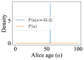
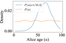
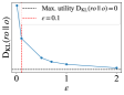
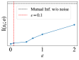
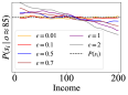
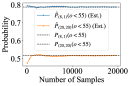
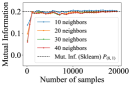
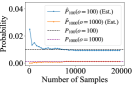
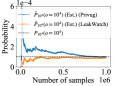
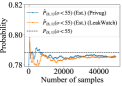
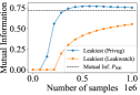
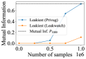
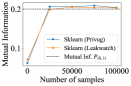
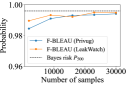
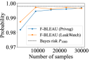
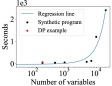
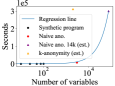
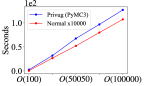
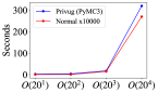
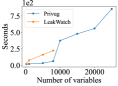
                      (6)                       (6)                       (6)                       (6)                       (6)                       (6)                       (6)                       (6)                       (6)                       (6)                       (6)                       (6) (6)   (6)   (6)   (6)   (6)   (6)   (6)   (6)   (6)   (6)   (6)   (6)   (6)   (6)   (6)   (6)   (6)   (6)   (6)   (6)

Figure 6: Analysis results. Naive Anonymization: Quasi-identifier analysis (6) zip, (6) day, (6) sex, (6) zip+sex, (6) day+sex, (6) zip+day, (6) zip+day+sex. Large datasets: (6) zip+day, (6) zip+day+sex. Sensitive attribute analysis: (6) Chance of learning that governor is ill if 5 share his zip. $k$-anonymity: Number of rows matching governor’s attributes ($k\!=\!2$): (6) sex, (6) any other attribute combination. Aggregate example: Prior and posterior knowledge of age of Alice (distributions): (6) ${\mathrm{k}_{\mathrm{al}}}$, (6) ${\mathrm{k}_{\mathrm{ab}}}$. Differential privacy: (6) Utility, (6) Mutual Information, (6) Probability Queries. Convergence of Privug. (6) Probability query (Continuous), (6) Mutual Information (Continuous), (6) Probability query (Discrete). Comparison w/ LeakWatch: Probability queries (6) Discrete $P_{10000}(o=10000)$, (6) Continuous $P_{(8,1)}(o<55)$. Mutual Information (6) Discrete $P_{500}$ in LeakiEst, (6) Discrete $P_{1000}$ in LeakiEst, (6) Continuous $P_{(8,1)}$ in SKlearn. Bayes Risk: (6) Discrete $P_{500}$ in F-BLEAU, (6) Discrete $P_{1000}$ in F-BLEAU. Scalability of Privug. Inference time: (6) Continuous random variables, (6) Discrete random variables. Time complexity on f(arr,c): (6) Increasing $n\in(10^{2},10^{5})$ for $O(n)$, (6) Increasing $c\in(1,4)$ for $O(20^{c})$. Comparison w/ LeakWatch: (6) $P_{(8,1)}$.

5 Evaluation

5.0.1 RQ1: Can Privug analyze common privacy mechanisms?

We analyze three (modern and traditional) privacy mechanisms in Privug. The purpose is twofold: i) Demonstrate the applicability of Privug, and ii) Serve as templates for data analysts.

Differential Privacy.

Consider a company computing the mean income of employees with agg and releasing the output publicly. To protect the anonymity of employees, they add Laplacian noise to the output; a popular mechanism to enforce differential privacy [18, 19]. We use Privug to explore trade-offs between privacy protection and data utility by varying the values of parameters. We assume a dataset of $200$ incomes. The company have previously released some data on 195 of the 200 incomes, so it is publicly known that they are between $80k and $90k ($\mathcal{U}(80,90)$). There are 5 new employees of which no income information is known ($\mathcal{U}(10,200)$). The program to analyze is an extension of agg that adds Laplacian noise to the output: ${{o\sim\text{\leavevmode\lstinline{{\lst@@@set@language\lst@@@set@numbers\lst@@@set@frame\lst@@@set@rulecolor\lst@@@set@numbers\normalsize{\@listingGroup{ltx_lst_keywords5}{\color[rgb]{0.59,0.44,0.84}agg}}}}}}+\mathcal{L}(0,\Delta\text{\leavevmode\lstinline{{\lst@@@set@language\lst@@@set@numbers\lst@@@set@frame\lst@@@set@rulecolor\lst@@@set@numbers\normalsize{\@listingGroup{ltx_lst_keywords5}{\color[rgb]{0.59,0.44,0.84}agg}}}}}}/\epsilon)$ where ${\Delta\text{\leavevmode\lstinline{{\lst@@@set@language\lst@@@set@numbers\lst@@@set@frame\lst@@@set@rulecolor\lst@@@set@numbers\normalsize{\@listingGroup{ltx_lst_keywords5}{\color[rgb]{0.59,0.44,0.84}agg}}}}}}$ denotes the sensitivity. This is known to preserve $\epsilon$-differential privacy [19, Thm. 3.6]. Sensitivity captures the magnitude by which a single entry can change the output. The program with the mechanism incorporated takes as input the epsilon ($\epsilon$) and a set of records, returning the average income. The implementation in Figaro after lifting is:

⬇

@ifdisplaystyle

1def dp_agg (epsilon: Double, records: FixedSizeArrayElement[(String,Double)]) =

2 val delta = Constant(200.0)/records.length

3 val lambda = Constant(epsilon)/delta

4 val X = continuous.Exponential(lambda)

5 val Y = Flip(0.5) // <-- Bernoulli

6 val laplaceNoise = If(Y, X*Constant(-1.0), X)

7 agg(records) ++ laplaceNoise

Since the maximum income is 200k, the sensitivity (delta) is $\nicefrac{{200}}{{|\mathit{records}|}}$. We construct the Laplace distribution from an exponential and a Bernoulli distributions in lines 2–6 using a standard construction. 7 adds the noise to the result of agg. The Laplacian mechanism includes a notion of accuracy to quantify utility (e.g., [19, Thm 3.8]). Unconventionally, we opt for measuring utility as KL-divergence between the output with noise ($o$) and without ($\mathit{ro}$). The reason is that KL-divergence can be applied to any method based on perturbing the output of the program (demonstrating broad applicability of our currently-supported measures). High KL-divergence indicates low utility as it represents loss of information wrt. the noiseless output. Maximum utility is achieved when KL-divergence equals 0. We observe in 6 an exponential decay of KL-divergence as $\epsilon$ increases, consistent with the intuition that small values of $\epsilon$ result in high noise and reduced utility. The graph suggests that decrements in $\epsilon$ for $\epsilon<0.5$ may impact utility strongly. Now we evaluate how $\epsilon$ influences the flow of information from the income of new employees ($s_{i}$) to the output ($o$). Mutual information is $0$ if one is independent of the other (i.e. no information flow). 6 plots mutual information for different values of $\epsilon$. The dashed line shows the baseline, i.e. mutual information when the output has no added noise. This shows mutual information increases linearly with $\epsilon$. Finally, we use a probability query to evaluate the effect of $\epsilon$ on statistical information that an attacker can learn about the new members in the dataset. Differential privacy does not focus on protecting this type of information—it focuses on protecting the presence of a record in the dataset. Yet it is useful to quantify the effect of the noise on attacker knowledge. Suppose running dp_agg with $\epsilon\!=\!0.5$ yields $85$k as a result. Suppose privacy regulations disallow revealing income data without employee consent. The company would like to determine, whether revealing this result could breach the regulation. In Privug, we analyze the distribution $P(s_{i}\mid o\approx 85)$ to determine this. 6 shows the distributions for different values of $\epsilon$. The dashed line marks the baseline, i.e., the probability distribution before the observation. The blue line corresponds to the run with $\epsilon\!=\!0.5$. Since this line is not parallel with the baseline, there is evidence of an increase in knowledge. The other lines show that any $\epsilon>0.1$ increases the knowledge about the salary of the new employees. Consequently, releasing the average 85k computed using $\epsilon=0.5$ will result in a violation of the regulation. In summary, we have discovered that releasing the average income 85k with $\epsilon>0.1$ reveals information about the salary of new employees. Thus, for $\epsilon=0.5$, the company must seek consent from employees. Mutual information increases linearly with $\epsilon$, and for $\epsilon<0.5$ is notably low. Utility exhibits an exponential decay as $\epsilon$ decreases. This decay is especially pronounced with $\epsilon<1$, showing the impact of the added noise on utility.

Naive Anonymization

We quantify how strongly an attacker can determine the diagnosis of an individual (the governor) by observing the output of ano from LABEL:sec:overview. Though this mechanism has well-known privacy flaws, it is still commonly used. Thus, we illustrate how Privug is used to effectively find these flaws. First, we define the prior. In Figaro:

⬇

@ifdisplaystyle

1def  p : FixedSizeArrayElement[(Name,Zip,Day,Sex,Diag)] = 

2 VariableSizeArray (Constant (1000), i => for

3 n <- if i==0 then Constant (GNAME) else Uniform (names:_*)

4 z <- if i==0 then Constant (GZIP) else Uniform (zips:_*)

5 b <- if i==0 then Constant (GDAY) else Uniform (days:_*)

6 s <- if i==0 then Constant (GSEX) else Uniform (Male,Female)

7 d <- if i==0 then Constant (GILL) else If (Flip (.2), Ill, Healthy)

8 yield (n,z,b,s,d))

Name is an identifier for an individual. For the sake of clarity, we assume that Zip, Day and Sex are non-sensitive attributes, and Diag is sensitive. Name, Zip, Day and Sex are uniformly distributed, and Diag is Ill with probability 0.2. The first row in the dataset is fixed, containing the governor’s record. The prior fixes a dataset size of $1000$ records. The lifted version of ano follows. Note that, compared to ano, only the type changed.

⬇

@ifdisplaystyle

1def ano_p (records : FixedSizeArrayElement[(Name,Zip,Day,Sex,Diag)]) =

2 records.map { (n, z, b, s, d) => (z, b, s, d) }

First, we assess re-identification risk. We check whether an attacker can uniquely identify an individual’s row using quasi-identifiers, which enables linking attacks. We inspect subsets of attributes to determine how uniquely they identify subjects. We query for the probability of a certain number $x$ of rows in the output satisfying a predicate $\varphi$, where $\varphi$ models which attributes we want to match with the governor. For example: probability($x$,(v:Int) => v == 5), where $x=\$output.count($\varphi$), yields the probability that there are 5 such rows ($x=5$). 6666666 show the results. The governor is most likely to share zip code with ~$5$ rows, and sex with ~$500$ rows. With more attributes (e.g. zip+day, zip+day+sex) it becomes likely that only the governor’s record has those values. Disclosing those together thus poses significant re-identification risk. Next, we assess positive disclosure risk [29]: Can the attacker determine the diagnosis of an individual (w/o necessarily identifying its row)? Consider the following property of datasets, ${\forall r\in D\cdot\psi(r)\implies r.d=\text{\text{\text{\leavevmode\lstinline{{\lst@@@set@language\lst@@@set@numbers\lst@@@set@frame\lst@@@set@rulecolor\lst@@@set@numbers\normalsize{\@listingGroup{ltx_lst_identifier}{Ill}}}}}}}}$, which stipulates that all records satisfying $\psi$ are ill. We instantiate $\psi$ in various ways; with ${\psi(r)=(r.z=\text{\text{\leavevmode\lstinline{{\lst@@@set@language\lst@@@set@numbers\lst@@@set@frame\lst@@@set@rulecolor\lst@@@set@numbers\normalsize{\@listingGroup{ltx_lst_identifier}{GZIP}}}}}}})$, the property stipulates that all records with the governor’s zip code are ill. We compute the probability that this property holds for the anonymized dataset by issuing a forall query on the posterior. Column 2 in Tbl. 2 displays the result. Like in the original case study [41], we conclude that with access to the governor’s zip code, birthday, and sex (last row), an attacker can determine the diagnosis of the governor with high probability (98%). Unlike in the original study, we concluded this for all datasets satisfying our prior model.

Query	Prob. naive	Prob. 14k	Prob. $k$-ano
${{\mathit{P}(\forall r\!\in\!D\cdot r.z\!=\!\text{\text{\leavevmode\lstinline{{\lst@@@set@language\lst@@@set@numbers\lst@@@set@frame\lst@@@set@rulecolor\lst@@@set@numbers\scriptsize{\@listingGroup{ltx_lst_identifier}{GZIP}}}}}}}\implies r.d\!=\!\text{\text{\leavevmode\lstinline{{\lst@@@set@language\lst@@@set@numbers\lst@@@set@frame\lst@@@set@rulecolor\lst@@@set@numbers\scriptsize{\@listingGroup{ltx_lst_identifier}{Ill}}}}}}})$	$.02000$	$.00$	$.0$
${{\mathit{P}(\forall r\!\in\!D\cdot r.b\!=\!\text{\text{\leavevmode\lstinline{{\lst@@@set@language\lst@@@set@numbers\lst@@@set@frame\lst@@@set@rulecolor\lst@@@set@numbers\scriptsize{\@listingGroup{ltx_lst_identifier}{GDAY}}}}}}}\implies r.d\!=\!\text{\text{\leavevmode\lstinline{{\lst@@@set@language\lst@@@set@numbers\lst@@@set@frame\lst@@@set@rulecolor\lst@@@set@numbers\scriptsize{\@listingGroup{ltx_lst_identifier}{Ill}}}}}}})$	$.00006$	$.00$	$.0$
${{\mathit{P}(\forall r\!\in\!D\cdot r.s\!=\!\text{\text{\leavevmode\lstinline{{\lst@@@set@language\lst@@@set@numbers\lst@@@set@frame\lst@@@set@rulecolor\lst@@@set@numbers\scriptsize{\@listingGroup{ltx_lst_identifier}{GSEX}}}}}}}\implies r.d\!=\!\text{\text{\leavevmode\lstinline{{\lst@@@set@language\lst@@@set@numbers\lst@@@set@frame\lst@@@set@rulecolor\lst@@@set@numbers\scriptsize{\@listingGroup{ltx_lst_identifier}{Ill}}}}}}})$	$.00000$	$.00$	$.0$
${{{\mathit{P}(\forall r\!\in\!D\cdot r.z\!=\!\text{\text{\leavevmode\lstinline{{\lst@@@set@language\lst@@@set@numbers\lst@@@set@frame\lst@@@set@rulecolor\lst@@@set@numbers\scriptsize{\@listingGroup{ltx_lst_identifier}{GZIP}}}}}}}\!\land\!r.b\!=\!\text{\text{\leavevmode\lstinline{{\lst@@@set@language\lst@@@set@numbers\lst@@@set@frame\lst@@@set@rulecolor\lst@@@set@numbers\scriptsize{\@listingGroup{ltx_lst_identifier}{GDAY}}}}}}}\implies r.d\!=\!\text{\text{\leavevmode\lstinline{{\lst@@@set@language\lst@@@set@numbers\lst@@@set@frame\lst@@@set@rulecolor\lst@@@set@numbers\scriptsize{\@listingGroup{ltx_lst_identifier}{Ill}}}}}}})$	$.96000$	$.51$	$.0$
${{{\mathit{P}(\forall r\!\in\!D\cdot r.z\!=\!\text{\text{\leavevmode\lstinline{{\lst@@@set@language\lst@@@set@numbers\lst@@@set@frame\lst@@@set@rulecolor\lst@@@set@numbers\scriptsize{\@listingGroup{ltx_lst_identifier}{GZIP}}}}}}}\!\land\!r.s\!=\!\text{\text{\leavevmode\lstinline{{\lst@@@set@language\lst@@@set@numbers\lst@@@set@frame\lst@@@set@rulecolor\lst@@@set@numbers\scriptsize{\@listingGroup{ltx_lst_identifier}{GSEX}}}}}}}\implies r.d\!=\!\text{\text{\leavevmode\lstinline{{\lst@@@set@language\lst@@@set@numbers\lst@@@set@frame\lst@@@set@rulecolor\lst@@@set@numbers\scriptsize{\@listingGroup{ltx_lst_identifier}{Ill}}}}}}})$	$.16000$	$.00$	$.0$
${{{\mathit{P}(\forall r\!\in\!D\cdot r.b\!=\!\text{\text{\leavevmode\lstinline{{\lst@@@set@language\lst@@@set@numbers\lst@@@set@frame\lst@@@set@rulecolor\lst@@@set@numbers\scriptsize{\@listingGroup{ltx_lst_identifier}{GDAY}}}}}}}\!\land\!r.s\!=\!\text{\text{\leavevmode\lstinline{{\lst@@@set@language\lst@@@set@numbers\lst@@@set@frame\lst@@@set@rulecolor\lst@@@set@numbers\scriptsize{\@listingGroup{ltx_lst_identifier}{GSEX}}}}}}}\implies r.d\!=\!\text{\text{\leavevmode\lstinline{{\lst@@@set@language\lst@@@set@numbers\lst@@@set@frame\lst@@@set@rulecolor\lst@@@set@numbers\scriptsize{\@listingGroup{ltx_lst_identifier}{Ill}}}}}}})$	$.01800$	$.00$	$.0$
${{{{\mathit{P}(\forall r\!\in\!D\cdot r.z\!=\!\text{\text{\leavevmode\lstinline{{\lst@@@set@language\lst@@@set@numbers\lst@@@set@frame\lst@@@set@rulecolor\lst@@@set@numbers\scriptsize{\@listingGroup{ltx_lst_identifier}{GZIP}}}}}}}\!\land\!r.b\!=\!\text{\text{\leavevmode\lstinline{{\lst@@@set@language\lst@@@set@numbers\lst@@@set@frame\lst@@@set@rulecolor\lst@@@set@numbers\scriptsize{\@listingGroup{ltx_lst_identifier}{GDAY}}}}}}}\!\land\!r.s\!=\!\text{\text{\leavevmode\lstinline{{\lst@@@set@language\lst@@@set@numbers\lst@@@set@frame\lst@@@set@rulecolor\lst@@@set@numbers\scriptsize{\@listingGroup{ltx_lst_identifier}{GSEX}}}}}}}\implies r.d\!=\!\text{\text{\leavevmode\lstinline{{\lst@@@set@language\lst@@@set@numbers\lst@@@set@frame\lst@@@set@rulecolor\lst@@@set@numbers\scriptsize{\@listingGroup{ltx_lst_identifier}{Ill}}}}}}})$	$.98000$	$.71$	$.0$

Table 2: Probability of learning governor’s diagnosis.

We assess whether the dataset size affects our risk analyses. We re-run quasi-identifier and positive disclosure analyses for a dataset size of $14000$—closer to Sweeney’s [41]. This probabilistic model contains $70000$ random variables ($5$ variables per row, $14000$ rows). Our results (cf. 6) are close to those originally reported [41]: There is a 71% probability that no other record shares the governor’s zip code, birthday, and sex. For zip code and birthday (cf. 6) the probability is 51%. Positive disclosure analysis shows a decrease in the probability of learning the diagnosis (column 3 in Tbl. 2). These results indicate that, for this program and prior, increasing the size of the dataset does not uncover new privacy risks (in fact, smaller datasets are more vulnerable). Finally, we assess how certain the attacker is about the governor’s diagnosis. Say the dataset contains $5$ records with the governor’s zip code (cf. 6). Suppose that out of those $5$ people, $k$ are ill. Then the probability of the governor being ill is $k/5$. Notably, if all $5$ are ill, then the attacker is certain that the the governor is ill. This corresponds to the query $\mathit{P}(\,\text{{output.count}}(\varphi\wedge\psi)=k\mid\text{{output.count}}(\varphi)=5\,),$ where $\varphi$ and $\psi$ are predicates; $\psi$ is true iff the record is ill, and $\varphi$ iff it has the governor’s zip code. We use setCondition to observe that $\text{{output.count}}(\varphi)=5$. 6 shows the result. The first bar (0.2) reflects the prior probability, so there is 50% chance that the attacker learns nothing from an actual data set. However, there is a 50% chance that the belief of an attacker in a positive diagnosis grows: $0.4$ with 35% probability, etc. This demonstrates that Privug can not only reason about the risk of an attacker learning something with certainty, but about decrease of uncertainty as well.

$k$-anonymity

We analyze an algorithm that produces a $k$-anonymous dataset of health records. That is, for any combination of attributes, at least $k$ rows in the dataset share those attribute values [41]. This case study illustrates the use of Privug for a non-trivial program with quadratic complexity. In terms of privacy analysis, we compare the results of running the program with $k=2$ to those of naive anonymization above. We start by presenting the prior and program. We use the same prior as ano_p above, but with a dataset size of $500$ records (due to sampling performance, see RQ3). As for the program, we implemented k_ano, which takes as parameter $k$ and a dataset, and outputs a $k$-anonymous dataset. The lifted version of k_ano has type ${{{{(\mathbf{lift}\,\text{\leavevmode\lstinline{{\lst@@@set@language\lst@@@set@numbers\lst@@@set@frame\lst@@@set@rulecolor\lst@@@set@numbers\normalsize{\@listingGroup{ltx_lst_keywords5}{\color[rgb]{0.59,0.44,0.84}k\textunderscore ano}}}}}}):\mathcal{D}(\text{\leavevmode\lstinline{{\lst@@@set@language\lst@@@set@numbers\lst@@@set@frame\lst@@@set@rulecolor\lst@@@set@numbers\normalsize{\@listingGroup{ltx_lst_keywords3}{\color[rgb]{0.85,0.65,0.13}Int}}}}}},\,\text{\leavevmode\lstinline{{\lst@@@set@language\lst@@@set@numbers\lst@@@set@frame\lst@@@set@rulecolor\lst@@@set@numbers\normalsize{\@listingGroup{ltx_lst_keywords4}{\color[rgb]{0.72,0.53,0.04}List}}[({\@listingGroup{ltx_lst_keywords3}{\color[rgb]{0.85,0.65,0.13}Name}},{\@listingGroup{ltx_lst_keywords3}{\color[rgb]{0.85,0.65,0.13}Zip}},{\@listingGroup{ltx_lst_keywords3}{\color[rgb]{0.85,0.65,0.13}Day}},...)]}}}})\to\mathcal{D}(\text{\leavevmode\lstinline{{\lst@@@set@language\lst@@@set@numbers\lst@@@set@frame\lst@@@set@rulecolor\lst@@@set@numbers\normalsize{\@listingGroup{ltx_lst_keywords4}{\color[rgb]{0.72,0.53,0.04}List}}[({\@listingGroup{ltx_lst_keywords3}{\color[rgb]{0.85,0.65,0.13}Zip}},{\@listingGroup{ltx_lst_keywords3}{\color[rgb]{0.85,0.65,0.13}Day}},...)]}}}}).$ Due to space contraints, we refer interested readers to our code repository for implementation details. We analyze re-identification and positive disclosure risks. 6 shows that the number of records in the output dataset matching the governor’s sex in the input, is like we saw before (cf. 6), save for the rare (~3.5%) occasion where sex was part of some quasi-identifier. In those instances, k_ano masked Sex, replacing everyone’s Sex with * to enforce $2$-anonymity. 6 shows that for any other attribute combination, none of the records in the output share those attribute values with the governor’s values from the input. Thus, k_ano always mask Zip and Day. Regarding positive disclosure, the risk of learning the governor’s diagnosis is $0$ for any attribute combination (column 4 in Tbl. 2), since k_ano always mask Zip and Day. In summary, k_ano eliminates disclosure risk compared to ano. However, k_ano destroys most (or all) utility; when Sex also gets anonymized, then only the distribution on Diag remains (which is public). With Privug, an analyst can thus investigate the privacy-utility tradeoff of changes made to a program, and compare programs for disclosure risk.

5.0.2 RQ2: Does Privug produce accurate results? How fast does it converge?

We study the convergence and accuracy of Privug for continuous and discrete variables, as the type of variables affects convergence—different methods are used for the continuous and discrete case [21]. The goal is to confirm that Privug’s results are accurate, and check how effective the sampling methods are for the leakage estimation problem. In total, we have successfully driven five different estimators with Privug samples derived from program code and priors: probability queries (continuous and discrete), mutual information (SKlearn, LeakiEst), Bayes Risk (F-BLEAU). All the estimators behaved as expected, Privug converges to correct results (dashed black lines in the plots of 6 represent ground truth obtained in a pen-and-paper analysis). Furthermore, Privug meets and exceeds performance of the main competing sampler for programs, LeakWatch [12], without inheriting some of its disadvantages: It is not bound to a single execution environment (JVM), it is naturally extensible with probabilistic programming ecosystem, and it is much more lightweight (very little code is required). In all these experiments, 5000 samples give accurate results (except for LeakiEst that requires >500k samples for large domain spaces). This is reassuring regarding the validity of experiments executed for RQ1. We generated 10k samples for dp_agg and ano; sufficient to obtain accurate results. For 14k dataset size with ano and k_ano, we only generated 1000 samples, due to the long running time. Still, since we only used discrete probability queries there, 1000 samples shall approximate the correct result well (6). Below we provide key details on the experiments leading to the above conclusions. We start with continuous problems and the most popular sampler for such (NUTS [23], Hamiltonian). We use a program that computes the average $o$ of random variables $s,p_{1},...,p_{200}$ distributed as $s\!\sim\!\mathcal{N}(42,\sigma_{s})$ and $p_{i}\!\sim\!\mathcal{N}(55,\sigma_{p})$. We vary $\sigma_{s}$ and $\sigma_{p}$ to control sample dispersion. We check how many samples are needed to accurately answer probability and mutual information queries. 6 shows the accuracy for the probability query $P(o\!<\!55)$ for $\sigma_{s}\!=\!8,\sigma_{p}\!=\!1$ and $\sigma_{s}\!=\!\sigma_{p}\!=\!20$, labeled as $P_{(8,1)}$ and $P_{(20,20)}$ in the graph. The error is below $0.01$ after 5000 samples in both cases. Increasing the dispersion does not impact convergence. We also estimate mutual information for $P_{(8,1)}$. After 5000 samples the estimation error drops below $0.02$ (6). The mutual information estimator of SKlearn uses $k$-nearest neighbour distance, but we observe no significant impact when varying $k$. For discrete variables, we use a program that adds two input variables $x,y\sim\mathcal{U}(0,n)$ giving the output $o\sim x\!+\!y$, and sample with Metropolis algorithm, the method of choice for discrete problems (Importance sampling performs comparably). 6 shows accuracy of the probability query $P(o\!=\!n)$ with $n\!=\!100,1000$. After 5000 samples the estimation error drops below $0.01$ for both values of $n$, indicating that the support of $x$ and $y$ does not significantly impact convergence. We evaluate convergence of mutual information for this case using LeakiEst. Less than 5000 samples suffice for LeakiEst to converge. Finally, we also check the convergence of Bayes risk estimation using the state-of-the-art F-BLEAU estimator [9] driven by Metropolis sampling in Privug. As few as 1000 samples suffice for F-BLEAU to converge. We make LeakWatch, the most similar work to Privug, drive the same estimators as above and compare with Privug. LeakWatch does not directly support continuous inputs or Bayes risk. We have extracted the sample sets generated by LeakWatch and manually implemented the queries. We test the same estimators with LeakWatch as above. 66 show convergence of probability queries for the discrete system with an input domain of size 10000, $P_{10000}$, and for the continuous system, $P_{(8,1)}$. 66 show convergence using F-BLEAU to estimate Bayes risk. 66 show the convergence of using LeakiEst to estimate mutual information. For continuous random variables, we use the SKlearn estimator (6). In all these cases except for mutual information queries (66), the two samplers perform comparably. Strikingly, in 6, Privug needs 300k fewer samples to start converging; much less than LeakWatch which has been specifically designed to work with LeakiEst!

5.0.3 RQ3: Does Privug scale? Does program complexity impact running time?

We evaluate how long it takes for NUTS (continuous) and Metropolis (discrete) samplers to produce two chains of 10000 samples for synthetic programs of increasing size. As the efficiency of MCMC sampling depends on the dimensionality of the domain, we use the example from RQ2, but scaled up to 20000 variables (continuous: $(s+\linebreak[0]p_{1}+\linebreak[0]p_{2}+\linebreak[0]\ldots\linebreak[0]+\linebreak[0]p_{20000})/20001$, and discrete: $x+\linebreak[0]y_{1}+y\linebreak[0]_{2}+\linebreak[0]\ldots\linebreak[0]+y_{20000}$). This number permits modeling large and complex systems. We include several realistic programs in the scalability experiment: naive anonymization, $k$-anonymity and differential privacy, see RQ1 details. 66 show the data points measured. The blue line overlays the main tendency of the measurements, black points correspond to the above synthetic programs, and the remaining symbols refer to the realistic programs. We run the experiments on a machine with 8x1.70GHz cores, 16GB RAM, except for the two experiments with naive anonymization, which have been run on 8x3.60GHz machine with 32 GB RAM. Execution time of synthetic programs in 6 follows a linear trend. The red point corresponds to the naive anonymization case with 5000 variables. This data point follows the linear trend of synthetic programs, with run-time exceeding 2h. Interestingly, inference for continuous variables is more efficient, as Hamiltonian samplers can leverage continuity to generalize faster [23]. We can generate samplers for a model with 20000 random variables in around 40 minutes (6). Notably, the differential privacy case exhibits particularly low execution time (red in 6), consistent with the trend of the synthetic examples. The purple and orange triangles correspond to the naive anonymization with a dataset of size 14k, and to the $k$-anonymity case, respectively. To account for low sampling performance, we generated only 1000 samples for each and scaled the time linearly to place it in the graph. Both cases took over 5h (80h after scaling). The $k$-anonymity program is an interesting outlier: even with a small database of 500 entries. The exponential $k$-anonymity algorithm used to produce each sample dominates the cost of inference. This leads us to ask how the subject program impacts the execution time of Privug. We use the Metropolis sampler in this experiment, since it performed slower above. To this end, we use a program $f(\mathit{arr},c)\triangleq\sum_{0..c}\sum_{i\in\mathit{arr}}i$ with running time $O(n^{c})$ for $n=|\mathit{arr}|$ (see our code repository for the implementation). Increasing $n$ and $c$ induces linear and exponential growth respectively. We compare the running time of generating 10000 samples with $f$ in Privug against 10000 executions of $f$ without Privug. 6 and 6 show similar execution times for both. Thus the execution time of Privug is dominated by the number of samples requested and the cost of running the subject program, but the Metropolis sampler itself incurs no significant overhead. Finally, we compare the scalability of Privug and LeakWatch, by measuring the execution time to generate 20000 samples for $P_{(8,1)}$ with increasing number of variables. 6 shows that up to 9000 variables, both perform comparably well—with Privug slightly faster. However, LeakWatch crashes from out-of-memory errors on cases with more than 10000 variables. In contrast, Privug exhibits much better scalability; it runs out of memory after 30000 variables. In summary, Privug can handle complex programs without introducing major overhead over the subject program’s running time. Privug scales better than LeakWatch, making it better fit for larger systems and more complex priors. This is largely due to probabilistic programming frameworks being heavily optimized by the data science community. We thus advocate use of these framework in information leakage research.

6 Related Work and Concluding Remarks

Random Variable Type

Input Type

Tool Capabilities

Supported Quantitative Information Flow Measures

input

output

disc.

cont.

disc.

cont.

exact

sampling

estimation

KSP

entropy

min-entropy

mutual-inf

Bayes-risk

KL-diverg

LeakiEst [11]

✓

✓

✓

set of samples

✓

✓

✓

F-BLEAU [9]

✓

(✓)a

✓

✓

set of samples

✓

✓

✓

SPIRE [27]

✓

✓

custom: PSI

✓

✓

DKBP [31]

✓

✓

custom: Polyhedra

✓

✓

QUAIL [5]

✓

✓

custom: QUAIL

✓

✓

HyLeak [4]

✓

✓

custom: QUAIL 2.0

✓

✓

✓

✓

LeakWatch [12]

✓

(✓)b

✓

✓

Java

✓

✓

(✓)b

(✓)c

(✓)b,c

Privug (this work)

✓

✓

✓

✓

Java/Scala/Python

?

✓

✓

✓

✓

(✓)c

(✓)c

(✓)c

✓

Table 3: Overview of leakage quantification tools. Legend: KSP = knowledge-based security policy; custom = custom input language; ^aCherubin [8] lays the foundation to handle continuous input but this has not been implemented; ^bwe show how to handle continuous and discrete KSP and mutual information with LeakWatch in 5.0.2—this was not demonstrated originally [12]; ^cvia integrated 3rd party tools (F-BLEAU/LeakiEst/SKlearn) and pmf estimation for discrete input/output. ? = not studied.

We have shown that probabilistic programming with Monte-Carlo Bayesian inference is a promising basis for implementing privacy risk and data leakage analyses. Privug analyses follow a well-defined architecture: modeling attackers, extracting models by lifting programs, and using a state-of-the-art sampler to drive an estimator. We know of no similarly broad competing framework to compare against. Several tools exist to quantify leakage using probabilistic reasoning. Table 3 provides a detailed comparison. The first 4 columns specify the type of input/output variables; Privug fully supports discrete and continuous distributions (unlike existing tools that mostly focus on discrete variables). The fifth column indicates whether the tool works on a (externally generated) set of samples, a custom specification language or a general purpose programming language; Privug works directly on general purpose programming languages. Columns 6-8 indicate whether the tool can perform exact analytical inference, sample from distributions (e.g., via naive sampling or MCMC), or can estimate leakage measures; in Privug we can perform all of these, but we have not studied exact inference in this paper. The last 6 columns show whether the tools support the corresponding measures; all of them are supported by Privug (unlike any other existing tool). In the following, we discuss the existing tools in two groups, white- and black-box. These tools are highly-specific; they feature a design and architecture of samplers and estimators highly optimized for a single purpose. In contrast, the idea of Privug is to build on a broad platform of probabilistic programming, which has not been used for this purpose before, and to reuse as many components as possible to provide a comprehensive assessment of a program. Black-box methods estimate leakage by analyzing a set of input/output pairs of the system. LeakiEst [11] estimates min-entropy [36] and mutual information [15] using frequentist statistics, i.e., counting the relative frequency of the outputs given inputs. F-BLEAU [9] and its generalization [38] use nearest neighbor classifiers to estimate Bayes risk [7] and g-leakage [2]. Classifiers can exploit patterns in the data and scale better than LeakiEst for large output spaces. Black-box tools require a set of independent and identically distributed samples over inputs. Obtaining such a sample is not easy as discussed by Chothia et al.  [12]. Privug automates this process, obtaining synergy with black-box methods in two ways: (i) black-box methods can be used easily within Privug (5.0.2); (ii) black-box methods can leverage the well-studied sampling mechanisms [37] used in Privug to produce the set of samples they work on. 5.0.2 shows that LeakiEst converges faster using Privug than with LeakWatch for mutual information queries. White-box methods exploit the source code of the program to compute leakage analytically or via sampling. We distinguish white-box methods working on custom specification languages from those working on general purpose programming languages. Custom specification languages are languages designed for program analysis and are typically not directly executable. Mardziel et al. introduce abstract probabilistic polyhedra to capture attacker beliefs, and define transformations over the polyhedra to analytically obtain the revised belief of the attacker after observing an output of the program [31]. They are able to check whether queries to a database violate a knowledge-based security policy. SPIRE [27] uses the symbolic inference engine PSI [20] to analytically compute the updated beliefs of an attacker given an observation. Then, it uses Z3 [16] to verify whether a knowledge-based security policy holds. QUAIL performs forward state exploration of a program to construct a Markov chain capturing its semantics, which is then used to compute mutual information [5]. HyLeak is an evolution of QUAIL to use hybrid statistical estimation [4]. The method works on the control flow graph of the program. It first uses several symbolic reductions to simplify the program, then applies standard statistical reasoning via sampling. These works support programs with discrete inputs and outputs. In contrast, Privug handles discrete and continuous inputs and outputs. In principle, it also allows obtaining analytical solutions, e.g., using variable elimination (in Figaro) [34] but we have not explored this. Unlike HyLeak, we do not reduce the program graph, but Hamiltonian samplers compute gradients of the model (probabilistic program) to improve sampling effectiveness. QUAIL computes mutual information; HyLeak computes mutual information and Shannon entropy. Others support only analysis of knowledge-based security policies [31, 27]. Privug is, perhaps, the first work whose goal is supporting estimation of many measures for programs written not in custom specification languages, but in general purpose programming languages (Python, Scala, and Java via the Scala interface). LeakWatch samples a Java program and uses LeakiEst to estimate mutual information and min-entropy leakage [12]. There are several differences between Privug and LeakWatch. First, Privug uses efficient and scalable Bayesian inference methods as opposed to LeakWatch that relies on direct sampling from target distributions. We found that the Bayesian methods used in Privug scale better (5.0.3). We also found that LeakiEst, the estimator LeakWatch was designed for, converges faster when using Privug’s samples (5.0.2). Bayesian inference is proven to be very effective in the presence of conditions [37], which are not directly available in LeakWatch. Second, LeakWatch relies on its users to select appropriate Pseudo-Random Number Generators (PRNGs). The authors recommend java.security.SecureRandom [10], which only support sampling from uniform and normal distributions. In contrast, probabilistic programming frameworks (used in Privug) support a wide range of probability distributions with high quality PRNGs. This emphasizes another key contribution of this work for leakage research: It is beneficial to build on top of strong statistical and probabilistic platforms over custom solutions, with Bayesian probabilistic programming being one such platform.

Appendix 0.A Programs as Models

This section is aimed at readers who wish to gain insight into the semantic underpinning of Privug. The main idea is that probability distributions form a monad [35]; we interpret a program as a probabilistic model by mapping it into said monad.

Language

Our language is the untyped lambda calculus, extended with data constructors (à la ML and Haskell), and case expressions to eliminate them. We define expressions, ranged over by $\mathit{e}\in\textbf{Exp}$, inductively. $\mathit{e}::=\mathit{x}\mid\lambda\mathit{x}\,\text{{.}}\,\mathit{e}\mid\mathit{e}\ \mathit{e}\mid\textsf{K}\,\overline{\mathit{e}}\mid\text{{case}}\ \textsf{K}\ \mathit{e}\ \mathit{e}$ where $x\in\textbf{Var}$ ranges over variables, $\lambda\mathit{x}\,\text{{.}}\,\mathit{e}$ denotes abstraction, and $\mathit{e}\ \mathit{e}$ application. Data constructors are ranged over by $\textsf{K}\in\textbf{Con}$, $\overline{\mathit{e}}$ is a (possibly empty) list of expressions, and $\textsf{K}\,\mathit{e}_{1}\cdots{}\mathit{e}_{k}$ denotes an expression constructed by K and containing $\mathit{e}_{1}$ through $\mathit{e}_{k}$. Finally, $\text{{case}}\ \textsf{K}\ \mathit{e}\ \mathit{e}_{\texttt{F}}$ performs pattern-matching, matching for expressions constructed by K.

Semantics: Computation

An expression can be seen as defining a computation. Each computation step of an expression involves a reduction defined as follows,

$$\mathit{x}\to_{\varepsilon}\varepsilon(\mathit{x})$$ (2)

$$\mathit{e}\ \mathit{e}^{\prime\prime}\to_{\varepsilon}\mathit{e}^{\prime}\ \mathit{e}^{\prime\prime}\hskip 110.00017pt\text{, if }\mathit{e}\to_{\varepsilon}\mathit{e}^{\prime}$$ (3)

$$\mathit{v}\ \mathit{e}\to_{\varepsilon}\mathit{v}\ \mathit{e}^{\prime}\hskip 119.60023pt\text{, if }\mathit{e}\to_{\varepsilon}\mathit{e}^{\prime}$$ (4)

$$(\lambda\mathit{x}\,\text{{.}}\,\mathit{e})\ \mathit{v}\to_{\varepsilon}\mathit{e}{[}\mathit{x}\mapsto\mathit{v}{]}$$ (5)

$$(\text{{case}}\ \textsf{K}\ \mathit{e}\ \mathit{e}_{\texttt{F}})\ (\textsf{K}\,\mathit{e}_{1}\cdots{}\mathit{e}_{k})\to_{\varepsilon}\mathit{e}\ \mathit{e}_{1}\cdots{}\mathit{e}_{k}$$ (6)

$$(\text{{case}}\ \textsf{K}\ \mathit{e}\ \mathit{e}_{\texttt{F}})\ \mathit{v}\to_{\varepsilon}\mathit{e}_{\texttt{F}}\hskip 76.00017pt\text{, if }\mathit{v}\neq\textsf{K}\,\overline{\mathit{e}}$$ (7)

This transition relation $(\to_{\varepsilon}):\textbf{Exp}\times\textbf{Exp}$, specifies how an expression reduces, small-step, towards an irreducible expression, i.e. a value $\mathit{v}\in\textbf{Val}=\{\mathit{e}\mid\mathit{e}\arrownot\to\}\subseteq\textbf{Exp}$. The relation is parameterized by an environment $\varepsilon\in\textbf{Env}=\textbf{Var}\to\textbf{Val}$, which assigns free variables to values (2). Before an application is performed, the operator and its operand are reduced to a value, in that order (3) (4). If the operator is an abstraction, then the application yields its body, with (free) occurrences of the variable it binds replaced with the operand (5). If the operator is of the form $\text{{case}}\ \textsf{K}\ \mathit{e}\ \mathit{e}_{\texttt{F}}$, then application pattern-matches the operand. If the operand is $\textsf{K}\,\overline{\mathit{e}}$, then the application yields $\mathit{e}$ applied to the expressions in $\overline{\mathit{e}}$ (6). Otherwise, application yields $\mathit{e}_{\mathtt{F}}$ (pattern-matching failure) (7).

Semantics: Probabilistic Model

In probabilistic programming, a program defines a probabilistic model. Likewise, an expression in our language can be viewed as defining a probabilistic model. First, we present Monad-Lift. We define the probabilistic model that an expression describes in terms of the computation semantics. This definition relies on the observation that $\mathcal{D}$ is a monad, a fact described in detail by Ramsay and Pfeffer [35]. By virtue of being a monad, the following two functions are defined for $\mathcal{D}$: $\text{{return}}:\boldsymbol{A}\to\mathcal{D}{}(\boldsymbol{A})\text{ and }(\text{{\,>>=\,}}):\mathcal{D}{}(\boldsymbol{A})\to(\boldsymbol{A}\to\mathcal{D}{}(\boldsymbol{B}))\to\mathcal{D}{}(\boldsymbol{B})$ Here, $\boldsymbol{A}$ and $\boldsymbol{B}$ are arbitrary sets. Concretely, the functions are polymorphic in $\boldsymbol{A}$ and $\boldsymbol{B}$. So, return maps each element of $\boldsymbol{A}$, to a distribution on $\boldsymbol{A}$. Concretely, $\text{{return}}\ a$ is simply the so-called Dirac-measure concentrated at $a$:

$$(\text{{return}}\ a)\ A=\left\{\begin{array}[]{l@{\ }l}1&\text{, if }a\in A\\ 0&\text{, otherwise.}\end{array}\right.$$

Suppose you have random variables $a$ and $b$, and that we know their distributions $\mathit{P}(a)$ and $\mathit{P}(b|a)$. Then you can compute $\mathit{P}(b)$ by marginalizing out $a$ in $\mathit{P}(b|a)*\mathit{P}(a)$. This is what $(\text{{\,>>=\,}})$ does; in $\mathit{P}(b)=(\mathit{P}(a)\text{{\,>>=\,}}\mathit{P}(b|a))$ with $(\mathit{P}(a)\text{{\,>>=\,}}\mathit{P}(b|a))\ B=\int_{\boldsymbol{A}}(\,\lambda a\,.\,\mathit{P}(B|a)*\mathit{P}(a))\mathrm{d}a.$ These functions have been used to implement a whole host of functions for monads. One of these functions is the standard monad lift operation. ${\mathbf{lift}\,{}}:\textit{Monad}\ M\Rightarrow(\boldsymbol{A}\to\boldsymbol{B})\to M\ \boldsymbol{A}\to M\ \boldsymbol{B}\text{ and }{\mathbf{lift}\,{}}f\ m=m{\text{{\,>>=\,}}}(\ \lambda\ x\ .\ {\text{{return}}}\ (f\ x)\ ).$ With types ${\mathbf{lift}\,{}}:(\textbf{Env}\to\textbf{Val})\to\mathcal{D}{}(\textbf{Env})\to\mathcal{D}{}(\textbf{Val})$, we see that ${\mathbf{lift}\,{}}$ looks very much like $\mathit{dist}$ from before. The main advantage of using ${\mathbf{lift}\,{}}$ is that we can use monad laws, and other results proven for monads, to reason about it, and thus, about distributions. So, like before, the probabilistic model that $\mathit{e}$ describes is simply $({\mathbf{lift}\,{}}\ \llbracket\mathit{e}\rrbracket):\mathcal{D}{}(\textbf{Env})\to\mathcal{D}{}(\textbf{Val})$.

Example 1

Let $f=\lambda\ xy\ .\ (x+y)/2$ be a simplified version of the program agg which computes the average of two numbers $x$ and $y$. Let $\{0,1,2\}^{2}$ be a set of environments (Env) where the first element of the pair defines the value of $x$ and the second the value of $y$ in $f$. Let $P(x,y)=\mathcal{U}(\{0,1,2\}^{2})$ be a discrete distribution over environments which allocates the same probability to all environments—this distribution corresponds to the prior. Then, ${\mathbf{lift}\,{}}\ \llbracket f\rrbracket\ \mathit{P}(x,y)$ defines the prediction $\mathit{P}(o)$. Here we show the steps to compute $\mathit{P}(o=2)$ via monad-lift.

$$\mathit{P}(o=2) =\mathit{P}(x,y){\text{{\,>>=\,}}{}}(\ \lambda\ xy\ .\ {\text{{return}}}\ (f\ xy)\ )\;\{2\}$$

$$=\sum\limits_{(x,y)\in\{\mathrlap{0,1,2\}^{2}}}(\lambda\ xy\ .\ \text{{return}}\ (f\ xy)\ \{2\})\ \mathit{P}(x,y)$$

$$=\sum\limits_{(x,y)\in\{\mathrlap{(0,2),(1,1),(2,0)\}}}(\text{{return}}\ f\ x\ y)\ \{2\}\cdot\mathit{P}(x,y)=1\cdot 1/9+1\cdot 1/9+1\cdot 1/9=3/9$$

We replace the $\int$ to $\sum$ because the prior is discrete.

One drawback of this semantics is that it ignores the structure of the probabilistic model. Alternatively, one can build the structure of the probabilistic model embedding the expressions of our programming language in the $\mathcal{D}$ monad:

$${\llbracket\mathit{x}\rrbracket_{\varepsilon}} =\varepsilon(\mathit{x})$$

$${\llbracket\lambda\mathit{x}\,\text{{.}}\,\mathit{e}\rrbracket_{\varepsilon}} =\text{{return}}\ (\ \lambda\mathit{v}\,\text{{.}}\,{\llbracket\mathit{e}\rrbracket_{\varepsilon{[}\mathit{x}\mapsto\text{{return}}\ \mathit{v}{]}}}\ )$$

$${\llbracket\mathit{e}\ \mathit{e}^{\prime}\rrbracket_{\varepsilon}} ={\llbracket\mathit{e}\rrbracket_{\varepsilon}}\hskip 3.6pt\text{{\,>>=\,}}\ \lambda f\,\text{{.}}\,{\llbracket\mathit{e}^{\prime}\rrbracket_{\varepsilon}}\text{{\,>>=\,}}\ \lambda\mathit{v}\,\text{{.}}\,f\ \mathit{v}$$

$${\llbracket\textsf{K}\,\mathit{e}_{1}\cdots{}\mathit{e}_{k}\rrbracket_{\varepsilon}} ={\llbracket\mathit{e}_{1}\rrbracket_{\varepsilon}}\text{{\,>>=\,}}\ \lambda\mathit{v}_{1}\,\text{{.}}\,\cdots{}$$

$$\phantom{=}\ \,{\llbracket\mathit{e}_{k}\rrbracket_{\varepsilon}}\text{{\,>>=\,}}\ \lambda\mathit{v}_{k}\,\text{{.}}\,\text{{return}}\ (\ \textsf{K}\,\mathit{v}_{1}\cdots{}\mathit{v}_{k}\ )$$

$${\llbracket\text{{case}}\ \textsf{K}\ \mathit{e}\ \mathit{e}_{\texttt{F}}\rrbracket_{\varepsilon}} =\text{{return}}\ (\ \lambda\mathit{v}\,\text{{.}}\,\texttt{case}\ \mathit{v}\ \texttt{of}$$

$$\ \ \ \ \ \ \textsf{K}\,\mathit{x}_{1}\cdots\mathit{x}_{k}\ \texttt{=>}\ {\llbracket\mathit{e}\rrbracket_{\varepsilon}}\,\text{{\,>>=\,}}\,\lambda f\,\text{{.}}\,f\,\mathit{x}_{1}\cdots{}\mathit{x}_{k}$$

$$\ \ \ \ \ \ \_\hskip 40.00006pt\texttt{=>}\ {\llbracket\mathit{e}_{\texttt{F}}\rrbracket_{\varepsilon}}\ )$$

Here, $\varepsilon:\textbf{Var}\to\mathcal{D}{}(\textbf{Val})$. It is important to note that, whereas e.g. ${\llbracket\mathit{x}\rrbracket_{\varepsilon}}:\mathcal{D}{}(\textbf{Val})$, the type for denotated abstractions is different; ${\llbracket\lambda\mathit{x}\,\text{{.}}\,\mathit{e}\rrbracket_{\varepsilon}}:\mathcal{D}{}(\textbf{Var}\to\mathcal{D}{}(\textbf{Val}))$. Also note the $\mapsto$ in the denotation of abstractions; $\mathit{x}$ stores a distribution. With this, ${\llbracket\mathit{e}\rrbracket}:\mathcal{D}{}(\textbf{Env})\to\mathcal{D}{}(\textbf{Val})$ is the probabilistic model that $\mathit{e}$ describes.

References

- [1] Ibrahim A. Ahmad and Pi-Erh Lin. A nonparametric estimation of the entropy for absolutely continuous distributions (corresp.). IEEE Trans. Inf. Theory, 22(3):372–375, 1976.
- [2] Mário Alvim, Konstantinos Chatzikokolakis, Annabelle McIver, Carroll Morgan, Catuscia Palamidessi, and Geoffrey Smith. The Science of Quantitative Information Flow. Springer, 2020.
- [3] Eli Bingham, Jonathan P. Chen, Martin Jankowiak, Fritz Obermeyer, Neeraj Pradhan, Theofanis Karaletsos, Rohit Singh, Paul A. Szerlip, Paul Horsfall, and Noah D. Goodman. Pyro: Deep universal probabilistic programming. J. Mach. Learn. Res., 20:28:1–28:6, 2019.
- [4] Fabrizio Biondi, Yusuke Kawamoto, Axel Legay, and Louis-Marie Traonouez. Hybrid statistical estimation of mutual information and its application to information flow. Formal Aspects Comput., 31(2):165–206, 2019.
- [5] Fabrizio Biondi, Axel Legay, Louis-Marie Traonouez, and Andrzej Wasowski. QUAIL: A quantitative security analyzer for imperative code. In CAV’13.
- [6] Kenneth P. Burnham and David R. Anderson. Model Selection and Multimodel Inference: A Practical Information-Theoretic Approach. Springer-Verlag New York, 2002.
- [7] Konstantinos Chatzikokolakis, Catuscia Palamidessi, and Prakash Panangaden. On the bayes risk in information-hiding protocols. J. Comput. Secur., 16(5):531–571, 2008.
- [8] Giovanni Cherubin. Black-box Security: Measuring Black-box Information Leakage via Machine Learning. PhD thesis, Royal Holloway, University of London, 2018.
- [9] Giovanni Cherubin, Konstantinos Chatzikokolakis, and Catuscia Palamidessi. F-BLEAU: fast black-box leakage estimation. In SP’19, pages 835–852. IEEE, 2019.
- [10] Tom Chothia, Yusuke Kawamoto, and Chris Novakovic. LeakWatch: Pseudorandom Number Generators Example. https://www.cs.bham.ac.uk/research/ projects/infotools/leakwatch/examples/prng.php.
- [11] Tom Chothia, Yusuke Kawamoto, and Chris Novakovic. A tool for estimating information leakage. In CAV’13, volume 8044 of LNCS, pages 690–695. Springer, 2013.
- [12] Tom Chothia, Yusuke Kawamoto, and Chris Novakovic. Leakwatch: Estimating information leakage from Java programs. In ESORICS’14, volume 8713 of LNCS. Springer, 2014.
- [13] Tom Chothia, Yusuke Kawamoto, Chris Novakovic, and David Parker. Probabilistic point-to-point information leakage. In CSF’13, pages 193–205. IEEE, 2013.
- [14] Michael R. Clarkson, Andrew C. Myers, and Fred B. Schneider. Belief in information flow. In CSFW’05, pages 31–45. IEEE, 2005.
- [15] Thomas M. Cover and Joy A. Thomas. Elements of information theory (2. ed.). Wiley, 2006.
- [16] Leonardo Mendonça de Moura and Nikolaj Bjørner. Z3: an efficient SMT solver. In TACAS’08.
- [17] Joshua V. Dillon, Ian Langmore, Dustin Tran, Eugene Brevdo, Srinivas Vasudevan, Dave Moore, Brian Patton, Alex Alemi, Matthew D. Hoffman, and Rif A. Saurous. Tensorflow distributions. CoRR, abs/1711.10604, 2017.
- [18] Cynthia Dwork, Frank McSherry, Kobbi Nissim, and Adam D. Smith. Calibrating noise to sensitivity in private data analysis. In TCC’06, volume 3876 of LNCS. Springer, 2006.
- [19] Cynthia Dwork and Aaron Roth. The algorithmic foundations of differential privacy. Found. Trends Theor. Comput. Sci., 9(3-4):211–407, 2014.
- [20] Timon Gehr, Sasa Misailovic, and Martin T. Vechev. PSI: exact symbolic inference for probabilistic programs. In CAV’16, volume 9779 of LNCS, pages 62–83, 2016.
- [21] Andrew Gelman, John B Carlin, Hal S Stern, David B Dunson, Aki Vehtari, and Donald B Rubin. Bayesian data analysis. CRC press, 2013.
- [22] Viktor Hargitai, Irina Shklovski, and Andrzej Wasowski. Going beyond obscurity: Organizational approaches to data anonymization. PACMHCI, 2(CSCW):66:1–66:22, 2018.
- [23] Matthew D. Hoffman and Andrew Gelman. The no-u-turn sampler: adaptively setting path lengths in hamiltonian monte carlo. J. Mach. Learn. Res., 15(1):1593–1623, 2014.
- [24] Boris Köpf and David A. Basin. An information-theoretic model for adaptive side-channel attacks. In CCS’07, pages 286–296, 2007.
- [25] Alexander Kraskov, Harald Stögbauer, and Peter Grassberger. Estimating mutual information. Phys. Rev. E, 69:066138, Jun 2004.
- [26] John Kruschke. Doing Bayesian data analysis: A tutorial with R, JAGS, and Stan. Academic Press, 2014.
- [27] Martin Kucera, Petar Tsankov, Timon Gehr, Marco Guarnieri, and Martin T. Vechev. Synthesis of probabilistic privacy enforcement. In CCS’17, pages 391–408. ACM, 2017.
- [28] Solomon Kullback and Richard A Leibler. On information and sufficiency. The annals of mathematical statistics, 22(1):79–86, 1951.
- [29] Ashwin Machanavajjhala, Daniel Kifer, Johannes Gehrke, and Muthuramakrishnan Venkitasubramaniam. L-diversity: Privacy beyond k-anonymity. ACM Trans. Knowl. Discov. Data, 1(1):1–52, 2007.
- [30] Pasquale Malacaria. Assessing security threats of looping constructs. In POPL’07, pages 225–235. ACM, 2007.
- [31] Piotr Mardziel, Stephen Magill, Michael Hicks, and Mudhakar Srivatsa. Dynamic enforcement of knowledge-based security policies using probabilistic abstract interpretation. J. Comput. Secur., 21(4):463–532, 2013.
- [32] Guillaume Nadon, Marcus Feilberg, Mathias Johansen, and Irina Shklovski. In the user we trust: Unrealistic expectations of facebook’s privacy mechanisms. In SMSociety’18.
- [33] F. Pedregosa, G. Varoquaux, A. Gramfort, V. Michel, B. Thirion, O. Grisel, M. Blondel, P. Prettenhofer, R. Weiss, V. Dubourg, J. Vanderplas, A. Passos, D. Cournapeau, M. Brucher, M. Perrot, and E. Duchesnay. Scikit-learn: Machine learning in Python. Journal of Machine Learning Research, 12:2825–2830, 2011.
- [34] Avi Pfeffer. Practical probabilistic programming. Manning Publications Co., 2016.
- [35] Norman Ramsey and Avi Pfeffer. Stochastic lambda calculus and monads of probability distributions. In POPL’02.
- [36] Alfréd Rényi et al. On measures of entropy and information. In 4th Berkeley Symposium on Mathematical Statistics and Probability, 1961.
- [37] Christian P. Robert and George Casella. Monte Carlo Statistical Methods. Springer, 2004.
- [38] Marco Romanelli, Konstantinos Chatzikokolakis, Catuscia Palamidessi, and Pablo Piantanida. Estimating g-leakage via machine learning. In CCS’20. ACM, 2020.
- [39] John Salvatier, Thomas V. Wiecki, and Christopher Fonnesbeck. Probabilistic programming in Python using PyMC3. PeerJ Comput. Sci., 2:e55, 2016.
- [40] Bernard W. Silverman. Density Estimation for Statistics and Data Analysis, volume 26. CRC Press, 1986.
- [41] Latanya Sweeney. -anonymity: A model for protecting privacy. International Journal on Uncertainty, Fuzziness and Knowledge-based Systems, 10(5):557–570, 2002.
- [42] David Tolpin, Jan-Willem van de Meent, Hongseok Yang, and Frank D. Wood. Design and implementation of probabilistic programming language Anglican. In IFL’16, 2016.
- [43] Qing Wang, Sanjeev R. Kulkarni, and Sergio Verdú. Divergence estimation of continuous distributions based on data-dependent partitions. IEEE Trans. Inf. Th., 51(9):3064–3074, 2005.