A New Compartmental Epidemiological Model for COVID-19
with a Case Study of Portugal

Abstract

We propose a compartmental mathematical model for the spread of the COVID-19 disease, showing its usefulness with respect to the pandemic in Portugal, from the first recorded case in the country till the end of the three states of emergency. New results include the compartmental model, described by a system of seven ordinary differential equations; proof of positivity and boundedness of solutions; investigation of equilibrium points and their stability analysis; computation of the basic reproduction number; and numerical simulations with official real data from the Portuguese health authorities. Besides completely new, the proposed model allows to describe quite well the spread of COVID-19 in Portugal, fitting simultaneously not only the number of active infected individuals but also the number of hospitalized individuals, respectively with a $L^{2}$ error of $9.2152e-04$ and $1.6136e-04$ with respect to the initial population. Such results are very important, from a practical point of view, and far from trivial from a mathematical perspective. Moreover, the obtained value for the basic reproduction number is in agreement with the one given by the Portuguese authorities at the end of the emergency states.

1 Introduction

The COVID-19 pandemic, also known as the coronavirus pandemic, is an ongoing pandemic of coronavirus disease 2019 (COVID-19) caused by severe acute respiratory syndrome coronavirus 2 (SARS-CoV-2). The outbreak was identified in Wuhan, China, in December 2019. The World Health Organization (WHO) declared the outbreak a Public Health Emergency of international concern on 30 January 2020, and a pandemic on 11 March 2020.

It is unanimous that the COVID-19 pandemic is the most significant global crisis of all human history, exceeding the size and range of the repercussions of a World War: it has literally affected all the countries of our planet with serious health, social, and economic consequences. On June 4 2020, 213 of the 247 countries or territories recognized by the United Nations had at least one officially case of infection by COVID-19 and 185 had recorded at least one death victim. Just focusing on the health consequences of the pandemic, it is consensual they are devastating: COVID-19 deaths exceeded 350,000 by June 2020 and continue to grow [40].

If the COVID-19 pandemic has changed society worldwide, mathematics is no exception. Changes are not only at the level of universities and research centers physically closed, of international traveling ban or on the rise of online seminars and conferences. It is also apparent that COVID-19 has called attention of society about the importance of mathematics in epidemiology and the relevance of mathematical modeling for a better understanding of the COVID-19 health crisis [9].

The spread of infectious diseases has been studied by mathematicians for a long time. The earliest account of mathematical modeling of the spread of a disease was carried out in 1766 by Daniel Bernoulli: he created a mathematical model to defend the practice of inoculating against smallpox, showing that universal inoculation would increase the life expectancy from 26 to 29 years [16].

The early 20th century saw the emergence of mathematical compartmental models. The Kermack–McKendrick epidemic model (1927) and the Reed–Frost epidemic model (1928), both describe the relationship between susceptible, infected and immune individuals in a population. In particular, the Kermack–McKendrick epidemic model has shown to be successful in predicting the behavior of many observed recorded epidemics [5]. These basic but fundamental Kermack–McKendrick type models still serve the basis to current mathematical research on epidemiology, e.g., for Ebola [2], TB [33], HIV [1], and cholera [21].

The use of quarantine for controlling epidemic diseases has always been controversial, because such strategy raises political, ethical, and socio-economic issues and requires a careful balance between public interest and individual rights [36]. Quarantine is adopted as a mean of separating persons, animals, and goods that may have been exposed to a contagious disease. Since the fourteenth century, quarantine has been the cornerstone of a coordinated disease-control strategy, including isolation, sanitary cordons, bills of health issued to ships, fumigation, disinfection, and regulation of groups of persons who were believed to be responsible for spreading of the infection [25, 36]. Never before quarantine was adopted so widely as with COVID-19: more than half of the entire mankind has been affected by drastic restrictions in their movements and social relationships because of COVID-19 [3].

Recently, several compartmental models have been proposed for COVID-19 spread in different regions of the world: see, e.g., [10] for a multi-group SEIRA model; [23] for the impact of effective containment in the growth of confirmed cases in the outbreak in China; [11] for a COVID-19 spread study in Brazil; [26] for a COVID-19 model that considers media coverage effects; [15] for a within-host model, which describes the interactions between SARS-CoV-2, host pulmonary epithelial cells, and cytotoxic T lymphocyte cells; and [41], where a stochastic time-delayed model for the effectiveness of Moroccan COVID-19 deconfinement strategy is proposed and investigated.

Here we use mathematical modeling and compartmental models, through quarantine, to study the COVID-19 pandemic in Portugal. On 2 March 2020, the SARS-CoV-2 virus was confirmed to have reached Portugal, when it was reported that two men, a 60 year-old doctor, who traveled to the north of Italy on vacation, and a 33 year-old man working in Spain, tested positive for COVID-19. March 12, the Portuguese government declared the highest level of alert and said it would be maintained until 9 April, because community transmission was detected. On March 18, 2020, the President of the Portuguese Republic, Marcelo Rebelo de Sousa, declared all Portuguese territory in a State of Emergency for the following fifteen days, with the possibility of renewal. This was the first State of Emergency since the Carnation Revolution in 1974. By March 24, the Portuguese Government admitted that the country could not contain the virus any longer, and on March 26 the country entered the “Mitigation Stage”. April 2 the Parliament approved the extension of the State of Emergency, as requested by the President. This State of Emergency remained until 17 April, being then renovated again. The State of Emergency was only canceled May 2, 2020. Special measures in restricting people movements between municipalities were also taken for the Easter celebrations, from 9 to 13 April, closing all airports to civil transportation and increased control in the national borders. A plan to start releasing gradually the country from COVID-19 container measures and canceling the State of Emergency was only started to be implemented by May 4, 2020.

Our goal here is to develop a mathematical model for COVID-19 able to describe well the pandemic in Portugal, since the emergence of the first case, on March 2, till May 4, 2020, taking into account the real/official data made available by “Direção Geral de Saúde” (DGS, the Portuguese Health Care Authority) [12].

The paper is organized as follows. In Section 2, we introduce a SAIQH (Susceptible–Asymptomatic–Infectious–Quarantined–Hospitalized) mathematical model with the final purpose to investigate COVID-19 dynamics in Portugal. The model is analyzed in Section 3, where we prove the positivity and boundedness of solutions, we compute the basic reproduction number, and we investigate the equilibrium points of the model and their stability. The model is then shown to describe well the transmission dynamics of COVID-19 in Portugal in Section 4, for the mentioned period of 64 days, between March 2 and May 4, 2020. We end with Section 5 of conclusions and discussion.

2 Model Formulation

With the final purpose to investigate COVID-19 dynamics in Portugal, we propose a SAIQH (Susceptible–Asymptomatic–Infectious–Quarantined–Hospitalized) type model, based on a model analyzed in [18] for the respiratory syndrome coronavirus transmission dynamics in South Korea. Here, we also consider the $H_{IC}$ class, of hospitalized individuals in intensive care, and the compartment $D$ of deaths due to COVID-19. Precisely, the total living population under study at time $t$, denoted by $N(t)$, is divided into six classes at time $t\geq 0$: (i) the susceptible individuals $S(t)$; (ii) the infected individuals without (or with mild) symptoms $A(t)$ (the Asymptomatic); (iii) infected individuals $I(t)$ with visible symptoms; (iv) quarantined individuals $Q(t)$ in isolation at home; (v) hospitalized individuals $H(t)$; (vi) and hospitalized individuals $H_{IC}(t)$ in intensive care units. Consequently, we have

$$N(t)=S(t)+A(t)+I(t)+Q(t)+H(t)+H_{IC}(t)$$

for all time $t\geq 0$. Moreover, we also consider a seventh class, denoted by $D(t)$, that gives the cumulative number of deaths due to COVID-19 for all time $t\geq 0$. We consider a constant recruitment rate $\Lambda>0$ into the susceptible class $S$ and a constant natural death rate $\mu>0$ for all time $t\geq 0$ under study. Susceptible individuals can become infected with COVID-19 at a rate

$$\lambda(t)=\dfrac{\beta\big{[}l_{A}A(t)+I(t)+l_{H}H(t)\big{]}}{N(t)},$$

where $\beta>0$ is the human-to-human transmission rate per unit of time (day) and $l_{A}>0$ and $l_{H}>0$ quantify the relative transmissibility of asymptomatic individuals and hospitalized individuals, respectively. Note that the class $H_{IC}$ is not included in $\lambda(t)$ due to the fact that the percentage of health care workers that get infected by SARS-CoV-2 in intensive care units is very low and can be neglected. A fraction $p\in[0,1]$ of the susceptible population is in quarantine at home, at rate $\phi>0$. Consequently, only a fraction $1-p\in[0,1]$ of susceptible individuals are assumed to be able to become infected. Since there is uncertainty about immunity after recovery, we assume that individuals of class $Q$ will become susceptible again at rate $\omega>0$. We also consider that only a fraction $m\in[0,1]$ of quarantined individuals moves from class $Q$ to $S$. It means that $(m\times 100)\%$ of quarantined individuals will return to class $S$ at the end of $\frac{1}{\omega}$ days. These assumptions are justified by the state of calamity that was immediately decreed by the government of Portugal to address the COVID-19 outbreak, which was followed by 45 days of a more severe state of emergency. The imposed restrictions during the state of calamity and state of emergency were fully respected by the Portuguese population.

After $\frac{1}{\upsilon}$ days of infection, only a fraction $q\in[0,1]$ of infected individuals without (or with mild) symptoms will have severe symptoms (see [39]). Thus, $(q\times 100)\%$ of individuals of compartment $A$ moves to $I$, at rate $\upsilon>0$. A fraction $f_{1}\in[0,1]$ of infected individuals with severe symptoms is treated at home and the other fraction $(1-f_{1})\in[0,1]$ is hospitalized, both at rate $\delta_{1}$.

Our model consider three scenarios for hospitalized individuals:

1. a fraction $f_{2}\in[0,1]$ of individuals in class $H$ can evolve to a state of severe health status, thus needing an invasive intervention, such as artificial respiration, and, consequently, move to intensive care units, at rate $\delta_{2}>0$;

2. a fraction $f_{3}\in[0,1]$ of individuals in class $H$ die due to COVID-19, the disease-related death rate associated with hospitalized individuals being $\alpha_{1}>0$;

3. a fraction $(1-f_{2}-f_{3})\in[0,1]$ of individuals in class $H$ gets better and, consequently, return to home in quarantine/isolation, at rate $\delta_{2}$.

For hospitalized individuals in intensive care units, our model considers two possibilities:

1. a fraction $(1-\kappa)\in[0,1]$ of individuals in class $H_{IC}$ gets better and moves to the class $H$, at rate $\eta>0$;

2. a fraction $\kappa\in[0,1]$ of individuals in class $H_{IC}$ dies due to COVID-19, the disease-related death rate associated with hospitalized individuals in intensive care being $\alpha_{2}>0$.

Note that all individuals of classes $S$, $A$, $I$, $Q$, $H$ and $H_{IC}$ are subject to other death reasons, at a natural death rate $\mu$.

The previous assumptions are translated into the following mathematical model:

$$\begin{cases}\dot{S}(t)=\Lambda+\omega mQ(t)-\big{[}\lambda(t)(1-p)+\phi p+\mu\big{]}S(t),\\[4.26773pt] \dot{A}(t)=\lambda(t)(1-p)S(t)-(q\upsilon+\mu)A(t),\\[4.26773pt] \dot{I}(t)=q\upsilon A(t)-(\delta_{1}+\mu)I(t),\\[4.26773pt] \dot{Q}(t)=\phi pS(t)+\delta_{1}f_{1}I(t)+\delta_{2}(1-f_{2}-f_{3})H(t)-(\omega m+\mu)Q(t),\\[4.26773pt] \dot{H}(t)=\delta_{1}(1-f_{1})I(t)+\eta(1-\kappa)H_{IC}(t)\\ \qquad\qquad-\big{[}\delta_{2}(1-f_{2}-f_{3})+\delta_{2}f_{2}+\alpha_{1}f_{3}+\mu\big{]}H(t),\\[4.26773pt] \dot{H}_{IC}(t)=\delta_{2}f_{2}H(t)-\big{[}\eta(1-\kappa)+\alpha_{2}\kappa+\mu\big{]}H_{IC}(t),\\[4.26773pt] \dot{D}(t)=\alpha_{1}f_{3}H(t)+\alpha_{2}\kappa H_{IC}(t),\end{cases}$$ (1)

which is presented in a schematic way in Figure 1. All parameter and initial conditions of our mathematical model (1) are described in Table 1.

Table 1: Description of the parameters and initial conditions of mathematical model (1).

Parameter	Description
$\Lambda$	Recruitment rate
$\mu$	Natural death rate
$\beta$	Human-to-human transmission rate
$l_{A}$	Relative transmissibility of individuals in class $A$
$l_{H}$	Relative transmissibility of individuals in class $H$
$\phi$	Rate associated with movement from $S$ to $Q$
$\upsilon$	Rate associated with movement from $A$ to $I$
$\delta_{1}$	Rate associated with movement from $I$ to $Q$/$H$
$\delta_{2}$	Rate associated with movement from from $H$ to $Q$/$H_{IC}$
$\eta$	Rate associated with movement from from $H_{IC}$ to $H$
$\omega$	Rate associated with movement from from $Q$ to $S$
$\alpha_{1}$	Disease-related death rate of class $H$
$\alpha_{2}$	Disease-related death rate of class $H_{IC}$
$p$	Fraction of susceptible individuals putted in quarantine
$q$	Fraction of infected individuals with severe symptoms
$f_{1}$	Fraction of infected individuals with severe symptoms in quarantine
$f_{2}$	Fraction of hospitalized individuals transferred to $H_{IC}$
$f_{3}$	Fraction of hospitalized individuals who dies from COVID-19
$\kappa$	Fraction of hospitalized individuals in intensive care units
	who die from COVID-19
$m$	Fraction of individuals who moves from $Q$ to $S$
$S(0)=S_{0}$	Individuals in class $S$ at $t=0$
$A(0)=A_{0}$	Individuals in class $A$ at $t=0$
$I(0)=I_{0}$	Individuals in class $I$ at $t=0$
$Q(0)=Q_{0}$	Individuals in class $Q$ at $t=0$
$H(0)=H_{0}$	Individuals in class $H$ at $t=0$
$H_{IC}(0)=H_{IC_{0}}$	Individuals in class $H_{IC}$ at $t=0$
$D(0)=D_{0}$	Individuals in class $D$ at $t=0$

Figure 1: Diagram of mathematical model (1).

3 Model Analysis

System (1) is equivalent to

$$\begin{cases}\dot{S}(t)=\Lambda+\omega mQ(t)-\big{[}\lambda(t)(1-p)+\phi p+\mu\big{]}S(t),\\[4.26773pt] \dot{A}(t)=\lambda(t)(1-p)S(t)-(q\upsilon+\mu)A(t),\\[4.26773pt] \dot{I}(t)=q\upsilon A(t)-(\delta_{1}+\mu)I(t),\\[4.26773pt] \dot{Q}(t)=\phi pS(t)+\delta_{1}f_{1}I(t)+\delta_{2}(1-f_{2}-f_{3})H(t)-(\omega m+\mu)Q(t),\\[4.26773pt] \dot{H}(t)=\delta_{1}(1-f_{1})I(t)+\eta(1-\kappa)H_{IC}(t)\\ \qquad\qquad-\big{[}\delta_{2}(1-f_{2}-f_{3})+\delta_{2}f_{2}+\alpha_{1}f_{3}+\mu\big{]}H(t),\\[4.26773pt] \dot{H}_{IC}(t)=\delta_{2}f_{2}H(t)-\big{[}\eta(1-\kappa)+\alpha_{2}\kappa+\mu\big{]}H_{IC}.\end{cases}$$ (2)

Note that at each instant of time $t\geq 0$ the cumulative number of deaths $D(t)$ due to COVID-19 is given by

$${D}(t)=D_{0}+\alpha_{1}f_{3}\int_{0}^{t}H(\tau)d\tau+\alpha_{2}\kappa\int_{0}^{t}H_{IC}(\tau)d\tau.$$

Throughout this section we assume $l_{A}=1$.

3.1 Positivity and boundedness of solutions

Since system of equations (2) represents human populations, all parameters in the model are non-negative. It can be shown that, given non-negative initial values, the solutions of the system are non-negative. Precisely, let us consider the biologically feasible region

$$\Omega=\left\{\left(S,A,I,Q,H,H_{IC}\right)\in\left(\mathbb{R}^{+}_{0}\right)^{6}\,:\,N\leq\frac{\Lambda}{\mu}\right\}.$$

In what follows we prove the positive invariance of $\Omega$ (i.e., all solutions in $\Omega$ remain in $\Omega$ for all time).

Lemma 3.1.

The region $\Omega$ is positively invariant for the model (2) with non-negative initial conditions in $\left(\mathbb{R}^{+}_{0}\right)^{6}$.

Proof.

The rate of change of the total population, obtained by adding all the equations in model (2), is given by

$$\frac{dN}{dt}=\Lambda-\mu N(t)-\alpha_{1}f_{3}H(t)-\alpha_{2}kH_{IC}.$$

Using the standard comparison theorem [20, 35] one can easily show that

$$N(t)\leq N(0)e^{-\mu t}+\frac{\Lambda}{\mu}\left(1-e^{-\mu t}\right).$$

In particular, $N(t)\leq\frac{\Lambda}{\mu}$ if $N(0)\leq\frac{\Lambda}{\mu}$. Thus, the region $\Omega$ is positively invariant and it is sufficient to consider the dynamics of the flow generated by (2) in $\Omega$. In this region, the model is epidemiologically and mathematically well posed in the sense of [16] and every solution of (2) with initial conditions in $\Omega$ remains in $\Omega$ for all $t>0$. ∎

3.2 Equilibrium points and stability analysis

With the purpose to simplify expressions, let us introduce the following notation:

1. $a_{0}:=qv+\mu$;

2. $a_{1}:=\delta_{1}+\mu$;

3. $a_{2}:=m\omega+\mu$;

4. $a_{3}:=\delta_{2}(1-f_{2}-f_{3})+\delta_{2}f_{2}+\alpha_{1}f_{3}+\mu$;

5. $a_{4}:=\delta_{2}(1-f_{2}-f_{3})$;

6. $a_{5}:=p\phi+\mu$;

7. $a_{6}:=\delta_{1}(1-f_{1})$;

8. $a_{7}:=\alpha_{2}k+\eta_{k}+\mu$;

9. $\eta_{k}:=\eta(1-k)$;

10. $\chi:=a_{3}\,a_{7}-\delta_{2}\,\eta_{k}\,f_{2}$.

Model (2) has a disease free equilibrium, $\Sigma_{0}$, given by

$$\Sigma_{0}=\left(S_{0},A_{0},I_{0},Q_{0},H_{0},H_{IC_{0}}\right)\\ =\left(\frac{\Lambda a_{2}}{(p\phi+a_{2})\mu},0,0,\frac{p\phi\Lambda}{(p\phi+a_{2})\mu},0,0\right)\,.$$ (3)

The local stability of $\Sigma_{0}$ can be established using the next-generation operator method of [37]. Moreover, following the approach in [37], the basic reproduction number is given by

$$R_{0}=\frac{\beta a_{2}\left(1-p\right)\big{[}(l_{H}\,a_{6}\,qv+(a_{1}+qv)a_{3})a_{7}-\delta_{2}\,\eta_{k}\,f_{2}(qv+a_{1})\big{]}}{a_{0}\,a_{1}\,\chi\left(p\phi+a_{2}\right)}=\frac{\mathcal{N}}{\mathcal{D}}.$$ (4)

Lemma 3.2.

The disease free equilibrium $\Sigma_{0}$ (3) is locally asymptotically stable if $R_{0}<1$ and unstable if $R_{0}>1$, where $R_{0}$ is the basic reproduction number (4).

Proof.

Following Theorem 2 of [37], the disease-free equilibrium (DFE), $\Sigma_{0}$, is locally asymptotically stable if all the eigenvalues of the Jacobian matrix of system (2), here denoted by $M\left(\Sigma_{0}\right)$, computed at the DFE $\Sigma_{0}$, have negative real parts. The Jacobian matrix $M\left(\Sigma_{0}\right)$ of system (2) at disease free equilibrium $\Sigma_{0}$ is given by

$$\left[\begin{array}[]{cccccc}-a_{5}&\dfrac{a_{2}\,\beta\,\left(p-1\right)}{\phi\,p+a_{2}}&\dfrac{a_{2}\,\beta\,\left(p-1\right)}{\phi\,p+a_{2}}&\dfrac{l_{H}\,a_{2}\,\beta\,\left(p-1\right)}{\phi\,p+a_{2}}&m\omega&0\\ \vskip 6.0pt plus 2.0pt minus 2.0pt\cr 0&-\dfrac{a_{0}\,p\phi+a_{2}(\beta\,p+a_{0}-\beta)}{\phi\,p+a_{2}}&-\dfrac{a_{2}\,\beta\,\left(p-1\right)}{\phi\,p+a_{2}}&-\dfrac{l_{H}\,a_{2}\,\beta\,\left(p-1\right)}{\phi\,p+a_{2}}&0&0\\ \vskip 6.0pt plus 2.0pt minus 2.0pt\cr 0&qv&-a_{1}&0&0&0\\ \vskip 6.0pt plus 2.0pt minus 2.0pt\cr 0&0&a_{6}&-a_{3}&0&\eta_{k}\\ \vskip 6.0pt plus 2.0pt minus 2.0pt\cr\phi\,p&0&\delta_{1}\,f_{1}&a_{4}&-a_{2}&0\\ \vskip 6.0pt plus 2.0pt minus 2.0pt\cr 0&0&0&\delta_{2}\ f_{2}&0&-a_{7}\end{array}\right]\,.$$ (5)

One has

$$\textrm{trace}\left[M\left(\Sigma_{0}\right)\right]=-a_{5}-\frac{a_{0}\,p\phi+a_{2}\,\beta(p-1)+a_{0}\,a_{2}}{\phi\,p+a_{2}}-a_{1}-a_{3}-a_{2}-a_{7}<0$$

and

$$\det\left[M\left(\Sigma_{0}\right)\right]=(\mathcal{D}-\mathcal{N})\mu>0$$

for $R_{0}<1$, where $\mathcal{D}$ and $\mathcal{N}$ denote the denominator and numerator of $R_{0}$, respectively. We have just proved that the disease free equilibrium $\Sigma_{0}$ of model (2) is locally asymptotically stable if $R_{0}<1$ and unstable if $R_{0}>1$. ∎

Assume that the transmission rate is strictly positive, that is,

$$\lambda^{*}=\dfrac{\beta(A^{*}+I^{*}+l_{H}H^{*})(1-p)}{N^{*}}>0$$ (6)

and $\chi>0$. Then, model (2) has an endemic equilibrium

$$\Sigma^{*}=\left(S^{*},A^{*},I^{*},Q^{*},H^{*},H_{IC}^{*}\right),$$

where

$$\begin{split}S^{*}&=\dfrac{\lambda^{*}\,a_{0}\,a_{1}\,a_{2}\,\chi}{\mathcal{D}^{*}},\\[4.26773pt] A^{*}&=\dfrac{a_{1}\,a_{2}\,\chi\,\Lambda\,\lambda^{*}}{\mathcal{D}^{*}},\\[4.26773pt] I^{*}&=\dfrac{\chi\,\Lambda\,a_{2}\,qv\,\lambda^{*}}{\mathcal{D}^{*}},\\[4.26773pt] Q^{*}&=\dfrac{\Lambda((\chi\delta_{1}f_{1}+a_{4}a_{6}a_{7})qv\lambda^{*}+a_{0}a_{1}p\phi\chi)}{\mathcal{D}^{*}},\\[4.26773pt] H^{*}&=\dfrac{\Lambda\,a_{2}\,a_{6}\,a_{7}\,qv\,\lambda^{*}}{\mathcal{D}^{*}},\\[4.26773pt] H_{IC}^{*}&=\dfrac{\delta_{2}\,f_{2}\,\Lambda\,a_{2}\,a_{6}\,qv\,\lambda^{*}}{\mathcal{D}^{*}}\,,\end{split}$$ (7)

where $\mathcal{D}^{*}=\left(\chi\left(-f_{1}\,m\omega\,qv\,\delta_{1}+a_{0}\,a_{1}\,a_{2}\right)-a_{4}\,a_{6}\,a_{7}m\omega qv\right)\lambda^{*}+\mathcal{D}\mu$.

Using (7) in the expression for $\lambda^{*}$ in (6) shows that the nonzero (endemic) equilibria of the model satisfy

$$\lambda^{*}=\dfrac{\left(\mathcal{N}-\mathcal{D}\right)\beta(1-p)}{\mathcal{N}+qv(a_{2}a_{6}(a_{7}(1-l_{H})+\delta_{2}f_{2})+\delta_{1}f_{1}\chi+a_{4}a_{6}a_{7}))\beta(1-p)}\,.$$

The force of infection at the steady-state $\lambda^{*}$ is positive, only if $R_{0}>1$. We have just proved the following result.

Lemma 3.3.

The model (2) has a unique endemic equilibrium whenever $R_{0}>1$.

Remark 3.4.

The dynamical behavior of model (2), when $R_{0}=1$, can be studied following the approach in [6]: see, e.g., [22].

4 COVID-19 Spread in Portugal

In this section, we show that model (2) describes well the transmission dynamics of COVID-19 in Portugal, taking into account the official data from daily reports of “Direção Geral de Saúde” (DGS, the Portuguese Health Care Authority), available in [12]. We consider the COVID-19 spread in Portugal from the 2nd of March until 4th May 2020. Therefore, the initial time $t=0$ corresponds to March 2, 2020.

Remark 4.1.

The data considered in this paper concerns the period from the first confirmed case with COVID-19 in Portugal and the period of confinement corresponding to the three states of emergency that were declared between March 18, 2020 and May 2, 2020. In practice, the emergency period hold until May 4, 2020 due to governmental measures taken during the extended weekend of May 2 and 3, 2020, after the international workers’ day. In this Section 4, we show that the basic reproduction number (4) for the parameter values used (cf. Table 2), takes the value $R_{0}^{*}=0.95$. This value, close to one, indicates the sensible epidemic situation in which Portugal is at the end of three emergency states.

4.1 Initial conditions

Following the official information from [12], on 2nd March 2020 the two first infections by the SARS-CoV-2 virus, with symptoms, were confirmed in Portugal. Consequently, $I_{0}=2$.

According to [39], only a fraction of infected individuals develops symptoms. Therefore, we assume that $I_{0}=q\times A_{0}$ (see mathematical model (1)). Moreover, following [34], we consider the value $q=0.15$, and we obtain

$$A_{0}=\frac{I_{0}}{0.15}\simeq 13.$$

Following [12], we consider

$$H_{0}=H_{IC_{0}}=D_{0}=0.$$

As until 2nd March 2020 quarantine had not been advised/imposed in Portugal, we take $Q_{0}=0$.

Some of the information used in this paper is taken from the Portuguese database PORDATA of 2018, being 2018 the year with more recent available information [29]. Based on [29], the total population in 2018 was equal to $10\ 283\ 800$, therefore we assume $N(0)=N_{0}=10\ 283\ 800$.

It follows that

$$S_{0}=N_{0}-A_{0}-I_{0}-Q_{0}-H_{0}-H_{IC_{0}}=10\ 283\ 785.$$

4.2 Parameter values

Following the information of [29], there were, in 2018, $87\ 020$ newborns in Portugal. Moreover, we assume 26 050 foreign entrances in Portugal. We can conclude that there were, on average, $\frac{87\ 020+26\ 050}{365}$ newborns per day in 2018. In agreement, we assume that

$$\Lambda=\frac{87\ 020+26\ 050}{365}.$$

Furthermore, there were $113\ 051$ deaths in 2018, in Portugal. Then, there were, on average, $\frac{113\ 051}{365}$ deaths per day in 2018 and, consequently, we take

$$\mu=\frac{113\ 051}{365\times N_{0}}.$$

On 12th March 2020, Portuguese Government suspended classes from 16th March 2020 (see [31]). Actually, the Portuguese were advised to stay at home, avoiding social contacts, since 14th March 2020, inclusive, restricting to the maximum their exits from home. As the two first infected cases in Portugal happened on 2nd March 2010, we consider that the quarantine was adopted in education after twelve days after the beginning of the pandemic in Portugal, that is, $\phi=\frac{1}{12}$. Using the Portuguese database PORDATA of 2018 [29], because there is no more recent official information, we assume that there are:

1. 240 231 children in nurseries (see [28]);

2. 987 704 students in basic education (see [29]);

3. 401 050 students in high education (see [29]);

4. 372 753 students in universities (see [29]).

So, 2 001 738 students were in quarantine at home, since the end of 13th March 2020. Moreover, in 2018, there were 2 228 750 individuals with age greater or equal to 65 years (see [29]). Population with these ages were also advised to be at home, in quarantine. We also consider that unemployed individuals (7% of the total population) have decided to be in quarantine after 13th March 2020. As the Portuguese population in 2018 was equal to $10\ 283\ 800$, we assume that there are 719 866 unemployed individuals in quarantine (see [29]). Concluding, we assume that after twelve days of the beginning (12 days after after March 2, 2020),

$$2\ 001\ 738+2\ 228\ 750+719\ 866=4\ 950\ 354$$

individuals began their quarantine. With students at home, some parents decided to work from home. Actually, two million of Portuguese were in this situation (see [17]). So, we assume that the fraction of susceptible people in quarantine after twelve days of the beginning is

$$p=\dfrac{4\ 950\ 354+2\ 000\ 000}{N_{0}}\simeq 0.68.$$

Through DGS, we can consider that $q=0.15$ (see [34]). According to World Health Organization (WHO), $\frac{1}{\upsilon}\in[1,14]$, but $\frac{1}{\upsilon}=5$ on average (see [39]).

The fraction of hospitalized individuals $H$ that are transferred to the class $H_{IC}$, given by the parameter $f_{2}$, is computed taking the average value of the percentages of individuals in intensive care $H_{IC}$ with respect to the ones that are hospitalized $H$, which is equal to approximately $f_{2}=0.21$.

The fractions of hospitalized individuals, $H$, and hospitalized individuals in intensive care units, $H_{IC}$, who die from COVID-19, $f_{3}$ and $k$, respectively, are assumed to take the same values, because there is no available information about these values separately, and they are computed taking into account the last 42 days, according to the data in [12], taking approximately the value $f_{3}=k=0.03$.

The assumed value for the transfer rate from quarantine $Q$ to susceptible $S$, $\omega=1/31$ ($day^{-1}$), makes sense in the context of the 45 days of state of emergency and home containment obligation imposed by the Portuguese authorities.

Table 2: Parameter values and initial conditions for model (1).

Parameter	Value	Reference
$\Lambda$	$(87\ 020+26\ 050)/365$ (person day-1)	[29]
$\mu$	$113\ 051/(365\times N_{0})$ (day-1)	[29]
$\beta$	1.93 (day-1)	Assumed
$l_{A}$	1 (dimensionless)	Assumed
$l_{H}$	0.1 (dimensionless)	Assumed
$\phi$	1/12 (day-1)	[31]
$\upsilon$	1/5 (day-1)	[39]
$\delta_{1}$	1/3 (day-1)	Assumed
$\delta_{2}$	1/3 (day-1)	Assumed
$\eta$	1/7 (day-1)	Assumed
$\omega$	1/31 (day-1)	Assumed
$\alpha_{1}$	1/7 (day-1)	Assumed
$\alpha_{2}$	1/15 (day-1)	Assumed
$p$	$0.68$	[17, 29, 28]
$q$	0.15	[34]
$f_{1}$	0.96	[12]
$f_{2}$	0.21	[12]
$f_{3}$	0.03	[12]
$\kappa$	0.03	Assumed
$m$	0.075	Assumed
$S_{0}$	10 283 785 (person)	[12, 29, 34, 39]
$A_{0}$	13 (person)	[12, 34, 39]
$I_{0}$	2 (person)	[12]
$Q_{0}$	0 (person)	Assumed
$H_{0}$	0 (person)	[12]
$H_{IC_{0}}$	0 (person)	[12]
$D_{0}$	0 (person)	[12]

4.3 Numerical simulations

Now we fit the real data from the daily Portuguese reports from [12], of the values of infected $I$ and hospitalized $H$ individuals. We provide numerical simulations with respect to classes $I$ and $H$, using all the values of Table 2.

In Figure 2, we find the predicted number of infected individuals $I$ in Portugal for $t\in[0,64]$, through the mathematical model (1), versus real data from 2nd March 2020 to 4th may 2020, available in [12]. It is important to note that $I(t)$ does not represent the cumulative number of confirmed cases at each day $t$, but the number of infected individuals with symptoms at each day $t$.

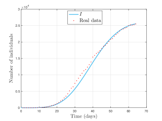
Figure 2: Number of COVID-19 infected individuals $I(t)$, $t\in[0,64]$ days, predicted by model (1), assuming all values of Table 2 – solid green line; real data of Portugal, from 2nd March 2020 to 4th May 2020, from [12] – red points.

In Figure 3, we find the predicted number of hospitalized individuals in Portugal for $t\in[0,64]$, through the mathematical model (1), versus real data from 2nd March 2020 to 4th May 2020, available in [12]. However, the plotted curve $H$, predicted by the proposed mathematical model (1) as given in Figure 3, has a shift of 13 days with respect to reported values of hospitalized individuals in Portugal.

Figure 3: Number of hospitalized individuals $H(t)$, $t\in[0,64]$ days, predicted by model (1), assuming all values of Table 2 – solid green line; real data of Portugal, from 2nd March 2020 to 4th May 2020, from [12] – red points.

The basic reproduction number $R_{0}$, given by (4), takes the value $R_{0}^{*}\simeq 0.95$ for the parameter values of Table 2. The points $(\beta=1.93,R_{0}^{*})$, $(p=0.68,R_{0}^{*})$, $(\omega=1/31,R_{0}^{*})$, and $(m=0.075,R_{0}^{*})$, are marked in Figures 4–7 with the mark $*$.

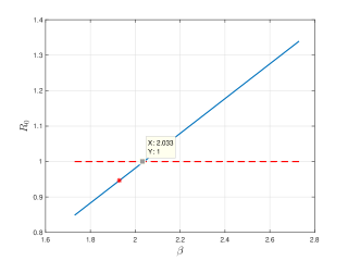
Figure 4: Influence of the parameter $\beta$ in the value of $R_{0}(\beta)$, for $\beta\in[\beta^{*}-0.2,\beta^{*}+0.8]$, where $\beta^{*}$ and all the other parameters take the values of Table 2.

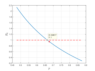
Figure 5: Influence of the parameter $p$ in the value of $R_{0}(p)$, for $p\in[p^{*}-0.2,p^{*}+0.2]$, where $p^{*}$ and all the other parameters take the values of Table 2.

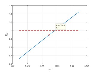
Figure 6: Influence of the parameter $\omega$ in $R_{0}(\omega)$, for $\omega\in[\omega^{*}-0.01,\omega^{*}+0.01]$, where $\omega^{*}$ and all the other parameters take the values of Table 2.

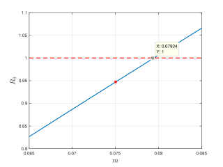
Figure 7: Influence of the parameter $m$ in $R_{0}(m)$, for $m\in[m^{*}-0.01,m^{*}+0.01]$, where $m^{*}$ and all the other parameters take the values of Table 2.

Remark 4.2.

Our SAIQH-like compartmental epidemic model describes very well the evolution of COVID-19 in Portugal. Indeed, the results of the fittings are quite good: the $L^{2}$ error of the fit associated with infected individuals $I$ (see Figure 2) and hospitalized individuals $H$ (see Figure 3), both with respect to the initial population $N_{0}$, are equal to $9.2152e-04$ and $1.6136e-04$, respectively. Moreover, the parameter values we are considering, correspond to a basic reproduction number that is in agreement with the value given by the Portuguese authorities at the end of the three emergency states (cf. page 8 of the report [32]).

We can see that at the end of the 45 days period of state of emergency, Portugal is in a possible turning point situation where the number of new infected individuals can continue to decrease or, in the opposite, if the number of contacts between infected and susceptible individuals increases, the Portuguese epidemiological situation can converge to an endemic equilibrium. However, if social distance and all preventive measures are taken, the spread of corona virus can remain in values for which the Portuguese Health system can answer in an efficient way, has it happened until the date of 4th May, 2020.

5 Conclusions and Discussion

SIR (Susceptible–Infectious–Recovered) type models provide powerful tools to describe and control infection disease dynamics [19, 24, 35]. Recently, several mathematical models have been developed to study the COVID-19 pandemic. These include [27], where the case of Wuhan is addressed; [4], where the COVID-19 epidemic in Morocco is analyzed; [7], which investigates the situation in Costa Rica; as well as several other investigations studying the reality of many other countries: Canada [8], Italy [14], Pakistan [38], etc. Other studies analyze and compare the realities of more than one country: see, e.g., [8], for the cases of China, Italy and France; or [30], for the realities of South Korea, Italy, and Brazil. Typically, the proposed mathematical models fits well the number of confirmed active infected cases with COVID-19. Here we propose a new compartmental model that not only allows to fit well the number of confirmed active infected COVID-19 cases but also fits simultaneously the number of individuals that need to be hospitalized. This is far from being trivial and one should remark that the standard SIR, SEIR, and SEIRQ models, as well as many other extensions found in the literature, do not allow to do this, while our model does. Such novelty is of primordial importance, since it is well known that one crucial point in COVID-19 pandemic is to ensure that the health systems are never overloaded.

We proposed a new compartmental model with the goal to describe the COVID-19 pandemic in Portugal, since its emergence, on 2nd March 2020, till 4th May 4, 2020, when the Portuguese authorities started releasing gradually the country from the severe COVID-19 confinement measures and canceling the very restrictive State of Emergency measures.

Figure 2 shows a strictly increasing function in all the considered time interval, that is, the pandemic continues to propagate, since the peak of infected individuals has not yet been reached at $t=64$. Figure 3 shows a strictly increasing function in an interval $[0,t_{\max})$ and strictly decreasing in the interval of time $(t_{\max},64]$. We conclude that the maximum number of hospitalized individuals has already been reached and despite the fact that the pandemic continues to spread, hospitalization in Portugal is controlled. From Figures 4, 5, 6 and 7, we observe that the famous $R_{0}$ depends linearly on $\beta$, $\omega$ and $m$ parameters, but the same is no longer the case with the $p$ parameter. Furthermore, we can see that as the values of $\beta$, $\omega$ and $m$ increase, the value of $R_{0}$ increases as well. Regarding the parameter $p$, the opposite happens: as the value of $p$ increases, the value of the basic reproduction number $R_{0}$ decreases. Such numerical conclusions make sense considering the meaning of all these parameters (see Table 1) and are in agreement with the analytical results obtained in Section 3.

Concluding, our results show that at the end of the three emergency states declared in Portugal, the country begins 4th May 2020 a possible turning point situation where the number of new infected individuals can continue to decrease or, in the opposite, if the number of contacts between infected and susceptible individuals increases, the Portuguese epidemiological situation can converge to an endemic equilibrium. However, if social distance and all preventive measures continue to be taken, the spread of corona virus can remain in values for which the Portuguese Health system can answer in an efficient way, has it happened until the date of 4th May, 2020. Because the fraction of the population that was infected is very small and nothing is known yet about the herd immunity of the population, there is always the danger that with the gradual return of Portuguese population to the susceptible class, from June and July 2020 on, a very large and rapid increase in disease transmission may result. It means that the possibility of a second wave of COVID-19 in Portugal is not ruled out.

From the theoretical/mathematical point of view, it remains open the study of the local and global stability of the endemic equilibrium. This seems quite difficult. From one side, for the local stability, the computation of the eigenvalues of the Jacobian matrix evaluated at the endemic equilibrium is cumbersome. For the global stability, finding a suitable Lyapunov function is also a difficult task. These are interesting open problems.

References

- [1] K. Allali, S. Harroudi and D. F. M. Torres, Analysis and optimal control of an intracellular delayed HIV model with CTL immune response, Math. Comput. Sci. 12 (2018), no. 2, 111–127. doi:10.1007/s11786-018-0333-9. arXiv:1801.10048
- [2] I. Area, F. Ndaïrou, J. J. Nieto, C. J. Silva and D. F. M. Torres, Ebola model and optimal control with vaccination constraints, J. Ind. Manag. Optim. 14 (2018), no. 2, 427–446. doi:10.3934/jimo.2017054. arXiv:1703.01368
- [3] S. Boccaletti, W. Ditto, G. Mindlin and A. Atangana, Modeling and forecasting of epidemic spreading: The case of COVID-19 and beyond, Chaos, Solitons and Fractals 135, 109–794 (2020). doi:10.1016/j.chaos.2020.109794.
- [4] A. Bouchnita and A. Jebrane, A multi-scale model quantifies the impact of limited movement of the population and mandatory wearing of face masks in containing the COVID-19 epidemic in Morocco, Math. Model. Nat. Phenom. 15 (2020). doi:10.1051/mmnp/2020016.
- [5] F. Brauer and C. Castillo-Chávez, Mathematical models in population biology and epidemiology, Texts in Applied Mathematics, vol. 40, Springer-Verlag, New York (2001). doi:10.1007/978-1-4757-3516-1.
- [6] C. Castillo-Chavez and B. Song, Dynamical models of tuberculosis and their applications, Math. Biosci. Eng. 1 (2004), no. 2, 361–404. doi:10.3934/mbe.2004.1.361.
- [7] L. F. Chaves, L. A. Hurtado, M. R. Rojas, M. D. Friberg, R. M. Rodríguez and M. L. Avila-Aguero, COVID-19 basic reproduction number and assessment of initial suppression policies in Costa Rica, Math. Model. Nat. Phenom. 15 (2020). doi:10.1051/mmnp/2020019.
- [8] V. K. R. Chimmula and L. Zhang, Time series forecasting of COVID-19 transmission in Canada using LSTM networks, Chaos Solitons Fractals 135 (2020), 109864. doi:10.1016/j.chaos.2020.109864.
- [9] Comité Español de Matemáticas, Mathematics against coronavirus, [Online; accessed on 04th May 2020]
- [10] S. Contreras et. al., A multi-group SEIRA model for the spread of COVID-19 among heterogeneous populations, Chaos, Solitions Fractals 136 (2020), 1099325. doi:10.1016/j.chaos.2020.109925.
- [11] N. Crokidakis, COVID-19 spreading in Rio de Janeiro, Brazil: Do the policies of social isolation really work?, Chaos, Solitions Fractals 136 (2020), 109930. doi:10.1016/j.chaos.2020.109930.
- [12] Direção-Geral da Saúde – COVID-19, Ponto de Situação Atual em Portugal. [Online; last accessed on 4th May 2020]
- [13] D. Fanelli and F. Piazza, Analysis and forecast of COVID-19 spreading in China, Italy and France, Chaos Solitons Fractals 134 (2020), 109761. doi:10.1016/j.chaos.2020.109761.
- [14] G. Giordano, F. Blanchini, R. Bruno , P. Colaneri, A. D. Filippo, A. D. Matteo and M. Colaneri, Modelling the COVID-19 epidemic and implementation of population-wide interventions in Italy, Nature Medicine (2020). doi:10.1038/S41591-020-0883-7.
- [15] K. Hattaf and N. Yousfi, Dynamics of SARS-CoV-2 infection model with two modes of transmission and immune response, Math. Biosci. Eng. 17 (2020), no. 5, 5326–5340. doi:10.3934/mbe.2020288.
- [16] H. W. Hethcote, The mathematics of infectious diseases, SIAM Rev. 42 (2000), no. 4, 599–653. doi:10.1137/S0036144500371907.
- [17] Jornal de Negócios, O que fazem os portugueses na quarentena? [Online; accessed on 27th March 2020]
- [18] Y. Kim, S. Lee, C. Chu, S. Choe, S. Hong and Y. Shin, The characteristics of middle eastern respiratory syndrome coronavirus transmission dynamics in South Korea, Osong Public Health Res. Perspect. 7 (2016), no. 1, 49–55. doi:10.1016/j.phrp.2016.01.001.
- [19] B. W. Kooi, M. Aguiar and N. Stollenwerk, Bifurcation analysis of a family of multi-strain epidemiology models, J. Comput. Appl. Math. 252 (2013), 148–158. doi:10.1016/j.cam.2012.08.008.
- [20] V. Lakshmikantham, S. Leela and A. A. Martynyuk, Stability analysis of nonlinear systems, Monographs and Textbooks in Pure and Applied Mathematics, Marcel Dekker, Inc., New York (1989).
- [21] A. P. Lemos-Paião, C. J. Silva and D. F. M. Torres, An epidemic model for cholera with optimal control treatment, J. Comput. Appl. Math. 318 (2017), 168–180. doi:10.1016/j.cam.2016.11.002. arXiv:1611.02195
- [22] A. P. Lemos-Paião, C. J. Silva, D. F. M. Torres and E. Venturino, Optimal Control of Aquatic Diseases: A Case Study of Yemen’s Cholera Outbreak, J. Optim. Theory Appl. 185 (2020), no. 3, 1008–1030. doi:10.1007/s10957-020-01668-z. arXiv:2004.07402
- [23] B. F. Maier and D. Brockmann, Effective containment explains sub-exponential growth in confirmed cases of recent COVID-19 outbreak in China, Science 368 (2020), 742–746. doi:10.1126/science.abb4557.
- [24] A. Mallela, S. Lenhart and N. K. Vaidya, HIV-TB co-infection treatment: modeling and optimal control theory perspectives, J. Comput. Appl. Math. 307 (2016), 143–161. doi:10.1016/j.cam.2016.02.051.
- [25] J. Matovinovic, A short history of quarantine (Victor C. Vaughan), Univ. Mich. Med. Cent. J. 35 (1969), no. 4, 224–228.
- [26] A. A. Mohsen, H. F. Al-Husseiny, X. Zhou and K. Hattaf, Global stability of COVID-19 model involving the quarantine strategy and media coverage effects, AIMS Public Health 7 (2020), no. 3, 587–605. doi:10.3934/publichealth.2020047.
- [27] F. Ndaírou, I. Area, J. J. Nieto and D. F. M. Torres, Mathematical modeling of COVID-19 transmission dynamics with a case study of Wuhan, Chaos Solitons Fractals 135 (2020), 109846. doi:10.1016/j.chaos.2020.109846. arXiv:2004.10885
- [28] PORDATA: Base de Dados de Portugal Contemporâneo, Alunos matriculados no ensino pré-escolar: total e por subsistema de ensino, [Online; accessed on 20th March 2020]
- [29] PORDATA: Base de Dados de Portugal Contemporâneo, Números de Portugal: Quadro-resumo. [Online; accessed on 20th March 2020]
- [30] R. F. Reis, B. de Melo Quintela, J. de Oliveira Campos, J. M. Gomes, B. M. Rocha, M. Lobosco and R. Weber dos Santos, Characterization of the COVID-19 pandemic and the impact of uncertainties, mitigation strategies, and underreporting of cases in South Korea, Italy, and Brazil, Chaos Solitons Fractals 136 (2020), 109888. doi:10.1016/j.chaos.2020.109888.
- [31] República Portuguesa: XXII Governo, Comunicação – Documentos, [Online; accessed on 13th March 2020]
- [32] República Portuguesa: XXII Governo, Comunicação – Documentos, [Online; accessed on 22nd July 2020]
- [33] S. Rosa and D. F. M. Torres, Optimal control and sensitivity analysis of a fractional order TB model, Stat. Optim. Inf. Comput. 7 (2019), no. 3, 617–625. doi:10.19139/soic.v7i3.836. arXiv:1812.04507
- [34] RTP Notícias, COVID-19, [Online; accessed on 19th March 2020]
- [35] C. J. Silva and D. F. M. Torres, A TB-HIV/AIDS coinfection model and optimal control treatment, Discrete Contin. Dyn. Syst. 35 (2015), no. 9, 4639–4663. doi:10.3934/dcds.2015.35.4639. arXiv:1501.03322
- [36] E. Tognotti, Lessons from the History of Quarantine, from Plague to Influenza A, Emerg. Infect. Dis. 19 (2013), no. 2, 254–259. doi:10.3201/eid1902.120312.
- [37] P. van den Driessche and J. Watmough, Reproduction numbers and sub-threshold endemic equilibria for compartmental models of disease transmission, Math. Biosci. 180 (2002), 29–48. doi:10.1016/S0025-5564(02)00108-6.
- [38] M. Yousaf, S. Zahir, M. Riaz, S. M. Hussain and K. Shah, Statistical analysis of forecasting COVID-19 for upcoming month in Pakistan, Chaos Solitons Fractals 138 (2020), 109926. doi:10.1016/j.chaos.2020.109926.
- [39] World Health Organization, Q&A on coronaviruses (COVID-19), [Online; available since 09th March 2020]
- [40] Worldometer, Coronavirus Symptoms (COVID-19). [Online; available since 29th February 2020]
- [41] H. Zine, A. Boukhouima, E. M. Lotfi, M. Mahrouf, D. F. M. Torres and N. Yousfi, A stochastic time-delayed model for the effectiveness of Moroccan COVID-19 deconfinement strategy, Math. Model. Nat. Phenom. 15 (2020), Art. 50, 14 pp. doi:10.1051/mmnp/2020040. arXiv:2010.16265