Extending Charged Holographic Rényi Entropy

Abstract

Motivated by extended black hole thermodynamics, we generalize the Rényi entropy of charged holographic conformal field theories (CFTs) in $d$-dimensions. Specifically, following Johnson:2018bma , we extend the quench description of the Rényi entropy of globally charged holographic CFTs by including pressure variations of charged hyperbolically sliced anti de Sitter black holes. We provide an exhaustive analysis of the new type of charged Rényi entropy, where we find an interesting interplay between a parameter controlling the pressure of the black hole and its charge. A field theoretic interpretation of this extended charged Rényi entropy is given. In particular, in $d=2$, where the bulk geometry becomes the charged Bañados, Teitelboim, Zanelli black hole, we write down the extended charged Rényi entropy in terms of the twist operators of the charged field theory. An area law prescription for the extended Rényi entropy is formulated. We comment on several avenues for future work, including how global charge conservation relates to black hole super-entropicity.

1 Introduction

With the advent of AdS/CFT, it has become clear there is a deep interplay between gravity and information theory. This realization is encapsulated by an entropy-area relation known as the Ryu-Takayanagi (RT) prescription Ryu:2006bv :

$$S_{\text{EE}}^{A}=\frac{\mathcal{A}(\gamma_{A})}{4G_{N}}\;.$$ (1)

Here $S^{A}_{\text{EE}}$ is the entanglement entropy of a conformal field theory (CFT) reduced to a region $A$ on the $d$-dimensional boundary of an asymptotically $(d+1)$-dimensional AdS (bulk) spacetime, and $\mathcal{A}(\gamma_{A})$ is the area of a static bulk minimal surface $\gamma_{A}$ that is homologous to boundary region $A$. The RT formula (1) and its covariant version Hubeny:2007xt provide an information theoretic interpretation of the Bekenstein-Hawking entropy-area relation Bekenstein:1972tm ; Hawking:1974rv ; Hawking:1974sw . Indeed, in an early attempt to provide a derivation of holographic entanglement entropy, Casini, Huerta, and Myers (CHM), showed that the entanglement entropy of a holographic CFT reduced to a ball in Minkowski space is equal to the thermodynamic entropy of a massless, hyperbolically sliced AdS-Schwarzschild black hole Casini:2011kv . In this way, black holes provide a throughline connecting gravity, thermodynamics, and information.

For field theories, rather than computing the entanglement entropy directly one instead computes the Rényi entropy $S_{q}$,

$$S_{q}=\frac{1}{1-q}\log[\text{tr}(\rho_{A}^{q})]\;,$$ (2)

where $\rho_{A}$ is the reduced density matrix of the CFT, and $q$ is the Rényi index. The entropy $S_{q}$ can be used to calculate the entanglement entropy: In the limit $q\to 1$, $S_{1}=-\text{tr}(\rho\log\rho)$, the von Neumann entropy. The Renyí entropy, in this way, is more fundamental than the entanglement entropy. Moreover, other limits of $S_{q}$ provide additional insight into the nature of the entanglement spectrum. In the large $q$ limit (2) yields the largest eigenvalue $\lambda$ of $\rho_{A}$, $S_{\infty}=-\log(\lambda)$ (the min-entropy), and as $q\to 0$ we have $S_{0}=\log(d)$, where $d$ is the number of nonvanishing eigenvalues of $\rho_{A}$ (the Hartley entropy) Headrick:2010zt . Thus, $S_{q}$ is an important diagnostic probe in information theory and condensed matter physics.

When the field theory in question carries a conserved (global) charge, the entanglement Rényi entropy $S_{q}$ is replaced with a grand canonical version of (2),

$$S_{q}(\mu)=\frac{1}{1-q}\log\text{tr}\left(\rho_{A}\frac{e^{\mu Q_{A}}}{n_{A}(\mu)}\right)^{q}\;,$$ (3)

where $\mu$ is a ‘chemical potential’ conjugate to the charge $Q_{A}$ confined to $A$, and $n_{A}(\mu)\equiv\text{tr}[\rho_{A}e^{\mu Q_{A}}]$ properly normalizes the ‘charged’ reduced state $\rho_{A}e^{\mu Q_{A}}$. The charged Rényi entropy $S_{q}(\mu)$ therefore encodes how the entanglement between $A$ and its complement depends on the charge.

For CFTs with holographic duals, both the charged and uncharged entropies $S_{q}$ for general $q$ can be related to the thermodynamics of black holes and explicitly evaluated. This is accomplished in the following way Casini:2011kv . Take the CFT ground state $\rho_{R}=e^{-K_{R}}$ reduced to a ball of radius $R$ in $d$-dimensional Minkowski space with $K_{R}$ being the modular Hamiltonian generating a local modular flow in the causal domain of the ball. A judicious coordinate transformation takes the Minkowski background to the geometry of $\mathbb{R}\times\mathbb{H}^{d-1}$ with $\mathbb{H}^{d-1}$ a hyperbolic plane of size $R\equiv L_{0}$, up to a conformal factor, which may be eliminated with a conformal transformation. The reduced state $\rho_{R}$ is not invariant under the conformal transformation. Letting $U$ be the unitary operator acting on the CFT Hilbert space that implements the conformal transformation, we write the CHM map

$$\rho_{R}=e^{-K_{R}}=U^{\dagger}\left(\frac{e^{-\beta H_{\tau}}}{Z}\right)U\;,$$ (4)

where $H_{\tau}$ is the Hamiltonian generating time $\tau$ translations in the hyperbolic space, and $\beta$ is the inverse temperature $T_{0}=1/(2\pi L_{0})$. Since the von Neumann entropy is invariant under unitary transformations, this means the entanglement entropy across the ball $S_{\text{EE}}=-\text{tr}(\rho_{R}\log\rho_{R})$ is mapped to a thermal entropy on the hyperbolic background. With $\rho_{R}$ in Gibbs form, it is then straightforward to rewrite (2) as a “quench” of the Helmholtz free energy $F(T)$ baez:2011

$$S_{q}=-\frac{1}{\Delta T}[F(T_{0})-F(T_{0}/q)]=\frac{1}{\Delta T}\int^{T_{0}}_{T_{0}/q}S(T)dT\;,$$ (5)

where $S=-\partial F/\partial T|_{V}$ and with $\Delta T=T_{0}-T_{0}/q$. In this sense, the Rényi entropy is an appropriately normalized measure of the free energy difference $\Delta F$ between the system at temperature $T_{0}$ and the system at temperature $T_{0}/q$, assuming the pressure is held fixed. The connection to black hole physics is made with the aid of the CHM map (4), in which the entropy $S(T)$ is replaced by the thermal entropy of a black hole with hyperbolic horizon Hung:2011nu . In the charged Rényi case, the charged CFT is dual to a charged black hole Belin:2013uta .

Due to the importance of both charged and uncharged Rényi entropies, any potential generalization is of interest. For holographic field theories a natural generalization presents itself, motivated by the program of extended black hole thermodynamics Kastor:2009wy ; Kastor:2010gq ; Dolan:2010ha ; Dolan:2012jh ; Kubiznak:2016qmn , where the cosmological constant $\Lambda$ present in $\text{AdS}_{d+1}$ black hole backgrounds is interpreted as a pressure, $p=-\frac{\Lambda}{8\pi G_{N}}=\frac{d(d-1)}{16\pi G_{N}L^{2}}$, with $L$ being the AdS radius. Consequently, an AdS black hole has its mass $M$ identified with the enthalpy $H$ of a thermodynamic system and the first law of black hole thermodynamics is extended to $dH=TdS+Vdp$. The quantity $V=\left(\frac{\partial H}{\partial p}\right)_{S}$ is the conjugate variable to the pressure and is known as the ‘thermodynamic volume’, since in static spacetimes of four dimensions and higher it is the naive geometric volume of the black hole, while for, e.g., rotating systems it includes terms dependent on their spin.

According to the extended framework of black hole thermodynamics, it is then natural to extend the quench form of $S_{q}$ given in (5), by relaxing the condition of fixed pressure. Using the first law $\Delta G=V\Delta p-S\Delta T$, we simply replace $\Delta F$ with a difference in Gibbs free energies $\Delta G$ evaluated at different temperatures and pressures Johnson:2018bma

$$S_{q,b}\equiv-\frac{G(p_{0},T_{0})-G(b^{2}p_{0},T_{0}/q)}{(\Delta T-V_{0}\Delta p/S_{0})}=\frac{1}{(\Delta T-V_{0}\Delta p/S_{0})}\int^{T_{0}}_{T_{0}/q}S(T)\left(1-\frac{V}{S}\frac{dp}{dT}\right)dT\;,$$ (6)

where $\Delta p=p_{0}-b^{2}p_{0}$, with $b$ another integer ‘index’ that plays a similar role as $q$. In the limit $b\to 1$ the usual Rényi entropy is recovered; the limit $q\to 1$ leads to a new kind of Rényi entropy $S_{b}$ whose interpretation is still largely mysterious. Nonetheless, as first shown in Johnson:2018bma , the generalized Rényi entropy $S_{q,b}$ can be explicitly computed, and has a number of interesting properties. In particular, in the $d=2$ case, the index $b$ can be seen to undo the $q$-sheets used in the replica trick when calculating $S_{q}$, granting $S_{q,b}$ a field theory interpretation arising from a generalization of the CHM map (4),

$$\rho^{(b)}_{R}=U^{\dagger}\left(\frac{e^{-(H_{\tau}+b^{2}p_{0}V_{0})/T_{0}}}{Z(T_{0},p_{0})}\right)U\;,$$ (7)

such that

$$S_{q,b}=\frac{1}{[(1-q)-q(d-1)(b^{2}-1)/2]}\log\left[\text{tr}(\rho^{(b)}_{R})^{q}\right]\;.$$ (8)

This suggests $S_{1,b}$ can be computed via the replica trick as $\rho_{w}^{b}\equiv\rho_{R}^{(b)}$ for some other density matrix $\rho_{w}$ via a Euclidean path integral over a $b$ sheeted manifold. In this way, $b$ plays a role very similar to the traditional Rényi index $q$.

In this article, following Johnson:2018bma , we extend the charged holographic Rényi entropy (3) first explored in Belin:2013uta . Our motivation of extending (3) is three fold. Firstly, generalizing $S_{q}(\mu)$ to $S_{q,b}(\mu)$ provides a new entry in the holographic dictionary, in which we deepen the connection between entanglement and black hole entropy. Secondly, as the charged Rényi entropy plays an important role in studying phase transitions of holographic superconductors Belin:2014mva , it’s single parameter deformation $S_{q,b}(\mu)$ may shed new light into the phases of charged black hole systems. Finally, as with the uncharged generalized Rényi entropy, since $S_{q,b}(\mu)$ is computed starting on the gravity side, its field theoretic interpretation may provide additional insight into the replica calculation of charged Rényi entropies more generally.

The outline of this article is as follows. For completeness, in Section 2 we briefly review the construction and computation of charged holographic Rényi entropies for CFT states dual to charged black holes. Section 3 is devoted to extending the charged Rényi entropy, where we specifically consider CFT states dual to charged AdS black holes in four spacetime dimensions and higher. We find an interesting interplay between the chemical potential $\mu$ and parameter $b$, and briefly analyze the behavior of $S_{q,b}$ for imaginary chemical potentials $i\mu_{E}$. In Section 4 we provide a partial discussion of the field theory interpretation of $S_{q,b}$, including a generalization of the holographic calculation for the conformal dimension of twist operators inserted at the entangling surface. The geometry of charged $\text{AdS}_{d+1}$ black hole systems changes dramatically when $d=2$, in which case the dual Rényi entropy requires a more careful treatment Belin:2013uta . In Section 5 we extend the charged Rényi entropy for CFTs dual to the charged Bañados, Teitelboim, Zanelli (BTZ) black hole Martinez:1999qi , where we provide a more precise field theoretic interpretation of $b$. In Section 6 we provide an area law formulation of the extended Rényi entropy, akin to Dong’s proposal for $S_{q}$ Dong:2016fnf . We conclude and discuss potential avenues for future work in Section 7.

2 Charged Holographic Rényi Entropy: Review

When we consider quantum field theories with a conserved global charge, the Renyí entropy is generalized to a charged Rényi entropy, given in (3), where $\mu$ is a ‘chemical potential’ and $Q_{A}$ is the charge confined to the subsystem of interest Belin:2013uta . As with ordinary Renyí entropies, the charged quantities can be evaluated using the replica trick, involving a Euclidean path integral on a $q$-sheeted geometry with twist operators $\sigma_{q}$ imposed at the boundary points of the cuts of the sheets where the entangling surface lives. A new ingredient is added, however, requiring a Wilson loop of the background gauge field $B$ associated with charge $Q_{A}$ to the entangling surface, thereby generalizing the twist operator to include a magnetic flux proportional to $\mu$. The addition of a Wilson line about the Euclidean time circle is in fact a standard feature when including a chemical potential $\mu$ in the usual Euclidean path integral representation of a grand canonical thermal ensemble.

When the quantum field theory is a CFT, the charged Rényi entropy can be evaluated expressed using the quench (5), where the CHM map (4) generalizes to

$$\rho_{A}\frac{e^{\mu Q_{A}}}{n_{A}(\mu)}=U^{-1}\left(\frac{e^{-H_{\tau}/T_{0}+\mu Q_{A}}}{Z(T_{0},\mu)}\right)U\;,\quad\rho_{\text{therm}}=\frac{e^{-H_{\tau}/T_{0}+\mu Q_{A}}}{Z(T_{0},\mu)}\;.$$ (9)

Here $Z(T_{0},\mu)$ is the thermal partition function associated with $\rho_{\text{therm}}$. The quench (5) generalizes straightforwardly to

$$S_{q}(\mu)=\frac{1}{1-q}\log\frac{Z(T_{0}/q,\mu)}{Z(T_{0},\mu)^{q}}=\frac{q}{q-1}\frac{1}{T_{0}}\int_{T_{0}/q}^{T_{0}}S(T,\mu)dT\;,$$ (10)

where we used that the free energy $F(T,\mu)$ is related to the partition function via $Z(T,\mu)=\exp(-F(T,\mu)/T_{0})$, and that the thermal entropy of the CFT is $S(T,\mu)=-\partial F/\partial T|_{V,\mu}$.

For holographic CFTs the thermal entropy $S$ is equivalent to the horizon entropy of an AdS black hole with a hypebolically sliced horizon. Via the AdS/CFT dictionary, the global symmetry due to the conserved charge $Q_{A}$ in the boundary CFT translates to a gauge field $A$ in the dual gravity theory, such that the AdS black hole is (electrically) charged. In particular, the $d+1$-dimensional bulk theory is described by an Einstein-Maxwell action

$$I_{EM}=\frac{1}{16\pi G_{N}}\int d^{d+1}x\sqrt{-g}\left(R+\frac{d(d-1)}{L^{2}}-\frac{\ell^{2}_{\ast}}{4}F_{\mu\nu}F^{\mu\nu}\right)\;,$$ (11)

where $\ell_{\ast}$ is the electromagnetic coupling. This theory admits charged topological black holes with metric

$$ds^{2}=-f(r)d\tau^{\prime 2}+f^{-1}(r)dr^{2}+r^{2}(du^{2}+\sinh^{2}(u)d\Omega_{d-2}^{2})\;,$$ (12)

with

$$f(r)=\frac{r^{2}}{L^{2}}-1-\frac{m}{r^{d-2}}+\frac{q_{e}^{2}}{r^{2d-4}}\;.$$ (13)

The horizon $r_{h}$ is located at the largest root of $f(r_{h})=0$. The gauge field $A$ is

$$A=\left(\sqrt{\frac{2(d-1)}{(d-2)}}\frac{q_{e}}{\ell_{\ast}}\right)\left(\frac{1}{r_{h}^{d-2}}-\frac{1}{r^{d-2}}\right)d\tau^{\prime}\;.$$ (14)

The chemical potential $\mu$ is fixed by demanding $A=0$ at the horizon,

$$\mu=2\pi\sqrt{\frac{2(d-1)}{(d-2)}}\frac{q_{e}}{\ell_{\ast}r_{h}^{d-2}}\;.$$ (15)

Writing the blackening factor $f(r)$ in terms of the horizon radius $r_{h}$,

$$f(r)=\frac{r^{2}}{L^{2}}-1+\frac{q^{2}_{e}}{r^{2d-4}}-\left(\frac{r_{h}}{r}\right)^{d-2}\left(\frac{r_{h}^{2}}{L^{2}}-1+\frac{q^{2}_{e}}{r_{h}^{2d-4}}\right)\;,$$ (16)

the temperature of the black hole is simply

$$\begin{split}T&=\frac{f^{\prime}(r_{h})}{4\pi}=\frac{1}{4\pi Lx}\left(dx^{2}-(d-2)-\frac{(d-2)^{2}}{2(d-1)}\left(\frac{\mu\ell_{\ast}}{2\pi}\right)^{2}\right)\end{split}\;,$$ (17)

with $x\equiv r_{h}/L$. In the neutral limit, when the black hole is massless $L=L_{0}$ such that $x=1$ and $T_{0}=1/(2\pi L_{0})$. The thermal entropy is the usual Bekenstein-Hawking entropy

$$S_{\text{BH}}=\frac{w_{d-1}L^{d-1}}{4G_{N}}x^{d-1}=\frac{L^{d-1}x^{d-1}}{4G_{N}}\Omega_{d-2}\int^{\infty}_{0}du\sinh^{d-2}(u)\;,$$ (18)

where $w_{d-1}$ is the volume of $\mathbb{H}^{d-1}$ parameterized by coordinate $u\in\mathbb{R}_{+}$, and $\Omega_{d-2}$ is the volume of a unit sphere $S^{d-2}$.

The charged Renyí entropy is then computed via (10), with the thermal entropy being replaced by the horizon entropy Belin:2013uta :

$$\begin{split}S_{q}(\mu)&=\frac{q}{q-1}\frac{1}{T_{0}}\int_{x_{q}}^{x_{1}}S(x,\mu)\frac{dT}{dx}dx\\ &=\frac{q}{q-1}\frac{S_{EE}}{2}\left[x_{1}^{d-2}\left(1+\frac{(d-2)}{2(d-1)}\left(\frac{\mu\ell_{\ast}}{2\pi}\right)^{2}+x_{1}^{2}\right)-x_{q}^{d-2}\left(1+\frac{(d-2)}{2(d-1)}\left(\frac{\mu\ell_{\ast}}{2\pi}\right)^{2}+x_{q}^{2}\right)\right]\;.\end{split}$$ (19)

Here $x_{q}$ is the largest solution to $T(x_{q},\mu)=T_{0}/q$, given by

$$x_{q}=\frac{1}{qd}\left[1+\sqrt{1+q^{2}d(d-2)+\frac{q^{2}d(d-2)^{2}}{2(d-1)}\left(\frac{\mu\ell_{\ast}}{2\pi}\right)^{2}}\right]\;.$$ (20)

Equation (19) is the charged holographic Rényi entropy for CFTs in dimension $d\geq 3$. We emphasize by $S_{EE}$ we really mean the entanglement entropy for the neutral CFT, $S_{EE}(\mu=0)$. Holographically this is given by Casini:2011kv

$$S_{\text{EE}}=\left(\frac{2\Gamma(d/2)\Omega_{d-2}}{\pi^{d/2-1}}\right)a_{d}^{\ast}\int^{y_{\text{max}}}_{0}dy\frac{y^{d-2}}{\sqrt{1+y^{2}}}\;,$$ (21)

where $y=\sinh(u)$ and $y_{\text{max}}$ is a cutoff to regulate the UV divergence of the entanglement entropy due to correlations close to the entangling surface. The $L_{0}$ dependent factor has been replaced by the generalized central charge $a^{\ast}_{d}$ Myers:2010tj

$$a^{\ast}_{d}=\frac{\pi^{d/2-1}L_{0}^{d-1}}{8\Gamma(d/2)G_{N}}\;.$$ (22)

The charged von Neumann entropy $S_{EE}(\mu)$ is simply given by the $q\to 1$ limit of $S_{q}(\mu)$. As explored in Belin:2013uta , there are other limits of (19) that are of interest. In particular, the $q\to 0$ limit is independent of $\mu$ and matches the same limit in the uncharged case, while the large $\mu$ behavior of $S_{q}(\mu)$ (at fixed $q$) is completely independent of the index $q$.

Charged Rényi entropies constructed from an imaginary chemical potential are also of interest. This can be done on the field theory side by analytically continuing $\mu\to i\mu_{E}$ for $\mu_{E}$ real. There is no issue with this analytic continuation procedure near $\mu=0$, however, one can encounter singularities along the imaginary $\mu$-axis. On the gravity side, the analytic continuation in $\mu$ corresponds to the continuation in the electric charge of the black hole $q_{e}\to iq_{e}^{E}$. There is no real problem with this except when $\mu_{E}$ exceeds the upper bound $\mu_{E}^{2}\leq\frac{8\pi^{2}(d-1)}{d-2}\left(\frac{1}{\ell_{\ast}}\right)^{2}\left(1+\frac{1}{d(d-2)q^{2}}\right)$, where $x_{q}$ goes imaginary. Consequently, the event horizon of the black hole disappears leaving a naked singularity.

3 Physical Generalization of Charged Rényi Entropy

3.1 Extended Thermodynamics of Hyperbolic AdS-RN Black Hole

The above holographic computations kept the AdS length scale $L$ fixed at $L_{0}$. In extended black hole thermodynamics Kastor:2009wy ; Kastor:2010gq ; Dolan:2010ha ; Dolan:2012jh ; Kubiznak:2016qmn , a fixed length $L_{0}$ corresponds to a fixed thermodynamic pressure $p_{0}=\frac{d(d-1)}{16\pi G_{N}L_{0}^{2}}$. Equivalently, then, the quench (5) is understood as a difference in Gibbs free energies at different temperatures, but fixed pressures. It is thus natural to extend the Rényi entropy in (5) by allowing the pressure to vary, exploiting the enlarged framework of extended black hole thermodynamics. This was first accomplished in Johnson:2018bma .

Similarly, we can extend the charged Rényi entropy (19) by exploiting the extended thermodynamics of hyperbolic AdS-RN black holes. The extended thermodynamics for this system has not yet appeared in the literature, however, it is straightforward to work out. We already have the temperature and entropy, (17) and (18), respectively. The mass $M$ of the system, interpreted as the enthalpy in the enlarged framework, may be determined using the quasilocal approach of Brown and York Brown:1992br adapted to an asymptotically AdS background

$$M=-\frac{(d-1)w_{d-1}L^{d-2}}{16\pi G_{N}}x^{d-2}\left(1-x^{2}-\frac{(d-2)}{2(d-1)}\left(\frac{\mu\ell_{\ast}}{2\pi}\right)^{2}\right)\;.$$ (23)

This expression also matches calculations using the Euclidean path integral with a counterterm, first developed in Balasubramanian:1999re ; Emparan:1999pm for specific spacetime dimensions. The electric potential $\Phi_{e}$ is defined by

$$\Phi_{e}=A_{t}|_{r\to\infty}-A_{t}|_{r\to r_{h}}=\frac{q_{e}}{\ell_{\ast}r_{h}^{d-2}}\sqrt{\frac{2(d-1)}{(d-2)}}=\frac{\mu}{2\pi}\;,$$ (24)

and the total electric charge $Q$ is,

$$Q=\frac{w_{d-1}}{16\pi G_{N}}(d-2)\sqrt{\frac{2(d-1)}{(d-2)}}\ell_{\ast}q_{e}=(d-2)\frac{w_{d-1}L^{d-2}}{16\pi G_{N}}x^{d-2}\frac{\mu\ell_{\ast}^{2}}{2\pi}\;.$$ (25)

From the mass $M$ we find that the thermodynamic volume is

$$V\equiv\left(\frac{\partial M}{\partial p}\right)_{S,Q}=\frac{w_{d-1}}{d}r_{h}^{d}=\frac{4G_{N}}{d}r_{h}S_{\text{BH}}\;,$$ (26)

just as in the uncharged case. Notice that the thermodynamic volume of the charged black hole is the naive geometric volume. In fact, since the entropy only depends on the horizon radius $r_{h}$, we may conclude that paths of constant volume $V$ (isochores) are equivalent to paths of constant entropy $S_{\text{BH}}$ (adiabats) in the entire $(p,V)$ plane. This matches the uncharged hyperbolic black hole Johnson:2018amj , as well as static AdS black holes in general Johnson:2014yja . As we will observe later, this behavior does not hold for $d=2$ charged AdS black holes.

The Gibbs free energy is

$$G=M-TS-\Phi_{e}Q\;.$$ (27)

After some minor algebra we have

$$\begin{split}G(x,L)&=-\frac{w_{d-1}L^{d-2}}{16\pi G_{N}}x^{d-2}\left[1+\frac{(d-2)}{2(d-1)}\left(\frac{\mu\ell_{\ast}}{2\pi}\right)^{2}+x^{2}\right]\;.\end{split}$$ (28)

At fixed potential $\mu$, the hyperbolic AdS-RN black hole shares many of the same qualitative features as their neutral cousins. For example, the pressure $p$ for the $M=0$ curve has the same functional dependence of $V$ as shown in Johnson:2018amj

$$p(M=0)=\frac{\kappa}{V^{2/d}}\left[1-\frac{(d-2)}{2(d-1)}\left(\frac{\mu\ell_{\ast}}{2\pi}\right)^{2}\right]\;,\quad\kappa\equiv\frac{d(d-1)}{16\pi G_{N}}\left(\frac{w_{d-1}}{d}\right)^{2/d}\;.$$ (29)

Similarly, the zero temperature curve in the $(p,V)$ plane follows

$$p(T=0)=\left(\frac{d-2}{d}\right)\left(1+\frac{d(d-2)}{2(d-1)}\left(\frac{\mu\ell_{\ast}}{2\pi}\right)^{2}\right)\frac{\kappa}{V^{2/d}}\;.$$ (30)

Consequently, the $p(M=0)$ and $p(T=0)$ curves never coincide with each other such that the zero temperature curve is always below the massless curve. Thus, there is an entire region within the $(p,V)$ plane below the massless curve, where the mass of the black hole is negative.

The field theory interpretation of the curves in the $(p,V)$ plane are also largely the same as the neutral case Johnson:2018amj , when $\mu$ is held fixed. To summarize, points on the massless curve correspond to CFT vacuum states reduced to the ball in Minkowski space, in which moving up to higher $p$ along the curve is correlated with going deeper into the IR, integrating out UV field theory degrees of freedom, equivalent to an RG flow in the dual CFT. Moreover, perturbations up and to the right of the massless curve correspond to CFT states dual to massive charged black holes. In particular, perturbations at fixed pressure correspond to perturbing the ground state of a fixed CFT (such that the extended first law of thermodynamics is dual to the extended first law of entanglement Blanco:2013joa ; Wong:2013gua ), while vertical changes, keeping volume fixed, is equivalent to keeping the entanglement entropy fixed, but moving to a different CFT with a central charge $a_{d}^{\ast}$ with fewer UV degrees of freedom. Moving below the massless curve in the $(p,V)$, interestingly, describes CFT states with negative energy density such that the perturbed state is less entangled than the unperturbed state Blanco:2013lea ; Bianchi:2014qua ; Rosso:2018yax ; Rosso:2019lsm .

3.2 Extended Charged Rényi Entropy

Let us now exploit the extended thermodynamics of our black hole system to generalize the charged Rényi entropy (19). First notice that as in the uncharged case Johnson:2018bma the difference in Helmholtz free energies appearing in the quench (10) can be replaced with a difference in Gibbs free energies, using (28). Keeping $L$ fixed, we see

$$S_{q}(\mu)=-\frac{1}{\Delta T}[G(x_{1},L)-G(x_{q},L)]$$ (31)

recovers the charged Rényi entropy (19).

To extend the charged Rényi entropy we simply allow for pressure changes, such that $L_{0}$ changes to $L_{0}/b$. Then, with $\Delta T\equiv T_{0}-T_{0}/q$ and $\Delta p\equiv\frac{d(d-1)}{16\pi G_{N}}\frac{1}{L_{0}^{2}}(1-b^{2})\;,\quad\frac{V_{0}}{S_{0}}=\frac{4G_{N}L_{0}x_{11}}{d}$,

$$\begin{split}S_{q,b}(\mu)&=-\frac{1}{(\Delta T-V_{0}\Delta p/S_{0})}[G(x_{11},L_{0})-G(x_{qb},L_{0}/b)]\\ &=q\frac{S_{EE}}{2}\frac{\biggr{\{}x_{11}^{d-2}\left(1+\frac{(d-2)}{2(d-1)}\left(\frac{\mu\ell_{\ast}}{2\pi}\right)^{2}+x_{11}^{2}\right)-\left(\frac{x_{qb}}{b}\right)^{d-2}\left(1+\frac{(d-2)}{2(d-1)}\left(\frac{\mu\ell_{\ast}}{2\pi}\right)^{2}+x_{qb}^{2}\right)\biggr{\}}}{[q-1+q(d-1)(b^{2}-1)x_{11}/2]}\;,\end{split}$$ (32)

where

$$x_{qb}=\frac{1}{qbd}\left[1+\sqrt{1+q^{2}b^{2}d(d-2)+\frac{q^{2}b^{2}d(d-2)^{2}}{2(d-1)}\left(\frac{\mu\ell_{\ast}}{2\pi}\right)^{2}}\right]\;.$$ (33)

which is found by setting $T_{0}/q=T(\mu,x_{qb})$ and solving for $x_{qb}$. In the neutral limit $\mu=0$, we recover the result from Johnson:2018bma , where $x_{11}=1$. Also observe $\lim_{b\to 1}S_{q,b}(\mu)$ reduces to $S_{q}(\mu)$ in (19). When $q\to 1$, we have a genuine new kind of entropy to study $S_{1,b}(\mu)$, which we will do so in detail momentarily. Notice, moreover that when $q,b\neq 1$, we have $S_{q,b}(\mu)$ diverges when the index $q$ takes the special value $q_{c}$:

$$q_{c}=\frac{2}{(d-1)(b^{2}-1)x_{11}+2}\;,$$ (34)

for which $b>1$ corresponds to $q_{c}<1$, just as in the neutral case.

Let’s now consider some important limits of our generalization of the charged Renyí entropy $S_{q,b}(\mu)$. It is useful to have

$$\lim_{q\;\text{or}\;b\to 0}x_{qb}\to\frac{2}{qbd}\;,$$ (35)

and

$$\lim_{q\,\text{or}\,b\to\infty}x_{qb}\to\sqrt{\frac{(d-2)}{d}}\sqrt{1+\frac{(d-2)}{2(d-1)}\left(\frac{\mu\ell_{\ast}}{2\pi}\right)^{2}}\equiv x_{\infty}\;,$$ (36)

the former of which matches the uncharged case Johnson:2018bma . We will also be interested in the large $\mu$ limit:

$$\lim_{\mu\to\infty}x_{qb}\to\sqrt{\frac{(d-2)^{2}}{2d(d-1)}}\left(\frac{\mu\ell_{\ast}}{2\pi}\right)\;.$$ (37)

To take the $q,b\to 1$ limits of $S_{q,b}$ the following are useful to know

$$\frac{dx_{qb}}{dq}=-\frac{x_{qb}}{q}\frac{1}{[qbdx_{qb}-1]}\;,\quad\frac{dx_{qb}}{db}=-\frac{x_{qb}}{b}\frac{1}{[qbdx_{qb}-1]}\;.$$ (38)

The limits $q\to 1$ and $b\to 1$ commute such that

$$S_{1,1}(\mu)\equiv S_{EE}(\mu)=\frac{1}{2}S_{EE}\frac{(d-2)x_{11}^{d-2}}{dx_{11}-1}\left(1+\frac{(d-2)}{2(d-1)}\left(\frac{\mu\ell_{\ast}}{2\pi}\right)^{2}+\frac{dx_{11}^{2}}{d-2}\right)\;.$$ (39)

When $\mu=0$ we recover $S_{EE}(\mu)=S_{EE}$, where $x_{11}=1$. This means we will observe different behavior between $S_{q,b}(\mu)/S_{EE}(\mu)$ and $S_{q,b}(\mu)/S_{EE}(0)$, as can be seen in Figure 1 and Figure 2. Except when $\mu=0$, we consider $S_{q,b}(\mu)/S_{EE}(\mu)$ the proper normalization, in that all curves meet at $q=b=1$.

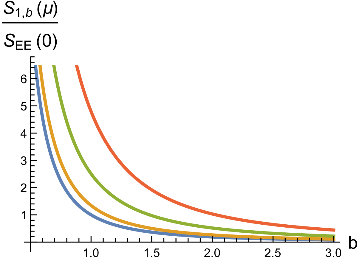
(a)

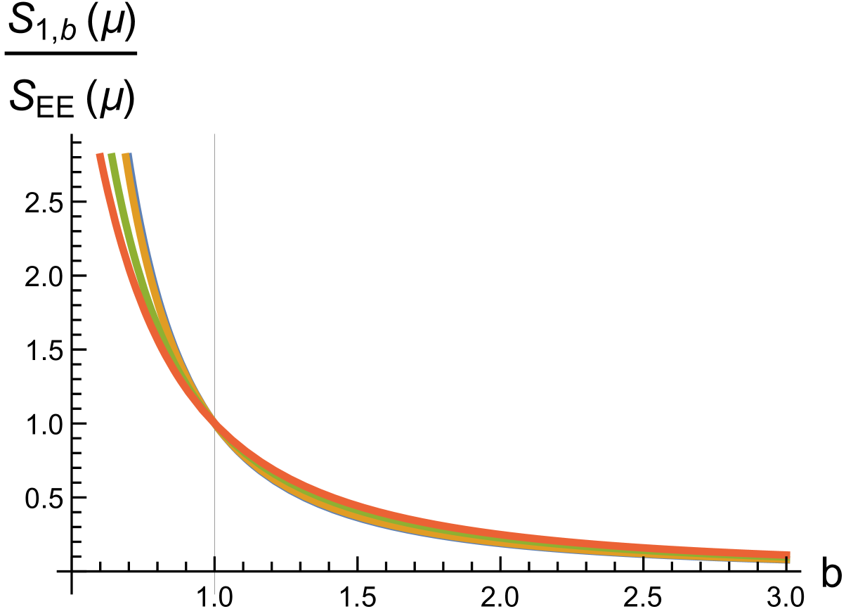
(b)

Figure 1: Plots of $S_{1,b}(\mu)/S_{EE}(\mu)$ as a function of $b$ in $d=4$ for various $\mu$. (a) Normalized by $S_{EE}(0)$; curves have $\mu=$ 0 (blue), 1 (orange), 2 (green), 3 (red). (b) Normalized by $S_{EE}(\mu)$; same values of $\mu$ except the green and red curves correspond to $\mu=5,100$, respectively. The blue and and orange curves largely overlap. We have set $\ell_{\ast}=2\pi$.

Let’s consider some more interesting limits. It is straightforward to work out

$$\lim_{q\to 0}S_{q,b}(\mu)=\frac{S_{EE}}{2}\left(\frac{2}{d}\right)^{d}\left(\frac{1}{b^{2}q}\right)^{d-1}\;.$$ (40)

and

$$\lim_{b\to 0}S_{q,b}(\mu)=\frac{S_{EE}}{2(q(d-1)x_{11}/2-(q-1))}\left(\frac{2}{d}\right)^{d}\left(\frac{1}{b^{2}q}\right)^{d-1}\;.$$ (41)

Note that the first limit is independentof $\mu$ to leading order, matching the neutral case Johnson:2018bma .

Next,

$$\lim_{q\to\infty}S_{q,b}(\mu)=\frac{S_{EE}}{2}\frac{\biggr{\{}x_{11}^{d-2}\left(1+\frac{(d-2)}{2(d-1)}\left(\frac{\mu\ell_{\ast}}{2\pi}\right)^{2}+x_{11}^{2}\right)-\left(\frac{x_{\infty}}{b}\right)^{d-2}\left(1+\frac{(d-2)}{2(d-1)}\left(\frac{\mu\ell_{\ast}}{2\pi}\right)^{2}+x_{\infty}^{2}\right)\biggr{\}}}{[1+(d-1)(b^{2}-1)x_{11}/2]}\;,$$ (42)

$$\lim_{b\to\infty}S_{q,b}(\mu)=\frac{S_{EE}}{(d-1)b^{2}}x_{11}^{d-3}\left[1+\frac{(d-2)}{2(d-1)}\left(\frac{\mu\ell_{\ast}}{2\pi}\right)^{2}+x_{11}^{2}\right]\;,$$ (43)

$$\lim_{\mu\to\infty}S_{q,b}(\mu)=\frac{2S_{EE}}{(b^{2}-1)}\sqrt{\frac{2d}{(d-1)}}\left(\frac{(d-2)^{2}}{2d(d-1)}\right)^{(d-2)/2}\left(\frac{\mu\ell_{\ast}}{2\pi}\right)^{d-1}\left(1-\frac{1}{b^{d-2}}\right)\;.$$ (44)

We observe that the $q\to\infty$ limit leads to some particular finite value, and matches $\lim_{q\to 1}S_{q}$ found in Belin:2013uta when we set $b=1$. Moreover, we see $S_{q,b}$ will vanish for large $b$, similar to the uncharged case Johnson:2018bma . A difference between $S_{q}(\mu)$ and $S_{q,b}(\mu)$ at large $\mu$ is $\lim_{\mu\to\infty}S_{q,b}(\mu)$ has $b$ dependence, though is independent of index $q$.

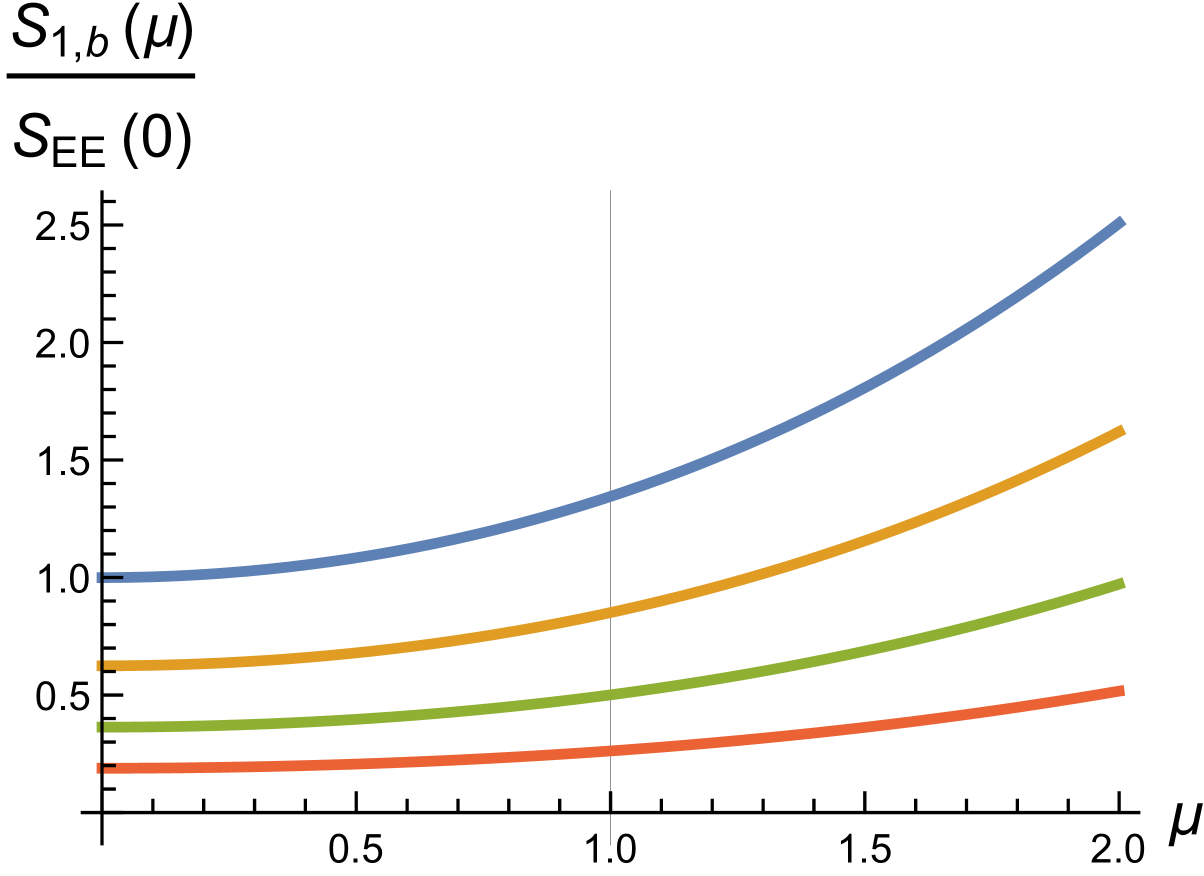
(a)

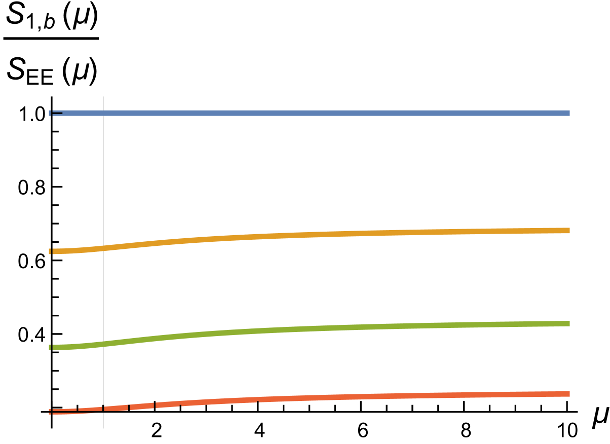
(b)

Figure 2: Plots of $S_{1,b}(\mu)/S_{EE}(\mu)$ as a function of $\mu$ in $d=4$ for various $b$. (a) Normalized by $S_{EE}(0)$; curves have $b=$ 1 (blue), 1.2 (orange), 1.5 (green), 2 (red). (b) Normalized by $S_{EE}(\mu)$. We have set $\ell_{\ast}=2\pi$.

Drastically different behavior for $S_{1,b}(\mu)$ is observed in Figure 1 and Figure 2 corresponding to the way we normalize $S_{1,b}(\mu)$. Indeed, based on our expectation that $\lim_{b\to 1}S_{1,b}(\mu)$ should approach unity, we find that we must normalize our $S_{q,b}(\mu)$ by (39), as opposed to $S_{EE}(0)$. Notice when we normalize by $S_{EE}(0)$ we see that $\mu$ has much more influence compared to when we normalize by $S_{EE}(\mu)$. In either normalization, however, the central feature evident in these figures is for $b>1$, as the index $b$ increases the entropy $S_{1,b}(\mu)$ decreases. Unlike $S_{q}(\mu)$, we see at large $b$ the entropy $S_{1,b}$ will vanish, however, the chemical potential $\mu$ can help stave off this limit, as seen by (43).

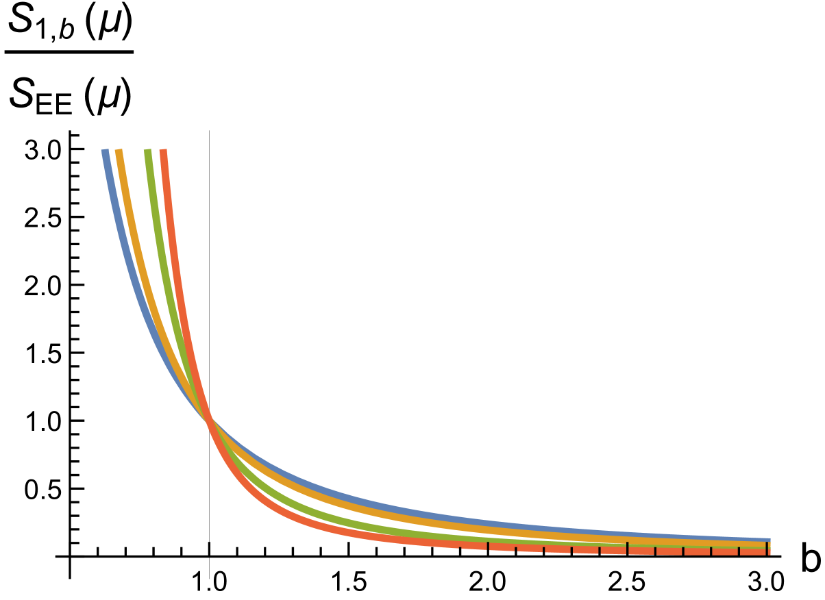
(a)

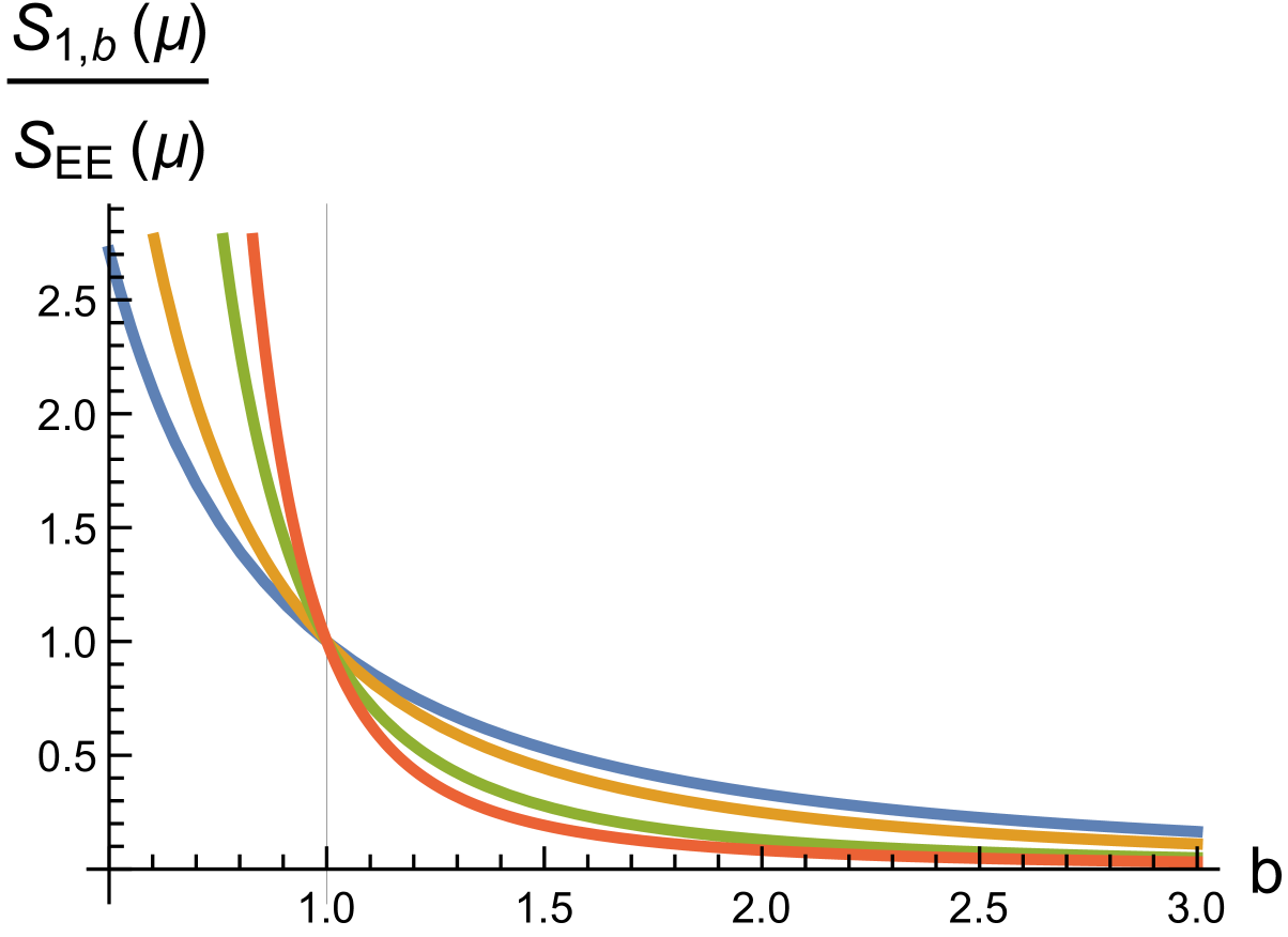
(b)

Figure 3: A plot of $S_{1,b}(\mu)/S_{EE}$ as a function of $b$ in a variety of dimensions: $d=3$ (blue), $d=4$ (orange), $d=7$ (green), and $d=10$ (red). Here we have normalized by $\lim_{b\to 1}S_{1,b}(\mu)$ and set $\ell_{\ast}=2\pi$. (a) Chemical potential $\mu=1$, (b) $\mu=100$.

In Figure 3 we plot the dimension $d$ dependence of $S_{1,b}(\mu)$. For $b>1$, we see larger $d$ leads to smaller $S_{1,b}$; for $b<1$ larger $d$ corresponds to higher $S_{1,b}(\mu)$. We also observe that, starting at $b=1$ (where we have normalized by $S_{EE}(\mu)$) all curves meet, separate and then vanish as $b$ goes large. We find the expected divergences in $S_{1,b}(\mu)$ as $b$ approaches zero, where different dimensions clearly separate out $S_{1,b}(\mu)$. Notice, moreover, the spread increases between the curves above and below $b=1$ as $\mu$ increases.

The traditional Rényi entropy is known to satisfy a number of inequalities Hung:2011nu , namely,

$$\begin{split}&\frac{\partial S_{q}}{\partial q}\leq 0\;,\quad\frac{\partial}{\partial q}\left(\frac{q-1}{q}S_{q}\right)\geq 0\;,\\ &\frac{\partial}{\partial q}[(q-1)S_{q}]\geq 0\;,\quad\frac{\partial^{2}}{\partial q^{2}}[(q-1)S_{q}]\leq 0\;.\end{split}$$ (45)

These inequalities also hold for both the neutral and charged holographic Rényi entropies Hung:2011nu ; Belin:2013uta . The reason these inequalities hold in either case is because the CFT, via the CHM map, lives on a stable thermal ensemble; the presence of a global conserved charge in the field theory does not alter the stability of the ensemble.

It is natural to ask whether the entropy $S_{1,b}(\mu)$ will satisfy a similar set of inequalities. If so, we are more inclined to refer to the object as a Rényi entropy. It is evident from Figure 1 and Figure 3 that the slope of $S_{1,b}(\mu)$ is negative, even when we are in the neutral limit $\mu=0$. In Figure 4 we numerically investigate the function $(b^{2}-1)S_{1,b}(\mu)$, which allows us to conclude our $S_{1,b}(\mu)$ satisfies a similar set of inequalities that $S_{q}(\mu)$ does:

$$\begin{split}&\frac{\partial S_{1,b}}{\partial b}\leq 0\;,\quad\frac{\partial}{\partial b}[(b^{2}-1)S_{1,b}]\geq 0\;,\quad\frac{\partial^{2}}{\partial b^{2}}[(b^{2}-1)S_{1,b}]\leq 0\;.\end{split}$$ (46)

Recall from the $(p,V)$ plane that a change in $b$ corresponds to a change pressure. Even though vertical shifts in pressure below the $M=0$ curve leads to negative mass systems, there is no thermal phase transition of the hyperbolic charged black hole. Indeed, since the thermodynamic volume $V$ scales as the entropy (26), the heat capacity at fixed volume $C_{V}=0$. It is unclear what the exact field theory interpretation of the inequalities presented in (46), though it is expected that it also follows from the fact the CFT living on the hyperbolic cylinder is in a stable thermal ensemble.

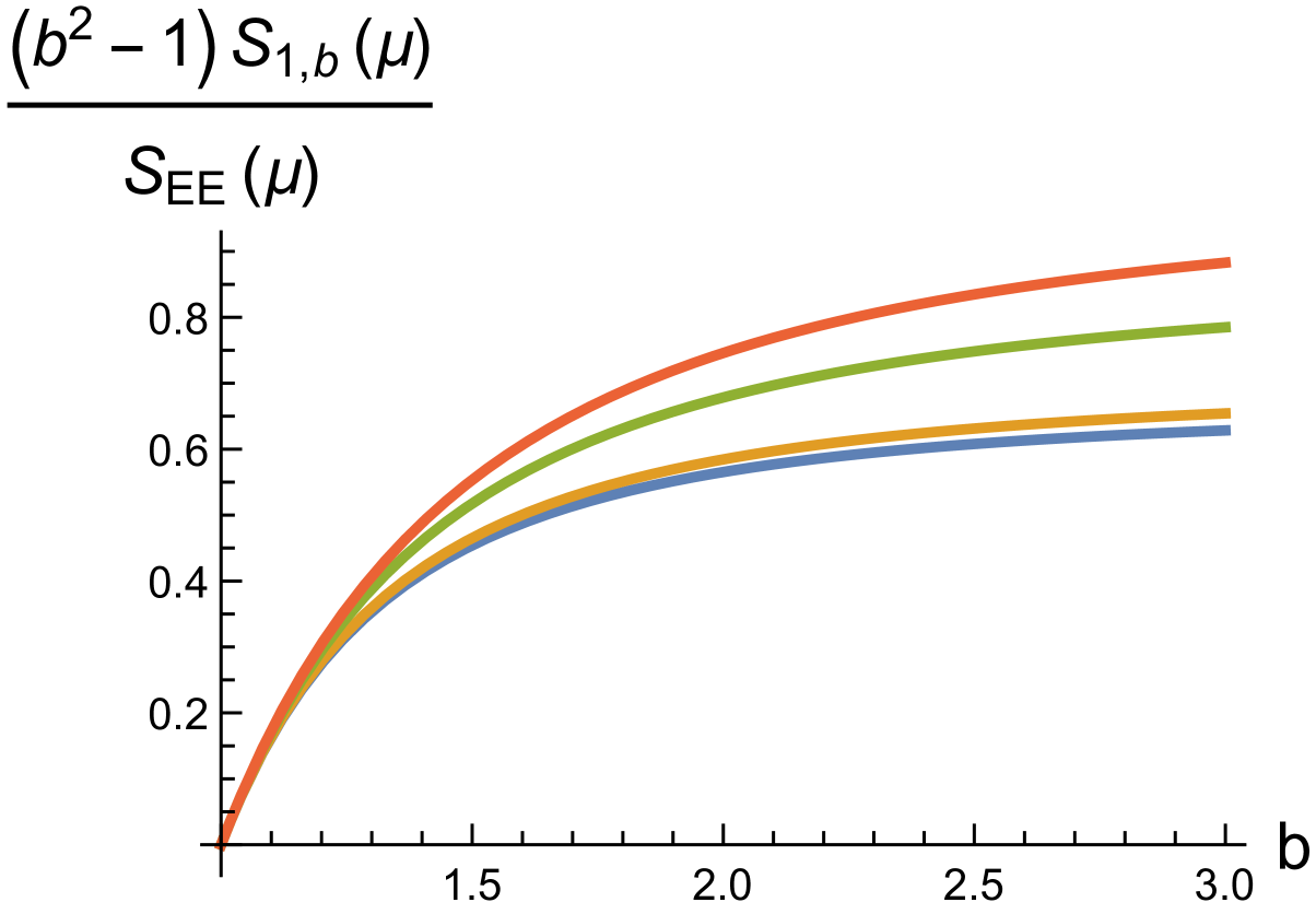
(a)

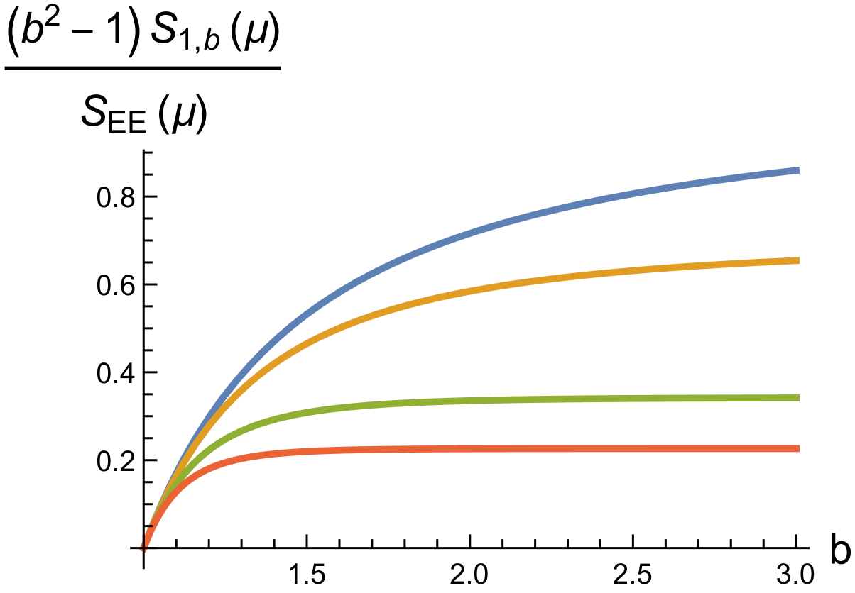
(b)

Figure 4: A plot of $(b^{2}-1)S_{1,b}(\mu)/S_{EE}$ as a function of $b$, normalized by $S^{b\to 1}_{EE}(\mu)$. (a) A variety of fixed potential $\mu$: $\mu=0$ (blue), $\mu=1$ (orange), $\mu=5$ (green), $\mu=100$ (red). (b) A variety of dimensions $d$: $d=3$ (blue), $d=4$ (orange), $d=7$ (green), and $d=10$ (red). The origin has been set at $b=1$.

3.3 Choices of $b(q)$

Thus far we have really only explored the behavior of $S_{1,b}(\mu)$ as a function of the chemical potential $\mu$. We can of course leave the usual Rényi index $q$ turned on and consider different behaviors of the new index $b$, i.e., $b$-deformations of $S_{q}(\mu)$. For example, in Figure 5 we simply fix the parameter $b=2$ and analyze how $S_{q,2}(\mu)$ changes as a function of $\mu$, $q$ and $d$. As observed, selecting $b\neq 1$ leads to divergences at the critical values of $q_{c}$ (34), the location of which depends on both $\mu$ and $d$. We see low values of $\mu$, compared to values of $d$, force the the divergence in $S_{q,2}(\mu)$ to occur for smaller values of $q$. This is because at fixed $d$ as $\mu$ increases, even for relatively low $\mu$, the $\mu^{2}$ term in $x_{11}$ becomes dominant quickly since it also couples to the dimension at order $O(d^{2})$.

We can also see how $S_{q,b}(\mu)$ changes when $b=b(q)$. In Figure 6, for example, we consider when $b=q$, for which we observe the expected concave up behavior of Rényi entropies. We also point out the slightly different influences between dimension $d$ and $\mu$, where higher $d$ lowers the (local) minimum of $S_{q,q}$ but higher $\mu$ raises the minimum.

There are two specific special cases of $b(q)$ which we study in more detail below.

Special Cases

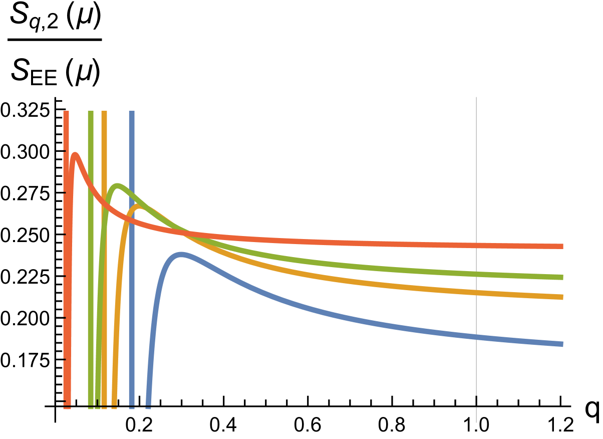
(a)

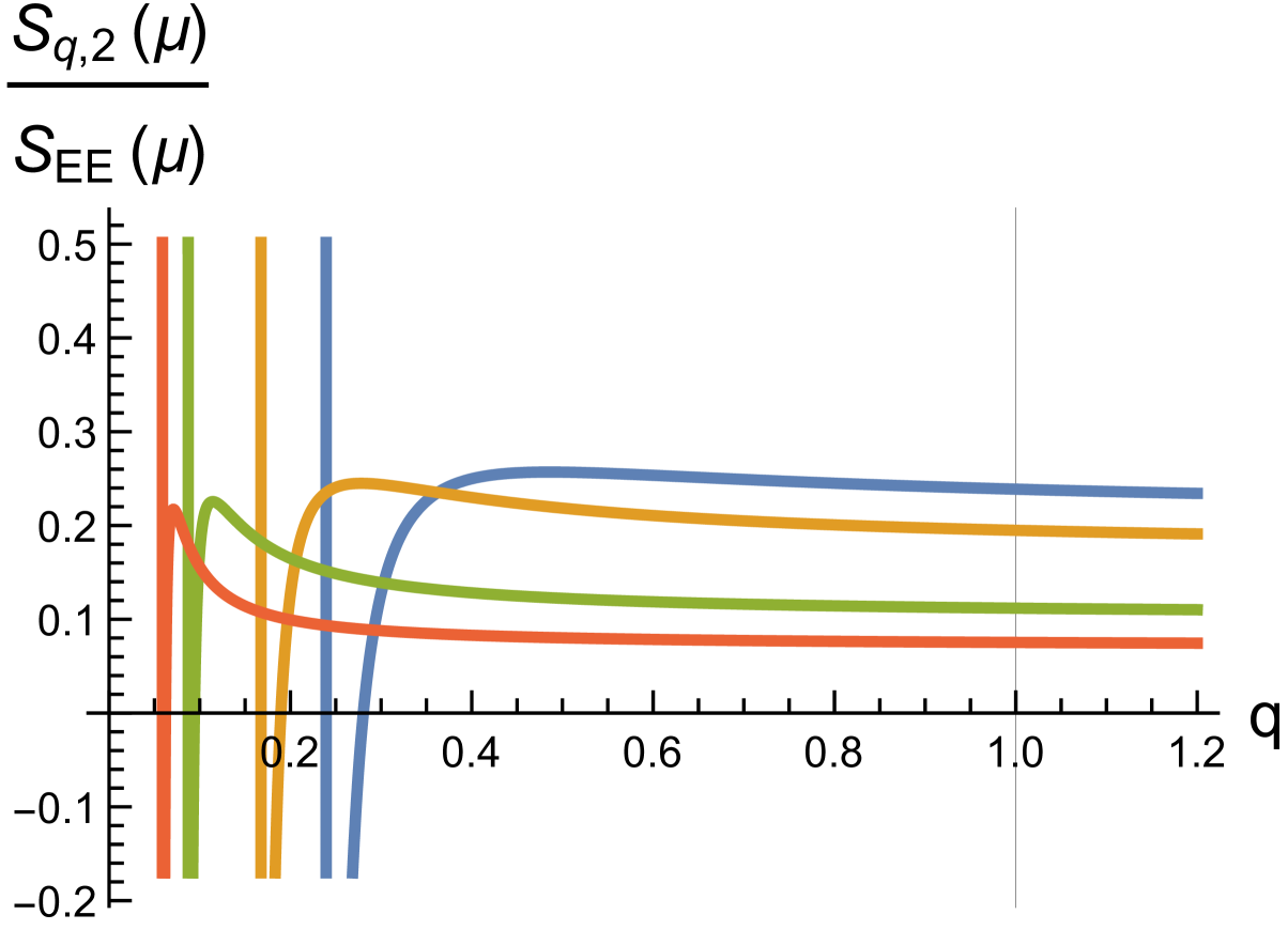
(b)

Figure 5: A plot of $S_{q,2}(\mu)$ as a function of $q$ for different $\mu$ and $d$. (a) Fixed potential $\mu$: $\mu=0$ (blue), $\mu=1$ (orange), $\mu=1.5$ (green), $\mu=2$ (red); $d=4$. (b) Dimensions $d$: $d=3$ (blue), $d=4$ (orange), $d=7$ (green), and $d=10$ (red); $\mu=1$. Notice relatively small values of $\mu$ lead to smaller values of $q_{c}$.

As first explored in Johnson:2018bma and reviewed in Section 2, for $q,b\neq 1$, there are particular choices for $b,q$ which lead to interesting insights for $S_{q,b}(\mu)$. These specific choices pertain to types of $b$-deformations which correspond to interesting changes in the $(p,V)$ plane: (i) a completely vertical displacement away from the $T_{0}/q$ isotherm to the $T_{0}$ line (the massless hyperbolic curve), i.e., no volume change. This case is interesting because it provides a special pair of values of $(q,b)$ other than $1$ such that $S_{q,b}=S_{EE}$; (ii) a change in pressure along the $T_{0}/q$ isotherm such that we land back on the $T_{0}$ curve, corresponding to the particular value $b=q^{-1}$.

In the charged scenario we can consider these special cases as well. (i) Now a completely vertical displacement straight from the $T_{0}/q$ isotherm, where $x_{qb}=\frac{r_{h}}{L}$ and $L=L_{0}/b$, to the $T_{0}$ isotherm, where $r_{h}=L_{0}x_{11}$, corresponds to when $x_{qb}=bx_{11}$. This leads to the following relation between $b$ and $q$:

$$(b^{2}-1)=\frac{2}{qdx_{11}}\left[1-\frac{q}{x_{11}}+\frac{dq}{2x_{11}}(1-x_{11})\right]+\frac{(d-2)^{2}}{2d(d-1)x_{11}}\left(\frac{\mu\ell_{\ast}}{2\pi}\right)^{2}\;.$$ (47)

Substituting this choice for $b=b(q,\mu)$ into $S_{q,b}(\mu)$ (32), we find after some algebra that

$$S_{q,b}(\mu)|_{x_{qb}=bx_{11}}=S_{EE}(\mu)\;,$$ (48)

where the charged von Neumann entropy $S_{EE}(\mu)$ is displayed in (39). Thus, as in the neutral limit, there exist special values of $b$ and $q$ not equal to 1 such that $S_{q,b}(\mu)=S_{EE}(\mu)$. From the extended black hole thermodynamics perspective this is not surprising since the constant volume paths are equivalent to constant entropy paths.

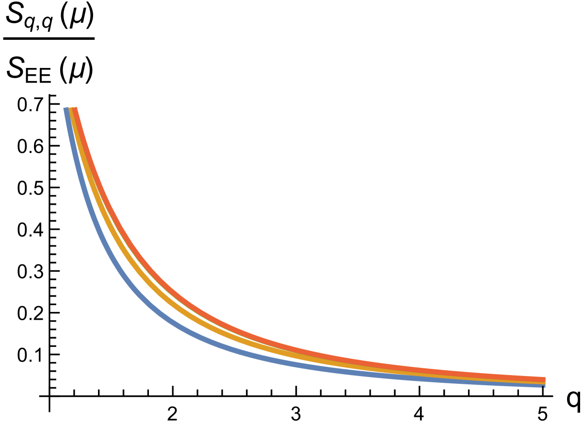
(a)

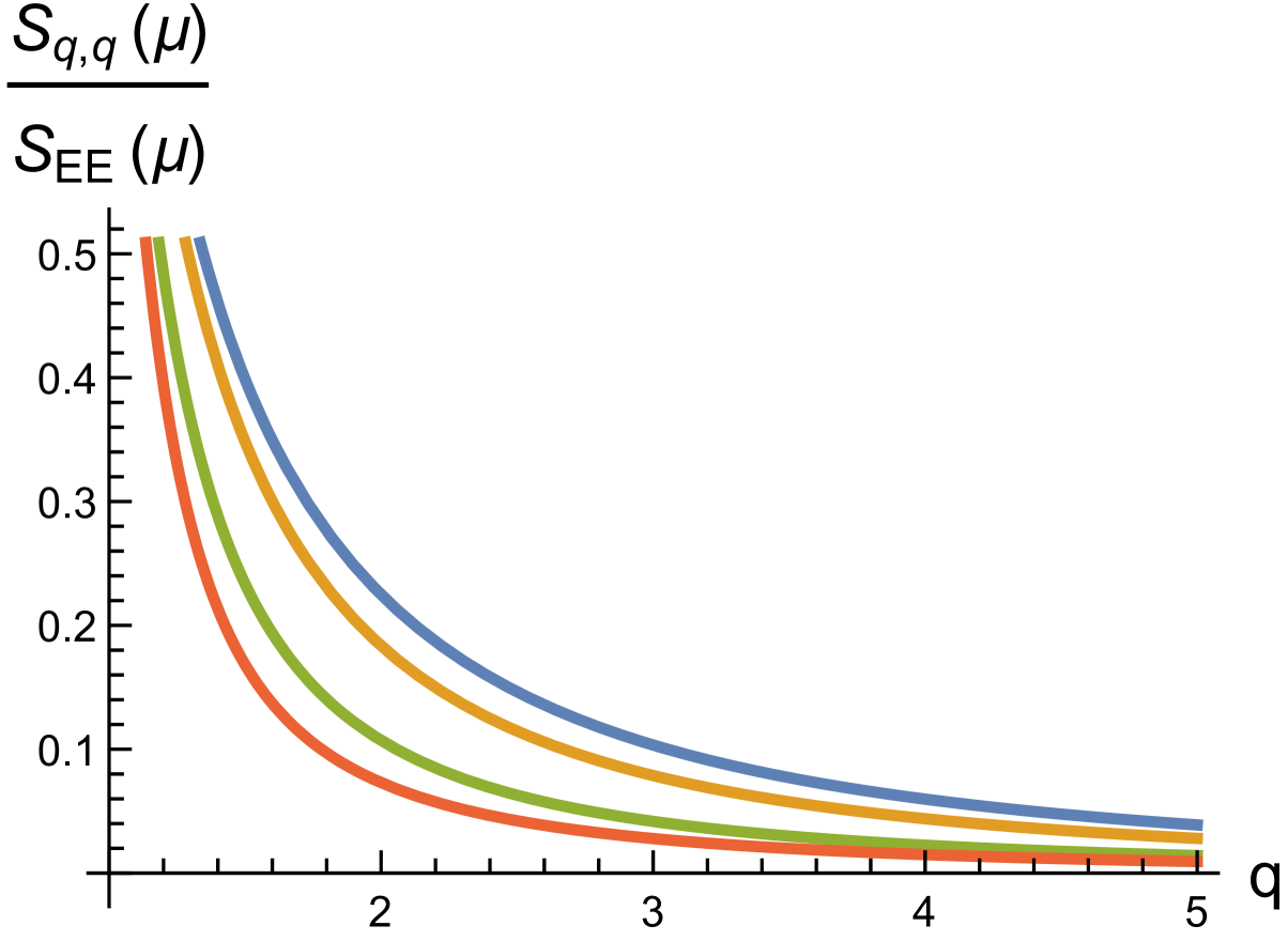
(b)

Figure 6: A plot of $S_{q,q}(\mu)$ as a function of $q$ for different $\mu$ and $d$. (a) Fixed potential $\mu$: $\mu=0$ (blue), $\mu=5$ (orange), $\mu=50$ (green), $\mu=100$ (red); $d=4$. (b) Dimensions $d$: $d=3$ (blue), $d=4$ (orange), $d=7$ (green), and $d=10$ (red); $\mu=1$.

(ii) A change in pressure along the $T_{0}/q$ isotherm such that we return to the $T_{0}$ isotherm we have $x_{qb}=x_{11}$. This results in the following relation between $b,q$ and $\mu$:

$$b=q^{-1}\frac{2x_{11}}{dx_{11}^{2}-(d-2)+\frac{(d-2)^{2}}{2(d-1)}\left(\frac{\mu\ell_{\ast}}{2\pi}\right)^{2}}\;.$$ (49)

Observe that in the neutral limit we recover the special case $b=q^{-1}$. Substituting (49) into $S_{q,b}(\mu)$ leads to a cumbersome relation which we won’t express here. Importantly, from Figure 7 and Figure 8 we see that as $q$ grows the $S_{q,b(q)}(\mu)$ grows quickly as $\mu$ or the dimension $d$ increase. This is similar to what is observed in the neutral case Johnson:2018bma . In the neutral case, moreover, it was argued that the index $b$ can be thought of as a parameter which undoes the replica trick of creating $q$-copies of $\rho_{R}$ on flat space, hence the $b=q^{-1}$. This was explicitly verified in the $d=2$ case Johnson:2018bma . Since the charged Rényi entropy can likewise be computed using the replica trick, it is also natural to interpret $b=q^{-1}$. We found, motivated by extended thermodynamics that we have $b\propto q^{-1}$, where the proportionality constant explicitly depends on the potential $\mu$. For purposes of comparison, in Figure 7 and Figure 8 we have included plots of $S_{q,q^{-1}}(\mu)$, in which we observe similar qualitative features, however, the influence of $\mu$ and $d$ are enhanced when we choose (49). We of course point out a crucial difference on the dependence in $\mu$ in Figure 7: When $b$ is given by (49), larger values of $\mu$ correspond to large values of $S_{q,b}$, the opposite of what is seen when $b=q^{-1}$.

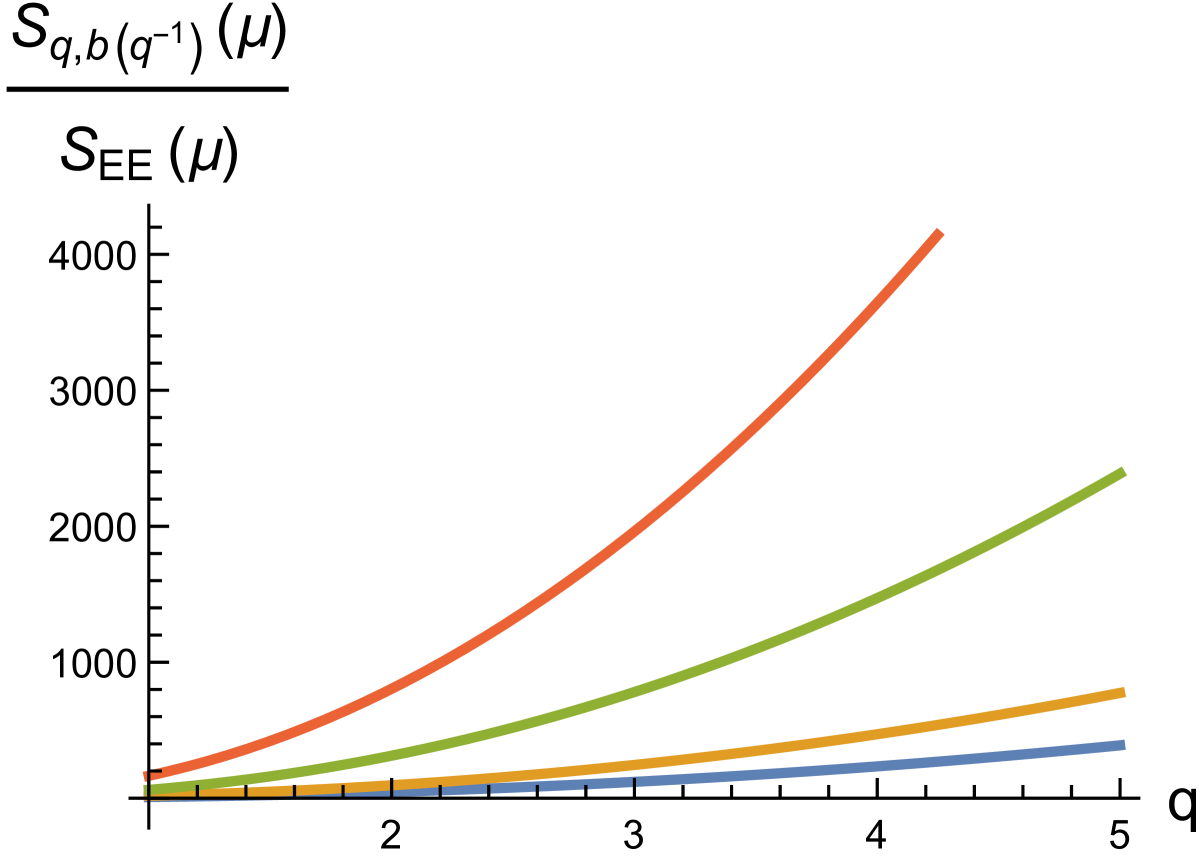
(a)

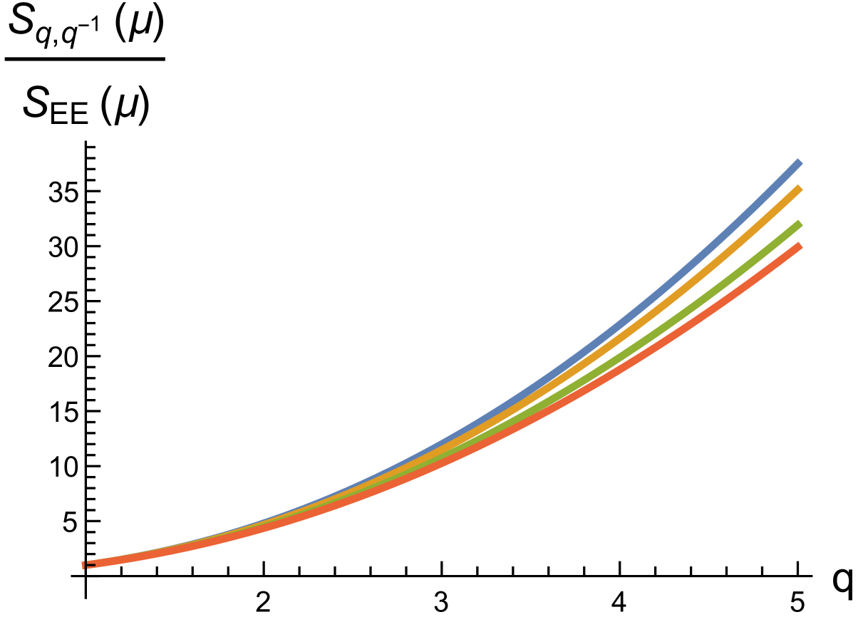
(b)

Figure 7: A plot of $S_{q,b(q^{-1})}(\mu)$ as a function of $q$ for different $\mu$. (a) $b\propto q^{-1}$ (49). (b) $b=q^{-1}$. In both (a) and (b) $d=4$ and $\mu=0$ (blue), $\mu=1$ (orange), $\mu=2$ (green), $\mu=3$ (red).

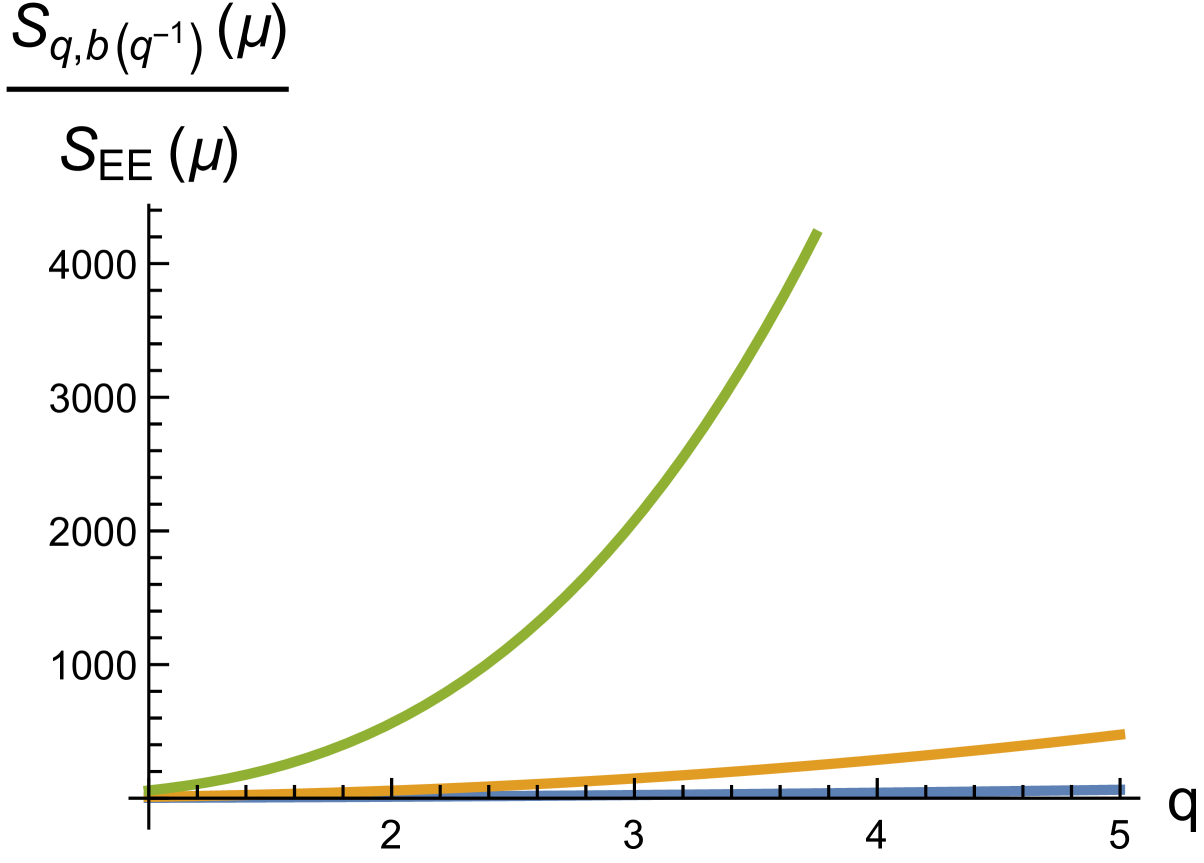
(a)

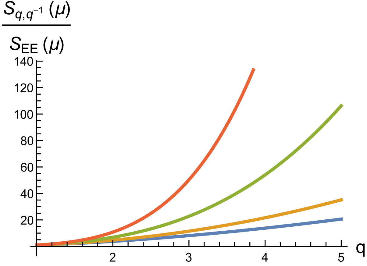
(b)

Figure 8: A plot of $S_{q,b(q^{-1})}(\mu)$ as a function of $q$ for different $d$. (a) $b\propto q^{-1}$ (49) with $\mu=.5$. (b) $b=q^{-1}$ with $\mu=1$. In both cases $d=3$ (blue), $d=4$ (orange), and $d=5$ (green); in (b) we also have $d=6$ (red).

Imaginary Chemical Potential

In field theory, both real and imaginary $\mu$ are of interest. As in the non-extended case Belin:2013uta we can simply analytically continue our above holographic calculations by setting

$$\mu\to i\mu_{E}\Rightarrow q_{e}\to iq^{E}_{e}\;,$$ (50)

where $\mu_{E}$ and $q^{E}_{e}$ are purely real. Therefore, an imaginary chemical potential is dual to an imaginary charge. The consequences of this continuation is that the root $x_{qb}$ (33) will fail to exist when $\mu_{E}$ becomes too large. Specifically,

$$\mu_{E}\leq\frac{2(d-1)}{(d-2)}\left(\frac{2\pi}{\ell_{\ast}}\right)^{2}\left(1+\frac{1}{q^{2}b^{2}d(d-2)}\right)\;.$$ (51)

At fixed $q$, for $\mu_{E}$ larger than this upper bound, the event horizon will disappear leaving a naked singularity.

In Figures 9 and 10 we explore the behavior of $S_{q,b}(\mu_{E})$. Comparing Figure 9 to Figure 2, we see that $S_{1,b}(\mu_{E})$ will increase, rather than decrease, for increasing $\mu_{E}$; similar behavior is seen in the $S_{q,1}(\mu_{E})$ case when normalized by $S_{EE}(0)$ Belin:2013uta , however, we find no decrease in $S_{1,b}(\mu_{E})/S_{EE}(\mu_{E})$ as $\mu_{E}$ increases. Note, moreover, from Figure 9 (b) we see for $b<1$ the entropy increases as $\mu_{E}$ increases. In Figure 10, where we study $S_{q,2}(\mu_{E})$, we find an interesting difference between the choice of normalization. When we normalized by $S_{EE}(0)$ the entropy $S_{q,2}(\mu_{E})$ will monotonically decrease as $\mu_{E}$ increases, while normalized by $S_{EE}(\mu_{E})$ the entropy will increase before approaching a local maximum.

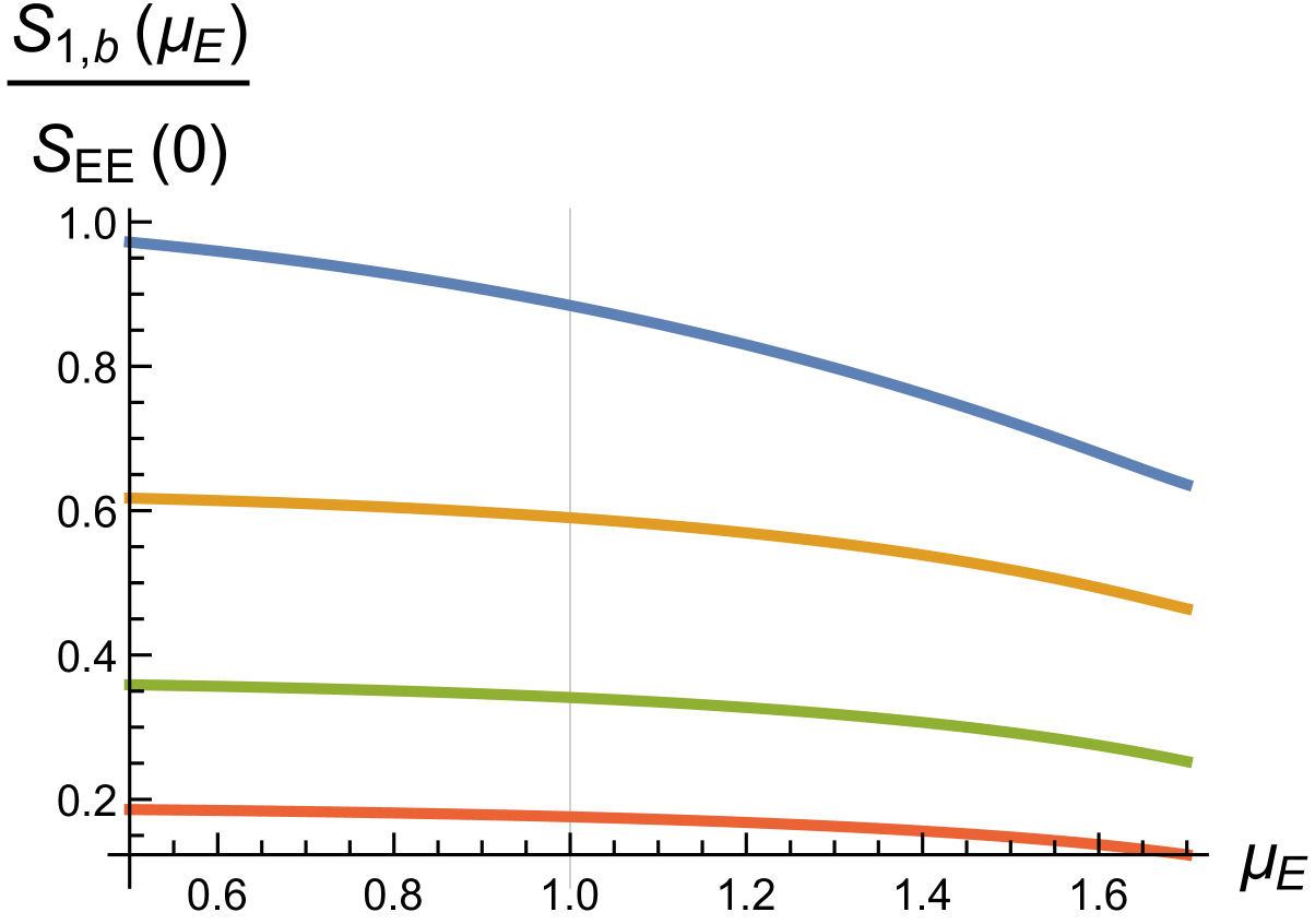
(a)

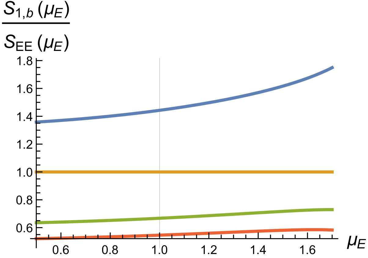
(b)

Figure 9: A plot of $S_{1,b}(\mu_{E})$ as a function of $\mu_{E}$ for different $b$. (a) Normalized by $S_{EE}(0)$ with $b=1$ (blue), $b=1.2$ (orange), $b=1.5$ (green) and $b=2$ (red). (b) Normalized by $S_{EE}(\mu_{E})$ with $b=.9$ (blue), $b=1$ (orange), $b=1.2$ (green) and $b=1.3$ (red). Here we have set $d=4$.

4 Field Theory Interpretation

Our generalized charged Rényi entropy (32) was physically well motivated by the extended thermodynamics of charged AdS black holes. It is worthwhile to think about the field theory interpretation of $S_{q,b}(\mu)$, and how it would be constructed on the field theory side. This can be accomplished, at least in principle, by working backwards from our expression (32) whereby we identify the proper generalization of the CHM map (4).

More precisely, to connect the flat space CFT state $\rho_{A}^{(b)}$ to the thermal ensemble on $\mathbb{R}\times\mathbb{H}^{d-1}$, given by $\rho_{therm}$, we would introduce the density matrix $\rho_{A}^{(b)}$ of the following form:

$$\rho_{A}^{(b)}(\mu)=U^{\dagger}\left(\frac{e^{-H/T_{0}+b^{2}p_{0}V_{0}/T_{0}+\mu Q_{A}}}{Z(T_{0},p_{0},\mu)}\right)U\;.$$ (52)

The matrix in between the unitaries $U^{\dagger}$ and $U$ is the extended version of the thermal ensemble density matrix $\rho_{therm}$ used in the CHM map, and the thermal partition function formally given by $\text{tr}[\exp(-H/T_{0}+b^{2}p_{0}V_{0}/T_{0}+\mu Q_{A})]$.

The charged generalization of the entropy $S_{q,b}(\mu)$ is then

$$S_{q,b}(\mu)=\frac{1}{[(1-q)-q(d-1)x_{11}(b^{2}-1)/2]}\log\left[\text{tr}(\rho^{(b)}_{A})^{q}\right]\;,$$ (53)

which came from us writing $S_{q,b}(\mu)$ as a difference of logarithms of two partition functions Johnson:2018bma

$$S_{q,b}=\left[1+qx_{11}\left(\frac{d-1}{2}\right)\left(\frac{b^{2}-1}{q-1}\right)\right]^{-1}\frac{1}{1-q}\log\left[\frac{Z(T_{0}/q,\mu,b^{2}p_{0})}{Z(T_{0},\mu,p_{0})^{q}}\right]\;.$$ (54)

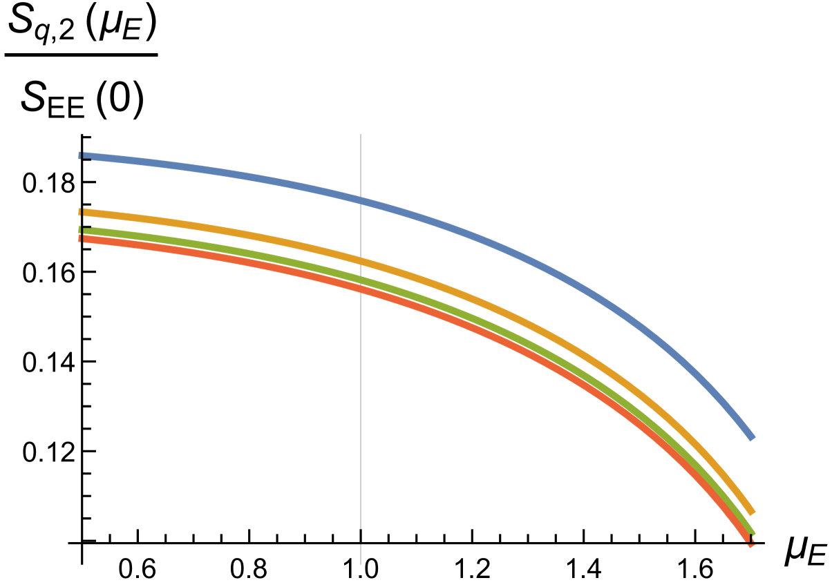
(a)

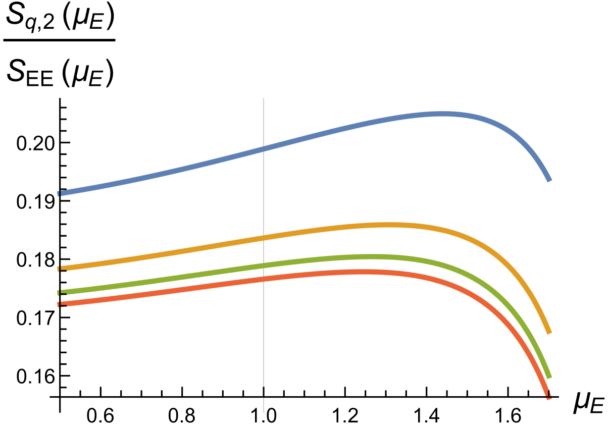
(b)

Figure 10: A plot of $S_{q,2}(\mu_{E})$ as a function of $\mu_{E}$ for different $q$. (a) Normalized by $S_{EE}(0)$. (b) Normalized by $S_{EE}(\mu_{E})$. Here we have set $d=4$ and selected $q=1$ (blue), $q=2$ (orange), $q=3$ (green) and $q=4$ (red).

The interpretation of $\rho_{A}^{(b)}$ is simply the charged generalization of $\rho_{A}^{(b)}(0)$, first given in Johnson:2018bma : It is the $b$th power of some other density matrix, denoted by $\rho_{B}$, arising from fractionating the system $A$ into $b$ copies each of length $L_{0}/b$. We then presume to glue each of the $b$ copies together, creating a system of length $L_{0}$, such that

$$\rho_{A}^{(b)}=\rho_{B}^{b}\;\;.$$ (55)

Notice the chemical potential $\mu$ simply goes along for the ride, supplementing the CHM map by inserting a Wilson line along the Euclidean time circle into the thermal path integral for $Z(T_{0}/q,\mu,b^{2}p_{0})$.

Thus, the integer $b$ has a natural interpretation as another type of Rényi index, similar to the role of $q$, at least from the perspective of the replica trick. Moreover, while it is unclear what precisely $\rho_{B}$ is measuring, the state (55) informs us of a potentially special value for $b$, namely, $b=1/q$, such that the $q$th replica of the sector at temperature $T_{0}/q$ is cancelled by the $1/q$th replica of the sector at pressure $q^{2}p_{0}$. When $\mu=0$, it was shown in Johnson:2018bma this interpretation holds precisely for the $d=2$ case, where an explicit CFT calculation involving twist operators reveals that $b=1/q$ undoes the $q$th replica in the temperature sector. It behooves us then to study the $d=2$ case, where it is possible to carry out a precise CFT calculation using charged twist operators Belin:2013uta . However, we do not yet have the corresponding $d=2$ holographic computations completed since this requires us to consider the geometry of a $2+1$-dimensional charged AdS black hole, for which the geometry changes dramatically Martinez:1999qi . We will study these holographic calculations in the next section.

Fortunately, we can make some progress in understanding the interpretation of $b$ for $d>2$ by generalizing the conformal dimensions of the higher dimensional twist operators.

4.1 Twist Operators in Higher Dimensions

Just like its uncharged counterpart, the calculation of charged Renyí entropies can be achieved by inserting a twist operator $\sigma_{q}$ at the entangling surface. The twist operators have an associated conformal dimension $h_{q}$ which appears in correlation functions of the twist operators. In the charged case, the conformal dimension of the twist operators is generalized by considering the leading singularity in the correlator $\langle T_{\mu\nu}^{CFT}\sigma_{q}\rangle$. The leading singularity takes the form Belin:2013uta , for example, tangentially along the entangling surface,

$$\langle T^{CFT}_{ab}\sigma_{q}\rangle=-\frac{h_{q}}{2\pi}\frac{1}{y^{d}}\delta_{ab}\;.$$ (56)

Here $y$ is the perpendicular distance from $\sigma_{q}$ such that $y$ is much smaller than any scales defining the geometry of the entangling surface, $T_{ab}^{CFT}$ is the CFT energy-momentum tensor along the tangential directions $a,b$ to $\sigma_{q}$, and $h_{q}$ is a constant representing the conformal dimension of $\sigma_{q}$. Generically $h_{q}$ is given in terms of the thermal energy density $\mathcal{E}(T,\mu)$ on the hyperbolic cylinder Hung:2011nu ,

$$h_{q}(\mu)=\frac{2\pi qL_{0}^{d}}{(d-1)}[\mathcal{E}(T_{0},\mu=0)-\mathcal{E}(T_{0}/q,\mu)]\;.$$ (57)

These conformal dimensions can be computed holographically using the energy densities $\mathcal{E}$ of the boundary field theory, which is proportional to the mass $M$ of the dual hyperbolic black hole Belin:2013uta

$$h_{q}=\frac{2\pi qL_{0}^{d}}{(d-1)}[\mathcal{E}(T_{0},\mu=0)-\mathcal{E}(T_{0}/q,\mu)]=\frac{2\pi q}{w_{d-1}}\frac{L_{0}}{(d-1)}\left[M(T_{0},\mu=0)-M(T_{0}/q,\mu)\right]\;.$$ (58)

Following the spirit of Johnson:2018bma , we can likewise obtain the conformal weights $h^{(b)}_{q}$ for the twist operators $\sigma_{q}^{(b)}$ just by using the extended thermodynamics of the charged black hole

$$h_{q}^{(b)}=\frac{2\pi q}{w_{d-1}}\frac{L_{0}}{(d-1)}\left[M(T_{0},p_{0},\mu=0)-M(T_{0}/q,b^{2}p_{0},\mu)\right]\;.$$ (59)

Since $M$ is interpreted as the enthalpy in extended black hole thermodynamics, we see $h_{q}^{(b)}$ is given as the difference of a state function.

Evaluating our expression for the mass $M(x,L,\mu)$ (23), we have that $M(T_{0},p_{0},\mu=0)=0$, as this corresponds to a massless hyperbolic black hole, and at $M(T_{0}/q,L_{0}/b,\mu)$, where $x=x_{qb}$. Therefore,

$$h_{q}^{(b)}(\mu)=\frac{qL_{0}^{d-1}}{8G_{N}}\left[\left(\frac{x_{qb}}{b}\right)^{d-2}(1-x_{qb}^{2})-\left(\frac{x_{qb}}{b}\right)^{d-2}\frac{(d-2)}{2(d-1)}\left(\frac{\mu\ell_{\ast}}{2\pi}\right)^{2}\right]\;.$$ (60)

This is interpreted as the $b$-deformation of the conformal weight of the $d$-dimensional twist operators $\sigma_{q}$ first explored in Hung:2014npa .

Two remarks are in order: (1) Special values of $h_{q}^{(b)}(\mu)$, and (2) Derivatives of $h_{q}^{(b)}(\mu)$.

Special Values of $h_{q}^{(b)}(\mu)$

Let’s first consider the behavior of $h_{q}^{(b)}$ when $\mu=0$ for some particular special values of $q,b$. Consider when $x_{qb}=b$, such that $b^{2}-1=2(1-q)/qd$. This choice for $b$, recall, corresponds to the special value when $S_{q,b\neq 1}=S_{EE}$. The corresponding conformal weight is

$$h^{(b)}_{q}=\frac{qL_{0}^{d-1}}{8G_{N}}(1-b^{2})=\frac{L_{0}^{d-1}}{4G_{N}}\frac{(q-1)}{d}\;.$$ (61)

Since this choice of $b(q)$ has $S_{q,b(q)}$ equal to the von Neumann entropy $S_{EE}$, we recognize there exists a replica trick to compute $\text{tr}[(\rho^{(b)}_{A})^{q}]$ involving twist operators with a conformal weight given above will lead to a direct calculation of $S_{EE}$. Indeed, we recover the $d=2$ CFT calculation presented in Johnson:2018bma , where

$$h^{(b)}_{q}=\frac{c}{12}q\left(1-\frac{1}{q^{2}b^{2}}\right)\;,$$ (62)

upon identifying the 2-dimensional central charge $c=3L_{0}/2G_{N}$.

From (62) it is also easy to see that when $b=1/q$, i.e., $b$ ‘undoes’ the $q$-replicas, we have $h^{(b)}_{q}=0$. Holographically this corresponds to $x_{qb}=1$. Note, moreover, from (60) at $\mu=0$ we have $h^{(b=q^{-1})}_{q}=0$ for all dimensions, where $S_{q,q^{-1}}|_{d>2}\neq 0$, while the CFT calculation corresponds only to $d=2$, where $S_{q,q^{-1}}|_{d=2}=0$.

Let’s now turn the charge $\mu$ on. There are a number of potentially interesting values of $h^{(b)}_{q}(\mu)$ given a specific $(q,b)$. First note that $h^{(b)}_{q}(\mu)=0$ when

$$x_{qb}=x_{qb}^{\ast}\equiv\sqrt{\frac{d}{d-2}}x_{\infty}\;,$$ (63)

with $x_{\infty}$ defined in (36). Therefore, as we fractionate the system into a large number of $q$- or $b$-copies, the conformal weight of the twist operators will vanish; this is contrary to what we see in the neutral case, where $h^{(b)}_{q}=0$ also when $x_{qb}=1$.

Next, consider when $x_{qb}=b$, such that

$$b^{2}-1=\frac{2}{qd}(1-q)+\frac{(d-2)}{2d(d-1)}\left(\frac{\mu\ell_{\ast}}{2\pi}\right)^{2}\;.$$ (64)

Then we have

$$\begin{split}h^{(b)}_{q}(\mu)&=\frac{qL_{0}^{d-1}}{8G_{N}}\left[\frac{2}{qd}(q-1)-\frac{(d-2)(d+1)}{2d(d-1)}\left(\frac{\mu\ell_{\ast}}{2\pi}\right)^{2}\right]\;.\end{split}$$ (65)

Thus, $h^{(b)}_{q}(\mu)$ will be positive when $(q-1)>q\frac{(d-2)(d+1)}{4(d-1)}\left(\frac{\mu\ell_{\ast}}{2\pi}\right)^{2}$. Meanwhile, for $x_{qb}=1$, where

$$b=\frac{2q^{-1}}{\left(2-\frac{(d-2)^{2}}{2(d-1)}\left(\frac{\mu\ell_{\ast}}{2\pi}\right)^{2}\right)}\;,$$ (66)

we have $h^{(b)}_{q}(\mu)<0$. Specifically

$$h^{(b)}_{q}(\mu)=-\frac{qL_{0}^{d-1}}{8G_{N}b^{d-2}}\frac{(d-2)}{2(d-1)}\left(\frac{\mu\ell_{\ast}}{2\pi}\right)^{2}\;.$$ (67)

We see for this choice of $b(q)$, $h^{(b)}_{q}(\mu)$ will be negative, though $S_{q,b}$ will be positive.

There are two more particularly interesting cases to consider: (i) the special value of $b$ given in (49), corresponding to when $x_{qb}=x_{11}$, where $b\propto q^{-1}$, and (ii) when $x_{qb}=bx_{11}$. The first of these leads to

$$h^{(b)}_{q}(\mu)=\frac{qL_{0}^{d-1}}{8G_{N}}\left(\frac{x_{11}}{b}\right)^{d-2}\left[(1-x_{11}^{2})-\frac{(d-2)}{2(d-1)}\left(\frac{\mu\ell_{\ast}}{2\pi}\right)^{2}\right]\;.$$ (68)

Unlike the neutral case, for generic $d$ this is non-vanishing, demonstrating index $b$ in the charged framework does not purely undo the $q$-copies in the replica trick.

Meanwhile, when $x_{qb}=bx_{11}$, in which $S_{q,b}(\mu)=S_{EE}(\mu)$, we find

$$h^{(b)}_{q}(\mu)=\frac{qL_{0}^{d-1}}{8G_{N}}x_{11}^{d-2}\left[(1-b^{2}x_{11}^{2})-\frac{(d-2)}{2(d-1)}\left(\frac{\mu\ell_{\ast}}{2\pi}\right)^{2}\right]\;.$$ (69)

This is the charged analog of (61) which gives us the conformal dimension for the twist operator $\sigma_{q}$ necessary when computing $S_{EE}(\mu)$ using the replica trick.

Derivatives of $h_{q}^{(b)}(\mu)$

In the neutral, non-extended case, there is a universal property for the conformal weight $h_{q}$ involving its first $q$th derivative Hung:2011nu ; Hung:2014npa

$$\partial_{q}h_{q}|_{q=1}=\frac{2}{(d-1)}\pi^{1-\frac{d}{2}}\Gamma(d/2)a^{\ast}_{d}\;,$$ (70)

where $a^{\ast}_{d}$ is the central charge (22) defined by the two point function of the CFT stress energy tensor. As noted in Belin:2013uta , this universal behvavior does not readily extend to the conformal weight for the charged twist operators $\sigma_{q}(\mu)$. Rather, it is natural to study $h_{q}(\mu)$ expanded about $q=1$ and $\mu=0$,

$$h_{q}(\mu)=\sum_{a,c}\frac{1}{a!c!}h_{ac}(q-1)^{a}\mu^{c}\;,\quad h_{ab}=(\partial_{q})^{a}(\partial_{\mu})^{c}h_{q}(\mu)|_{q=1,\mu=0}\;,$$ (71)

where in particular $h_{10}|_{q=1,\mu=0}\propto a^{\ast}_{d}$. Using the holographically computed $h_{q}(\mu)$, one observes $a^{\ast}_{d}$ is precisely given by (22).

Similarly, while not considered in Johnson:2018bma we can study derivatives of $h_{q}^{(b)}$, where we expand $h_{q}^{(b)}$ about $q=1$ and $b=1$:

$$h^{(b)}_{q}=\sum_{a,c}\frac{1}{a!c!}h^{(b)}_{ac}(q-1)^{a}(b-1)^{c}\;,\quad h^{(b)}_{ac}=(\partial_{q})^{a}(\partial_{b})^{c}h_{q}^{(b)}|_{q=1,b=1}\;.$$ (72)

Obviously, $h_{10}^{(b)}=\partial_{q}h_{q}^{(b=1)}|_{q=1}\propto a^{\ast}_{d}$, namely,

$$\partial_{q}h_{q}^{(1)}=\frac{L_{0}^{d-1}}{4G_{N}}\frac{1}{(d-1)}\;,$$ (73)

with $a^{\ast}_{d}$ as in (22). With our $b$-deformation, moreover, it is natural to compute $h_{01}^{(b)}$ holographically

$$h_{01}^{(b)}=\partial_{b}h^{(b)}_{1}|_{b=1}=-\frac{L_{0}^{d-1}}{8G_{N}}2x_{1b}\frac{\partial x_{1b}}{\partial b}\biggr{|}_{b=1}=\frac{L_{0}^{d-1}}{4G_{N}}\frac{1}{(d-1)}=h_{10}^{(b)}\;.$$ (74)

This tells us that the first $b$-derivative of the generalized conformal weight $h_{q}^{(b)}$ likewise gives the central charge $a_{d}^{\ast}$.

Motivated by (71), it is straightforward to generalize (72) by including a charge $\mu$,

$$h^{(b)}_{q}(\mu)=\sum_{i,j,k}\frac{1}{i!j!k!}h^{(b)}_{ijk}(\mu)(q-1)^{i}(b-1)^{j}\mu^{k}\;,\quad h_{ijk}^{(b)}=(\partial_{q})^{i}(\partial_{b})^{j}(\partial_{\mu})^{k}h_{q}^{(b)}(\mu)\biggr{|}_{q,b=1,\mu=0}\;.$$ (75)

It is simple to show

$$\begin{split}&h_{100}^{(b)}=h_{010}^{(b)}=\frac{L_{0}^{d-1}}{4G_{N}}\frac{1}{(d-1)}\;,\quad h^{(b)}_{001}=0\;,\quad h^{(b)}_{002}=-\frac{(d-2)(2d-3)}{\pi(d-1)^{2}}\frac{\ell_{\ast}^{2}L_{0}^{d-1}}{16\pi G_{N}}\;.\end{split}$$ (76)

We don’t find additional universal features for higher derivatives of the conformal weight. It may be interesting to see how these derivatives of the conformal weight match to the would be CFT calculation.

5 Extended Charged Rényi Entropy in $d=2$

5.1 Thermodynamics of Charged BTZ Black Hole

Above we extended the charged Rényi entropy for CFTs dual to Einstein-Maxwell gravity in $d>2$. The restriction on the dimension $d$ was taken into account because it is well known the geometry of charged AdS black holes in $d=2$ is markedly different from their higher dimensional counterparts. Specifically, in $d=2$ the black hole geometry is that of a charged BTZ black hole Martinez:1999qi

$$ds^{2}=-f(r)dt^{2}+f^{-1}(r)dr^{2}+r^{2}d\theta^{2}\;,\quad f(r)=\frac{r^{2}}{L^{2}}-2m-\frac{q_{e}^{2}}{2}\log\left(\frac{r}{L}\right)\;.$$ (77)

The horizon radius $r_{h}$ is located at $f(r_{h})=0$. We observe that the geometry is not asymptotically AdS because of the logarithmic term appearing in $f(r)$. The gauge potential is given by

$$A=\frac{q_{e}}{\ell_{\ast}}\log\left(\frac{r}{L}\right)dt\;.$$ (78)

The extended thermodynamics of the charged BTZ black hole was worked out in Frassino:2015oca :

$$\begin{split}&M=\frac{4pS^{2}}{\pi}-\frac{q_{e}^{2}}{32}\log\left(\frac{32pS^{2}}{\pi}\right)\;,\quad S=\frac{\pi r_{h}}{2}\;,\quad p=\frac{1}{8\pi L^{2}}\;,\quad T=\frac{8pS}{\pi}-\frac{q_{e}^{2}}{16S}\;,\\ &\Phi_{e}\equiv\left(\frac{\partial M}{\partial q_{e}}\right)_{S,p}=-\frac{q_{e}}{16}\log\left(\frac{32pS^{2}}{\pi}\right)\;,\quad V\equiv\left(\frac{\partial M}{\partial p}\right)_{S,q_{e}}=\frac{4S^{2}}{\pi}-\frac{q_{e}^{2}}{32p}\;,\end{split}$$ (79)

where $pS^{2}=\frac{\pi x^{2}}{32}$, with $x\equiv r_{h}/L$ as usual. We emphasize that, unlike their $d>2$ counterparts, the thermodynamic volume $V$ no longer scales as the entropy $S$, i.e., the thermodynamic volume is not equivalent to the naive geometric volume. The implications of this observation will be discussed further momentarily.

It is straightforward to work out the internal energy and Gibbs free energy of the charged BTZ system:

$$U=M-pV=\frac{q_{e}^{2}}{32}\left[1-\log\left(\frac{32pS^{2}}{\pi}\right)\right]\;,$$ (80)

$$\begin{split}G&=M-TS-\Phi_{e}q_{e}=-\frac{4pS^{2}}{\pi}+\frac{q_{e}^{2}}{32}\left[2+\log\left(\frac{32pS^{2}}{\pi}\right)\right]\\ &=-\frac{x^{2}}{8}+\frac{q_{e}^{2}}{32}\left[2+\log(x^{2})\right]\;.\end{split}$$ (81)

Notice that demanding the temperature $T$ be positive (equivalently the $V\geq 0$) results in the condition

$$q_{e}^{2}\leq 4\eta\;,$$ (82)

where $\eta\equiv 32pS^{2}/\pi=x^{2}$. The parameter $\eta$ also appears in $U$, which shows that for $U>0$ implies $\eta\leq 1$ resulting in a bound on $q_{e}$ Johnson:2019wcq :

$$q_{e}^{2}\leq 4\;.$$ (83)

It is well known that the asymptotic symmetry group of a rotating (uncharged) BTZ black hole yields two copies of a Virasoro algebra; this is the famous result by Brown and Henneaux stating that quantum gravity in three dimensions is dual to a two dimensional CFT with left and right central charges $c_{L}=c_{R}=\frac{3L_{0}}{2}$ Brown:1986nw . Consequently, the gravitational entropy $S$ is equal to the Cardy entropy Cardy:1986ie ; Bloete:1986qm of the dual CFT, providing a microscopic interpretation of the Bekenstein-Hawking entropy formula Strominger:1996sh ; Strominger:1997eq ; Carlip:1998qw ; Carlip:2005zn . Due to the presence of the logarithmic function in $f(r)$ for the charged BTZ solution (77), the asymptotic symmetry group is deformed, thereby hiding the Virasoro symmetry. The Virasoro algebra can be made explicit via a renormalization procedure by enclosing the entire black hole system in a circle of radius $r_{0}$ and then take the limit $r_{0}\to\infty$ while keeping $r/r_{0}=1$ fixed Cadoni:2007ck . The consequence is a renormalized black hole mass $M_{0}(r_{0})=M+\frac{q_{e}^{2}}{16}\log(r_{0}/L)$ such that the manifest Virasoro symmetry group is restored. As a result, the extended thermodynamics is altered so as to promote the renormalization scale $r_{0}$ to a thermodynamic variable with a corresponding thermodynamic potential $K\equiv(\frac{\partial M}{\partial r_{0}})_{S,q_{e},p}$. Including this renormalization scale, moreover, leads to a thermodynamic volume equal to the naive geometric volume Frassino:2015oca . Thus, explicit Virasoro symmetry of the charged BTZ black hole is a byproduct of the renormalization scheme of the black hole, which affects the extended thermodynamics.

This connection between manifest conformal symmetry and the extended thermodynamics makes an appearance in the thermodynamic stability of the charged BTZ. Recently Johnson:2019mdp it was shown the heat capacity at constant volume $C_{V}$ may be compactly written as

$$C_{V}=-S\left(\frac{4S^{2}-\pi V}{12S^{2}-\pi V}\right)\;,$$ (84)

where we see positivity of $T$ implies $4S^{2}>\pi V$, and thus, the charged BTZ black hole is thermodynamically unstable. The condition of this instability, $4S^{2}>\pi V$, is exactly the condition that the charged BTZ black hole is “super-entropic” – AdS black holes whose entropy exceeds the expected bound of an AdS-Schwarzschild black hole Cvetic:2010jb ; Hennigar:2014cfa ; Hennigar:2015cja . In the recent work Johnson:2019wcq it was shown super-entropicity of the charged BTZ black hole can be understood microscopically as the condition that the Bekenstein-Hawking entropy ‘over-counts’ the number of accessible dual CFT states. We point out, moreover, using the renormalization scheme employed in Cadoni:2007ck the charged BTZ black hole is no longer super-entropic; super-entropicity of the charged BTZ solution is intimately connected to its hidden Virasoro symmetry.

The upper bound on the charge $q_{e}$ (83) also has a CFT interpretation: it is a unitarity bound of the CFT associated with the (effective) central charge of the CFT Johnson:2019wcq

$$c_{\text{eff}}=c\left(1-\frac{q_{e}^{2}}{4}\right)\;.$$ (85)

Here $c$ is the familiar central charge for $\text{AdS}_{3}/\text{CFT}_{2}$ holography, $c=\frac{3L_{0}}{2}$.

5.2 Generalized Rényi Entropy

As in the higher dimensional discussion, we may apply the same quench technique and compute the Rényi entropy and its single parameter extension by computing the difference in Gibbs free energies

$$S_{q,b}=-\frac{[G(L_{0},x_{11})-G(L_{0}/b,x_{qb})]}{\Delta T-\frac{V_{0}}{S_{0}}\Delta p}\;.$$ (86)

Using the Gibbs free energy (81) and

$$\Delta T-\frac{V_{0}}{S_{0}}\Delta p=\frac{1}{2\pi L_{0}q}\left[(q-1)+\frac{qx_{11}}{2}(b^{2}-1)\left(1-\frac{q_{e}^{2}}{4x_{11}^{2}}\right)\right]\;,$$ (87)

we have the extended charged Rényi entropy for a globally charged two-dimensional CFT whose gravitational dual is described by the charged BTZ black hole

$$S_{q,b}(q_{e})=\frac{q}{2}\frac{\pi L_{0}}{2}\frac{\left[(x_{11}^{2}-x_{qb}^{2})-\frac{q_{e}^{2}}{2}\log\left(\frac{x_{qb}}{x_{11}}\right)\right]}{\left[q-1+\frac{qx_{11}}{2}(b^{2}-1)\left(1-\frac{q_{e}^{2}}{4x_{11}^{2}}\right)\right]}\;.$$ (88)

Here $x_{qb}$ is found by solving $T_{0}/q=T(x_{qb})$, resulting in

$$x_{qb}=\frac{1}{2qb}\left(1+\sqrt{1+(qbq_{e})^{2}}\right)\;.$$ (89)

We point out that here we have chosen to keep the Rényi entropy $S_{q,1}$ and its extension $S_{q,b}$ as a function of the charge $q_{e}$ rather than the chemical potential $\mu$. For higher dimensions $\mu$ was chosen by requiring the gauge field $A$ vanish at the horizon, $r=r_{h}$. Due to the logarithmic running of the bulk gauge field, it is difficult to discern the chemical potential $\mu$ as it stands. We can manifestly write down $\mu$ by employing the same renormalization procedure Cadoni:2007ck mentioned briefly above. In doing so, we would write a modified bulk gauge field as

$$A_{0}=A-q_{e}\log\left(\frac{r_{0}}{L}\right)=q_{e}\log\left(\frac{r}{r_{0}}\right)\;.$$ (90)

Then, when we take the $r_{0}\to\infty$ limit, while keeping $r/r_{0}\to 1$, we have $A_{0}\to 0$. As further pointed out in Cadoni:2007ck we set the renormalization scale $r_{0}=r_{h}$ such that the total energy is just the renormalized mass evaluated at the outer horizon, $M_{0}(r_{h})$. Thus, the chemical potential $\mu$, via this renormalization scheme, is simply

$$\mu=-q_{e}\log\left(\frac{r_{h}}{L}\right)\;.$$ (91)

We recognize $\mu$ then as being proportional to the electrostatic potential (79), as in the $d\geq 3$ case. If we employ this renormalization procedure, then we must modify the extended thermodynamics of our black hole such that the thermodynamic volume becomes the geometric volume, $V\to\pi r_{h}^{2}$, and we introduce a thermodynamic potential conjugate to the renormalization scale $r_{0}$. Alternatively, we are free to not employ the aforementioned renormalization scheme Cadoni:2007ck , thereby invoking the extended thermodynamics (79), but recognize a fixed chemical potential $\mu$ is equivalent to studying our system at fixed electrostatic potential $\Phi_{e}$. To summarize, explicitly introducing a $\mu$ via the renormalization scheme keeps the underlying Virasoro symmetry of the charged BTZ geometry manifest; instead we work with the system where this Virasoro symmetry is hidden, however, at fixed potential $\Phi_{e}$.

From (89), notice when $q$ or $b$ or $q_{e}$ tend to infinity we have

$$\lim_{q,b\to\infty}x_{qb}\to\frac{q_{e}}{2}\;,$$ (92)

while $q$ or $b$ approaching zero leads to a $1/qb$ divergence. In the limit $q,b\to 1$ we find the von Neumann limit of the Rényi entropy $S_{q,b}(q_{e})$ is proportional to the Bekenstein-Hawking entropy evaluated at $r_{h}=L_{0}$:

$$\lim_{q,b\to 1}S_{q,b}(q_{e})=\frac{\pi L_{0}}{2}\frac{(1+\sqrt{1+q_{e}^{2}})}{2\sqrt{1+q_{e}^{2}}}\;.$$ (93)

When we restore the (infinite) ‘volume’ of the hyperbolic plane $\omega_{1}$, we recover the charged von Neumann entropy, $S_{EE}(q_{e})$.

There are a number of interesting limits to now consider, including the large $q$ and $b$ asymptotics of $S_{q,b}$. As $b\to\infty$, it is straightforward to show that $S_{q,b}(q_{e})\to\frac{1}{b^{2}}$, while large $q$ leads to

$$\lim_{q\to\infty}S_{q,b}(q_{e})=\frac{\pi L_{0}}{4(1+b^{2})}\left[1+\sqrt{1+q_{e}^{2}}+q_{e}^{2}\log\left(\frac{q_{e}}{1+\sqrt{1+q_{e}^{2}}}\right)\right]\;.$$ (94)

Thus the large $q$ limit approaches a finite asymptotic value, in stark contrast with the higher dimensional analog. As $q$ or $b$ tend to zero, moreover, the extended Rényi entropy diverges.

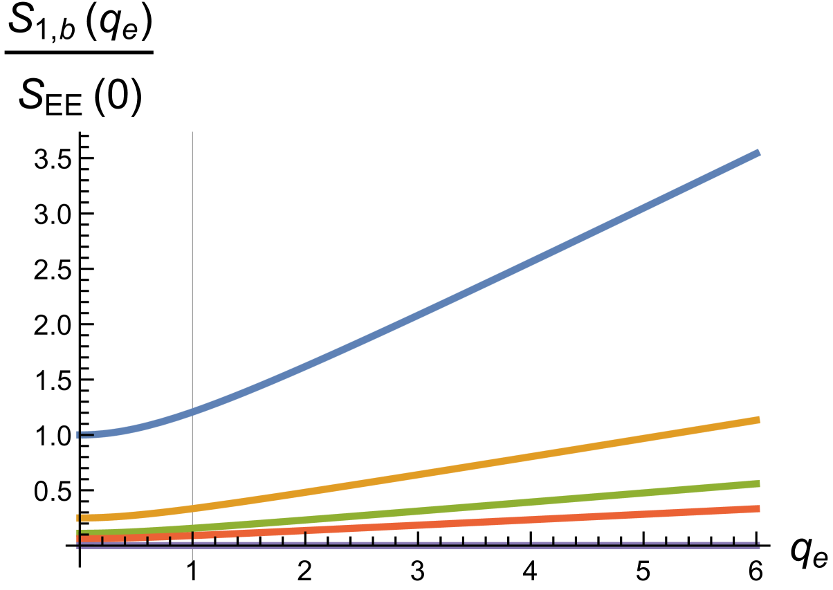
(a)

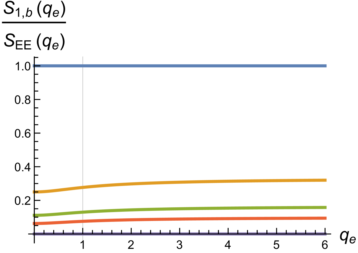
(b)

Figure 11: A plot of $S_{1,b}(q_{e})$ as a function of $q_{e}$ for various fixed values of $b$. (a) Normalized by $S_{1,1}(0)$. (b) $S_{1,1}(q_{e})$. In both plots $b=1$ (blue), $b=2$ (orange), $b=3$ (green), $b=4$ (red), and $b=100$ (purple).

As in $d\geq 3$, there exists a critical value of the Rényi index $q_{c}$ where $S_{q,b}$ diverges. Specifically,

$$q_{c}=\left[1+\frac{x_{11}}{2}(b^{2}-1)\left(1-\frac{q_{e}^{2}}{4x_{11}^{2}}\right)\right]^{-1}\;.$$ (95)

Notice that the sign of $q_{c}$ depends on whether $b<1$ since for any value of $q_{e}\geq 0$, $1-q^{2}_{e}/4x_{11}^{2}>0$. Note, we do not find any change in this behavior as $q_{e}$ exceeds the unitarity bound $q_{e}^{2}>4$.

We have plotted the behavior of $S_{1,b}(q_{e})$ for a range of $q_{e}$ at various fixed values of $b$ in Figure 11. From Figure 11 we observe that, when normalized by $S_{1,1}(0)$, $S_{1,b}(q_{e})$ clearly grows linearly as a function of $q_{e}$, and as $b\to\infty$, $S_{1,b}(q_{e})$ approaches zero. The linear behavior is markedly different from the exponential growth, as seen in Figure 2. A similar observation was made for $S_{q}(q_{e})$ in Belin:2013uta . In Figure 12 we plot the behavior of $S_{1,b}(q_{e})$ as a function of $b$ for fixed values of $q_{e}$, and also $S_{q,2}(q_{e})$. We see $S_{1,b}(q_{e})$ has similar features as its higher dimensional counterparts, while $S_{q,2}(q_{e})$ displays notably different behavior; specifically we see no divergence and an initial logarithmic growth to a finite constant value.

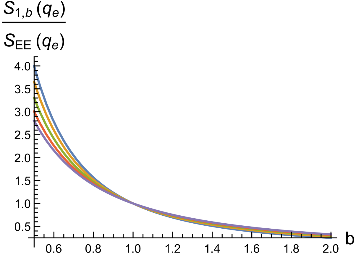
(a)

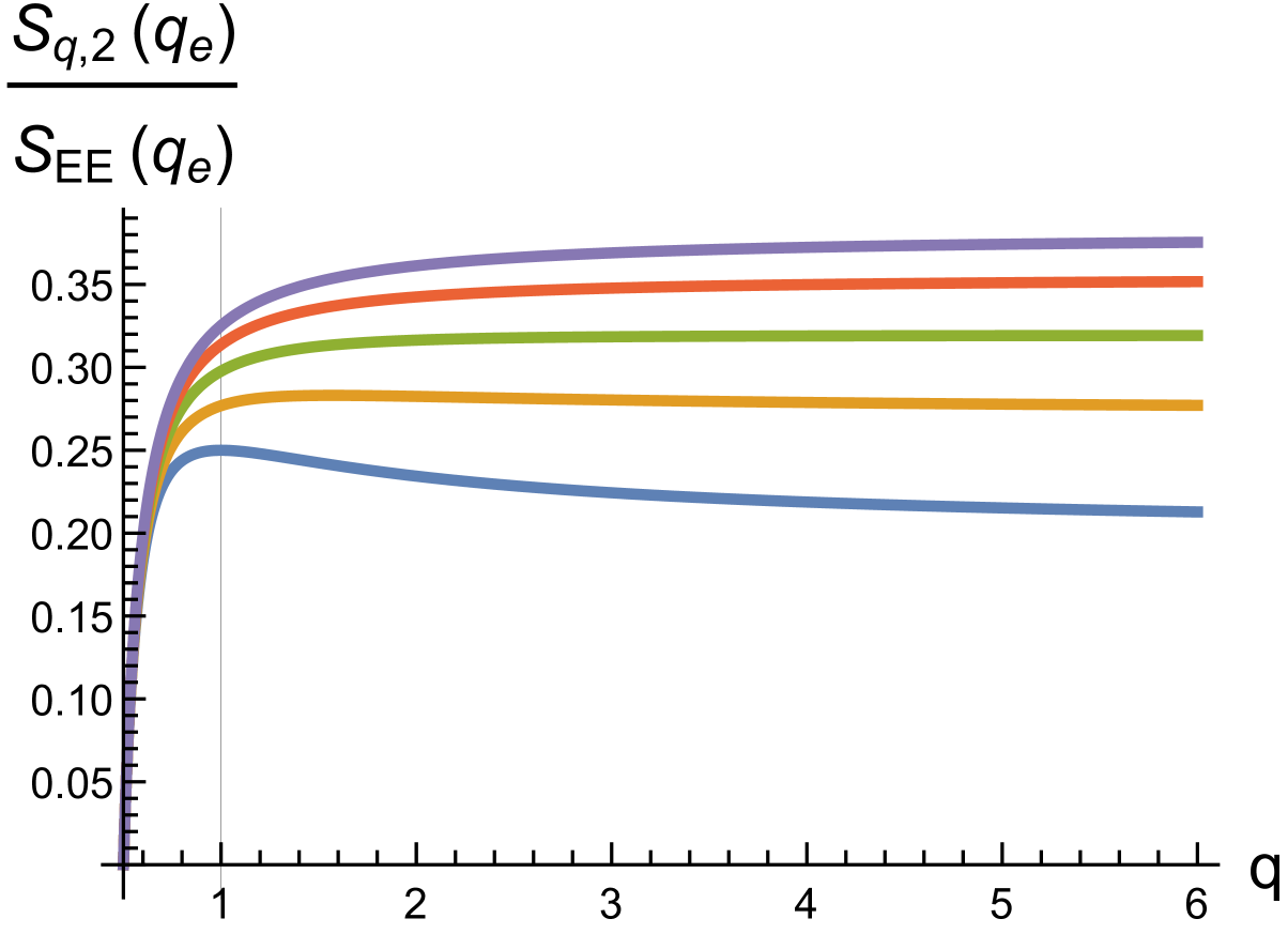
(b)

Figure 12: (a) $S_{1,b}(q_{e})$ as a function of $b$ for various fixed values of $q_{e}$. (b) $S_{q,2}(q_{e})$ as a function of $q$ for various fixed values of $q_{e}$. In both cases $q_{e}=0$ (blue), $q_{e}=1$ (orange), $q_{e}=2$ (green), $q_{e}=4$ (red), and $q_{e}=10$ (purple).

Note we do not see any peculiar behavior for values of $q^{2}_{e}\geq 4$, i.e., beyond the unitarity bound uncovered in Johnson:2019wcq . As we will discuss in more detail later on, this is because we are working with a fixed electrostatic potential.

As in the $d\geq 3$ case, there are potentially special values of $b=b(q)$. Perhaps the most interesting choice of $b$ is $b=q^{-1}$. In this case $x_{qq^{-1}}=x_{11}$, and we find $S_{q,q^{-1}}(q_{e})=0$, agreeing with the uncharged case in $d=2$ Johnson:2018bma . Moreover, it was this particular finding that led to the interpretation of $b$ as a Rényi index, for which $b=q^{-1}$ undoes the $q$-replicas when calculating the Rényi entropy via the replica trick. As we will examine shortly, we will be able to arrive to the same interpretation for the charged system.

Lastly, of interest is when we Wick rotate $q_{e}\to iq^{E}_{e}$. In doing so we have the horizon radius at which $T=T_{0}/q$ and $p=b^{2}p_{0}$,

$$x_{qb}^{E}=\frac{1}{2qb}(1+\sqrt{1-(qbq_{e}^{E})^{2}})\;.$$ (96)

To maintain real solutions, we require $(q_{e}^{E})^{2}<\frac{1}{q^{2}b^{2}}$, telling us that the charge $q_{e}^{E}$ is allowed a finite range of values. Moreover, we may find from $x_{qb}^{E}$ that $(2qbx_{qb}^{E}-1)^{2}+q^{2}b^{2}(q_{e}^{E})^{2}=1$, such that we parameterize the charge $q_{e}^{E}$ via

$$x_{qb}^{E}=\frac{1+\cos\phi}{2qb}\;,\quad q_{e}^{E}=\frac{\sin\phi}{qb}\;.$$ (97)

Thus, similar to the usual charged Rényi entropy $S_{q,1}(q_{e})$ Belin:2013uta , we expect a free field calculation of $S_{q,b}(q_{e})$ will likewise have $q_{e}^{E}$ taking only a finite range of values.

5.3 Field Theory Interpretation

In Section 4 we considered the field theory interpretation of the extended Rényi entropy $S_{q,b}(\mu)$, whereby we made a generalization of the CHM map (52). As in the uncharged case, a direct field theory computation of $S_{q,b}(\mu)$ is difficult and lacking for dimensions $d\geq 3$. However, the calculation for $S_{q}(\mu_{E})$ has been established in $d=2$ for a free massless Dirac fermion $\psi$ on an infinite line reduced to an interval $y\in[u,v]$ Belin:2013uta . Formally this is accomplished by evaluating the partition function for $\psi$ on a $q$-sheeted Riemann surface. The partition function may be expressed in terms of a correlation function of generalized twist operators inserted at the endpoints of the interval $y=[u,v]$. We will only summarize the details of the field theory calculation here, for more a through treatment see Belin:2013uta .

In the uncharged case with $b=1$ the $q$-sheeted Riemann surface is described by the coordinate $w=y+i\tau$, such that the interval $[u,v]$ introduces a branch cut where $\tau$ is the periodic time coordinate with period $\beta=1/T_{0}$. Introducing a complex coordinate $\zeta=(w-u)/(w-v)$, a conformal transformation places the ends of the branch cut at $y=0$ and $y=\infty$, where each time we cross the branch cut we move from one sheet to the next. The fermion field $\tilde{\psi}_{k}$ ($k=1,...,q$) on the $k$th sheet will satisfy a set of boundary conditions coming from a phase shift in $\tilde{\psi}_{k}$ as we move from one sheet to the next, namely,

$$\tilde{\psi}_{m}(e^{2\pi i}(w-u))=e^{2\pi im/q}\tilde{\psi}_{m}(w-u)\;,\quad\tilde{\psi}_{m}(e^{2\pi i}(w-v))=e^{-2\pi im/q}\tilde{\psi}_{m}(w-v)\;,$$ (98)

where $m=\{-(q-1)/2,-(q-1)/2+1...,(q-1)/2\}$. The phase shifts in the fermion fields are generated by the usual twist operators $\sigma_{m/q}$ and $\sigma_{-m/q}$, with conformal weights $h_{q/m}=c(m^{2}/q^{2})$. The twist operator $\sigma_{m/q}$ only acts on each $\tilde{\psi}_{m}$. The partition function $Z_{q}=\text{tr}\rho_{v}^{q}$ is proportional to the correlation function $\langle\sigma_{q}(u)\sigma_{-q}(v)\rangle\sim|(u-v)/\epsilon|^{-(h_{q}+h_{-q})}$, where $\epsilon$ is a UV regulator, and $\sigma_{q}$ is the full twist operator, $\sigma_{q}=\prod_{m}\sigma_{m/q}$. Here $h_{q}=h_{-q}$ is the conformal dimension of twist operator $\sigma_{q}$, given by

$$h_{q}=\sum_{m=-\frac{(q-1)}{2}}^{\frac{(q-1)}{2}}h_{q/m}=\frac{cq}{12}\left(1-\frac{1}{q^{2}}\right)\;.$$ (99)

In this way, the relevant calculation of the uncharged Rényi entropy $S_{q}=\frac{1}{q-1}(q\log Z_{1}-\log Z_{q})$ is reduced to finding the conformal dimension.

The conformal dimension $h_{q}$ (99) can also be found working with a single copy of the complex plane described by coordinate $z$ via the uniformization map of the $q$-sheeted Riemann surface, $z=\zeta^{1/q}$. In this scenario the conformal weight $h_{q}$ arises from the anomaly term – proportional to a Schwarzian derivative – of the stress energy tensor $T(w)$ associated with the CFT on the Riemann surface.

When $b\neq 1$, $S_{q,b}$ is found by computing the partition function $\text{tr}(\rho^{(b)}_{v})$ again using the correlator of twist fields. The details using the uniformization map are largely the same; all that changes is the conformal weight, which corresponds to altering the uniformization map to $z=\zeta^{1/qb}$, leading to $h^{(b)}_{q}=\frac{c}{12}q(1-\frac{1}{q^{2}b^{2}})$ Johnson:2018bma . Importantly, $h^{(b)}_{q}\neq h_{qb}$. In light of (99), interestingly we may reproduce $h^{(b)}_{q}$ simply by

$$h^{(b)}_{q}(q_{e}=0)=\frac{1}{b}h_{qb}\;.$$ (100)

Correspondingly, $h_{qb/m}=c(m^{2}/(qb)^{2})$, with integer $m=[-(qb-1)/2,(qb-1)/2]$, and the boundary conditions for the fermion field $\tilde{\psi}_{m}$ satisfy (98), however, replacing $q\to qb$.

Notice the effect of when $b=q^{-1}$. From the perspective of the uniformization map, $z=\zeta$, and $h^{(q^{-1})}_{q}=0$, such that $S_{q,q^{-1}}(q_{e}=0)=0$ in $d=2$. That is, $b$ ‘undoes’ the $q$-replicas. This can also be seen from the modified boundary conditions for the fermion field (98): as $b$ undoes $q$ there are no phase changes for the fermion, corresponding to $m=0$, and consequently $h_{m/qq^{-1}}=0$. We point out, moreover, when we send $q\to 1$ and keep $b$, then $\tilde{\psi}_{m}$ will undergo phase changes as we move from each $k$th replica sheet, where now $k=1,...,b$.

Let’s now move on and consider charged CFTs. For the fermion system described above, it is natural to introduce a charge associated with global phase rotations of $\psi\to e^{i\theta}\psi$. The charged Rényi entropies are similarly computed as before, however, the introduction of a Wilson loop associated with an imaginary chemical potential $\mu_{E}$ leads to additional phase shift in the boundary conditions for fermion fields on the $m$th sheet $\tilde{\psi}_{m}$,

$$\tilde{\psi}_{m}(e^{2\pi i}(w-u))=e^{2\pi im/q+i\mu_{E}}\tilde{\psi}_{m}(w-u)\;,\quad\tilde{\psi}_{m}(e^{2\pi i}(w-v))=e^{-2\pi im/q-i\mu_{E}}\tilde{\psi}_{m}(w-v)\;.$$ (101)

The phase shifts arise from the introduction of twist operators $\sigma_{m/q,\mu_{E}},\sigma_{-m/q,-\mu_{E}}$ at the endpoints of the branch cut with the same conformal weight

$$h_{q/m}(\mu_{E})=c\left(\frac{m}{q}+\frac{\mu_{E}}{2\pi}\right)^{2}\;.$$ (102)

Since there is an ambiguity in defining the phase shifts (101) modulo $2\pi$, we are free to add an integer $\ell_{m}$ to $h_{q}(\mu_{E})$. For small charge, i.e., small $\mu_{E}$, all $\ell_{m}$ may be set to zero, keeping the range of $m\in[-\frac{q-1}{2},\frac{q-1}{2}]$. Consequently, the expression for $S_{q}(\mu_{E})$ for small $\mu_{E}$ is equal to $S_{q}(\mu_{E}=0)$. As $\mu_{E}$ increases, however, not all $\ell_{m}$ can be set to zero, leading to phase transitions in $S_{q}(\mu_{E})$ occuring whenever $\mu_{E}=\frac{\pi}{q}(2k+1)$ for integer $k$.

Now let’s turn on $b$ for $q_{e}\neq 0$. As in the neutral case, we can write down what $h^{(b)}_{q}(q_{e})$ in terms of $h_{qb/m}(q_{e})$, where now the range of $m$ is modified. Notice when $b=q^{-1}$, $h^{(b)}_{q}(q_{e})\neq 0$ for non-zero charge. In fact, even for small charge $q_{e}$, where we can likewise set the integer $\ell_{m}$ (such that $m\in[-\frac{qb-1}{2},\frac{qb-1}{2}]$), the conformal weight of twist operators $\sigma_{q}^{(b)}$ will be non-zero. Moreover, for larger $q^{E}_{e}$ not all $\ell_{m}$ can be set to zero. This reveals phase transitions in $S_{q,b}(q^{E}_{e})$ whenever $q_{e}^{E}=\frac{\pi}{qb}(2k+1)$ for integer $k$, matching what we found from holographic considerations (97).

While we have not performed an explicit field theory calculation for the conformal weight $h^{(b)}_{q}(q_{e})$, we can compute it holographically. This is accomplished using the difference in enthalpies $M(T_{0},p_{0},q_{e}=0)-M(T_{0}/q,b^{2}p_{0},q_{e})$ (59) using the extended thermodynamics of the charged BTZ black hole (79)

$$h^{(b)}_{q}(q_{e})=\frac{qc}{12}\left[(1-x_{qb}^{2})+\frac{q_{e}^{2}}{2}\log(x_{qb})\right]\;.$$ (103)

When $q_{e}=0$ we recover the uncharged result in $d=2$ Johnson:2018bma . Notice that when $b=q^{-1}$, $h^{(b)}_{q}(q_{e})\neq 0$, unlike the neutral case. Naively we might be alarmed by this since $S_{q,q^{-1}}(q_{e})=0$, however, a non-zero conformal weight when $b=q^{-1}$ is completely compatible with the result $S_{q,q^{-1}}=0$, as we now briefly demonstrate.

From the extended CHM map (52) it is easy to write down $S_{q,b}(q_{e})$ in $d=2$ as

$$S_{q,b}(q_{e})=\left[1+\frac{qx_{11}}{2}\frac{(b^{2}-1)}{q-1}\left(1-\frac{q_{e}^{2}}{4x_{11}^{2}}\right)\right]^{-1}\frac{1}{q-1}(q\log Z_{11}-\log Z_{qb})\;,$$ (104)

with

$$Z_{qb}=\left(\frac{|u-v|}{\epsilon}\right)^{-2h^{(b)}_{q}(q_{e})}\;.$$ (105)

In the neutral case, $b=q^{-1}$ has $\log Z_{11}=0$ since $h^{(q^{-1})}_{q}=0$. For $q_{e}\neq 0$, while $\log Z_{11}\neq 0$, we nonetheless find (104) with the conformal weight (103) reproduces the charged entropy $S_{q,b}(q_{e})$ (88).

It is worth pointing out that for small $q_{e}$

$$h_{q}^{(b)}(q_{e})\approx\frac{c}{12}q\left(1-\frac{1}{q^{2}b^{2}}\right)-\frac{c}{24}q_{e}^{2}q[1+\log(qb)]\;.$$ (106)

Substituting this into (104) we recover, to leading order the neutral limit of $S_{q,b}$

$$S_{q,b}(q_{e})=\frac{1}{[q-1+\frac{q}{2}(b^{2}-1)]}\left[q\left(1-\frac{1}{q^{2}b^{2}}\right)+\frac{qq_{e}^{2}}{2}\log(qb)\right]\frac{c}{6}\log\left(\frac{|u-v|}{\epsilon}\right)\;.$$ (107)

Meanwhile for large $q_{e}$, the conformal weight (103) becomes

$$h_{q}^{(b)}(q_{e})=\frac{cq}{12}\left[\left(1-\frac{q_{e}^{2}}{4}\right)+\frac{q_{e}^{2}}{2}\log\left(\frac{q_{e}}{2}\right)\right]\;.$$ (108)

Intriguingly, when we saturate the unitarity bound (83), where $q_{e}=2$, the conformal weight vanishes. However, as noted above, $\lim_{q_{e}\to\infty}S_{q,b}(q_{e})\to 0$, where we see no interesting behavior for the specific value $q_{e}=2$, even when $q_{e}\gg(qb)$, with $q$ or $b$ smaller than one.

6 Gravity Dual of Extended Rényi Entropy

In the context described here, the holographic dual of the Rényi entropy is the difference in free energies of an appropriate AdS black hole. More generally, for holographic CFTs dual to Einstein gravity in the bulk, a quantity related to the Rényi entropy, which we will call the modified Rényi entropy and denote as $\tilde{S}_{q}$, has been shown to satisfy an area law analogous to the Ryu-Takayanagi proposal Dong:2016fnf

$$\tilde{S}_{q}\equiv q^{2}\partial_{q}\left(\frac{q-1}{q}S_{q}\right)=\frac{\text{Area(Cosmic Brane)}_{q}}{4G_{N}}\;.$$ (109)

The ‘cosmic brane’ is a (bulk) codimension-2 surface homologous to the boundary entangling region, with tension $T_{q}=\frac{q-1}{4qG_{N}}$, and backreacts on the ambient background geometry by generating a conical deficit Fursaev:1995ef . In the limit $q\to 1$, where the tension $T_{q}$ vanishes, $\tilde{S}_{q}$ collapses to the von Neumann entropy, where the cosmic brane settles to the minimal Ryu-Takayanagi surface. Therefore, while in a general setting the Rényi entropy $S_{q}$ may not have a natural bulk interpretation, the modified Rényi entropy $\tilde{S}_{q}$ naturally satisfies an area law.

The modified entropy $\tilde{S}_{q}$ is derived following the method developed by Lewkowycz:2013nqa to derive the Ryu-Takayanagi formula (see Fursaev:2013fta for a related approach). This is accomplished by relating the partition function $Z[M_{q}]$ of the QFT on the branched cover $M_{q}$ formed from $q$-replicas of the $q=1$ boundary spacetime $M_{1}$ to the on-shell Euclidean action $I_{\text{Bulk}}[B_{q}]$ of the dominant bulk solution $B_{q}$ with boundary $M_{q}$ via

$$Z[M_{q}]=e^{-I_{\text{Bulk}}[B_{q}]}\;.$$ (110)

Due to the $\mathbb{Z}_{q}$ replica symmetry, locality of the bulk action leads to $I_{\text{Bulk}}[B_{q}]=qI_{\text{Bulk}}[\hat{B}_{q}]$, where $\hat{B}_{q}$ is the orbifold $\hat{B}_{q}\equiv B_{q}/\mathbb{Z}_{q}$. Consequently, the boundary Rényi entropy is given in terms of the bulk action Lewkowycz:2013nqa

$$S_{q}=\frac{q}{q-1}\left(I_{\text{Bulk}}[\hat{B}_{q}]-I_{\text{Bulk}}[\hat{B}_{1}]\right)\;.$$ (111)

Evaluating $\partial_{q}I_{\text{Bulk}}[\hat{B}_{q}]$ in the polar coordinate system $ds^{2}=dr^{2}+\frac{r^{2}}{q^{2}}d\phi^{2}+g_{ij}dy^{i}dy^{j}$, where $y^{i}$ and $g_{ij}$ are the coordinates and metric on the brane, respectively, and $\phi\in[0,2\pi]$, we arrive at (109) Dong:2016fnf . Recently it was shown the addition of a Nambu-Goto brane action used to account for $\tilde{S}_{q}$ necessarily arises from including a boundary Hayward term in the full bulk gravity action Botta-Cantcheff:2020ywu .

The entropy $\tilde{S}_{q}$ also has a thermodynamic interpretation. Writing the free energy as $F_{q}=-\frac{1}{q}\log\text{tr}\rho^{q}$, with temperature $\tilde{T}=1/q$, we see $\tilde{S}_{q}=-\frac{\partial F_{q}}{\partial\tilde{T}}$. For the case of spherical entangling regions, as explored here, we are really studying the integrated version of (109). Moreover, just as the quench interpretation of $S_{q}$ holds for charged CFTs, the modified entropy $\tilde{S}_{q}$ area relation is robust enough to adequately describe globally charged systems. This can be easily seen from the fact that $S_{q}(\mu)$ satisfies the inequality

$$\tilde{S}_{q}(\mu)\equiv q^{2}\partial_{q}\left(\frac{q-1}{q}S_{q}(\mu)\right)\geq 0\;.$$ (112)

Without going through the details, this is equal to the area of a (charged) cosmic brane.

It is natural to ask whether the extended Rényi entropy $S_{q,b}$ has a similar dual formulation. To study this, let’s first consider when $q=1$, and let $\mu=0$. Then, defining our Gibbs free energy as $G_{1,b}=-\log[\text{tr}\rho_{A}^{(b)}]$ (where the temperature $T=1/q=1$ here), we find it is natural to define the modified entropy $\tilde{S}_{1,b}$ given in terms of a derivative of $G_{1,b}$ with respect to $pV/S=\frac{1}{2}(d-1)b^{2}$:

$$\tilde{S}_{1,b}\equiv-\frac{\partial G_{1,b}}{\partial(pV/S)}=\frac{1}{(d-1)b}\partial_{b}[(b^{2}-1)S_{1,b}]\;.$$ (113)

From the inequalities (46) for $S_{1,b}$ we have $\tilde{S}_{1,b}$ is never negative, similar to $\tilde{S}_{q}$. Also note $\tilde{S}_{1,1}=S_{EE}$.

Analogously, we can define the modified entropy $\tilde{S}_{q,b}$ as

$$\begin{split}\tilde{S}_{q,b}&\equiv\frac{1}{2}\left(q^{2}\partial_{q}+\frac{1}{(d-1)b}\partial_{b}\right)\left[\left(\frac{(q-1)}{q}+\frac{(d-1)x_{11}(b^{2}-1)}{2}\right)S_{q,b}\right]\\ &=-\frac{1}{2}\left(\frac{\partial}{\partial T}+\frac{\partial}{\partial(pV/S)}\right)G_{q,b}\;.\end{split}$$ (114)

It is easy to check that this modified entropy is positive for all $q,b>0$. The overall factor of $1/2$ normalizes $\tilde{S}_{q,b}$ such that $\lim_{q,b\to 1}\tilde{S}_{q,b}\to S_{EE}$. We emphasize, however, the limits $q,b\to 1$ and the $\partial_{q},\partial_{b}$ derivatives do not commute, e.g., taking the limit $b\to 1$ does not lead to $\tilde{S}_{q}$. Thus, $\lim_{b\to 1}\tilde{S}_{q,b}\neq\tilde{S}_{q}$. To include charge, all that is required is we modify $pV/S=(d-1)b^{2}x_{11}/2$.

In light of the above discussion, it is natural to wonder whether the extended modified entropy $\tilde{S}_{q,b}$ has an area-law prescription similar to $\tilde{S}_{q}$ (109). Without a more precise understanding of the field theory interpretation of $S_{q,b}$ it is unclear whether this is the case. We can make some progress, however, when we consider the $d=2$ limit, where the field theory interpretation has been more insightful than in higher dimensions, where we saw that $S_{1,b}$ can be built by evaluating the CFT partition function on a $b$-replica Riemann (boundary) surface. Indeed, this suggested $G_{q,b}\sim\log[\text{tr}(\rho_{w}^{qb})]$, for some density matrix $\rho_{w}$ Johnson:2018bma .

Analogously then, we may formally follow the method used in Lewkowycz:2013nqa ; Dong:2016fnf to try and develop an area law prescription for our modified entropy $\tilde{S}_{q,b}$. For simplicity we consider the neutral limit. Let $M_{q,b}$ be the branched cover formed by $q,b$ replicas of the $q=b=1$ boundary spacetime $M_{1,1}$, and let $Z[M_{q,b}]$ be the partition function of the CFT on this replicated space. We then formally relate the CFT partition function to the on-shell bulk Euclidean action $Z[M_{q,b}]=e^{-I_{\text{Bulk}}[B_{q,b}]}$ where $B_{q,b}$ is the dominant bulk solution with boundary $M_{q,b}$. Our studies from $d=2$ suggest there is a $\mathbb{Z}_{qb}$ symmetry, such that $I_{\text{Bulk}}[B_{q,b}]=qbI_{\text{Bulk}}[\hat{B}_{q,b}]$, with $\hat{B}_{q,b}=B_{q,b}/\mathbb{Z}_{qb}$. Then, from the form of $S_{q,b}$ in (54), where $S_{q,b}\sim q\log Z[M_{1,1}]-\log Z[M_{q,b}]$, we have

$$\left[\frac{(q-1)}{q}+\frac{1}{2}(b^{2}-1)\right]S_{q,b}=\left(bI_{\text{Bulk}}[\hat{B}_{q,b}]-I_{\text{Bulk}}[\hat{B}_{1,1}]\right)\;.$$ (115)

Here we take the bulk action to be the same as given in Dong:2016fnf , $I_{\text{Bulk}}=-\frac{1}{16\pi G_{N}}\int d^{3}X\sqrt{G}R$, $X$, $G_{\mu\nu}$, and $R$ are, respectively, denote the coordinates, metric and Ricci scalar of the bulk geometry. If we leave $b$ fixed, we find the $q$ derivative of this object is proportional to the area of a cosmic brane, up to a factor of $q^{-2}$ (the $b$ index is cancelled), where we have evaluated $\partial_{q}I_{\text{Bulk}}[\hat{B}_{q,b}]$ with the polar coordinate system $ds^{2}=dr^{2}+\frac{r^{2}}{q^{2}b^{2}}d\phi^{2}+g_{yy}(y)dy^{2}$. Explicitly Dong:2016fnf ,

$$\partial_{q}I_{\text{Bulk}}[\hat{B}_{q,b}]=\frac{1}{16\pi G_{N}}\int d^{2}yd\phi\sqrt{\gamma}\hat{n}^{\mu}(\nabla^{\nu}\partial_{q}G_{\mu\nu}-G^{\nu\rho}\nabla_{\mu}\partial_{q}G_{\nu\rho})\;,$$ (116)

where we evaluate the the integral on a thin codimension-1 tube around the cosmic brane, with $\gamma$ being the induced metric on this tube and $\hat{n}^{\mu}=\partial^{\mu}_{r}$ is the outward pointing normal away from the brane. Then, in our polar coordinae system, where $\hat{n}^{\mu}\nabla^{\nu}\partial_{q}G_{\mu\nu}=\frac{2}{qr}$ we find

$$\partial_{q}\left[\frac{(q-1)}{q}+\frac{1}{2}(b^{2}-1)\right]S_{q,b}=b\partial_{q}I_{\text{Bulk}}[\hat{B}_{q,b}]=\frac{1}{q^{2}}\frac{\text{Area(Cosmic Brane)}_{q,b}}{4G_{N}}\;.$$ (117)

Taking the $b\to 1$ limit on the left hand side simply yields $\tilde{S}_{q}$.

Alternatively, note that a $b$-derivative on (115) leads to an additional term

$$\partial_{b}\left(\left[\frac{(q-1)}{q}+\frac{1}{2}(b^{2}-1)\right]S_{q,b}\right)=b(\partial_{b}I_{\text{Bulk}}[\hat{B}_{q,b}])+I_{\text{Bulk}}[\hat{B}_{q,b}]\;.$$ (118)

Since $g_{yy}=g_{yy}(y)$, the $I_{\text{Bulk}}[\hat{B}_{q,b}]$ vanishes on-shell, and we find the remaining term is proportional to the area of the cosmic brane. Specifically,

$$qb\partial_{b}\left(\left[\frac{(q-1)}{q}+\frac{1}{2}(b^{2}-1)\right]S_{q,b}\right)=\frac{\text{Area(Cosmic Brane)}_{q,b}}{4G_{N}}\;.$$ (119)

Taking the $q\to 1$ limit on the left hand side, we recognize this quantity as $\tilde{S}_{1,b}$ (113).

Substituting results (117) and (119) into (114) yields an area-law relation for $\tilde{S}_{q,b}$:

$$\tilde{S}_{q,b}=\frac{1}{2}\left(1+\frac{1}{qb^{2}}\right)\frac{\text{Area(Cosmic Brane)}_{q,b}}{4G_{N}}\;.$$ (120)

As noted before, $\lim_{q\to 1}\tilde{S}_{q,b}\neq\tilde{S}_{1,b}$, however, when $q,b\to 1$ we recover $\tilde{S}_{1,1}=S_{EE}$, with $S_{EE}$ given by the Ryu-Takayanagi formula.

On one hand, the result (120) is not particularly surprising in that our extended Rényi entropy follows from the thermal entropy of a hyperbolically sliced black hole, whose horizon is the minimal Ryu-Takaynagi surface. Alternately, our latter derivation did not make explicit use of the black hole geometry, but instead that of the geometry near the cosmic brane, likewise characterized by a Nambu-Goto action. We should also stress that while our above derivation was a special case, (neutral and $d=2$) we expect that we will find a similar area prescription for $\tilde{S}_{q,b}$ when the dual CFT is charged. Working in higher dimensions may be more difficult, as the additional term $I_{\text{Bulk}}[\hat{B}_{q,b}]$ may lead to a non-trivial modification to the area law contribution to $\tilde{S}_{1,b}$. It would be interesting to persue this further in the future.

7 Summary and Future Work

Here we have extended the charged holographic Rényi entropy $S_{q}(\mu)$ of a globally charged holographic CFT characterized by a chemical potential $\mu$. Our generalization was motivated by the extended black hole thermodynamics of charged AdS black holes with hyperbolically sliced horizons. The resulting quantity $S_{q,b}(\mu)$ can be understood as a single parameter deformation of the usual Rényi entropy $S_{q}(\mu)$, where $b$ corresponds to changes in the pressure of a black hole whose charge and electrostatic potential is proportional to $\mu$. Collectively our work extends both Belin:2013uta and Johnson:2018bma . We exhaustively analyzed the behavior of $S_{q,b}(\mu)$ as a function of each of its parameters, $q,b$, and $\mu$, and found that $S_{q,b}(\mu)$ behaves in many ways like a Rényi entropy. Of particular interest is the $q\to 1$ limit $S_{1,b}$, which we showed acts like the usual Rényi entropy $S_{q}$, satisfying a similar set of inequalities $S_{q}$ is expected to satisfy. Our analysis suggests an apt field theoretic interpretation of $b$ is that of a genuine Rényi index. This conclusion was confirmed by our holographic computations of the conformal weights $h^{(b)}_{q}$ of higher dimensional twist operators, as well as a field theoretic calculation of $h^{(b)}_{q}$ in the $d=2$ case, where the charged AdS black hole geometry is that of a charged BTZ black hole. Ultimately we found that many of the general features of the extended Rényi entropy are present even in the presence of a global charge, a result similar to what was observed in Belin:2013uta . Finally, we introduced a modified entropy $\tilde{S}_{q,b}$ and found an area law prescription in terms of a backreacting cosmic brane when restricted to $d=2$.

Let’s now outline possible avenues for future work.

CFTs Dual to Higher Curvature Theories of Gravity

Here we only considered CFTs that are dual to general relativity. There are, of course, holographic CFTs whose bulk description is given by higher curvature theories of gravity, e.g., Gauss-Bonnet or quasi-topological gravity. In fact, the neutral holographic Rényi entropy $S_{q}$ has already been studied in the context of such bulk theories Hung:2011nu , where the Rényi entropy is a complicated non-linear function of the generalized central charge $a_{d}^{\ast}$ Myers:2010tj , computed using the Wald entropy of the black hole. It would be interesting to see what effects a global charge would introduce, both for $S_{q}$ and its extension $S_{q,b}$, for example, how the conformal weights of the generalized twist operators behave.

As with the bulk theory we considered here, special attention would need to be given to theories in $d=2$ dimensions. This is because determining the generalized central charge $a_{d}^{\ast}$ requires the solution of the bulk theory to be locally AdS, for which the charged BTZ black hole is not. It turns out when the bulk theory is Einstein-Maxwell the expression for $a_{d}^{\ast}$ does not change for the charged BTZ black hole because the form of the Wald entropy functional satisfies in effect the locally AdS symmetry condition. For higher curvature theories of gravity in $d=2$, such as new massive gravity and its generalizations Bergshoeff:2009hq ; Bergshoeff:2009aq ; Sinha:2010ai , we expect understanding how the Rényi entropy depends on the $a_{d}^{\ast}$ will be more elusive.

For the case of $d=2$ it might also be interesting to consider how the extended Rényi entropy $S_{q,b}(q_{e})$ changes when the bulk theory in question is Chern-Simons gravity. It is plausible that $S_{q,b}$ will be independent of the charge $q_{e}$, similar to $S_{q}$ Belin:2013uta , as the gauge potential $A$ does not couple to the metric such that $A$ is constant in the bulk, and without a bulk source this constant is zero. Since $S_{q,b}$, however, depends on both the entropy and the thermodynamic volume $V$, it is conceivable the inclusion of $V$ will lead to a $S_{q,b}$ which still depends on $q_{e}$. It would be interesting to study this scenario as it may provide an example in which the behaviors of $S_{q}$ and $S_{q,b}$ differ dramatically.

Varying Potential, Virasoro Symmetry and Super-entropicity

We considered holographic CFTs with a conserved global charge, described in the grand canonical ensemble with chemical potential $\mu$. For any dimension $d$, this condition translated to working with a charged black hole in the grand canonical ensemble at fixed electrostatic potential $\Phi_{e}$. On the gravity side, it is quite natural to study systems for which the potenial $\Phi_{e}$ or charge $q$ are left unfixed; in fact, the extended thermodynamics of charged AdS black holes is by now well-known to be rich and complex, behaving as a van der Waals fluid Dolan:2011xt ; Kubiznak:2012wp . Allowing the potential $\Phi_{e}$ to vary would immediately change the quench expression for the difference in Gibbs free energies, in which the denominator includes a term $-Q\Delta\Phi_{e}$. However, since $\Phi_{e}\propto\mu$, it is unclear what the field theoretic meaning of this difference in Gibbs free energies corresponds to, as this would imply the global charge of the CFT is not conserved.

Studying the set-up for varying potential $\Phi_{e}$ would be particularly interesting in the $d=2$ case. In fact, note we did not see any peculiar behavior for values of $q^{2}_{e}\geq 4$, i.e., beyond the unitarity bound uncovered in Johnson:2019wcq . Naively we might expect to see a transition in behavior for $q^{2}_{e}$ above and below the unitarity bound considering this is when the BTZ black hole has a thermodynamic instability, and is correspondingly super-entropic. Since we held $\Phi_{e}$ fixed, this corresponds to subtly using the renormalization scheme Cadoni:2007ck . Consequently, the charged BTZ black hole is notably not super-entropic, thermodynamically stable, and, correspondingly, $q^{2}_{e}$ does not affect the unitarity bound of the dual $\text{CFT}_{2}$. Moreover, employing this renormalization scheme has the charged BTZ black hole exhibiting explicit Virasoro symmetry in its asymptotic structure. Effectively, then, allowing $\Phi_{e}$ to vary means we ignore the renormalization scheme, whereby the Virasoro symmetry of the underlying CFT becomes hidden and the black hole becomes super-entropic and thermodynamically unstable. Provided there exists a suitable interpretation of $S_{q}(\mu)$ for varying $\mu$, it would be interesting to see whether the thermodynamic instability affects the Rényi entropy, perhaps leading to new phase transitions in $S_{q}$ in $d=2$. Moreover, we may gain further insight into the microscopic understanding of black hole super-entropicity, building off of the recent work Johnson:2019wcq .

Holographic Phase Transitions

It is well known that charged hyperbolic AdS black holes do not exhibit a Hawking-Page phase transition Cai:2004pz . This can be observed from the Gibbs free energy, which is everywhere negative except in the extremal limit when it becomes zero. Moreover, the specific heat at fixed $\mu$ is always positive. Therefore, the charged topological AdS black hole does not exhibit any phase transitions. As such, the charged Rényi entropy $S_{q}(\mu)$ and its extension $S_{q,b}(\mu)$ do not exhibit any phase transitions induced by the bulk geometry.

In spite of this, when a (charged) light scalar field is present in the bulk, (charged) black holes become unstable in the near extremal limit when the mass of the scalar field is below the BF bound of the $AdS_{2}$ sector of the near horizon geometry. Consequently, the scalar field condenses leading to a hairy black hole, signalling a dual phase transition in the (charged) Rényi entropy Belin:2013dva ; Belin:2014mva . It would be interesting to similarly study the phase transitions of $S_{q,b}$ – both the neutral and charged cases – that arise from the same scalar field condensation, as it may expand our understanding of holographic superconductors. An analytic study of such holographic phase transitions is currently underway.

Information Theoretic Meaning of $S_{q,b}$

Perhaps the most worthwhile future research avenue is to develop a concrete information theoretic interpretation of $S_{q,b}$. Here we exploited the quench definition of the Rényi entropy, and naturally generalized it by replacing the difference in Helmholtz free energies with a difference in Gibbs free energies. As noted in baez:2011 , written as a quench, it is evident $S_{q}$ is proportional to the ‘$q$-derivative’ of the free energy $F(T)$, $S_{q}=-\left(\frac{\partial F}{\partial T_{0}}\right)_{q^{-1}}$, where the $q$-derivative of a function $f$ is defined as

$$\left(\frac{\partial f}{\partial x}\right)_{q}=\frac{f(qx)-f(x)}{(q-1)x}\;.$$ (121)

The $q$-derivative appears often in mathematics literature whenever one ‘$q$-deforms’ some ordinary structure, e.g., $q$-deformed Lie groups produce quantum groups, and is prevalent in the theory of quantum calculus cheung2002 . The $q$-derivative interpretation of information and statistical entropies has been known for some time Abe1997 and continues to be of interest Marinho:2020sbc .

Similarly, we can interpret $S_{1,b}$ as a $q$-derivative of the Gibbs free energy, specifically, $S_{1,b}=-(1/V_{0}/S_{0})\left(\frac{\partial G(T_{0},p_{0})}{\partial p_{0}}\right)_{b^{2}}$. We point out, however, that $S_{q,b}$ is not quite a $b$-deformation of $S_{q}$ in the mathematical sense cheung2002 ; rather $S_{q,b}$ is akin to a simultaneous $q$-derivative of $G(T_{0},p_{0})$ in both of its arguments. It would be interesting to see whether $S_{q,b}$ can be precisely formulated with $q$-calculus, as it applies to more generic thermodynamic systems, and may lead to a new kind of information entropy, whose holographic dual would have an immediate interpretation.

References

- (1) C. V. Johnson, Physical Generalizations of the Rényi Entropy, Int. J. Mod. Phys. D28 (2019) 1950091, [1807.09215].
- (2) S. Ryu and T. Takayanagi, Holographic derivation of entanglement entropy from AdS/CFT, Phys. Rev. Lett. 96 (2006) 181602, [hep-th/0603001].
- (3) V. E. Hubeny, M. Rangamani and T. Takayanagi, A Covariant holographic entanglement entropy proposal, JHEP 07 (2007) 062, [0705.0016].
- (4) J. Bekenstein, Black holes and the second law, Lett. Nuovo Cim. 4 (1972) 737–740.
- (5) S. Hawking, Black hole explosions, Nature 248 (1974) 30–31.
- (6) S. Hawking, Particle Creation by Black Holes, Commun. Math. Phys. 43 (1975) 199–220.
- (7) H. Casini, M. Huerta and R. C. Myers, Towards a derivation of holographic entanglement entropy, JHEP 05 (2011) 036, [1102.0440].
- (8) M. Headrick, Entanglement Renyi entropies in holographic theories, Phys. Rev. D 82 (2010) 126010, [1006.0047].
- (9) J. C. Baez, Renyi Entropy and Free Energy, 1102.2098.
- (10) L.-Y. Hung, R. C. Myers, M. Smolkin and A. Yale, Holographic Calculations of Renyi Entropy, JHEP 12 (2011) 047, [1110.1084].
- (11) A. Belin, L.-Y. Hung, A. Maloney, S. Matsuura, R. C. Myers and T. Sierens, Holographic Charged Renyi Entropies, JHEP 12 (2013) 059, [1310.4180].
- (12) D. Kastor, S. Ray and J. Traschen, Enthalpy and the Mechanics of AdS Black Holes, Class. Quant. Grav. 26 (2009) 195011, [0904.2765].
- (13) D. Kastor, S. Ray and J. Traschen, Smarr Formula and an Extended First Law for Lovelock Gravity, Class. Quant. Grav. 27 (2010) 235014, [1005.5053].
- (14) B. P. Dolan, The cosmological constant and the black hole equation of state, Class. Quant. Grav. 28 (2011) 125020, [1008.5023].
- (15) B. P. Dolan, Where Is the PdV in the First Law of Black Hole Thermodynamics?, pp. 291–316. INTECH, 2012. 1209.1272. 10.5772/52455.
- (16) D. Kubiznak, R. B. Mann and M. Teo, Black hole chemistry: thermodynamics with Lambda, Class. Quant. Grav. 34 (2017) 063001, [1608.06147].
- (17) C. V. Johnson, V. L. Martin and A. Svesko, Microscopic description of thermodynamic volume in extended black hole thermodynamics, Phys. Rev. D 101 (2020) 086006, [1911.05286].
- (18) A. A. Balushi, R. A. Hennigar, H. K. Kunduri and R. B. Mann, Holographic Complexity and Thermodynamic Volume, 2008.09138.
- (19) A. A. Balushi, R. A. Hennigar, H. K. Kunduri and R. B. Mann, Holographic complexity of rotating black holes, 2010.11203.
- (20) A. Belin, L.-Y. Hung, A. Maloney and S. Matsuura, Charged Renyi entropies and holographic superconductors, JHEP 01 (2015) 059, [1407.5630].
- (21) C. Martinez, C. Teitelboim and J. Zanelli, Charged rotating black hole in three space-time dimensions, Phys. Rev. D 61 (2000) 104013, [hep-th/9912259].
- (22) X. Dong, The Gravity Dual of Renyi Entropy, Nature Commun. 7 (2016) 12472, [1601.06788].
- (23) R. C. Myers and A. Sinha, Holographic c-theorems in arbitrary dimensions, JHEP 01 (2011) 125, [1011.5819].
- (24) J. D. Brown and J. W. York, Jr., Quasilocal energy and conserved charges derived from the gravitational action, Phys. Rev. D47 (1993) 1407–1419, [gr-qc/9209012].
- (25) V. Balasubramanian and P. Kraus, A Stress tensor for Anti-de Sitter gravity, Commun. Math. Phys. 208 (1999) 413–428, [hep-th/9902121].
- (26) R. Emparan, C. V. Johnson and R. C. Myers, Surface terms as counterterms in the AdS / CFT correspondence, Phys. Rev. D60 (1999) 104001, [hep-th/9903238].
- (27) C. V. Johnson and F. Rosso, Holographic Heat Engines, Entanglement Entropy, and Renormalization Group Flow, Class. Quant. Grav. 36 (2019) 015019, [1806.05170].
- (28) C. V. Johnson, Holographic Heat Engines, Class. Quant. Grav. 31 (2014) 205002, [1404.5982].
- (29) D. D. Blanco, H. Casini, L.-Y. Hung and R. C. Myers, Relative Entropy and Holography, JHEP 08 (2013) 060, [1305.3182].
- (30) G. Wong, I. Klich, L. A. Pando Zayas and D. Vaman, Entanglement Temperature and Entanglement Entropy of Excited States, JHEP 12 (2013) 020, [1305.3291].
- (31) D. D. Blanco and H. Casini, Localization of Negative Energy and the Bekenstein Bound, Phys. Rev. Lett. 111 (2013) 221601, [1309.1121].
- (32) E. Bianchi and M. Smerlak, Entanglement entropy and negative energy in two dimensions, Phys. Rev. D 90 (2014) 041904, [1404.0602].
- (33) F. Rosso, Holography of negative energy states, Phys. Rev. D 99 (2019) 026002, [1809.04793].
- (34) F. Rosso, Localized thermal states and negative energy, JHEP 10 (2019) 246, [1907.07699].
- (35) L.-Y. Hung, R. C. Myers and M. Smolkin, Twist operators in higher dimensions, JHEP 10 (2014) 178, [1407.6429].
- (36) A. M. Frassino, R. B. Mann and J. R. Mureika, Lower-Dimensional Black Hole Chemistry, Phys. Rev. D 92 (2015) 124069, [1509.05481].
- (37) J. D. Brown and M. Henneaux, Central Charges in the Canonical Realization of Asymptotic Symmetries: An Example from Three-Dimensional Gravity, Commun. Math. Phys. 104 (1986) 207–226.
- (38) J. L. Cardy, Operator Content of Two-Dimensional Conformally Invariant Theories, Nucl. Phys. B270 (1986) 186–204.
- (39) H. W. J. Bloete, J. L. Cardy and M. P. Nightingale, Conformal Invariance, the Central Charge, and Universal Finite Size Amplitudes at Criticality, Phys. Rev. Lett. 56 (1986) 742–745.
- (40) A. Strominger and C. Vafa, Microscopic origin of the Bekenstein-Hawking entropy, Phys. Lett. B379 (1996) 99–104, [hep-th/9601029].
- (41) A. Strominger, Black hole entropy from near horizon microstates, JHEP 02 (1998) 009, [hep-th/9712251].
- (42) S. Carlip, What we don’t know about BTZ black hole entropy, Class. Quant. Grav. 15 (1998) 3609–3625, [hep-th/9806026].
- (43) S. Carlip, Conformal field theory, (2+1)-dimensional gravity, and the BTZ black hole, Class. Quant. Grav. 22 (2005) R85–R124, [gr-qc/0503022].
- (44) M. Cadoni, M. Melis and M. R. Setare, Microscopic entropy of the charged BTZ black hole, Class. Quant. Grav. 25 (2008) 195022, [0710.3009].
- (45) C. V. Johnson, Instability of super-entropic black holes in extended thermodynamics, Mod. Phys. Lett. A 35 (2020) 2050098, [1906.00993].
- (46) M. Cvetic, G. Gibbons, D. Kubiznak and C. Pope, Black Hole Enthalpy and an Entropy Inequality for the Thermodynamic Volume, Phys. Rev. D 84 (2011) 024037, [1012.2888].
- (47) R. A. Hennigar, D. Kubizˇnák and R. B. Mann, Entropy Inequality Violations from Ultraspinning Black Holes, Phys. Rev. Lett. 115 (2015) 031101, [1411.4309].
- (48) R. A. Hennigar, D. Kubizˇnák, R. B. Mann and N. Musoke, Ultraspinning limits and super-entropic black holes, JHEP 06 (2015) 096, [1504.07529].
- (49) D. V. Fursaev and S. N. Solodukhin, On the description of the Riemannian geometry in the presence of conical defects, Phys. Rev. D 52 (1995) 2133–2143, [hep-th/9501127].
- (50) A. Lewkowycz and J. Maldacena, Generalized gravitational entropy, JHEP 08 (2013) 090, [1304.4926].
- (51) D. V. Fursaev, A. Patrushev and S. N. Solodukhin, Distributional Geometry of Squashed Cones, Phys. Rev. D 88 (2013) 044054, [1306.4000].
- (52) M. Botta-Cantcheff, P. J. Martinez and J. F. Zarate, Rényi entropies and area operator from gravity with Hayward term, JHEP 07 (2020) 227, [2005.11338].
- (53) F. Rosso and A. Svesko, Novel Aspects of the Extended First Law of Entanglement, JHEP 08 (2020) 008, [2003.10462].
- (54) E. A. Bergshoeff, O. Hohm and P. K. Townsend, Massive Gravity in Three Dimensions, Phys. Rev. Lett. 102 (2009) 201301, [0901.1766].
- (55) E. A. Bergshoeff, O. Hohm and P. K. Townsend, More on Massive 3D Gravity, Phys. Rev. D 79 (2009) 124042, [0905.1259].
- (56) A. Sinha, On the new massive gravity and AdS/CFT, JHEP 06 (2010) 061, [1003.0683].
- (57) B. P. Dolan, Pressure and volume in the first law of black hole thermodynamics, Class. Quant. Grav. 28 (2011) 235017, [1106.6260].
- (58) D. Kubiznak and R. B. Mann, P-V criticality of charged AdS black holes, JHEP 07 (2012) 033, [1205.0559].
- (59) R.-G. Cai and A. Wang, Thermodynamics and stability of hyperbolic charged black holes, Phys. Rev. D70 (2004) 064013, [hep-th/0406057].
- (60) A. Belin, A. Maloney and S. Matsuura, Holographic Phases of Renyi Entropies, JHEP 12 (2013) 050, [1306.2640].
- (61) P. Cheung and V. Kac, Quantum Calculus, Springer (2002) .
- (62) S. Abe, A note on the q-information theoretic aspect of the generalized entropies in nonextensive physics, Phys. Lett. A 224 (1997) 326.
- (63) A. A. Marinho, G. Viswanathan, F. A. Brito and C. Bezerra, The connection between Jackson and Hausdorff derivatives in the context of generalized statistical mechanics, 2006.00378.