Oort cloud Ecology II: Extra-solar Oort clouds and the origin of asteroidal interlopers

We simulate the formation and evolution of Oort clouds around the 200 nearest stars (within $\sim 16$ pc according to the Gaia DR2) database. This study is performed by numerically integrating the planets and minor bodies in orbit around the parent star and in the Galactic potential. The calculations start 1 Gyr ago and continue for 100 Myr into the future. In this time frame, we simulate how asteroids (and planets) are ejected from the star’s vicinity and settle in an Oort cloud and how they escape the local stellar gravity to form tidal steams. A fraction of $0.0098$ to $0.026$ of the asteroids remain bound to their parent star. The orbits of these asteroids isotropizes and circularizes due to the influence of the Galactic tidal field to eventually form an Oort cloud between $\sim 10^{4}$ and $\sim 2\cdot 10^{5}$ au. We estimate that $\ {\raise-2.15277pt\hbox{$\buildrel<\over{\sim}$}}\ 6$% of the nearby stars may have a planet in its Oort cloud. The majority of asteroids (and some of the planets) become unbound from the parent star to become free floating in the Galactic potential. These sōlī lapidēs  remain in a similar orbit around the Galactic center as their host star, forming dense streams of rogue interstellar asteroids and planets.

The Solar system occasionally passes through such tidal streams, potentially giving rise to occasional close encounters with object in this stream. The two recently discovered objects, 1I/(2017 Q3) ’Oumuamua and 2I/(2019 Q4) Borisov, may be such objects. Although the direction from which an individual sōlus lapis  originated cannot easily be traced back to the original host, multiple such objects coming from the same source might help to identify their origin. At the moment the Solar system is in the bow or wake of the tidal stream of $\sim 10$ of the nearby stars which might contribute considerably to the interaction rate. Overall, we estimate that the local density of such left overs from the planet-formation process contribute to a local density of $1.2\times 10^{14}$ per pc^-3, or $\ {\raise-2.15277pt\hbox{$\buildrel>\over{\sim}$}}\ 0.1$ of the interstellar visitors originate from the obliterated debris disk of such nearby stars.

1 Introduction

The Sun is orbited by a cloud of minor bodies in a spherical distribution between $\sim 10^{4}$ au, and the Hill radius of the Solar system in the Galactic potential. This cloud of objects, generally referred to as the Oort (1950) cloud, may not be unique to the Solar system: other stars may also have their own ’Oort’ clouds (Stern, 1989). The circumstances that lead to the Sun’ Oort cloud could equally well work for many nearby stars, in which case, Oort clouds should be rather common.

Crucial to forming an Oort-like cloud is the presence of a debris disk with relatively massive objects (which we call planets) (Brasser & Morbidelli, 2013). These planets perturb the low-mass minor bodies (which we call asteroids) and drive their eccentricities to high values ($\gg 0.9$) while preserving the closest approach distance to the parent star. Upon each orbit, the asteroid is kicked into a wider and more eccentric orbit while preserving pericenter distance. Eventually, the Galaxy’s tidal field, in which the planetary system orbits, starts to circularize the orbit of the minor body (Duncan et al., 1987). If the tidal field effectively reduces the minor body’s orbital eccentricity, it can remain bound to the parent star and become a member of the local Oort cloud. If the body becomes unbound, it continues as a free-floating asteroid, or sōlus lapis, in the Galactic potential (see Torres et al., 2019a).

The recent arrival of two such sōlī lapidēs, 1I/(2017 Q3) ’Oumuamua (Bacci et al., 2017; Meech et al., 2017a, b) and 2I/(2019 Q4) Borisov (2019) (and maybe even several others Froncisz et al., 2020) in the Solar system makes it worth to study the extent to which an evaporating Oort cloud or circumstellar debris disk of nearby stars contribute to the frequency and characteristics of such objects.

The two observed sōlī lapidēs  were suggested to originate from the Oort clouds of other stars (Portegies Zwart et al., 2018; Raymond et al., 2018; Moro-Martín, 2019), or ejected from a proto-planetary disk (Moro-Martín, 2018), from a binary system Jackson et al. (2018), from a stellar association (Feng & Jones, 2018), or launched by as a tidal fragment (Zhang & Lin, 2020). At least ’Oumuamua and Borisov do not seems to originate from the Sun’s Oort cloud (Meech et al., 2018; Higuchi & Kokubo, 2020).

Several studies have tried to identify the host (Zhang, 2018; Bailer-Jones et al., 2020), but despite the precision of the Gaia-DR2 astrometry (Gaia Collaboration et al., 2018) and the accurate ephemera for the two sōlī lapidēs, this remains uneventful. Another complication in tracing back the interloper to its host star is our lack of knowing the age of the object. Stars as well as sōlī lapidēs  move around in the Galaxy and tracing back one to another can be arduous; much in the same way as it might be hard to identify a dog owner in a dog-walking area.

Nevertheless, there is hope in identifying the sōlus lapis’ host when ejected asteroids linger around the source along it’s Galactic orbit. On the other hand, if sōlī lapidēs  hang around the host star’s orbit, they may not appear at all to be launched from the star itself, but from some distance away. The asteroid may then appear to have come from a somewhat different direction and with a different velocity than the host star, making it hard to connect the two. The orbital velocity of an asteroid in orbit around the parent star at the Hill radius ($dv/v\equiv\delta v\ {\raise-2.15277pt\hbox{$\buildrel<\over{\sim}$}}\ 0.1$ km/s) is considerably smaller than the orbit of the star around the Galactic center ($\sim 240$ km/s). While the host star orbits in the Galactic potential, the low-velocity ejected asteroids will form extended leading and trailing arms along the hosts’ orbit. We call this the proximity argument.

Rather than trying to identify the sōlus lapis’ host star, we use the proximity argument to determine the probable association between the host star and its sōlī lapidēs. We do this by simulating the distribution of asteroids that have become unbound from their parent star. Although these asteroidal tails may be quite extended (several kpc), we limit ourselves to the 200 stars nearest to the Sun (within about 16 pc). We will assume that these stars had a disk of planets and debris sometime in the past. In the simulations, Oort clouds form through planets that eject asteroids. Most of these become unbound and will orbit the Galaxy. We subsequently study the galactic distribution of these ejected asteroids and investigate the probability of them interacting closely with the Solar system.

We study the phase-space distribution of minor bodies from the moment they enter the conveyor belt and are kicked out of the local host-star’s vicinity while sojourning the Milky way Galaxy. Our calculations start by integrating the 200 nearby stars backward in time in the Galactic potential for 1 Gyr. Once calculated backward, they are provided with a planetary system and a population of minor bodies as test particles in a disk. Each star with planets and minor bodies is subsequently integrated forwards in time in the Galactic potential until the current epoch, where they are observed today, near the Sun. We call this the yo-yo scheme. During this orbital calculation we simulate the dynamical evolution of the planets and minor bodies. By that time, each star’s Oort cloud has fully developed, and the majority of minor bodies (and some of the planets) are ejected on Galactic orbits. In this paper, we focus on the distribution of these sōlī lapidēs  in the vicinity of the Sun. For safety, we continue the integration for another 100 Myr after the present time, in case the closest approach with the Sun happens to be in the near future.

2 Methods, initial conditions, and glossary

This numerical study focuses on a hypothetical population of interstellar asteroids that were liberated from their parent stars. After liberation, they float freely in the Galactic potential. Some of these sōlī lapidēs  are welcomed as immigrants in the Solar system or pass through the Oort cloud, but the majority will just hover around orbiting the Galactic center without ever interacting with the Solar system. The calculations depend on several assumptions, and these are reflected, in part, by the initial conditions chosen for this study. We realize that the reader may not be satisfied with some of the choices made, and for this purpose, all the run-scripts, the data, and picture-generating scripts to reproduce this work are available through figshare (Portegies Zwart, 2020a) and github. The source code for the AMUSE framework is available at https://github.com/amusecode/amuse (see Portegies Zwart et al., 2018).

2.1 Glossary of terms

The adopted terminology in this paper may be confusing at times. Therefore a short glossary of terms used is presented.

• Asteroid: low-mass object (compared to the planets) in a bound orbit around a star.

• Conveyor belt: Area in orbital parameter space (in particular semi-major axis and eccentricity) where an asteroid crosses the orbit of one or more of the major planets. These repeated perturbations induce small impulsive velocity-kicks causing the orbits to drift to higher eccentricity and larger semi-major axis while preserving pericenter distance (sometimes called eccentricity pumping). The conveyor belt is indicated in figure 1 as the area between the two black curves.

• Frozen zone: The area in parameter space (semi-major axis and eccentricity) where the orbits of asteroids are insignificantly perturbed by massive bodies (planets or stars) from shorter orbits, or stellar fly-by’s.

• Hill radius: We define the Hill radius as the distance to the star for which the gravitational force is dominated by the star. The Hill distance depends on the stellar mass and its orbit around the Galactic center. The Hill radius depends on direction, which results in an ellipsoid around the star. The force excerted by the star on objects within this volume exceeds the force from the rest of the Galaxy. The Roche radius (Kopal, 1959, p.136) is defined as the radius of a sphere with the same volume as the Hill ellipsoid.

  In figure 1 the Hill radius is presented as the solid red curve, here at roughly $2\cdot 10^{5}$ au. In our calculations, the Hill ellipsoid only considered in post processing the data. During the calculations weather or not an asteroid (or planet) is bound to a star is calculated by integrating the equatios of motion of the star, planets, and asteroids in the potential of the Galaxy. In figure 2 we present the (post-processing) Hill radius for all stars in our simulation to illustrate its variation over time.

• Kuiper cliff: The rather sudden drop in the density of asteroids at the far side of the Edgewordt-Kuiper belt (Edgeworth, 1943; Kuiper, 1951).

• Oort cloud: The Oort cloud is reserved for bound objects but for which a 1 M_⊙  body passing on a hyperbolic orbit at the Hill radius distance induces a relative velocity-perturbation of $\delta v=10^{-5}$. Here we define the relative velocity perturbation $\delta v\equiv|v_{\odot}-v_{\rm Gal}|/v_{\odot}$ as the change in velocity of an object at apocenter in its orbit around a star due to the presence galactic tidal field (see Portegies Zwart & Jilkova, 2015). The inner edge of the Oort cloud is presented in figure 1 by the right-most cyan curve.

• Parking zone: The region between the Kuiper cliff and the Oort cloud. The parking zone in the Solar system is rather empty.

• Rogue planet: Planet that is unbound from any star. Note that strictly speaking, the term free-floating is misleading because they are still bound to the Galaxy.

• Sōlus lapis  (plural: sōlī lapidēs): Asteroid or comet that is not bound to any star but floating freely in the Galaxy. Asteroids to the far side of the Hill radius are generally not bound to the parent star, but have become a member of the Galaxy.

2.2 The simulation environment

The calculations in this study are performed using the Astrophysics Multipurpose Software Environment (Portegies Zwart & McMillan, 2018). AMUSE is a modular language-independent framework for homogeneously interconnecting a wide variety of astrophysical simulation codes. It is built on public community codes that solves gravitational dynamics, hydrodynamics, stellar evolution, and radiative transport. The underlying codes are written in high-performance compiled languages that do not require recompilation when combined with Python scripts. The framework adopts Noah’s Arc philosophy, in which there are at least two codes that solve for the same physics (Portegies Zwart et al., 2009).

Most calculations are carried out using a combination of symplectic direct N-body, test-particle integration, and the tidal field of the Galaxy. For the former two, we use Huayno, which adopts a recursive Hamiltonian-splitting strategy (much like bridge, see Fujii et al., 2007) to generate a symplectic integrator that conserves momentum to machine precision (Pelupessy et al., 2012). For the asteroids, we employed the hold drift-kick-drift scheme in the integrator with a time-step parameter of 0.02 (this results in an integration time-step of about 10-days). We use the GPU enabled version, which employs the Kirin GPU library (Portegies Zwart et al., 2007; Belleman et al., 2014). The direct N-body code and the Galactic potential are coupled using the hierarchical non-intrusive code-coupling strategy discussed in Portegies Zwart et al. (2020) with an interaction time-step of 100 yr.

We ignore stellar mass loss in this study. The most massive star in our sample is 1.23 M_⊙  (HD 346704), which will not leave the main-sequence within $\sim 5.9$ Gyr (for Solar metallicity). This is considerably longer than the time frame over which this study is conducted.

2.3 Reconstructing the debris distribution near the Sun

2.3.1 The yo-yo approach

This study strives to achieve a representative distribution of interstellar asteroids in the Solar system’s vicinity. The yo-yo scheme is carried out in two steps: In the first step (yo), we integrate the known nearby stars backward through time in a representative Galactic potential. In the second step (yo), we integrate these same stars from their back-calculated location in the Galaxy forwards in time to the current epoch. In the second step, each star will have a disk of planets and asteroids which are also integrated in the Galactic potential.

In the next sections, we discuss the following steps in the yo-yo procedure.

• Select the 200 nearby stars used in this study (see Sect. 2.3.2).

• Calculate their Galactic location 1 Gyr ago (see Sect. 2.3.3).

• Supply each star with planets and asteroids (see Sect. 2.3.4).

• Calculate star, planets, and asteroids forwards in time for 1.1 Gyr in the Galactic potential (see Sect. 2.3.5).

2.3.2 Selecting the 200 nearest stars

We start by selecting the 200 stars currently nearest to the Sun. The proper motions, radial velocities, positions, and masses of these stars are taken from the catalog of Torres et al. (2019a, b). The proper motion, distance, and position on the sky in this catalog are taken directly from Gaia DR2 (Gaia Collaboration et al., 2018; Andrae et al., 2018). The radial velocities are derived by cross-matching Gaia DR2 with RAVE-DR5 (Kunder et al., 2017), GALAH DR2 (Buder et al., 2018), LAMOST DR3 (Zhao et al., 2012), APOGEE DR14 (Abolfathi et al., 2018), and XHIP (Anderson & Francis, 2012). Only stars with a relative uncertainty of $<20$% on the parallax are selected. Regretfully, this excludes some interesting stars, such as Glise 876, which, according to Dybczyński & Królikowska (2018) is a favorable candidate for the origin of ’Oumuamua.

After selecting the stars, their coordinates on the sky, distances, proper motions and radial velocities are converted to galactic position and velocity in Cartesian coordinates, assuming the solar position of $(-8.34,0.0,0.027)$ kpc with a velocity of $(11.1,240,7.25)$ km/s.

In figure 3 we present a projection in the Galactic plane of the relative equipotential-surface of these stars. The red circle at $\sim 16$ pc indicates the distance to the nearest 200 stars, which form the basis of our calculations.

2.3.3 Reconstructing the stellar birth locations

As the first step in generating initial conditions, we integrate the 200 selected stars backward in time in the Galactic potential. We use the model of the Galaxy by Martínez-Barbosa et al. (2015).

This back-integration is performed for 1 Gyr. Some stars may be considerably older than that, and a few may even be younger. Therefore, these initial locations should be considered approximate and are meant to reconstruct the past several hundred Myr of the stars’ evolution, rather than the full evolution since the Sun’s birth. More extended integration of the Galactic stars would eventually require us to take the Galaxy’s dynamical evolution into account. In our calculations, however, we adopted a semi-analytic dynamical model of the Galactic potential, which represents the current epoch, but which can probably not be extrapolated backward reliably beyond a Gyr.

After calculating each star backward in time (for a Gyr) in the Galactic potential they arrive at what we consider their initial positions and velocities. In figure 4 we present projected views of the Galaxy in the three fundamental Cartesian planes and a small close-up at the Sun’s location in the Galactic disk in the X-Y plane (top right). At the start of our simulations (1 Gyr ago) none of the 200 stars current in the vicinity of the Sun were within 6 pc (see figure 4).

The back-calculations result in a unique position and velocity for each star, and by calculating them forwards again, they arrive at precisely their starting points; the orbital integration of the stars in the semi-analytic Galactic potential is not chaotic: but see the discussion in section 4.

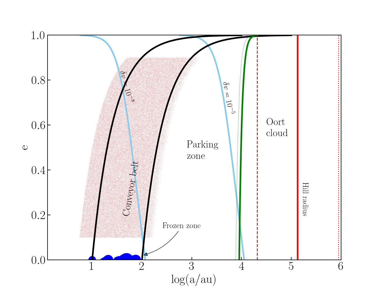
Figure 1: Orbital parameters of planets (blue bullets) and 141864 asteroids (red points) around the 200 nearest stars 1 Gyr ago. Here the right-most light blue curve gives the approximate inner edge of the Oort cloud using a mean local stellar mass of $\sim 1.0$ M_⊙  and a mean distance according to the Sun’s Hill radius in the Galatic potential ($\sim 0.65$ pc, red vertical line). The vertical dashed and dotted curves give the smallest and largest Hill radii experienced by any star throughout the simulations. The inner light-blue curve is given for a relative perturbation of $\delta v=10^{-8}$, the outer light-blue curve gives $\delta v=10^{-5}$. The green curve gives the distance from the host star for which the circularization time-scale of the Galactic tidal field is comparable to the eccentricity pumping time-scale of a test particle in the conveyor belt. The orbital configuration at today $1$ Gyr after the start of the simulation, is presented in figure 1. This figure is generated with the Python script plot_semimajor_axis_vs_eccentricity_of_planets_and_comets.py. This script, the required data, and the scripts to generate any of the figures in this manuscript including all required data are available through figshare (Portegies Zwart, 2020a). An animation of the simulation is available at https://youtu.be/0fYeAW3e9bQ.

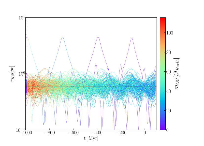
Figure 2: Approximate size of the Hill radius as a function of time for all the stars in the simulation since their birth until today and 100 Myr into the future. The mass of the Oort cloud is color coded (legend to the right). The star HD 103095 (see also figure 14) jumps out again with its curious orbit.

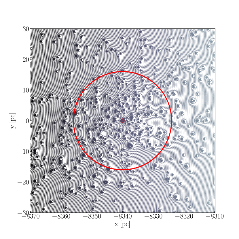
Figure 3: Equipotential surface of $\sim 795$ stars within 50 pc of the Sun projected on the xy-plane in the Galactic potential. To make the potential more visible, we magnified the stellar masses by a factor 300. The Sun is indicated with the red dot in the middle of the figure. The red circle, at $\sim 16$ pc indicates the inner region for which the analysis in this paper is performed. This volume contains the 200 nearest stars (Torres et al., 2019b). The script to generate this image, plot_nearby_stars_equipotential_surface.py, and the required data (filename gaia_nearby_stars.amuse), are both available at figshare (Portegies Zwart, 2020a).

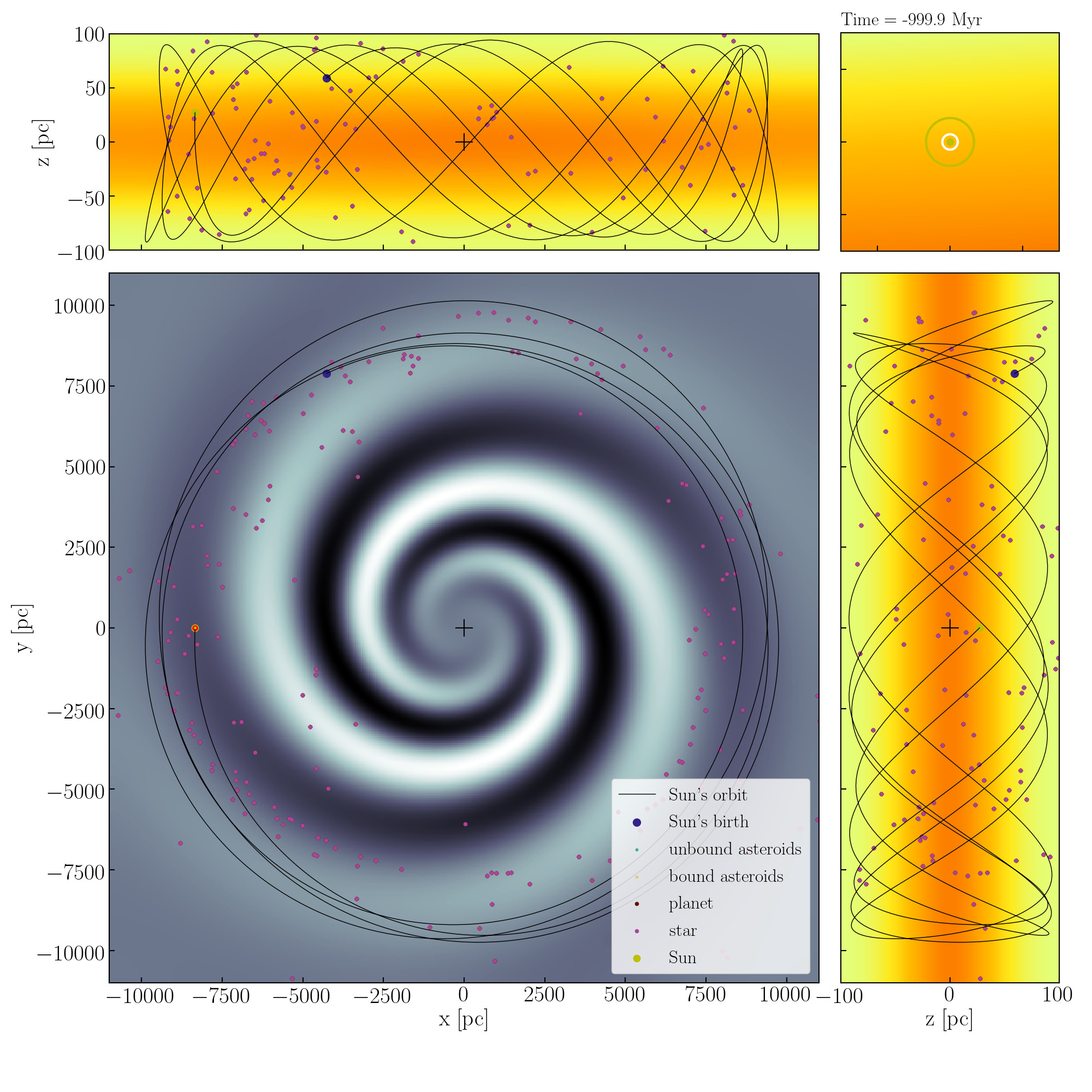
Figure 4: Positions of the 200 stars at their birth location in the potential of the Galactic 1.0 Gyr before the present. The solid curve shows the orbit of the Sun for the last Gyr. The colored background represents the adopted Galaxy potential: bottom left, top left, and bottom right views show the various Cartesian coordinates. The spiral structure is visible in the $X$-$Y$- plane (lower left), whereas the other two give panels only the edge-on views of the Galaxy is visible. The Sun’s starting position is indicated with the black bullet, it’s end position with a yellow bullet. The planets and asteroids of all the nearby stars overlay at this initial snapshot because the planetary systems are smaller than the symbol-size in the panels. The top-right corner-panel shows a magnified view of 6 by 6 parsec around the Sun. The outer circle shows the Hill radius at $\sim 0.65$ pc, the inner circle represents the inner edge of the Oort cloud at about $\sim 0.05$ pc. In this initial image, none of the stars are within 6 pc of the Solar system. The color graident in the top-right panel shows the local variation in the Galactic potential.

2.3.4 Initialization of planetary systems with asteroids

Once we have determined each star’s position and velocity a Gyr ago (see figure 4), planets, and asteroids are added. The planets are generated using the oligarchic growth model (Kokubo & Ida, 1998; Tremaine, 2015) using the implementation of Hansen & Murray (2013) We assumed the planets to form from a disk with 1 percent of the stellar mass with a minimum distance of 10 au from the host star, and adopting an outer disk radius of 100 au. The oligarchic growth model then leads to 3 or 4 giant planets, dependent on the disk’s mass.

In figure 5 we present for each star, the masses of the planets, and their distance to the host star. The inner-most planet is always initialized at 10 au, the other planets follow the oligarchic growth model, resulting in circular orbits in the same plane. The outer-most planet then arrives at $60$ to $76.3$ au (see figure 5). Planet masses range from $0.35$ M_Jupiter to $7.08$ M_Jupiter.

Several regimes are visible in figure 5. These result from the Oligarchic model in which planet masses increase with distance to the host star. Stars more massive than about 0.85 M_⊙  tend to acquire three relatively massive planets, whereas the lower mass stars receive four planets of somewhat lower mass. The cumulative distribution of the initial planet masses is presented in figure 6 (blue curve).

Once the planets are initialized, we add a population of asteroids as test particles in the planets’ plane. Each star receives 1000 minor bodies per 1 M_⊙  of the stellar mass. The pericenter distance was selected homogeneously between 5 au and 150 au with a random eccentricity between 0.1 and 0.9. This choice prevents asteroids to settle in resonances with the giant planets, where they continue to consume computer resources which is not the focus of this study.

The conditions for asteroids are presented in figure 1, where each red dot represents an asteroid. This choice of relatively high eccentricities may sound a bit odd for a debris disk, but it effectively places the asteroids in the planetary conveyor belt. In this parameter-space region, asteroids receive repeated gravitational kicks from the planets, driving them into wider and more eccentric orbits while preserving pericenter distance.

Before we start integrating each planetary system in the Galactic potential, the orbital plane is rotated to a random orientation (isotropically oriented in all fundamental angles). Each star with planets and asteroids then starts its orbit 1 Gyr ago at the calculated position in the Galaxy.

Each star with planets and asteroids are considered isolated with respect to the other stars. Since they are born throughout a wide area in the Galaxy (see figure 4) this assumption seems valid. Even today (when reaching the highest congregation) the stars are sufficiently far apart that the mutual influence of one star on the planetary system of another star is negligible. This is also illustrated in the top-right panel in figure 4, which shows today’s vicinity of the Sun.

While generating the planetary systems’ initial conditions, we ignore the binarity (or higher-order multiplicity) of some of the nearby stars. Several nearby stars are known to be multiple, and one of the important contributors to the local population of sōlī lapidēs, 61 Cyg A and B, actually is a binary system. We also ignored the known planets orbiting some of the catalog stars. This poses less of a limitation to the starting conditions because the known planets tend to have much tighter orbits than we adopted here, and they hardly provide constraints on the wider orbits. We leave the improvement of these assumptions for future work.

In figure 2 we show, an a function of time, as estimate for the Hill radius for each star in the simulation. At the earliest phase the Oort clouds are empty, which shows-up as the dark blue colors for all stars. But after some 100 Myr the respective Oort clouds start to be populated. As time progresses, these Oort clouds are depleted. The size of the Hill radius varies with the distance to the Galactic center. Near the Galactic center the Hill radius is small, whereas it grows when the star approaches apocenter in its orbit around the Galactic center. A smaller Hill radius, approaching perigalacticon, leads to enhanced mass loss from the Oort cloud.

To illustrate the orbits of the stars, we also present a projected view of the Galaxy with the orbits all stars in figure 7. Here we adopt the same color coding for the stellar orbits to make the comparison with figure 2.

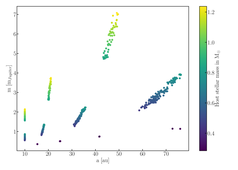
Figure 5: Initial planet mass as a function of the orbital separation around their parent star. The mass of the host star is color coded (see the color bar to the right). The two regimes, relatively low-mass ($\ {\raise-2.15277pt\hbox{$\buildrel<\over{\sim}$}}\ 0.85$ M_⊙) acquiring 4 planets according to the olycharcig growth model, whereas more massive stars only receive three planets.

Figure 6: Cumulative mass-distribution of the planets at the start of the simulation (blue) and at the current epoch ($1$ Gyr after the start of the simulations), in orange (for the bound planets) and green (for the unbound planets).

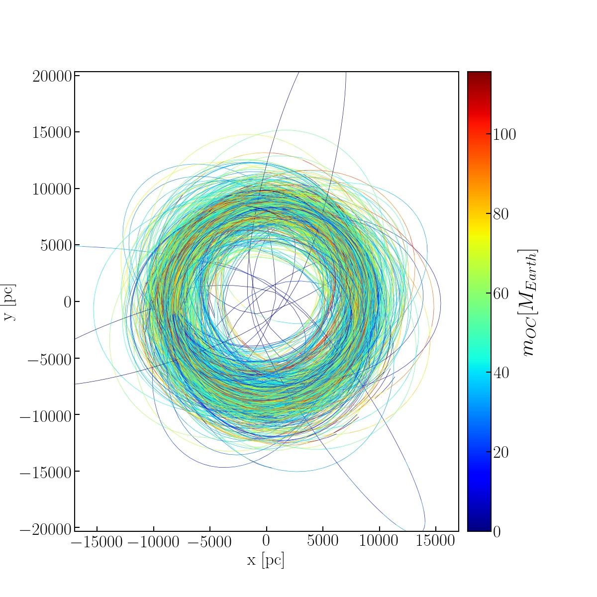
Figure 7: Mass of the Oort cloud for all the stars in the simulation since their birth until today and 100 Myr into the future. The legend, to the right, give the color coding in units of Earth masses. The star HD 103095 (see also figure 14) jumps out as having the most elliptical orbit.

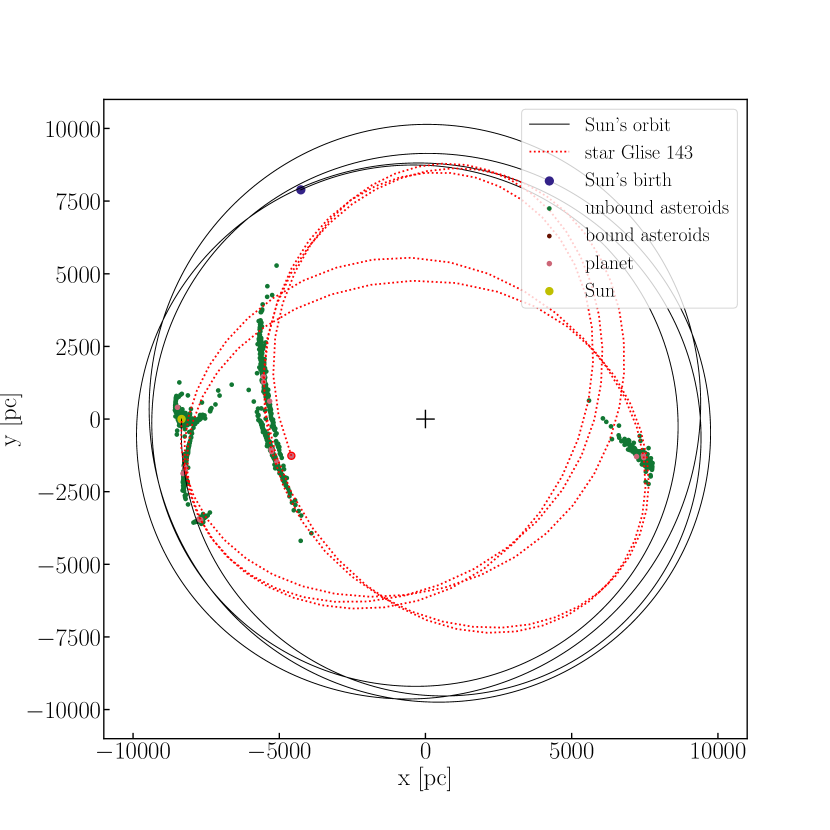
Figure 8: Examples of the Galactic orbits of Glise  143 (left panel) and the 61  Cyg binary (right). For Glise  143 and 61  Cyg  A we plot the position of the star and asteroids 1.0 Gyr ago, 0.8, 0.6, 0.4, 0.2 Gyr ago and today. We plotted the orbits of both stars 61  Cyg  A (red dotted line) and 61  Cyg  B (blue dotted line). Both stars start (1 Gyr) ago at the big bullet point to the top of the figure. The planets for 61 Cyg A are plotted only for the current epoch (when the star is near the Sun, to the left). At this time, two planets still orbit the star, but the other two planets were ejected early in the calculation. By the current time the ejected planets have moved away consideraby from the star. The main differences in the Galactic orbits of the two stars 61  Cyg  A and 61  Cyg  B (compare the red and blue dotted curves in the right-hand panel) is caused by the ejected of these two planets.

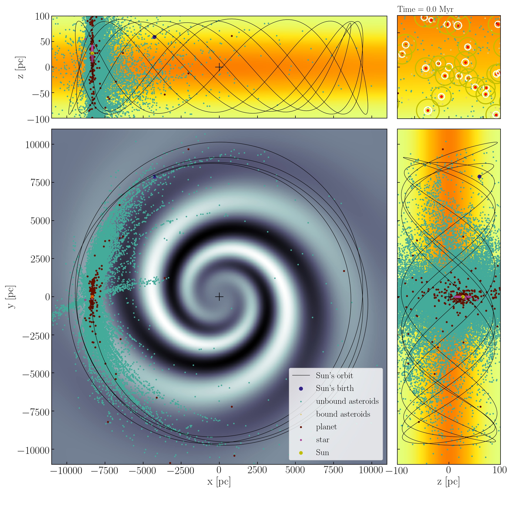
Figure 9: Current view of the Mikly way Galaxy along the three major projections and a close-up centered around the Sun in the top-right corner (as in figure 4. The orange, green, and red points indicate the bound and unbound asteroids and the planets, respectively. The stars are presented in bright red points. The Sun’s orbit in the Galactic potential is presented as the thin black curve which starts at the black bullet and ends at the yellow dot (to the left). For an animation, see https://youtu.be/0fYeAW3e9bQ.

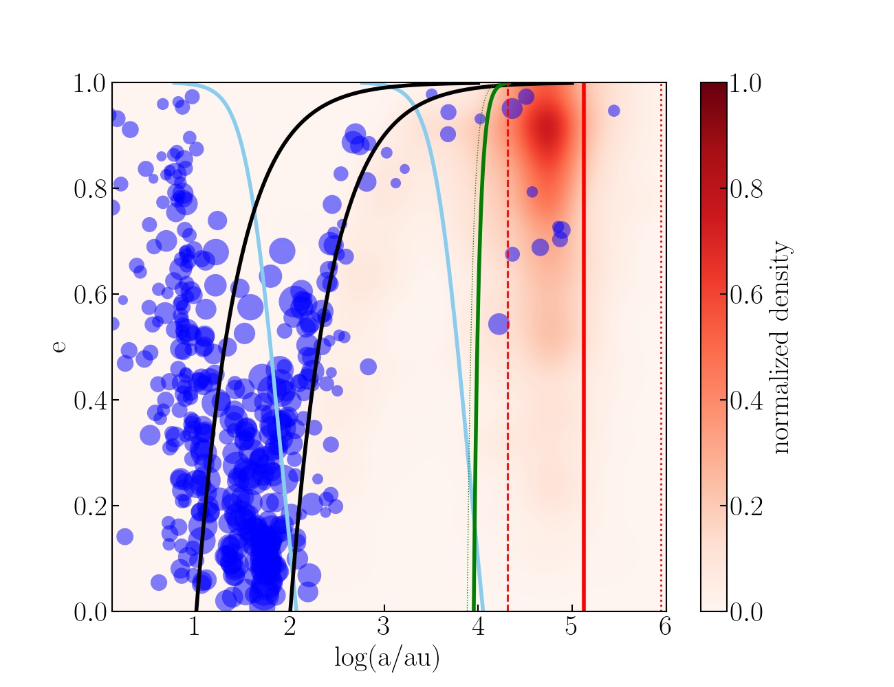
Figure 10: Orbital parameters of planets (blue bullets) and 141864 asteroids (red fuzz) at 1 Gyr after the start of the simulation. The various curves are described in figure 1. The size of the blue bullets is proportional to the mass of the planet. The two black curves indicate the pericenter distances associated with these mimimun and maximum initial orbital separations, indicating the limits of the conveyor belt. The minor bodies are presented as small red bullet points. In figure 10 we presented the initial conditions, and explained the terminology.

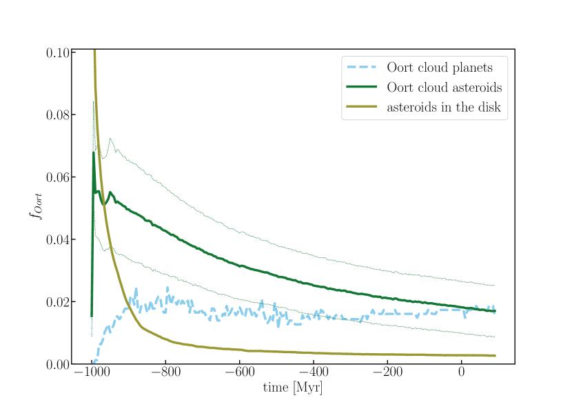
Figure 11: Evolution of the fraction of mass in a bound Oort cloud of their respective stars (solid green curve). The dotted curves give the dispersion (one standard deviation) among stars. The blue dashed curve gives the fraction of planets that populate the Oort cloud. The ocher-colored curve gives the fraction that remains in the disk either in resonant orbits or in the parking zone (outside the perturbing influence of the planets).

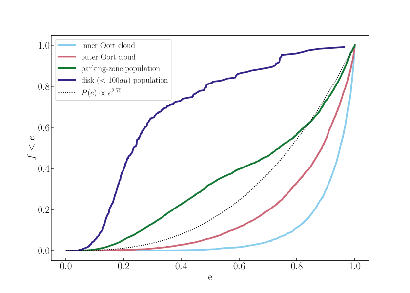
Figure 12: Cumulative distribution of the eccentricity in the inner and outer Oort cloud at an age of 50 Myr after the start of the simulations. The additional green curve gives the final distribution of $P(e)\propto e^{2.75}$. The simulated eccentricity distribution approach the theorectical curve in about 50 Myr.

2.3.5 Integrating the equations of motion

From the computed starting locations of the stars (see figure 4) and after planets and asteroids are situated around each (see figure 1), we integrate their positions (and those of the minor bodies) forwards in time for 1.1 Gyr. Asteroids, in this calculation feel the gravity of the star, the planets and the background potential of the Galaxy. The planets around a specific star feels their sibling planets, the parent star and the background potential. Each star feels its planets and the background galactic potential.

After 1 Gyr of integration all stars have arrived at (or at least near) the currently observed Gaia DR2 position. In figure 8 we show the back-and forwards calculation for two stars in our sample, Glise 143 and 61 Cygnus A. For the former, the back and forwards calculations, both remain within a line-width in the figure.

The yo-yo approach in a time-resolved smooth potential will result in precisely the same forwardly and backwardly orbital trajectory, as can be seen in the left panel of figure 8, where we demonstrate this for Glise  143. However, the forward calculations do not always precisely match the backward calculations because sometimes one or more planets are ejected while integrating the stellar orbit forwards in time. The result of a planet-ejecting system can be seen in the right panel of figure 8, where we integrated 61 Cyg A in the yo-yo approach. The forwards and backward calculation, in that case, result in slightly different orbits.

The ejection of a planet causes the center-of-mass of the star and planets to arrive at the anticipated Gaia DR2 location, but the forwardly calculated stellar trajectory will deviate from the backward calculation due to conservation of energy and linear momentum (in section 4 we discussion the consequences).

61 Cyg A is one of the worst cases in terms of the yo-yo approach, because two planets of $1.79M_{\rm Jupiter}$ and $0.72\,M_{\rm Jupiter}$ were ejected $\sim 105$ Myr after the start of the forward calculation. The massive planet is ejected first with a low relative velocity, but the lower-mass planet is ejected much more violently. This second planet is visible in figure 8, to the far right at a distance of about 7500 pc from the Galactic center (see also figure 9).

3 Results

In the yo-yo approach, each star reaches its current location after first being calculated backward in time and subsequently forwards (with minor bodies). The forward calculation is performed with planets and asteroids up to the current epoch and 100 Myr ’back to the future’. The current positions of the stars, planets and asteroids are presented in figure 9. During the calculations each planetary system is treated as isolated with respect to the other planetary systems.

Our calculations start with a star with planets and a conveyor belt filled with asteroids. The distributions in semi-major axis and eccentricity of planets and asteroids are presented in figure 1. While integrating forwards in time, the conveyor belt is emptied and the asteroids either remain bound or become unbound. In the next two sections, we discuss both, planets and asteroids bound to the parent star or unbound.

3.1 The population of bound planets and asteroids

We recognize several regions where an object can have a bound orbit around its parent star; it can be parked in the Kuiper belt or deposited in an Oort cloud. No asteroids are trapped in a resonant orbit with a giant planet.

3.1.1 Asteroids in the Kuiper belt and the Parking zone

In isolated planetary systems, as the ones simulated, the parking zone is expected to be deprived of asteroids. Still, $0.32\pm 0.01$ % of the asteroids in the simulations are deposited in their respective stars’ Parking zone. About one-third of these populate the area within 100 au along the conveyor belt’s outer edge. This population is visible in figure 10 as the red bullets between the right-most black solid curve and the right-most cyan curve. There is even an odd planet in the parking zone.

These parked asteroids are driven there through several scatterings with planets that have also migrated. Asteroids in the parking zone did not migrate along the conveyor-belt but were scattered several repeatedly by planets that themselves were scattered. As a consequence, the asteroid did not move along the conveyor belt but experiences a random walk until parked in a relatively wide ($100<a<10^{4}$ au) orbit with a relatively low eccentricity ($e\ {\raise-2.15277pt\hbox{$\buildrel<\over{\sim}$}}\ 0.8$). The right-most cyan curve in figure 10 indicates the outer edge of the parking zone (Portegies Zwart & Jílková, 2015) and the inner edge of the Oort cloud.

3.1.2 The formation and early evolution of the Oort cloud

Once an asteroid passes the right-most cyan curve in figure 10 we consider it member of the Oort cloud.

In figure 11 we present the evolution of the fraction of asteroids in the Oort cloud of their respective stars. In 25 Myr half the asteroids are removed from the planetary system. At the age of 100 Myr the fraction of asteroids in the disk dropped to $\sim 2$%, and after 1 Gyr, only 0.3 % of the asteroids still orbit in a disk within $\sim 100$ au around the parent star. All bound asteroids are eventually parked in some Kuiper belt, in the Parking zone or in the Oort cloud.

The Oort cloud builts up on a time scale of a few 100 Myr (see figure 2). At the age of 10 Myr, 4% to 6% of the original disk population has been launched into the Oort cloud. By that time, most orbits are still in the orbital plane of the planets.

In figure 10 we present the orbital distribution of asteroids that remain bound to their respective stars. The solid green curve indicates where the orbital period, $P_{\rm orb}$, equals the circularization-diffusion time-scale by the Galactic tidal field ($t_{\rm diff}$, Eq.5 of Duncan et al. (1987)). This line indicates the orbital parameters for which a particle tends to spend more time being perturbed by the Galactic tidal field (near apocenter) than by the Sun. The orbits of asteroids (and planets to this curve’s right, are circularized and isotropized by the Galactic tidal field. Asteroids between the right-most cyan and the green curves have difficulty being circularized by the Galactic tidal field; they tend to persist in rather high eccentricity orbits. However, if an asteroid is pushed further along the conveyor belt, deep into the Oort cloud, the Galactic tidal field’s circularization process operates on a time scale shorter than the time scale on which the planets eject asteroids. Asteroids that penetrate the Oort cloud further (to even wider but bount orbits) tend to circularize more quickly. The mean eccentricity in the Oort cloud is then a function of distance to the parent star and of time.

In figure 12 we present the cumulative distribution of the minor body’s eccentricities in the Oort cloud, 50 Myr after the start of the simulation. Here we make the distinction between an inner and an outer Oort cloud. This distinction is made at a perturbation factor of $\delta v=10^{-4}$. This corresponds to a semi-major axis of about $6\times 10^{4}$ au (for a circular orbit), compared to the division between the outer edge of the parking zone and the inner edge of the Oort cloud, which is at $\delta v=10^{-5}$ and corresponds to a semi-major axis of $\sim 10^{4}$ au (right-most cyan curve in figure 10).

In the first few tens of millions of years, when the Oort cloud is populated, the inner and outer Oort clouds have quite distinct distributions in eccentricity. This can be seen in the evolution of the mean eccentricity in these regions, presented in figure 13.

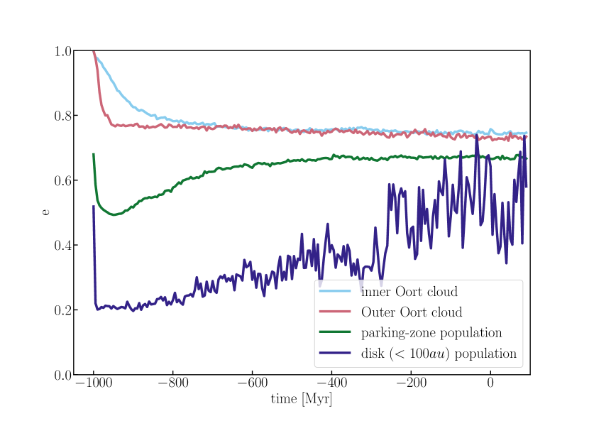
Figure 13: Mean eccentricity as a function of time for the Oort cloud (inner and outer) the asteroids in the parking zone and the disk (within 100 au). Initially, all asteroids have reativel high eccentricity, but this rapidly drops in the first few tens of Myr due to ejectsion by the planets. The Oort cloud population remains steady after about 100 Myr, whereas the more inner regions slowly converge to a similar eccentricity of $\sim 0.7$.

3.1.3 The evolution of the isotropic Oort cloud

After about 100 Myr both eccentricity distributions approach the thermal distribution. The Parking-zone population at this time is still converging to the thermal distribution. For a more thorough discussion on the asteroid migration in the Solar system, we refer to paper I (Portegies Zwart et al.  in preparation).

Once in the Oort cloud, the orbital distribution of asteroids becomes isotropic in inclination and their eccentricity drops from $\gg 0.9$ to a mean eccentricity of $\langle e\rangle\sim 0.7$ (see figure 13). 200 Myr after the start of the simulation, the Oort clouds are fully developed (see also figure 2).

After reaching a maximum, the number of asteroids in the Oort cloud starts to decay on a half-life time-scale of about 800 Myr. This time scale is considerably shorter than estimates for the Sun’s Oort cloud derived by Hanse et al. (2018). Our calculations accounted for the variations in the smooth Galactic potential through which the star moves, and part of the discrepancy stems from the wide range in the ellipticities of the Galactic orbits of nearby stars (see figures 8 and 2). The orbit of the Sun in the Galactic center, was also reason for Kaib et al. (2011) to discuss variations in the inner edge of the Oort cloud around the Sun. Our calculations (and those of Kaib et al., 2011) neglected the effect of passing stars, which tends to dramatically reduce the Oort cloud’s lifetime (Weissman, 1986; Stern, 1990; Matese & Whitman, 1992; Hanse et al., 2018).

3.1.4 The population of bound planets

Planets experience a similar fate as the asteroids, but it is much harder to eject a massive planet than a mass-less asteroid. Therefore, most planets remain bound to the parent star, and stay within the planetary region originally between 10 and 100 au. In figure 10 it is shown how the planets scatter along the curves of constant pericenter (flaring to the right) and constant apocenter (flaring to the left).

About $40$ % of the planets are ejected in the first 200 Myr. Eventually, after 1 Gyr, $\sim 24.8$ % of the planets remain bound to their respective stars, and $\sim 71.6$ % is ejected to become free-floating. Only $\sim 2$ % of the planets acquire a bound orbit in their star’s Oort cloud. The orbital distribution of these is isotropic in inclination with relatively low eccentricity ($\langle e\rangle\sim 0.7$, see figure 13). In figure 10, we present the orbital distribution of planets and asteroids that remain bound to their respective stars.

Planets in an Oort cloud are rare. In all our simulations, ten out of $\sim 736$ planets are parked in the Oort cloud. Only $\sim 5$ percent of the stars in our simulated solar neighborhood have a planet in the Oort cloud.

3.2 The population of unbound planets and asteroids

Most asteroids and planets do not remain bound to their host star. These objects become rogue planets and asteroids.

3.2.1 Rogue asteroids and sōlī lapidēs

The vast majority of asteroids become free-floating in the potential of the Galaxy. In figure 8 we present the evolution of the unbound asteroids for Glise 143 and 61 Cyg, an for HD 103095 in figure 14 along 5 (equally spaced) moments in time. At the start of the simulation, all asteroids (and planets) are bound to the star, but after 200 Myr most asteroids have already become unbound.

Although the fraction of bound asteroids is generally small (see figure 11), there are always some asteroids in the Oort cloud. Except for the halo star HD 103095 (Gaia DR2 4034171629042489088), which has lost all its asteroids at 100 Myr after the start of the simulation; No Oort cloud was formed around this star. The close perigalactic distance of this star together with the chaotic reorganization of its planets, resulting in the ejection of the lowest-mass planet ($\sim 1.59\,M_{\rm Jupiter}$), made it hard to preserve any objects bound to its Oort cloud. Its projected orbital trajectory is depicted in figure 14.

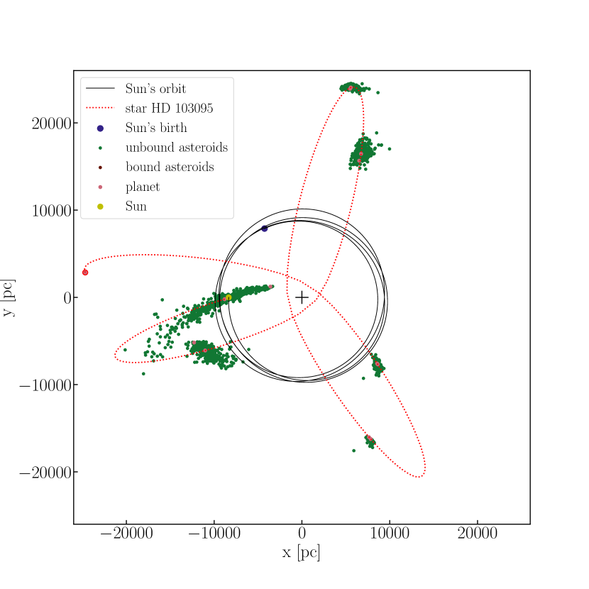
Figure 14: Projected Galactic orbit for HD 103095, which lost all its asteroids after the first passage of the Galactic center. HD 103095 (Groombridge 1830) is a is a metal-poor star ($\log(g)=4.71\pm 0.3$ and $[Fe/H]=-1.27\pm 0.2$ dex) Karovicova et al. (2018)) with a high proper-motion. According to Gaia DR2 its mass is $\sim 0.87$ M_⊙  (but only 0.66 M_⊙  according to Takeda et al. (2007)). In our calculations this star has a rather elongated orbit in the Galactic potential. Further description as in the legend of figure 8.

Escaping asteroid tends to hang around the parent stars (see also Correa-Otto & Calandra, 2019, who performed similar calculations for the Solar system). Much in the same way as tidal tails from star clusters tend to hang around along the trailing and leading orbital trajectory (Sandford et al., 2017). A similar structure is observed along the orbit of the Sagittarius dwarf (Majewski et al., 2003), Pal 5 (Odenkirchen et al., 2001) and other globular clusters (Piatti & Carballo-Bello, 2020). After the first $\sim 200$ Myr, there has been insufficient time, for the unbound asteroids to drift far away from the parent star, and the tidal asteroidal debris tails have a length of at most a few parsecs. After 600 Myr the debris tails have fully developed, extending over several kpc. The smearing and rotation of the debris tails is then determined by their orbital phase on the Galactic potential. For most of the orbit, the tidal tails closely follow the parent star’s orbit.

3.2.2 Rogue planets

The planetary systems in our simulations tend to be born in moderate stability, and some planets are ejected while interacting with each other or with the tidal field of the Galaxy. But this planet-ejection process is less common because of their large mass compared to the asteroids. Part of these planet ejections can be the result of numerical errors, because these systems are highy chaotic. The largest positive Lyapunov exponent indicates a stability time-scale considerably shorter than the time scale over which we integrate these systems. Although the adopted direct N-body code (Huayno) for integrating the planetary systems, there is some secular growth of the energy error, which in combination with the coupling to the Galactic potential may lead to spurious planet ejections.

A consequence of planet-planet scattering is the preferable ejection of lower mass planet, leaving the more massive planets in perturbed (possibly inclined and eccentric) orbits (Cai et al., 2018). This is illustrated in figure 6, where we present the initial mass-function of planets, the final mass-function (after 1 Gyr), and the mass function of the escaped planets. The final bound planet mass is larger than the initial planet mass, due to the relatively common escape of low-mass planets. Initially half the planets have a mass of $\sim 2.5\,M_{\rm Jupiter}$, whereas the mean mass of escaping planets is about $\sim 1\,M_{\rm Jupiter}$.

In our calculations, the effect of the Galactic tidal field on the dynamical evolution of the planets is small, except for those stars that have a small peri-galactic orbit (such as HD 103095). The strong perturbing effect of the Galactic center led Veras & Evans (2013) to argue that the Galactic-center region will have a higher proportion of rogue planets than the relative outskirts of the Solar neighborhood.

3.3 The current local Galactic distribution of asteroids

In figure 9 we present the distribution at the current epoch 1Gyr after the start of the simulation. It is no coincidence that at this moment, most objects are located around and near the Sun. Some structures along the Sun’s orbit in the Galactic potential and some streams perpendicular to the current Sun’s orbits are discernible. In the coming paragraphs, we further explore this population by presenting various slices in parameter space. The objective of this study is to better understand the local phase-space distribution of sōlī lapidēs.

3.3.1 Characterization of the local distribution of sōlī lapidēs

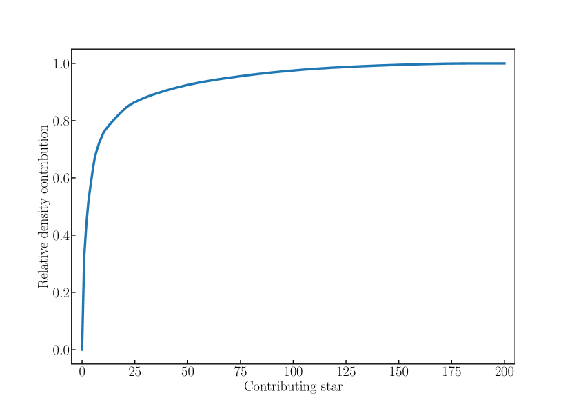
Figure 15: Relative cumulative contribution to the local density of minor bodies in the Solar neighborhood (sorted on their contribution to the local density of sōlī lapidēs). We used a KDE smoothing kernel with 1.41 pc.

In figure 15 we present the relative cumulative contribution of the local density of interstellar objects in the vicinity of the Solar system of the 200 nearby stars. In figure 16 the contribution for each individual star is sorted to its current (Gaia DR2) distance. The 10 most contributing stars to the local density of sōlī lapidēs  are painted red, all the others are blue.

The 10 most contributing stars are listed in table 1, and contribute more than 70% to the local density. About half the stars hardly contribute to the current local density of interstellar minor bodies. Even if the star is close to the Solar system, the stream of unbound asteroids may simply miss our current location in the Galaxy, as is the case for the second to fifth nearest stars to the Sun (see table 1), which contribute less than $\eta$ Cephei or Glise 143.

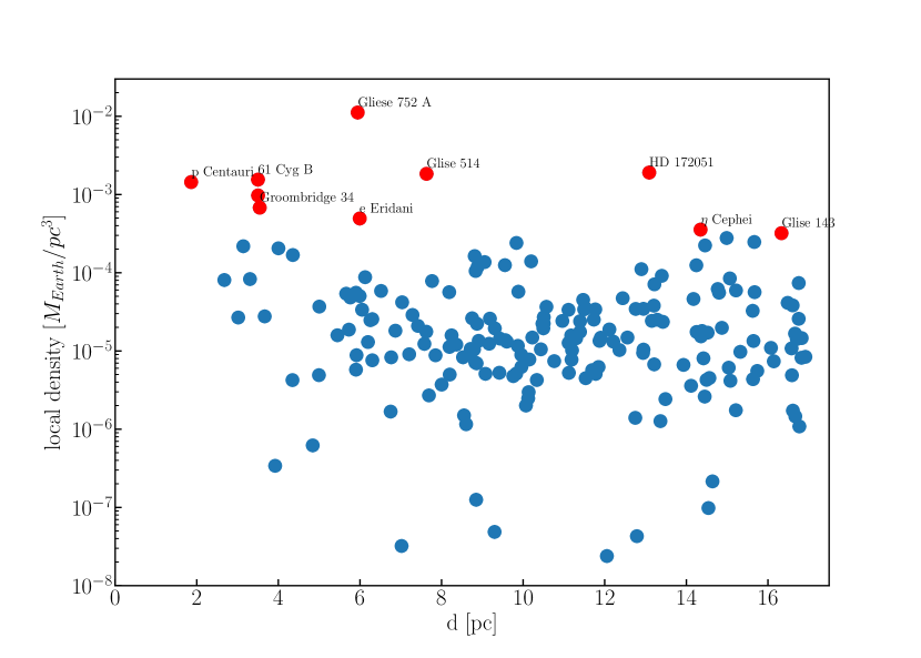
Figure 16: Individual contribution to the local density of sōlī lapidēs  calculated using a kernel density estimator with a smooting length of 0.39 pc. The ten biggest contributors to the local density are idicated in red and identified with their popular name.

The total local density of sōlī lapidēs  $\sim 0.027\,M_{\rm Earth}/$pc³. With an estimated mass for ’Oumuamua of $\sim 1.2\times 10^{9}$ kg (Portegies Zwart et al., 2018), the nearby stars contribute to the local density of interstellar asteroids by $\sim 1.2\times 10^{14}$ per cubic parsec.

The local density of interstellar minor bodies was estimated by Portegies Zwart et al. (2018); Do et al. (2018) to be of the order of $10^{15}$ objects per pc^-3. This density has contributions from evaporating Oort clouds or from the disruption of circumstellar debris disks. Both tends to be similar in scope in our analysis, because Oort cloud formation tend to be associated with debris-disk destruction (although more gently than the process discussed in Veras et al., 2011; Veras & Evans, 2013, who adopted that the disk would be obliterated by the post-asymptotic giant-branch evolution of the parent star).

It is hard to estimate how much stars further away contribute to the local density of sōlī lapidēs, in particular since we just demonstrated that far-away stars may contribute considerably when the Sun happens to move through the tidal-debris tail. We then estimate that Oort cloud evaporation and debris-disk distruction contribute $\ {\raise-2.15277pt\hbox{$\buildrel>\over{\sim}$}}\ 10$ % to the observed population of sōlī lapidēs.

To further illustrate this, the list in table 1 is sorted to the distance to the sun (n-dist $=1$ for the closest star p Centauri). Some nearby stars contribute considerably to the local density, but many major contributors are further away, as far as Glise 143 at about 16 pc. Note that the contribution to the local density depends somewhat on the adopted smoothing kernel for the density estimator. When we adopted a smoothing kernel of 1.0 pc instead of 0.38 pc, the star SZ UMa (the 70th nearest to the Sun) contributes almost as much to the local density of sōlī lapidēs  as 61 Cyg B.

Table 1: List of the 9 nearby stars that contribute most to the local (at the Solar system today) density of sōlī lapidēs. Listed are the Gaia DR2 identifier, the common name, the n-th closest star, the actual distance (in parsec) and velocity (in km/s) from the Solar system. In the 6th and 7th columns, we present the contribution to the local density of sōlī lapidēs  in number per pc^-3 and as a relative fraction. The last two columns give the mass of the star according to the most reliable estimates, according to the Gaia data archive,

Gaia DR2 id	name	n-dist	dist	v-rel	density		Gaia mass	mass
			[pc]	[km/s]	[pc-3]	relative	[M⊙]
4293318823182081408	Glise 752 A	23	5.94	54.1	0.0111	0.42	0.63	0.46
4079684229322231040	HD 172051	135	13.09	36.1	0.0019	0.07	1.07	1.0
3738099879558957952	Glise 514	44	7.63	57.9	0.0018	0.07	0.61	0.54
1872046574983497216	61 Gyc B	6	3.50	107.3	0.0015	0.06	0.64	0.63
4472832130942575872	p Centauri	1	1.86	142.6	0.0014	0.05	0.49	0.144
1872046574983507456	61 Gyc A	7	3.50	109.0	0.0010	0.04	0.66	0.70
385334230892516480	Groombridge 34	8	3.54	50.7	0.0008	0.03	0.58	0.38+0.15
4847957293277762560	$\epsilon$ Eridani	26	6.00	124.9	0.0005	0.02	1.01	0.85
2195115561163064960	$\eta$ Cephei	154	14.35	105.0	0.0004	0.01	0.74	1.6
4673947174316727040	Glise 143	185	16.33	68.0	0.0003	0.01	0.72	?

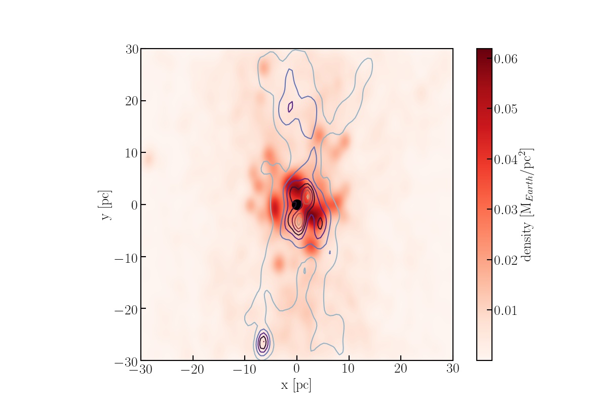
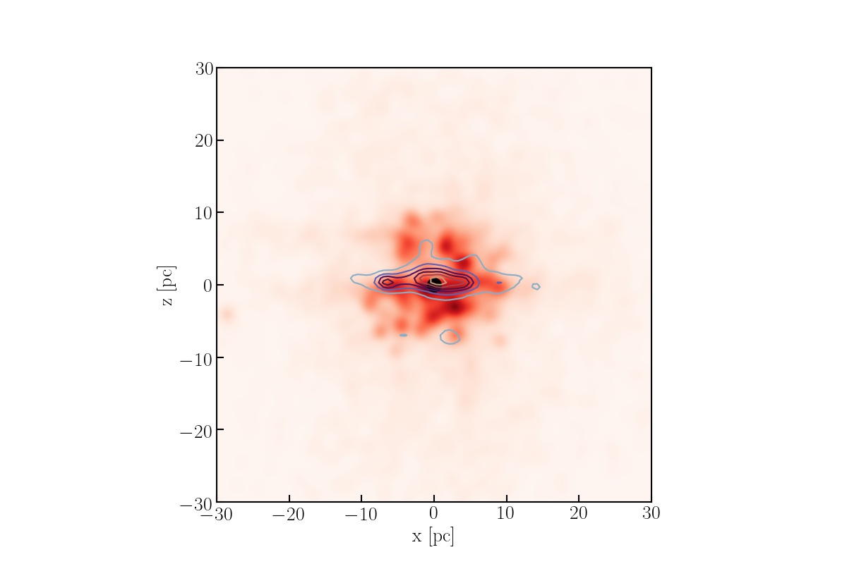
Figure 17: Local projected density of asteroids in the solar neighborhood (within 30 pc) in two projections: on the $X$-$Y$ plane for the upper panel is a projection in the galactic plane, whereas the bottom panel shows the $X$-$Z$ projection. Kernel-density smoothing kernel used was 0.104 pc. The red shades give the projected density of asteroids around the Sun. The contours give the local density only for the asteroids that originally orbited one of the ten stars in table 1.

In figure 17, we present the stars that contribute most prominently to the local minor-body density (see table 1) are presented as contours, whereas the others are indicated with a color-shaded kernel-density estimator. This distribution is clumpy, due to the minor bodies that escaped the gravitational pull of their parent stars with a relatively low velocity.

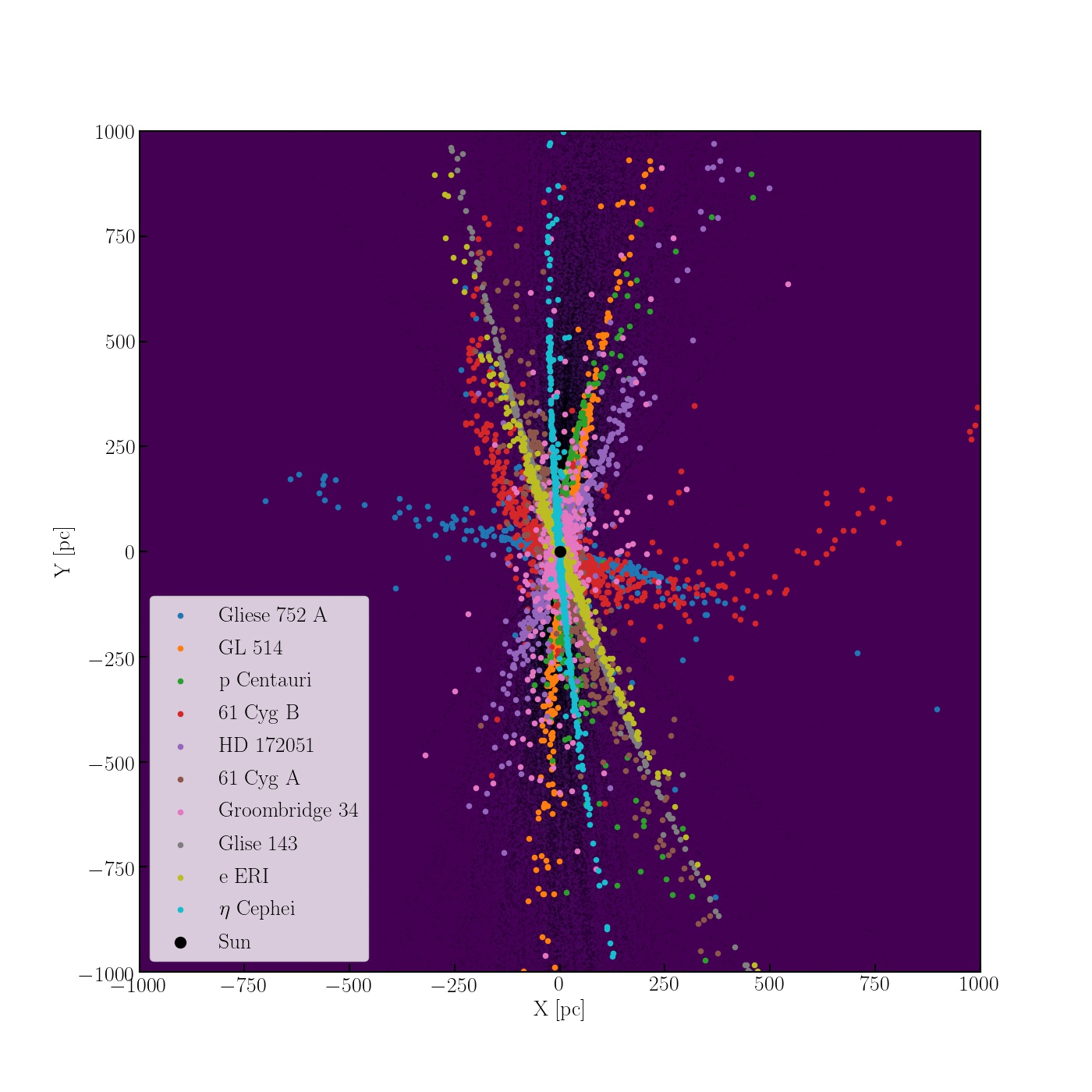
Figure 18: Current density of asteroids within 1 kpc of the Sun in the Galactic xy-plane and centered around the Sun (black bullet in the middle). The Galactic center is to the right. The 10 stars that contribute most to the local density of sōlī lapidēs  are indicated in colors (see legend), the others as small gray dots.

The debris streams are hardly visible in figure 17, because they tend to extend over a longer range and the relatively high local density causes the subtleties of the extended tails to wash away in the background. However, when we present the sōlī lapidēs  of the most contributing stars from table 1 on a larger scale the tidal debris streams become evident. This is illustrated in figure 18. Here the colored bullets identify the minor bodies of the 10 most important contributors. The Sun is in the origin because this is how the contributing stars were selected as nearest neighbors to the Sun (on which the picture was centered). The morphology and width of the streams depend on the orbit of the host star and orbital phase (see for example figure 8). A rather circular orbit around the Galactic center results in a narrow and elongated stream, as for the star $\epsilon$ Eridani, whereas a more elliptical orbit, such as for Glise 143, results in a broader distribution along its orbit. The interesting horseshoe shape of the tidal arms results from Glise 143 being close to apocenter in its orbit around the Galactic center: the trailing arm has the same spread as the leading arm but being located closer to the Galactic center it overtakes the leading arm.

3.3.2 The closest approaching objects

The majority of the Solar neighborhood stars experience their closest approach within a few hundred thousand years of the current epoch (see also Torres et al. (2019a)). The asteroids originally belonging to these stars swarm in front of– and behind them (as seen in figure 9). These tidal tails may cause asteroids to pass the Sun millions of years before or after the star has its closest approach to the Sun. We study this phenomenon to understand the extent to which other stars contribute to the local density of asteroids.

For this purpose, we analyze the same stars and minor bodies for the last 20 Myr and into the coming 20 Myr in the Galactic potential while keeping track of the closest approaches (the data is available in the data/NN directory in figshare). In this time frame, each asteroid has one closest encounter with the Sun. sōlī lapidēs  tend to arrive in families (as is also illustrated in figure 18). Each family originates from a single parent star. These families form from asteroids that escape the stellar gravity well, and continue in a similar orbit around the Galactic center as the parent star. A particular star can therefore lead to multiple close encounters with the Sun. These encounters may be spread out over the time-scale it takes the Sun to cross the tidal-debris tail, and this may be several Myr. During this time frame the Sun may have several encounters with different asteroids that originated from the same star. If several such interstellar asteroids were found, it would be much easier to find the source star.

In our simulations, the current dominant contributor to sōlī lapidēs  seems to be Glise 752. In reality, Glise 752 may not contribute any sōlī lapidēs  simply because, contrary to our assumptions, it may not have an Oort cloud. Glise 752, is a known binary system with a possible planet (Kaminski et al., 2018), but this does not make it necessarily a candidate responsible for the processes described here.

Figure 19: The moment of closest approach relative to the current epoch along the three major axes. Asteroids in the wake of the Solar system tend to have been encountered a while in the past, whereas those in front of we will have the closest encounter in the future.

Most asteroids from the current neighboring stars tend to have their closest approach with the Solar system in a rather short period of only a few Myr. Even those further away, or the high proper-motion halo-stars in the sample (see for example figure 14), tend to have their close approach within a few Myr of the current time. Since we selected the 200 nearest stars, this is not a surprise; it reflects how the current nearest stars were selected.

The majority of stars orbit the Galactic center in the same general direction as the Sun, but a few have retrogade orbits with respect to the Sun. They are visible in figure 19 as the green bullets among the blue bullets (and vice versa). These retrogade orbits can be identified in figure 20 as those with a large relative velocity with respect to the Sun.

Figure 20: Relative velocity at closest approach versus the distance of closest approach. The individual families of objects can be identified as individual spikes to short distance. To guide the eye we overplot the actual (unsmoothed) data with small dots.

The streams of asteroids in the left and right wings in figure 19, are the result of families of objects belonging to specific stars that pass today’s Solar system. Asteroids released around the stars’ leading tidal tail in the potential of the Galaxy have a close encounter with the Sun at an earlier epoch, whereas asteroids that escape through the trailing Lagrangian point have their closest approach to the Sun at a later time. These streamers are even more pronounced in figure 21 where we present the relative velocity at closest approach as a function of time of closest approach. Specific families of asteroids are now clearly visible, in particular at relatively low relative velocity.

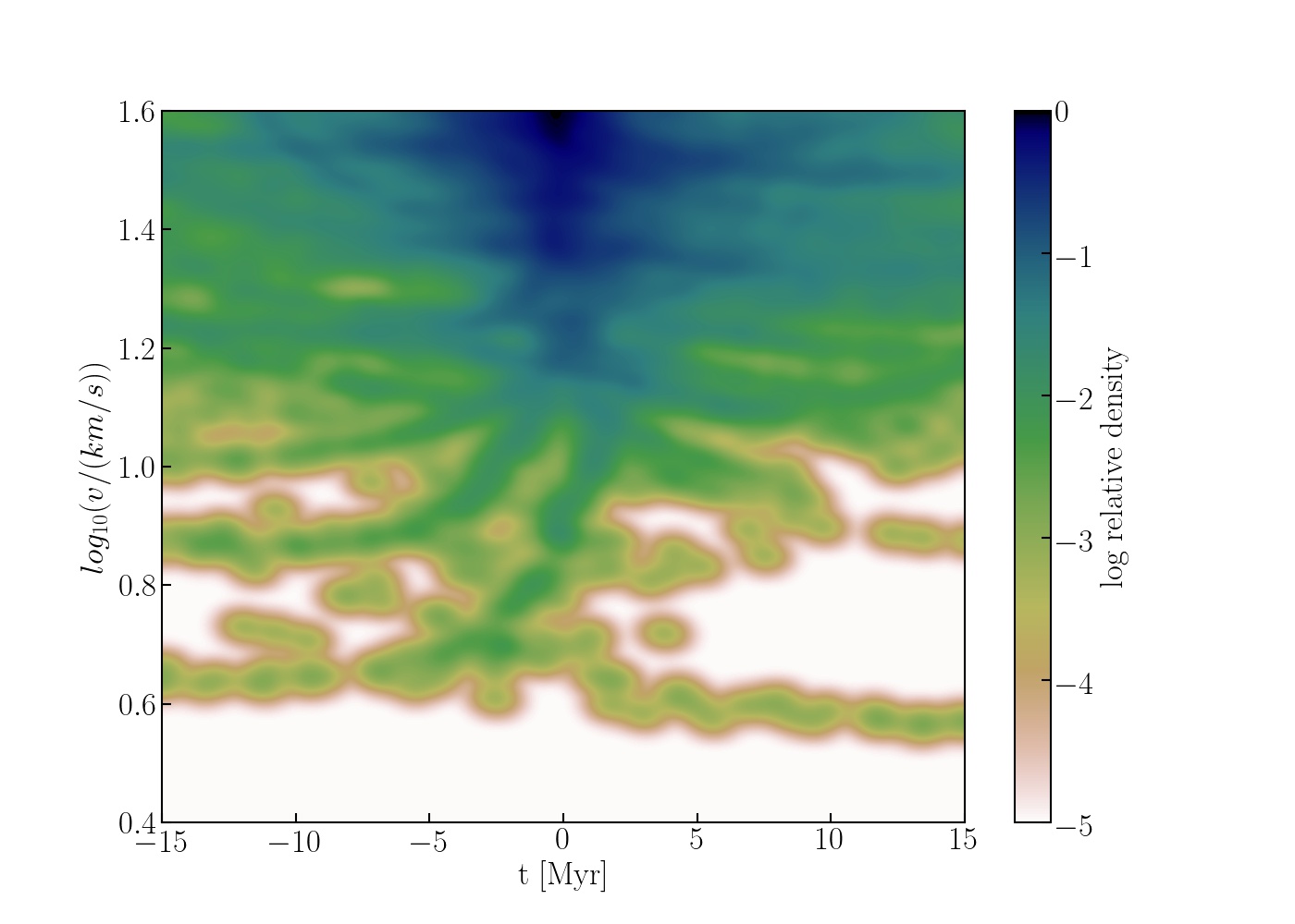
Figure 21: Distribution of relative velocity at the closest approach with the Sun as a function of moment of closest approach. The color colding gives density normalized to the maximum. The streams of objects with coherent motion in time represent families of asteroids belonging to a specific star.

In figure 22, we present the distance of the closest approach to the moment of closest approach. The concentration to the current epoch (at $t=0$ Myr) along the x-axis supports the results presented in figure 19 and 21. This result is consistent with earlier estimates of the distance and moment of closest approaching nearby stars (Bailer-Jones, 2015; Darma et al., 2019; Wysoczańska et al., 2020; Bobylev & Bajkova, 2020).

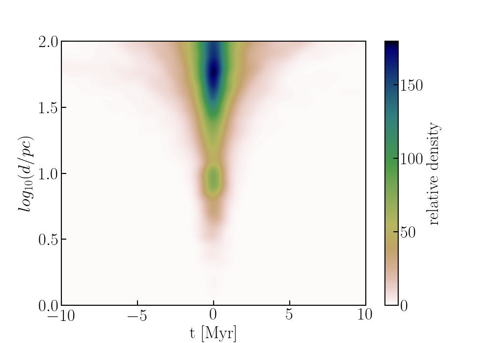
Figure 22: Distance of closest approach as a function of time since the current epoch. The color coding shows the relative density. the color coding is generated using a kernal-density estimator with a disperison of 1.41 pc.

When represented in encounter velocity relative to the Sun as a function of closest-approach distance, in figure 20, the various families are clearly visible to stay coherent. At the resolution of the simulations, however, the closest approach distance to a particular asteroid that originates from a particular star is merely a result of shot-noise due to our relatively low resolution of 1000 asteroids per M_⊙.

3.3.3 Closest free-floating planets

In figure 23, we present the time of closest approach and its distance for the planets in our simulations. Whereas asteroids tend to be spread out over a much large phase-space volume, planets are confined to the current epoch within about 10 pc. Massive planets stay close to their parent stars. Although some are eventually ejected to become rogue planets, the ejection velocity is so low that they stick around even more prominently than the asteroids. Asteroids show a similar over-density, as can be seen in figure 22, but the population is less pronounced due to the large number of sōlī lapidēs  at a larger distance and the small number of asteroids that remain bound to their parent stars.

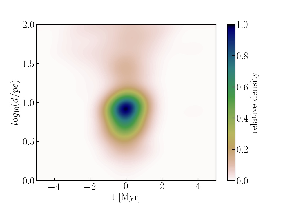
Figure 23: Distance of closest approach as a function of time since the current epoch. The color coding shows the relative density. The color coding is generated using a kernal-density estimator (KDE) with a disperison of 1.41 pc.

The relative proximity of free-floating planet to their parent star is also visible in figure 9, here planets are more closely surrounding the current Solar position in the Milky-way Galaxy in comparison to the asteroids.

4 Discussion

We have simulated a hypothetical population of asteroids and planets in orbit around the 200 nearest stars to the Sun. In this calculation we ignored all known planets and binary systems among this population, but treated each star as single, orbiting in a semi-analytic potential of the Milkyway Galaxy. Our calculations start 1 Gyr ago, by calculating the positions and velocities of the 200 nearby stars backward with time to this epoch. From there, we surround each star with 3 or 4 giant planets in circular orbits between 10 au and 100 au, and 1000 minor bodies per M_⊙  in the conveyor belt (with pericenter between 5 au and 150 au).

4.1 Time reversibility and the uniqueness of the calculation

The integration is continued from 1 Gyr ago and to 100 Myr into the future. This backwards-forwards yo-yo approach is time reversible and the star, after calculating back to the future, arrives at precisely the same location with the same velocity as where it is observed today.

In our simulations, however, the simulated positions and velocities of individual stars today do not always match the observations by Gaia DR2, because some of the stars lose one or more planets on the way, causing its orbit to deviate from the calculated orbit as discussed in section 2.3.3. The median of the relative difference in a position perpendicular to the orbit of the star (given the current solar position this is along the Galactic x-axis) is only $0.39$ au, but along the orbit, the discrepancy is $96.7$ au in the y-direction, and $451.7$ au in the galactic z-direction. There are a few cases, however, for which the ejection of a planet leads to a considerable deviation of the parent stars’ orbit in comparison to the adopted orbit when calculated without planets. One example is visible in figure 9 to the left of the location of today’s Solar system. This star, 61 Cyg A, has an orbit in the Galactic potential which makes a relatively large angle to the current Solar motion. Since the dispersion in the orbital calculation (due to possible ejected planets) is largest along the orbit, this star is now located rather far from its anticipated location according to the Gaia data. Also for other stars, the discrepancy between the center-of-mass and the actual stellar orbit is largest along the orbit.

4.2 The 1 Gyr time window

For the yo-yo approach, we choose a fixed time frame for the calculations of 1 Gyr. Ideally, we should have followed each star since its birth in the Galactic potential to the current time. This procedure would be hindered by our lack of knowing the ages of all nearby stars and the long-term evolution of the potential of the Milky way Galaxy. Another complication arises from the uncertainty in the actual planet population and the presence of a debris disk. To achieve a consistent assessment of the potential contribution to the observability of the tidal asteroid-tails of these stars would then require many calculation for each star (to integrate over the uncertainty in the kinematics and the orientation of the disk) and run these simulations with a potential model that matches the history of the Galaxy.

The first analysis would be expensive in terms of computer time, but not impossible. We simply lack the knowledge of the stellar ages and do not know the history of the Galaxy well enough to perform such a simulation.

The tidal tails develop in the first 100 Myr, and then slowly diffuse, causing the debris trail to grow in length. This later diffusion process is slow and develops on a Gyr time scale. For the length of the tidal-debris tails of the nearest 200 stars, the star’s ages are not critical. This would be different if a particular star is younger than about 200 Myr, in which case the star’s Oort cloud would still be in development, and the tidal tail has not yet fully formed.

4.3 The erosion of the Oort cloud

According to calculations on the evolution of the Sun’s Oort cloud, Hanse et al. (2018) derive a half-life of $t_{{1\over 2}OC}=3$ to $10$ Gyr. This range stems from studying figure 4 of Hanse et al. (2018) where erosion proceeds faster due to close encounters with other stars Duncan et al. (2011).

Far-away encounters are not very important for the erosion of the Oort cloud, but the occasional close encounter induces a major degradation of the Oort-cloud population. Without those close encounters, they estimated the Oort cloud half life to be of the order of $t_{{1\over 2}OC}=8$ to $10$ Gyr, which is an order of magnitude longer than the our estimate of $t_{{1\over 2}OC}\simeq 800$ Myr.

Part of the discrepancy can be understood from the lower stellar masses in our calculations, which measures $\langle m\rangle=0.72\pm 0.21$ M_⊙. As a result, the Hill radius of the typical nearby star is smaller than that of the Sun. It will be harder for these stars to keep asteroids bound. This effect leads to an increase in the evaporation rate, but cannot explain the order of magnitude difference.

Another argument for our smaller Oort-cloud lifetime stems from the orbits of many of the stars, which have somewhat larger ellipticities than the Sun’s orbit around the Galactic center (see figure 7). This leads to a strongly varying Hill radius (see figure 2), a consequential stronger perturbation by the Galactic tidal field, which leads to the easier ejection of asteroids (De Biasi et al., 2015). We already demonstrated this process to be responsible for the evaporation of the Oort cloud of Glise 752 in section 3.3.2. On average, this process reduces the Oort-cloud lifetime but is still insufficient to explain the discrepancy with Hanse et al. (2018).

We argue that the most important difference between the derived lifetime of the Oort cloud by Hanse et al. (2018) and our study stems from how we form the Oort cloud from a population of asteroids in the conveyor belt, rather than initializing them with a smoothed and virialized distribution function, as was done in Hanse et al. (2018). The latter method results in a more stable Oort cloud and a lower evaporation rate.

With our derived half-life on the Oort cloud of $\sim 800$ Myr, and a current mass of the Oort cloud of $2$ – $40$ M_Earth (or $10^{10}$ to $10^{12}$ asteroids, Weissman, 1996), we derive an initial mass of the Oort cloud of $3.2$ – $64$ M_Jupiter. Which, with an Oort cloud retention fraction of $\sim 0.06$, results in an initial debris disk of $0.003$ M_⊙  and 0.064 M_⊙. This value is consistent with the initial value of 0.01 M_⊙  which we adopted in our simulations. These numbers are consistent with earlier estimates on the mass of the Oort cloud (Weissman, 1983; Marochnik et al., 1988; Dones et al., 2004).

Although ignored in our calculations, occasional close passages of stars turn out to be important for the Oort cloud’s erosion. Therefore, these passing stars are also expected to be important for the extent and morphology of the debris streams of sōlī lapidēs. We ignored this effect in our calculations, and it is hard to anticipate this effect, except maybe in a statistical sense.

4.4 Interstellar visitors: ’Omuamua and Borisov

One of the objectives of this study is to obtain a better understanding of the contribution of nearby stars to possible interstellar visitors, such as 1I/’Oumuamua and 2I/Borisov. It was anticipated that these objects may have originated in the Oort cloud of other stars (Moro-Martín, 2019).

In an attempt to find the origin of ’Oumuamua and Borisov, Dybczyński & Królikowska (2018) studied the stars within 60 pc (using Gaia DR2 data) but conclude that it would be difficult to find a stellar origin of the two sōlī lapidēs. The accuracy of the orbits of ’Oumuamua and Borisov, and the scattering in the Galactic disk make it hard to trace back their origin beyond some $15$ pc or within the last $10$ Myr (Hallatt & Wiegert, 2020).

Despite this earlier analysis, in which nearby stars were excluded as the source of the two observed sōlī lapidēs  (Portegies Zwart et al., 2018; Bailer-Jones et al., 2018, 2020), Dybczyński & Królikowska (2018) argued that Gl 876 might be a suitable host of ’Oumuamua. Currently, Glise 876 is at a distance of 4.68 pc, but 0.817 Myr ago it had the closest approach to the Sun at a distance of 2.24 pc. Glise 876 (Gaia DR2 2603090003484152064) regretfully, was not part of our analysis. If indeed Glise 876 is a contributor to interstellar visiting rocks or icy bodies, we might expect multiple objects to come from the same source.

Objects such as ’Oumuamua and Borisov, enter the solar system on unbound orbits and leave again after interacting with the Sun. Both objects are represented with bullet points in figure 24, which indicates their point on the sky from which they appeared to be coming, calculated for ’Oumuamua by Bailer-Jones et al. (2018) and for Borisov by Bailer-Jones et al. (2020).

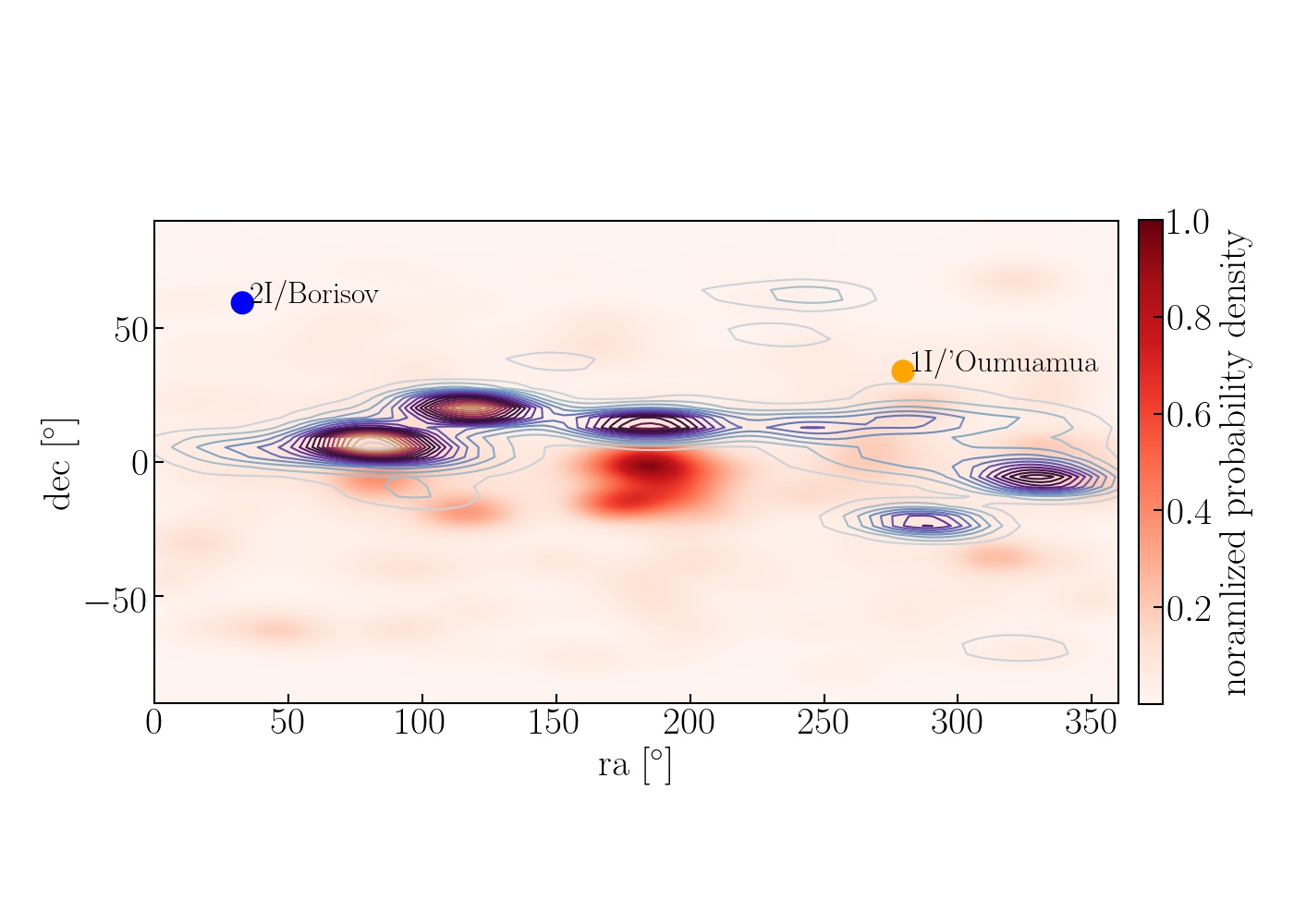
Figure 24: Sky projection of nearby asteroids. The blue and orange bullet points indicates the direction from which Borisov and ’Omuamua entered the Solar system from the analysis of Bailer-Jones et al. (2018) and Bailer-Jones et al. (2020), respectively. The color coding gives the relative contribution to the local density, wheras the contours give the same information for the 9  nearest stars in table 1.

Overplotted in figure 24 is the distribution of all minor bodies in our calculations (red shaded region) and of the stars that contributed the most to nearby objects from table 1 (contours). Borisov is quite far from these distributions, but ’Oumuamua is approximately near some of the asteroids that originated from relatively nearby stars.

If multiple objects originate from the same stellar source, they do not necessarily come from the same direction or with a similar velocity. If we could argue that multiple intruders have a similar origin, it may be possible to identify the family and the star from which they originated. This was illustrated in figure 19, where we presented contributing streams of the most contributing stars.

The time ’Oumuamua has been floating around freely in space was estimated to be less than a Gyr (Portegies Zwart et al., 2018; Hands et al., 2019; Hallatt & Wiegert, 2020). In our calculations, tidal tails remain coherent for considerably longer. It is then conceivable that ’Oumuamua is still a member of the leading or trailing arm of debris around its parent star. In that case, we might expect more objects entering the solar system from the same Galactic direction.

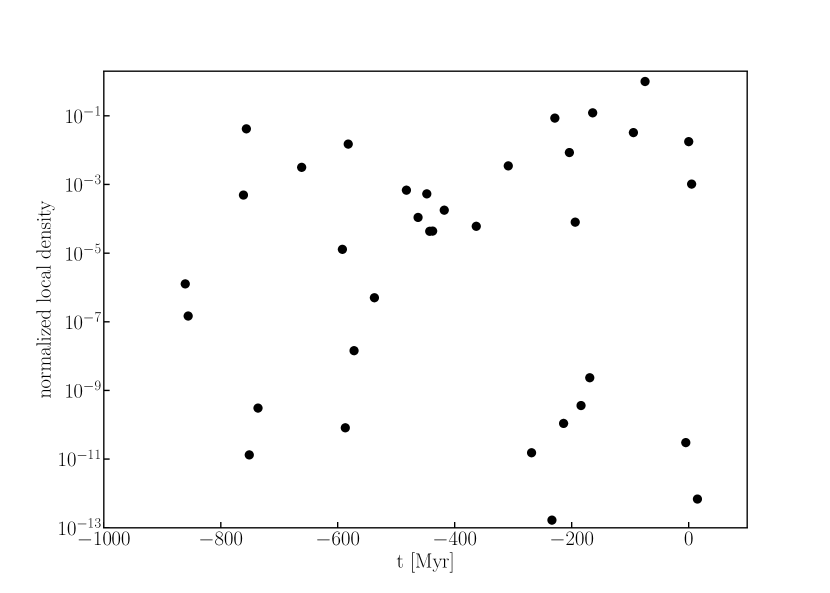
Figure 25: Evolution of $\log_{10}$ density of interstellar asteroids in the Solar vicinity. Calculations were performed with a KDE smoothing kernel with a kernel bandwidth of 1.4 pc. Both curves are normalized to the same maximum of $\sim 0.027$ M_Earth/pc³ at today’s epoch. The adopted a KDE smooting kernel of 1 pc³.

To further verify that the nearby stars contribute prominently, but that far away stars may still contribute considerably, we present in figure 25 the evolution of the local (and maximum) density of sōlī lapidēs. Today (at $t=0$ Myr) the peak reached is about two orders of magnitude higher than at any other moment. Narrow peaks in time appear when the Solar system happens to move through the debris-stream of another star.

Today’s high peak in the local density of sōlī lapidēs  does not mean that we live at a special time, but it is merely a consequence of our initial selection of the 200 nearby stars. At any time, there will be some stars through which’s stream we move, giving rise an enhanced encounter rate with the asteroids in its tidal streams. To what degree this results in a continuous encounter rate or in rather discrete peaks is at this point hard to assess. Based on our simulations, we cannot determine the temporal variations in this encounter rate because this depends on the extend and density tructure of the individual streams. The resolution of our caluclations ware insufficient to determine this structure, and it would require us to take many more nearby (and further away) stars into account in the analysis.

5 Conclusions

We have studied the possible evolution of the population of today’s 200 nearest stars from the Gaia DR2 catalog in the Galactic potential including a hypothetical population of initially bound planets and asteroids. The objective was to characterize the local environment of the left-overs of the planetary scattering process around these stars in order to constrain the distribution of asteroids and free-floating planets in the Sun’s vicinity. We ignore the contribution of other stars, not near to the Sun. Our assumptions on the initial conditions are somewhat capricious because we do not know if these stars have debris disks.

For the initial conditions, we assume each star to be born a billion years ago with 3 or 4 planets in circular orbits between 10 and 100 au. The planet masses range from 1 to 7 times the mass of Jupiter. Each planetary system is further populated with 1000 point-mass asteroids per M_⊙  in the plane of the planets. The orbits have a pericenter distance between 5 au and 150 au, and eccentricities randomly between 0.1 and 0.9. Therefore, they could be viewed as an excited population that already underwent some scattering from the planets formation process and early dynamical evolution. Each planetary system is oriented randomly. The birth location for each star is determined from back-calculating its orbit in the Galactic potential.

After setting up the initial conditions, we numerically integrate all the stars, planets, and asteroids in the Galactic potential for 1.1 billion years, until the current epoch and 100 Myr into the future. While performing these calculations, we keep track of the positions of the Sun and all other objects to find the moment of closest approach between any object with respect to the Sun.

We find that in the 1 billion years of evolution, 98 percent of the asteroids become unbound and turn into free-floating asteroids, or sōlī lapidēs. About 2 percent of the asteroids remain bound to their parent star in the form of an Oort cloud, and $\sim 0.31$ percent remains bound to the parent star in stable orbits outside the range of influence of the outer-most planet, in the parking zone. A tiny fraction of asteroids, $\sim 0.1$ % (164) find themselves bound to the parent star outside their respective Hill radii.

The fraction of planets that remain bound in the parent star’s Oort cloud is $\sim 2$ %, similar to the fraction of asteroids that remain bound. This fraction is consistent to the results of the calculations by Correa-Otto & Calandra (2019).

In the first few tens of millions of years, when the Oort clouds are filled, the inner and outer Oort clouds have quite distinct distributions in eccentricity. This changes after about 50 Myr, when the eccentricity distribution approaches the thermal distribution, as demonstrated in figure 12.

The distribution in eccentricities of the Oort cloud objects reaches a steady-state of $P(e)\propto e^{2.75}$ after about 50 Myr. The distribution in semi-major axes is flat in $\log$ from $10^{4}$ au to $10^{5}$ au. The half-life of the Oort clouds in our calculations is 800 Myr, which is considerably shorter than found in earlier studies. The short Oort cloud half-life in our simulation is attirbuted to the correlation between semi-major axis, eccentricity, and inclination. But some contribution also comes from the lower masses of the stars and their relatively high eccentricity in the Galactic potential.

The $10$ stars in the Gaia DR2 database that contribute most prominently to the probability of producing an interloper are not necessarily the closest stars. Some relatively distant stars contribute more prominently than some closer in. This probability depends on the orbit of the particular star (and its asteroids) with respect to the Sun. A star that orbits parallel to the Sun in the Galactic potential is unlikely to contribute to the local density of sōlī lapidēs  whereas a crossing orbit results in a local overdensity. A relatively far away star can then still contribute considerably to the local asteroid density, in contrast to a more local star. These peaks in over-density of local sōlī lapidēs  does not have to coincide with the closest approach for that particular host star, but it may happen millions of years earlier or later.

The contribution to the locally observed population of sōlī lapidēs  strongly depends on whether or not the Sun happens to move through the tidal asteroid-tail of another star. Some of these trails are dense and narrow, and may give rise to a local enhancement in the incident rate of interstellar objects interacting with the Solar system. We derive a current local density of sōlī lapidēs  from the 200 nearest stars of $\sim 0.027\,M_{\rm Earth}/$pc³. With a typical mass comparable to ’Oumuamua, we then arrive at a local number-density of $\sim 1.2\times 10^{14}$ per cubic parsec, which is a factor of 10 lower than earlier estimates based on the two known sōlī lapidēs. We, therefore, argue that the nearest few hundred stars contribute to the rate of interstellar asteroids visiting the Solar system, but they are probably not the dominante source.

We expect considerable structure in the distribution of interstellar asteroids. If observable, this structure will inform us about the Galactic potential, the orbits and ages of the nearby stars and the internal reorganizations their planetary systems might have endured. On these grounds, we do expect considerable temporal variations in the encounter rate of sōlī lapidēs.

5.1 Energy consumption of this calculation

The evolution of each star (incuding the planets, asteroids and the Galactic tidal field) was computed in 3 to 7 days on a one GPU and 6 cores. The total computer time spend summs up to about 1000 hours on GPU and 6000 CPU hours. With 180 Watt/h per GPU and 12 Watt/h per CPU our total energy consumption for the calculations is about 250 kWh. With $0.283$ kWh/kg (Wittmann et al., 2013) results in 200 tonnes Co₂, quite comparable to launching a rocket into space (Portegies Zwart, 2020b).

Public data

The source code, input files, simulation data and data processing scripts for this manuscript are available at figshare under DOI 10.6084/m9.figshare.12834803.

An animation of the simulation is presented in https://youtu.be/0fYeAW3e9bQ.

References

- Abolfathi et al. (2018) Abolfathi, B., Aguado, D. S., Aguilar, G., et al. 2018, ApJS, 235, 42
- Anderson & Francis (2012) Anderson, E. & Francis, C. 2012, Astronomy Letters, 38, 331
- Andrae et al. (2018) Andrae, R., Fouesneau, M., Creevey, O., et al. 2018, A&A, 616, A8
- Bacci et al. (2017) Bacci, P., Maestripieri, M., Tesi, L., et al. 2017, Minor Planet Electronic Circulars, 2017-U181
- Bailer-Jones (2015) Bailer-Jones, C. A. L. 2015, A&A, 575, A35
- Bailer-Jones et al. (2018) Bailer-Jones, C. A. L., Farnocchia, D., Meech, K. J., et al. 2018, AJ, 156, 205
- Bailer-Jones et al. (2020) Bailer-Jones, C. A. L., Farnocchia, D., Ye, Q., Meech, K. J., & Micheli, M. 2020, A&A, 634, A14
- Belleman et al. (2014) Belleman, R., Bédorf, J., & Portegies Zwart, S. F. 2014, Kirin: N-body simulation library for GPUs, astrophysics Source Code Library
- Bobylev & Bajkova (2020) Bobylev, V. V. & Bajkova, A. T. 2020, Astronomy Letters, 46, 245
- Borisov (2019) Borisov, G. 2019, in (Minor Planet Electronic Circular No. 2019-R106), 11
- Brasser & Morbidelli (2013) Brasser, R. & Morbidelli, A. 2013, Icarus, 225, 40
- Buder et al. (2018) Buder, S., Asplund, M., Duong, L., et al. 2018, MNRAS, 478, 4513
- Cai et al. (2018) Cai, M. X., Portegies Zwart, S., & van Elteren, A. 2018, MNRAS, 474, 5114
- Correa-Otto & Calandra (2019) Correa-Otto, J. A. & Calandra, M. F. 2019, MNRAS, 490, 2495
- Darma et al. (2019) Darma, R., Hidayat, W., & Arifyanto, M. I. 2019, in Journal of Physics Conference Series, Vol. 1245, Journal of Physics Conference Series, 012028
- De Biasi et al. (2015) De Biasi, A., Secco, L., Masi, M., & Casotto, S. 2015, A&A, 574, A98
- Do et al. (2018) Do, A., Tucker, M. A., & Tonry, J. 2018, ApJ, 855, L10
- Dones et al. (2004) Dones, L., Weissman, P. R., Levison, H. F., & Duncan, M. J. 2004, Oort cloud formation and dynamics, ed. M. C. Festou, H. U. Keller, & H. A. Weaver, 153
- Duncan et al. (1987) Duncan, M., Quinn, T., & Tremaine, S. 1987, AJ, 94, 1330
- Duncan et al. (2011) Duncan, M. J., Babcock, C., Kaib, N., & Levison, H. 2011, in AAS/Division of Dynamical Astronomy Meeting #42, AAS/Division of Dynamical Astronomy Meeting, 9.03
- Dybczyński & Królikowska (2018) Dybczyński, P. A. & Królikowska, M. 2018, A&A, 610, L11
- Edgeworth (1943) Edgeworth, K. E. 1943, Journal of the British Astronomical Association, 53, 181
- Feng & Jones (2018) Feng, F. & Jones, H. R. A. 2018, ApJ, 852, L27
- Froncisz et al. (2020) Froncisz, M., Brown, P., & Weryk, R. J. 2020, Planet. Space Sci., 190, 104980
- Fujii et al. (2007) Fujii, M., Iwasawa, M., Funato, Y., & Makino, J. 2007, PASJ, 59, 1095
- Gaia Collaboration et al. (2018) Gaia Collaboration, Brown, A. G. A., Vallenari, A., et al. 2018, A&A, 616, A1
- Hallatt & Wiegert (2020) Hallatt, T. & Wiegert, P. 2020, AJ, 159, 147
- Hands et al. (2019) Hands, T. O., Dehnen, W., Gration, A., Stadel, J., & Moore, B. 2019, MNRAS, 490, 21
- Hanse et al. (2018) Hanse, J., Jílková, L., Portegies Zwart, S. F., & Pelupessy, F. I. 2018, MNRAS, 473, 5432
- Hansen & Murray (2013) Hansen, B. M. S. & Murray, N. 2013, The Astrophysical Journal, 775, 53
- Higuchi & Kokubo (2020) Higuchi, A. & Kokubo, E. 2020, MNRAS, 492, 268
- Jackson et al. (2018) Jackson, A. P., Tamayo, D., Hammond, N., Ali-Dib, M., & Rein, H. 2018, MNRAS, 478, L49
- Kaib et al. (2011) Kaib, N. A., Roškar, R., & Quinn, T. 2011, Icarus, 215, 491
- Kaminski et al. (2018) Kaminski, A., Trifonov, T., Caballero, J. A., et al. 2018, A&A, 618, A115
- Karovicova et al. (2018) Karovicova, I., White, T. R., Nordlander, T., et al. 2018, MNRAS, 475, L81
- Kokubo & Ida (1998) Kokubo, E. & Ida, S. 1998, Icarus, 131, 171
- Kopal (1959) Kopal, Z. 1959, Close binary systems
- Kuiper (1951) Kuiper, G. P. 1951, in 50th Anniversary of the Yerkes Observatory and Half a Century of Progress in Astrophysics, ed. J. A. Hynek, 357
- Kunder et al. (2017) Kunder, A., Kordopatis, G., Steinmetz, M., et al. 2017, AJ, 153, 75
- Majewski et al. (2003) Majewski, S. R., Skrutskie, M. F., Weinberg, M. D., & Ostheimer, J. C. 2003, ApJ, 599, 1082
- Marochnik et al. (1988) Marochnik, L. S., Mukhin, L. M., & Sagdeev, R. Z. 1988, Science, 242, 547
- Martínez-Barbosa et al. (2015) Martínez-Barbosa, C. A., Brown, A. G. A., & Portegies Zwart, S. 2015, MNRAS, 446, 823
- Matese & Whitman (1992) Matese, J. J. & Whitman, P. G. 1992, Celestial Mechanics and Dynamical Astronomy, 54, 13
- Meech et al. (2018) Meech, K., Belton, M. J., Buie, M. W., et al. 2018, in AAS/Division for Planetary Sciences Meeting Abstracts #50, AAS/Division for Planetary Sciences Meeting Abstracts, 301.01
- Meech et al. (2017a) Meech, K. J., Bacci, P., Maestripieri, M., et al. 2017a, Minor Planet Electronic Circulars, 2017
- Meech et al. (2017b) Meech, K. J., Kleyna, J., Wells, L., et al. 2017b, Minor Planet Electronic Circulars, 2017
- Moro-Martín (2018) Moro-Martín, A. 2018, ApJ, 866, 131
- Moro-Martín (2019) Moro-Martín, A. 2019, AJ, 157, 86
- Odenkirchen et al. (2001) Odenkirchen, M., Grebel, E. K., Rockosi, C. M., et al. 2001, ApJ, 548, L165
- Oort (1950) Oort, J. H. 1950, Bull. Astron. Inst. Netherlands, 11, 91
- Pelupessy et al. (2012) Pelupessy, F. I., Jänes, J., & Portegies Zwart, S. 2012, New A, 17, 711
- Piatti & Carballo-Bello (2020) Piatti, A. E. & Carballo-Bello, J. A. 2020, A&A, 637, L2
- Portegies Zwart (2020a) Portegies Zwart, S. 2020a, Data archive with the article: Oort Cloud Ecology II: Extra-solar Oort clouds and the origin of asteroidal interloopers
- Portegies Zwart (2020b) Portegies Zwart, S. 2020b, Nature Astronomy, 4, 819
- Portegies Zwart & Jilkova (2015) Portegies Zwart, S. & Jilkova, L. 2015, in MNRAS, Vol. Submitted
- Portegies Zwart & McMillan (2018) Portegies Zwart, S. & McMillan, S. 2018, Astrophysical Recipes; The art of AMUSE
- Portegies Zwart et al. (2009) Portegies Zwart, S., McMillan, S., Harfst, S., et al. 2009, New Astronomy, 14, 369
- Portegies Zwart et al. (2020) Portegies Zwart, S., Pelupessy, I., Martínez-Barbosa, C. van Elteren, A., & McMillan, S. 2020, Communications in Nonlinear Science and Numerical Simulation, 105240
- Portegies Zwart et al. (2018) Portegies Zwart, S., Torres, S., Pelupessy, I., Bédorf, J., & Cai, M. X. 2018, MNRAS, 479, L17
- Portegies Zwart et al. (2018) Portegies Zwart, S., van Elteren, A., Pelupessy, I., et al. 2018, AMUSE: the Astrophysical Multipurpose Software Environment
- Portegies Zwart et al. (2007) Portegies Zwart, S. F., Belleman, R. G., & Geldof, P. M. 2007, New Astronomy, 12, 641
- Portegies Zwart & Jílková (2015) Portegies Zwart, S. F. & Jílková, L. 2015, MNRAS, 451, 144
- Raymond et al. (2018) Raymond, S. N., Armitage, P. J., & Veras, D. 2018, ApJ, 856, L7
- Sandford et al. (2017) Sandford, E., Küpper, A. H. W., Johnston, K. V., & Diemand, J. 2017, MNRAS, 470, 522
- Stern (1989) Stern, S. A. 1989, PhD thesis, Colorado Univ., Boulder.
- Stern (1990) Stern, S. A. 1990, Icarus, 84, 447
- Takeda et al. (2007) Takeda, G., Ford, E. B., Sills, A., et al. 2007, ApJS, 168, 297
- Torres et al. (2019a) Torres, S., Cai, M. X., Brown, A. G. A., & Portegies Zwart, S. 2019a, A&A, 629, A139
- Torres et al. (2019b) Torres, S., Cai, M. X., Brown, A. G. A., & Portegies Zwart, S. 2019b, VizieR Online Data Catalog, J/A+A/629/A139
- Tremaine (2015) Tremaine, S. 2015, The Astrophysical Journal, 807, 157
- Veras & Evans (2013) Veras, D. & Evans, N. W. 2013, MNRAS, 430, 403
- Veras et al. (2011) Veras, D., Wyatt, M. C., Mustill, A. J., Bonsor, A., & Eldridge, J. J. 2011, MNRAS, 417, 2104
- Weissman (1983) Weissman, P. R. 1983, A&A, 118, 90
- Weissman (1986) Weissman, P. R. 1986, in The Galaxy and the Solar System, ed. R. Smoluchowski, J. M. Bahcall, & M. S. Matthews, 204–237
- Weissman (1996) Weissman, P. R. 1996, in Astronomical Society of the Pacific Conference Series, Vol. 107, Completing the Inventory of the Solar System, ed. T. Rettig & J. M. Hahn, 265–288
- Wittmann et al. (2013) Wittmann, M., Hager, G., Zeiser, T., & Wellein, G. 2013, CoRR, abs/1304.7664 [arXiv:1304.7664]
- Wysoczańska et al. (2020) Wysoczańska, R., Dybczyński, P. A., & Polińska, M. 2020, A&A, 640, A129
- Zhang (2018) Zhang, Q. 2018, ApJ, 852, L13
- Zhang & Lin (2020) Zhang, Y. & Lin, D. N. C. 2020, Nature Astronomy, 4, 852
- Zhao et al. (2012) Zhao, G., Zhao, Y.-H., Chu, Y.-Q., Jing, Y.-P., & Deng, L.-C. 2012, Research in Astronomy and Astrophysics, 12, 723