Star Formation Efficiency and Dispersal of Giant Molecular Clouds with UV Radiation Feedback:
Dependence on Gravitational Boundedness and Magnetic Fields

Abstract

Molecular clouds are supported by turbulence and magnetic fields, but quantifying their influence on cloud lifecycle and star formation efficiency (SFE) remains an open question. We perform radiation magnetohydrodynamic simulations of star-forming giant molecular clouds (GMCs) with UV radiation feedback, in which the propagation of UV radiation via ray-tracing is coupled to hydrogen photochemistry. We consider 10 GMC models that vary in either initial virial parameter ($1\leq\alpha_{\rm vir,0}\leq 5$) or dimensionless mass-to-magnetic flux ratio ($0.5\leq\mu_{\Phi,0}\leq 8$ and $\infty$); the initial mass $10^{5}M_{\odot}$ and radius $20\,{\rm pc}$ are fixed. Each model is run with five different initial turbulence realizations. In most models, the duration of star formation and the timescale for molecular gas removal (primarily by photoevaporation) are $4$-$8\,{\rm Myr}$. Both the final SFE ($\varepsilon_{*}$) and time-averaged SFE per freefall time ($\varepsilon_{\rm ff}$) are reduced by strong turbulence and magnetic fields. The median $\varepsilon_{*}$ ranges between $2.1\%$ and $9.5\%$. The median $\varepsilon_{\rm ff}$ ranges between $1.0\%$ and $8.0\%$ and anticorrelates with $\alpha_{\rm vir,0}$, in qualitative agreement with previous analytic theory and simulations. However, the time-dependent $\alpha_{\rm vir}(t)$ and $\varepsilon_{\rm ff,obs}(t)$ based on instantaneous gas properties and cluster luminosity are positively correlated due to rapid evolution, making observational validation of star formation theory difficult. Our median $\varepsilon_{\rm ff,obs}(t)\approx 2\%$ is similar to observed values. We show that the traditional virial parameter estimates the true gravitational boundedness within a factor of 2 on average, but neglect of magnetic support and velocity anisotropy can sometimes produce large departures. Magnetically subcritical GMCs are unlikely to represent sites of massive star formation given their unrealistic columnar outflows, prolonged lifetime, and low escape fraction of radiation.

1 Introduction

Giant molecular clouds (GMCs) are the primary reservoir of the cold, molecular interstellar medium (ISM) and sites of ongoing star formation. The gas distribution and velocity structure of GMCs are highly complex and hierarchical, arising from the interplay of supersonic turbulence, magnetic fields, stellar feeedback, and gravity. Both turbulent flows and magnetic fields are thought to play crucial roles in structure formation as well as in preventing excessive star formation by providing support against gravity (Mac Low & Klessen, 2004; McKee & Ostriker, 2007; Hennebelle & Inutsuka, 2019; Krumholz & Federrath, 2019). For example, turbulence can both create and disperse local density enhancements such as sheets, filaments, and cores, some of which become sufficiently dense to be susceptible to gravitational contraction. Magnetic fields can guide gas flows and help organize mass into filaments, but also prevent collapse if sufficiently strong.

Massive stars formed in GMCs produce intense ultraviolet (UV) radiation and stellar winds during their evolution, and explode as supernovae at the end of their lives. The energy and momentum injected by these processes can be destructive to the natal clouds and quench star formation activity. Therefore, the efficiency with which each feedback mechanism (individually and in combination) couples to the ISM within turbulent and magnetized molecular clouds is key to understanding several important issues, such as the lifecycle of molecular clouds and formation of star clusters (Krumholz et al., 2019; Adamo et al., 2020; Chevance et al., 2020a).

Extensive surveys of molecular lines in the Milky Way and nearby galaxies have shown that GMCs exhibit a range of physical conditions. For example, GMCs (and cluster-forming clumps within GMCs) in the main disk of the Milky Way and nearby disk galaxies have masses $M\sim 10^{3}$–$10^{6}\,M_{\odot}$, size $R\sim 1$–$10^{2}\,{\rm pc}$, surface density $\Sigma\sim 10$–$10^{3}\,M_{\odot}\,{\rm pc^{-2}}$, and one dimensional (1D) velocity dispersion $\sigma_{\rm 1d}\sim 1$–$8\,{\rm km}\,{\rm s}^{-1}$ (e.g., Bolatto et al., 2008; Heyer et al., 2009; Fukui & Kawamura, 2010; Roman-Duval et al., 2010; Heyer & Dame, 2015; Miville-Deschênes et al., 2017). From extragalactic surveys, certain cloud properties such as surface density, velocity dispersion, and internal turbulent pressure widely vary as a function of galactic environment (Sun et al., 2018, 2020a, 2020b). The virial parameter $\alpha_{\rm vir}$, which measures the relative importance of the turbulent kinetic energy to the self-gravitational energy (albeit with some simplifying assumptions), has a relatively narrow distribution with a typical value $\sim 0.5$–$5$ (Roman-Duval et al., 2010; Heyer & Dame, 2015; Sun et al., 2018, 2020b). This suggests that molecular clouds are self-gravitating yet internal turbulent support is sufficient to prevent global collapse. While self-gravity is important to GMCs’ dynamical state (Sun et al., 2020a), they are not necessarily virialized or even gravitationally bound as isolated systems. Nevertheless, overdense clumps in filaments within GMCs are more strongly bound (Kauffmann et al., 2013), and these are susceptible to collapse and star formation.

Although observational constraints are indirect and weak, GMCs are permeated by dynamically important magnetic fields (see the review by Crutcher, 2012). Linear polarization of dust thermal emission and spectral lines shows that molecular clouds have a well-defined mean field direction that is correlated with the direction of larger scale galactic magnetic fields (Li et al., 2006; Li & Henning, 2011; Li et al., 2013). The orientation of the local magnetic field is perpendicular to dense filaments, whereas it tends to be aligned with low-density filaments connected to dense filaments (Palmeirim et al., 2013; Planck Collaboration et al., 2016; Ward-Thompson et al., 2017; Soler, 2019). Observing Zeeman splitting of spectral lines is the only direct method to obtain the line-of-sight component of magnetic field strength. The geometry-corrected total magnetic field strength $B_{\rm tot}$ is relatively constant $\sim 6\,\mu{\rm G}$ in diffuse H I clouds (Heiles & Troland, 2005), but increases roughly as $B_{\rm tot}\propto n_{\rm H}^{2/3}$ in denser molecular gas (Crutcher et al., 2010). The average dimensionless mass-to-magnetic flux ratio $\mu_{\Phi}\propto M_{\rm gas}/\Phi\propto\Sigma/B_{\rm tot}$, which measures the relative importance of magnetic fields to gravity, exceeds unity (supercritical) by a factor $\sim 2$–$3$ in molecular cores (Crutcher, 1999; Crutcher et al., 2010). Recently, Thompson et al. (2019) measured the magnetic strength of low-density (inter-core) regions of nearby molecular clouds obtained from the OH Zeeman effect, finding the total magnetic strength of a few $\,\mu{\rm G}$ to $30\,\mu{\rm G}$ with mean $15\,\mu{\rm G}$.

The efficiency and rate of star formation (SFE and SFR) on the scale of molecular clouds are both low (e.g., Mooney & Solomon, 1988; Evans, 1991; Murray, 2011; Kennicutt & Evans, 2012; Utomo et al., 2018). Observational constraints on the net (or final) SFE of GMCs, the fraction of the initial cloud gas mass that will ever become stars before destruction, can be obtained indirectly based on a “snapshot” view of a population of clouds in different evolutionary stages. The distribution of instantaneous SFE $\varepsilon=M_{*}/(M_{*}+M_{\rm gas})$ suggests that GMCs in the Milky Way convert only a small fraction of gas into stars before dispersal (e.g., Myers et al., 1986; Murray, 2011; Lee et al., 2016). The fraction of gas mass turned into stars per freefall time (or SFE per freefall time, $\varepsilon_{\rm ff}$), is also very small with large scatter (e.g., Krumholz & Tan 2007; Lee et al. 2016; Vutisalchavakul et al. 2016; Ochsendorf et al. 2017; Utomo et al. 2018; Schruba et al. 2019; for a recent review, see Section 3.2 of Krumholz et al. 2019). Curiously, however, Lee et al. (2016) and Vutisalchavakul et al. (2016) found no significant correlation between estimated $\varepsilon_{\rm ff}$ and the instantaneous $\alpha_{\rm vir}$, while an anticorrelation is predicted by analytic theory and numerical simulations of star formation (e.g., Krumholz & McKee, 2005; Federrath & Klessen, 2012; Padoan et al., 2012).

The question of whether GMCs are transients or long-lived objects has historically been controversial (Heyer & Dame, 2015), but recent investigation of cloud evolutionary timelines based on scale-dependent CO-to-H$\alpha$ flux ratios shows that molecular clouds are dispersed rapidly ($\sim 5\,{\rm Myr}$) after the onset of massive star formation in a range of star-forming galaxies (Kruijssen et al., 2019; Chevance et al., 2020b, c; Kim et al., 2020b). The youth of clusters ($\lesssim 5\,{\rm Myr}$) associated with molecular clouds or H II regions in external galaxies also suggests rapid disruption by stellar feedback (Grasha et al., 2018, 2019; Hannon et al., 2019; Messa et al., 2020).

From a theoretical point of view, a number of authors have studied how the SFE depends on cloud properties and the feedback processes that are included (see the reviews by Padoan et al., 2014; Krumholz, 2014a; Dale, 2015; Krumholz et al., 2019). Much theoretical work agrees that a higher net SFE is required for the destruction of massive, high surface density clouds and that the disruption is rapid, occurring roughly over the gas freefall time (e.g., Fall et al., 2010; Kim et al., 2016; Raskutti et al., 2016; Geen et al., 2017; Grudić et al., 2018; Kim et al., 2018; Li et al., 2019; Rahner et al., 2019; Fukushima et al., 2020). Simple models of cloud dispersal based on 1D dynamical expansion (driven by thermal pressure of photoionized gas and/or radiation pressure on dust) and photoevaporation show that H II regions produced by UV radiation are very effective in clearing out gas in low- and moderate-$\Sigma$ clouds, requiring only a few percent of SFE (e.g., Whitworth, 1979; Franco et al., 1994; Williams & McKee, 1997; Matzner, 2002; Krumholz et al., 2006; Murray et al., 2010; Kim et al., 2016; Thompson & Krumholz, 2016; Rahner et al., 2019; Inoguchi et al., 2020).

In realistic turbulent clouds with multiple sources of radiation, the momentum injection by feedback is less effective than in simple 1D analytic models due to the escape of radiation and lack of spherical symmetry (e.g., Dale, 2017; Raskutti et al., 2017; Kim et al., 2018, 2019b). Still, simulations show that UV radiation feedback can keep the SFE low and disperse the cloud within $\lesssim 10\,{\rm Myr}$ in low- and moderate-$\Sigma$ clouds (Raskutti et al., 2016; Grudić et al., 2018; Kim et al., 2018; He et al., 2019; Fukushima et al., 2020; González-Samaniego & Vazquez-Semadeni, 2020), although massive, high-$\Sigma$ clouds with large escape velocity are less prone to disruption (Dale et al., 2012; Kim et al., 2018). While photoevaporation is the dominant mechanism for cloud dispersal in low- and moderate-$\Sigma$ clouds, radiation pressure on dust grains becomes more important than photoionization at $\Sigma\sim 10^{3}\,M_{\odot}\,{\rm pc^{-2}}$ (Kim et al., 2018).

Despite the recent progress in the field, several questions still remain. First, simulations of turbulent, star-forming clouds that use magnetohydrodynamics (rather than hydrodynamics) have been mostly limited to low-mass clouds with periodic boundary conditions (e.g., Federrath, 2015; Cunningham et al., 2018), and have not included effects of massive star feedback that definitively quenches star formation. A few studies included magnetic fields of various levels in simulations of GMC dispersal following star formation (e.g., Grudić et al., 2018; Geen et al., 2018; Zamora-Avilés et al., 2019; He et al., 2019) and in simulations with a single, constant-luminosity source put in by hand (Arthur et al., 2011; Geen et al., 2016), but a systematic, quantitative study of the effects of magnetic field strength on GMC dispersal with self-consistent star formation has been lacking. Second, both theory and simulations indicate that the gravitational boundedness (quantified via $\alpha_{\rm vir}$) is the primary parameter controlling the SFE per freefall time, but the lack of correlation between observationally inferred $\alpha_{\rm vir}$ and $\varepsilon_{\rm ff}$ requires an explanation. Third, even at a given kinetic energy, the evolution of a cloud will differ depending on the relative amplitude of different modes in the spectrum of turbulence, and it is interesting to understand how much this might contribute to observed variances (in the SFR, SFE, and lifetime). Fourth, the usual virial parameter makes a number of assumptions about cloud geometry and ignores the contributions from magnetic fields, and it is important to assess quantitatively how reliable it is as a magnetized, turbulent cloud evolves and is dispersed under the influence of feedback. Fifth, many simulations use approximate numerical treatments of radiation feedback (e.g., Dale et al., 2012; Grudić et al., 2018; González-Samaniego & Vazquez-Semadeni, 2020) and/or adopt an isothermal equation of state (e.g., Dale et al., 2012; Kim et al., 2018), rather than implementing explicit radiative transfer with heating/cooling and ionization/recombination, and it is not known how much these simplified numerical treatments compromise the conclusions. To make progress on these and other pressing questions, controlled numerical simulations with high-accuracy and performance-optimized algorithms for solving the equations of radiation magnetohydrodynamics (RMHD) are required.

In this work, we carry out a suite of RMHD simulations to study the dynamical evolution and progress of star formation in a turbulent, magnetized molecular cloud under the influence of UV radiation feedback. A key aspect of evolution is the quenching of star formation by the dispersal of the cloud. In addition to including magnetic fields, we improve upon our previous simulations (Kim et al., 2018, 2019b) by coupling the UV radiative transfer with a simple thermochemistry module that tracks the non-equilibrium abundances of molecular, ionized, and atomic hydrogen and includes realistic heating and cooling processes. We consider a cloud with fixed mass and size typical of moderate-mass GMCs (such as the Orion clouds) in the Milky Way but vary the initial virial parameter, mass-to-magnetic flux ratio, and specific realization of the turbulent velocity spectrum. Our simulation suite has 10 sets of different model parameters, for a total of 50 runs.

We systematically explore how the morphological evolution, SFR, SFE, photoevaporation, timescales of star formation and cloud destruction, and escape fraction of radiation depend on the initial virial parameter and mass-to-magnetic ratio, and quantify variations resulting from the initial turbulence realization. We also test the reliability of the tradiational virial parameter by comparing it with the true virial parameter that allows for the cloud’s total energy accounting for full distributions of gas, stars, and magnetic fields. Finally, we study the relationship between $\varepsilon_{\rm ff}$ and $\alpha_{\rm vir}$ measured from our simulations, as compared to previous theoretical models of SFR and observations of star-forming clouds.

The plan of this paper is as follows. In Section 2, we describe our numerical methods and model parameters. In Section 3, we present the simulation results. We first describe the overall evolution of the fiducial model (3.1) and other models (3.2). In Sections 3.3–3.7, we intercompare quantitative simulation outcomes such as star formation history, SFE, photoevaporation fraction, evolutionary timescales, and radiation escape fractions. In Section 4, we present our analysis of the virial parameter. Section 5 compares our result on the SFE per freefall time with other theoretical and observational work. Finally, in Section 6 we summarize our results and discuss their implications.

2 Methods

We carry out RMHD simulations of cloud evolution and destruction by UV radiation feedback, focusing on the effects of the initial cloud virial parameter and magnetic fields. Our simulations are performed using the grid-based MHD code Athena (Stone et al., 2008), with additional physics modules for gravity (using open boundary conditions), sink particles, heating/cooling, photochemistry, and adaptive ray-tracing of radiation originating in clusters. The simulation setup is largely similar to that used by Kim et al. (2017, 2018, 2019b), with the addition of magnetic fields, UV background radiation (treated using a six-ray shielding approximation), more detailed photochemical and heating/cooling processes, and time-dependent luminosity of star clusters. In this section, we present our basic equations, establish notation, outline our numerical methods, and summarize simulation parameters.

2.1 Basic Equations

The set of equations we solve are

$$\frac{\partial\rho}{\partial t}+\nabla\cdot\left(\rho\bm{v}\right)=0\,,$$ (1)

$$\frac{\partial(\rho\bm{v})}{\partial t}+\nabla\cdot\left[\rho\bm{v}\bm{v}+P^{*}\mathbb{1}-\frac{\bm{B}\bm{B}}{4\pi}\right]=-\rho\nabla\Phi+\bm{f}_{\rm rad}\,,$$ (2)

$$\frac{\partial E}{\partial t}+\nabla\cdot\left[(E+P^{*})\bm{v}-\dfrac{\bm{B}(\bm{B}\cdot\bm{v})}{4\pi}\right]=\mathcal{G}-\mathcal{L}+\bm{v}\cdot(-\rho\nabla\Phi+\bm{f}_{\rm rad})\,,$$ (3)

$$\frac{\partial n_{\rm s}}{\partial t}+\nabla\cdot(n_{\rm s}\bm{v})=n_{\rm H}\mathcal{C}_{\rm s}\,,$$ (4)

$$\frac{\partial\bm{B}}{\partial t}-\nabla\times(\bm{v}\times\bm{B})=0\,,$$ (5)

$$\nabla^{2}\Phi=4\pi G(\rho+\rho_{*})\,.$$ (6)

Here, $\rho$ is gas density, $\bm{v}$ is velocity, $\bm{B}$ is magnetic field, $P^{*}=P+B^{2}/(8\pi)$ is the sum of gas pressure and magnetic pressure, $\bm{f}_{\rm rad}$ is the radiative force per unit volume, $\Phi$ is the total gravitational potential due to gas and stars (with density $\rho_{*}$), $E=P/(\gamma-1)+\rho v^{2}/2+B^{2}/(8\pi)$ is the total energy density with the ratio of specific heats $\gamma=5/3$, $\mathcal{G}$ and $\mathcal{L}$ are the volumetric heating and cooling rates. The number density of hydrogen is denoted as $n_{\rm H}\equiv\rho/(\mu_{\rm H}m_{\rm H})$, where $\mu_{\rm H}m_{\rm H}=2.37\times 10^{-24}\,{\rm g}$ is the mean mass of all gas per hydrogen nucleus.

The quantity $n_{\rm s}=x_{\rm s}n_{\rm H}$ represents the number density of species “s,” where $x_{\rm s}$ is the fractional abundance relative to the hydrogen nucleus. Each species we follow is passively advected with the velocity field, with the right-hand side of Equation (4) representing the net creation rate $\mathcal{C}_{\rm s}$ due to various collisional reactions, cosmic ray ionization, and photodestruction processes. We explicitly follow the non-equilibrium abundances of hydrogen in molecular (${\rm H}_{2}$), atomic neutral (${\rm H}^{0}$), and ionized (${\rm H}^{+}$) phases but assume equilibrium abundances for carbon- and oxygen-bearing species (${\rm C^{0}}$, ${\rm C}^{+}$, ${\rm CO}$, ${\rm O^{0}}$) (see Section 2.3). Adopting the ideal gas law, assuming $x_{\rm He}=0.1$, and ignoring the abundance of trace species, the gas temperature can be written as $T=P/[(1.1+x_{\rm e}-x_{\rm H_{2}}){\,k_{\rm B}}n_{\rm H}]$.

In addition to Equations (1)–(6), we solve radiative transfer equations in the form

$$\bm{\hat{n}}\cdot\nabla I=-\kappa I$$ (7)

where $I$ is the intensity, $\kappa$ is crossection per unit volume in a given radiation component, and $\bm{\hat{n}}$ is the direction of ray propagation. The scattering and emission by dust grains are ignored. The radiation field is decomposed into diffuse background and starlight: $I=I^{\rm bg}+I^{\rm*}$. The diffuse background is the interstellar radiation field (ISRF) originating from outside the simulation volume. The starlight is the radiation produced by star particles formed in the simulation. As detailed in Section 2.2, we use the six-ray approximation to solve for the diffuse background (meaning that only $\bm{\hat{n}}$ aligned with the cardinal axes of the grid are considered) and use the adaptive ray-tracing technique to solve for the starlight.

2.2 Star Formation and Radiation Feedback

Star formation is modeled via the sink particle method of Gong & Ostriker (2013) (slightly updated as described in Kim et al. 2020a). A sink particle is created if a gas cell (1) exceeds the Larson-Penston density criterion for self-gravitating collapse ($\rho_{\rm crit}=8.86c_{\rm s}^{2}/(\pi G\Delta x^{2})$ for the local sound speed $c_{\rm s}=\sqrt{\gamma P/\rho}$ and the grid spacing $\Delta x$), (2) is located at a local minimum of the gravitational potential, and (3) has the velocity field converging along the three Cartesian axes. For actively accreting sink particles, we reset the density, momentum, and energy of $3^{3}$ cells surrounding each sink particle (control volume) by extrapolating from surrounding non-control volume cells after the MHD update. The accretion rates of mass and momentum onto sink particles are determined based on the flux across the surface of the control volume, subtracting out the difference between the total mass and momentum on the grid inside the control volume at the beginning and end of the step.

Once sink particles are formed, they are considered as discrete, point sources of UV radiation. Since individual stars are not resolved in our simulations (with typical mass of individual sink particles being a few hundred solar masses), we assume that each sink particle represents a coeval stellar population following the Kroupa initial mass function (IMF) with mass-weighted mean age $t_{\rm age}$ (e.g., Kim & Ostriker, 2017). Using the stellar population synthesis model STARBURST99 (Leitherer et al., 2014), the time-dependent radiative output per unit mass $\Psi$ is calculated in three frequency bins: (1) Photoelectric (PE; $110.8\,{\rm nm}<\lambda\leq 206.6\,{\rm nm}$); (2) Lyman-Werner (LW; $91.2\,{\rm nm}<\lambda\leq 110.8\,{\rm nm}$); (3) Lyman Continuum (LyC; $\lambda\leq 91.2\,{\rm nm}$). The PE and LW constitute FUV (or non-ionizing) radiation and are absorbed mainly by dust. Absorption of the FUV photons by small grains ejects electrons, which are important for heating neutral gas. The LW photons include photodissociation bands of ${\rm H}_{2}$ and ${\rm CO}$ molecules and also ionize ${\rm C}^{0}$. The LyC (or ionizing) photons are responsible for ionizing ${\rm H}^{0}$ ($h\nu>13.6{\,{\rm eV}}$) and ${\rm H}_{2}$ ($h\nu>15.2{\,{\rm eV}}$). Based on a STARBURST99 simulation, we find that the mean energy of ionizing photons decreases with the cluster age and ranges between $16{\,{\rm eV}}<h\nu_{\rm LyC}<20{\,{\rm eV}}$ for $t_{\rm age}<10\,{\rm Myr}$. For simplicity, we adopt a constant value $h\nu_{\rm LyC}=18{\,{\rm eV}}$. In Appendix A, we show $\Psi(t_{\rm age})$ in different frequency bins.

We calculate the cross sections for dust absorption and photoionization averaged over the cluster’s UV spectrum and find that the dependence on $t_{\rm age}$ is weak. We thus take constant cross sections $\kappa_{\rm PE}=n_{\rm H}\sigma_{\rm d,PE}$ and $\kappa_{\rm LW}=n_{\rm H}\sigma_{\rm d,LW}$, where $\sigma_{\rm d,PE}=10^{-21}\,{\rm cm}^{2}\,{\rm H}^{-1}$ and $\sigma_{\rm d,LW}=1.5\times 10^{-21}\,{\rm cm}^{2}\,{\rm H}^{-1}$. These values are appropriate for Weingartner & Draine (2001a)’s grain model with $R_{V}=3.1$. For LyC radiation, we take $\kappa_{\rm LyC}=n_{\rm H}\sigma_{\rm d,LyC}+n_{\rm H^{0}}\sigma_{\rm pi,H^{0}}+n_{\rm H_{2}}\sigma_{\rm pi,H_{2}}$, where $\sigma_{\rm d,LyC}=10^{-21}\,{\rm cm}^{2}$, $\sigma_{\rm pi,H^{0}}=3\times 10^{-18}\,{\rm cm}^{2}$, and $\sigma_{\rm pi,H_{2}}=6\times 10^{-18}\,{\rm cm}^{2}$.

We note that the dust absorption cross section for LyC radiation ($\sigma_{\rm d,LyC}$) is uncertain; in H II regions small carbonaceous grains (and PAHs) can be destroyed by an intense radiation field (e.g., Deharveng et al., 2010; Binder & Povich, 2018; Chastenet et al., 2019), while large grains can be disrupted by radiative torque and disintegrate into smaller grains (Hoang et al., 2019) or swept out by radiation pressure (Draine, 2011a; Akimkin et al., 2015, 2017). Our adopted value would be intermediate between the case of the complete destruction and the case of no destruction (see also Glatzle et al., 2019). Kim et al. (2019b) found that using a lower value of $\sigma_{\rm d,LyC}$ does not affect the overall cloud evolution and star formation, although the escape fraction of ionizing radiation can be boosted significantly.

We employ the adaptive ray-tracing module of Kim et al. (2017) to model the propagation of radiation from multiple point sources. The reader is referred to Kim et al. (2017) for more detailed description of the ray tracing algorithm and test results. Here we give a brief summary of the method. We inject photon packets onto the grid at the position of each source and transport them along radial rays, whose directions are determined by the HEALPix scheme (Górski et al., 2005). As they propagate out, the photon packets are split into sub-rays to ensure that each cell is intersected by at least four rays per source. The optical depths between a ray’s consecutive intersection points (at grid cell faces) are used to calculate the contribution from stellar sources to the volume-averaged radiation energy density ($\mathcal{E}$) and flux density ($\bm{F}$) of each cell in each radiation band.

For PE and LW, in addition to radiation from embedded sources we also include diffuse radiation originating outside of the cloud. We use the six-ray approximation (e.g., Glover & Mac Low, 2007; Gong et al., 2018) to calculate the shielding of the FUV background. The volume averaged mean intensity in a given cell is computed as

$$J^{\rm bg}=\frac{I^{\rm bg,0}}{6}\sum_{k}\frac{e^{-\tau_{k}}(1-e^{-\Delta\tau})}{\Delta\tau}\,,$$ (8)

where the index $k$ runs over the six faces of the computational domain, $\tau_{k}$ is the dust optical depth integrated from the outer boundary to the cell face along the Cartesian axis, and $\Delta\tau=n_{\rm H}\sigma_{\rm d}\Delta x$ is the cell optical depth (in the respective energy band, PE or LW). We impose boundary conditions $I^{\rm bg,0}_{\rm PE}=J^{\rm(ISRF)}_{\rm PE}=1.8\times 10^{-4}\,{\rm cm}^{-2}\,{\rm s}^{-1}\,{\rm sr}^{-1}$ and $I^{\rm bg,0}_{\rm LW}=J^{\rm(ISRF)}_{\rm LW}=3.0\times 10^{-5}\,\,{\rm erg}\,{\rm cm}^{-2}\,{\rm s}^{-1}\,{\rm sr}^{-1}$, where $J^{\rm(ISRF)}$ is Draine (1978)’s estimate of radiation intensity in the solar neighborhood. We assume $J^{\rm(ISRF)}_{\rm LyC}=0$. We also neglect the (small) contribution to the flux due to the ISRF.

At any location, the angle-averaged intensity $J$ in each band is the sum of $c{\cal E}/(4\pi)$ with ${\cal E}$ computed from the adaptive ray tracing , plus the corresponding $J^{\rm(bg)}$ (if any). For notational convenience, we denote the normalized angle-averaged intensity in the FUV bands with $\chi$: $\chi_{\rm PE}\equiv J_{\rm PE}/J^{\rm(ISRF)}_{\rm PE}$, $\chi_{\rm LW}\equiv J_{\rm LW}/J^{\rm(ISRF)}_{\rm PE}$, and $\chi_{\rm FUV}=(J_{\rm PE}+J_{\rm LW})/(J^{\rm(ISRF)}_{\rm PE}+J^{\rm(ISRF)}_{\rm LW})$.

The radiative force on the gas in a given cell is computed using a weighted sum of fluxes calculated from the adaptive ray tracing,

$$\bm{f}_{\rm rad}=\dfrac{1}{c}\left(\kappa_{\rm LyC}\bm{F}_{\rm LyC}+\kappa_{\rm LW}\bm{F}_{\rm LW}+1.25\kappa_{\rm PE}\bm{F}_{\rm PE}\right)\,.$$ (9)

In Equation (9), the factor 1.25 for the PE band is an approximate treatment for the additional force that would be exerted by absorption of optical photons (not followed) by dust grains, given the ratio of optical to FUV in the composite spectrum of young clusters (Kim, J.-G. et al. 2021 in preparation).

The LyC energy density is used to calculate the photoionization rate per H atom

$$\zeta_{\rm pi}=\sigma_{\rm pi}c\mathcal{E}_{\rm LyC}/(h\nu_{\rm LyC})\,,$$ (10)

where $c$ is the speed of light and $\sigma_{\rm pi}$ is the photoionization cross section.

To model the dissociation of ${\rm H}_{2}$ by LW band photons, it is important to account for the effects of both dust shielding and self-shielding by absorption lines. We employ the self-shielding function of Draine & Bertoldi (1996) assuming a constant Doppler broadening parameter $b=3\,{\rm km}\,{\rm s}^{-1}$. This value is the typical one-dimensional velocity dispersion of our simulated clouds, but we note that the shielding factor is insensitive to the choice of $b$ at $N_{\rm H_{2}}\gtrsim 10^{17}\,{\rm cm}^{-2}$ because absorption occurs mainly in Lorentzian damping wings (Sternberg et al., 2014). The evaluation of shielding factor requires that the adaptive ray-tracing follow the column density of molecular hydrogen from each point source to every cell in the computational domain (and similarly for the six-ray approximation). The ${\rm H}_{2}$ photodissociation rate is calculated as

$$\zeta_{\rm pd,H_{2}}=\zeta_{\rm pd,H_{2}}^{\rm(ISRF)}\chi_{\rm LW}f_{\rm shld,H_{2},eff}\,,$$ (11)

where $\zeta_{\rm pd,H_{2}}^{\rm(ISRF)}=5.7\times 10^{-11}\,{\rm s}^{-1}$ is the dissociation rate for unshielded gas exposed to the ISRF (Heays et al., 2017). The effective self-shielding factor $f_{\rm shld,H_{2},eff}$ in Equation (11) is the shielding factor averaged over individual point sources and background radiation incident from six boundary faces of the computational domain, weighted by dust-attenuated (continuum) radiation energy density in the LW frequency bin.

Because the threshold wavelengths for ${\rm C}^{0}$ ionization and ${\rm CO}$ dissociation are about the same as that of the ${\rm H}_{2}$ photodissociation band ($\sim 110\,{\rm nm}$) (e.g, Heays et al., 2017), we use the LW radiation $\chi_{\rm LW}$ to calculate the ionization rate of ${\rm C}^{0}$ and the equilibrium abundance of CO. We calculate the ${\rm C}^{0}$-ionizing radiation field accounting for the dust-shielding, self-shielding, and cross-shielding by ${\rm H}_{2}$, following the process described in Gong et al. (2017). For the CO dissociating radiation field, we consider only the dust shielding and ignore the CO self-shielding and shielding by ${\rm H_{2}}$. The FUV energy density ($\chi_{\rm FUV}$) is used for evaluating the photoelectric heating rate.

2.3 Thermochemistry

The chemical reaction rates and heating/cooling rates have complex dependence on the local gas density, temperature, radiation field, species abundance, dust abundance, and cosmic ray ionization rate. Here we only briefly summarize the physical processes that we include. A full description of our heating/cooling module and test results will be presented in a forthcoming paper (J.-G. Kim et al. 2021, in preparation).

We solve the non-equilibrium evolution for molecular/atomic/ionized hydrogen, while adopting the equilibrium abundances for carbon- and oxygen-bearing species. We adopt gas-phase abundances of C ($x_{\rm C,tot}=1.6\times 10^{-4}$) and O ($x_{\rm O,tot}=3.2\times 10^{-4}$) at solar metallicity and rate coefficients used by the chemistry network in Gong et al. (2017). For molecular hydrogen, we include the formation on grain surfaces and destruction by cosmic ray ionization, photodissociation, and photoionization. For ionized hydrogen, we consider the formation by photoionization, cosmic ray ionization, and collisional ionization; and the destruction by radiative and grain-assisted recombination.

The equilibrium abundance of ${\rm C}^{+}$ is determined by balancing radiative, dielectronic, and grain-assisted recombination with photoionization and collisional ionization of ${\rm C}^{0}$. The abundance of ${\rm CO}$ is determined by making use of the critical density for the ${\rm C^{0}}$-to-${\rm CO}$ transition that depends on (shielded) $\chi_{\rm LW}$ found by Gong et al. (2017). The abundance of ${\rm C}^{0}$ is determined from the closure $x_{\rm C^{0}}=x_{\rm C,tot}-x_{\rm C^{+}}-x_{\rm CO}$. Similarly, the abundance of neutral hydrogen is determined from the closure $x_{\rm H^{0}}=1-2x_{\rm H_{2}}-x_{\rm H^{+}}$. The abundance of free electrons is set to $x_{\rm e}=x_{\rm H^{+}}+x_{\rm C^{+}}$. For the primary cosmic ray ionization rate, we adopt the canonical value $\xi_{\rm cr}=2\times 10^{-16}\,{\rm s}^{-1}$ found in diffuse molecular clouds (e.g., Indriolo et al., 2007; Neufeld & Wolfire, 2017).

The volumetric heating rate $\mathcal{G}$ is taken as the sum of photoelectric heating, cosmic ray heating, ${\rm H}_{2}$ heating, and photoionization heating. The photoelectic emission from dust by FUV radiation is the dominant heat source in diffuse atomic gas. The heating rate is proportional to $\chi_{\rm FUV}$ and is calculated using the functional form provided by Weingartner & Draine (2001b), allowing for a heating efficiency that depends on gas temperature and charging of grains. For the heating by cosmic ray ionization (which is important to FUV-shielded gas), we adopt fitting formulae suggested by Draine (2011b) for atomic regions and Krumholz (2014b) for molecular regions (see Eqs.(30)–(32) in Gong et al. (2017)). We also include the heating due to ${\rm H}_{2}$ formation on dust grains, photodissociation, and UV pumping, following prescriptions given in Hollenbach & McKee (1979). We assume that the photoionization of ${\rm H}^{0}$ (${\rm H_{2}}$) deposits an excess energy of $4.4{\,{\rm eV}}$ ($2.8{\,{\rm eV}}$) per event.

We include cooling by collisionally excited atomic fine-structure levels in ${\rm C^{+}}$, ${\rm O}^{0}$, ${\rm C}^{0}$; Ly$\alpha$ emission, and recombination of electrons on small grains (Weingartner & Draine, 2001b). We also include cooling by rotational transitions of ${\rm CO}$ with the large velocity gradient approximation, which becomes the dominant coolant in dense molecular gas. For photoionized gas, we use a temperature- and density-dependent fitting formula that accounts for the cooling by free-free emission, recombination radiation, and cooling by collisionally excited emission lines of heavy elements (Kim, J.-G. et al. 2021, in preparation).

2.4 Numerical Integration

We advance the equations of ideal MHD in time using the Roe Riemann solver, piecewise-linear reconstruction, and a predictor-corrector type time-integrator (Stone & Gardiner, 2009) combined with the constrained transport method (Gardiner & Stone, 2008) that enforces the divergence-free constraint on the magnetic field. We apply diode-like boundary conditions to boundary faces of both the computational domain and the control volumes of sink particles. The Poisson equation is solved via the fast Fourier transform method with open (vacuum) boundary conditions (Skinner & Ostriker, 2015), allowing for the contribution of star particles by using the triangular-shaped cloud method to map point masses to density ($\rho_{*}$) on the computational grid (Gong & Ostriker, 2013).

After the updates of the MHD equations, gravity, and sink particles, we perform adaptive ray tracing and six-ray transfer calculations. We then perform the operator-split, explicit update of source terms due to chemical reactions, heating/cooling, and the radiative force. We take substeps in updating the chemical abundances and thermal energy, with the time-step size of each substep chosen as the minimum of 10% of the cooling time ($0.1P/[(\gamma-1)|\mathcal{G}-\mathcal{L}|]$) and 10% of the chemical time ($0.1/|\mathcal{C}_{\rm s}|$). In contrast to the previous studies in which the radiative transfer is subcycled alternatingly with the abundance update (Kim et al., 2017), we perform ray tracing once per MHD update. This approach cannot accurately follow the early evolution of R-type ionization fronts if the front propagation speed is much greater than the maximum signal speed in the computational domain. However, we found that it has little impact on modeling the dynamical expansion of H II regions (Kim, J.-G. et al. 2021 in preparation; see also Figure 6 in Kim et al. 2017).

2.5 Model Initialization and Parameters

Table 1: Model parameters

Model	$\alpha_{\rm vir,0}$	$\mu_{\Phi,0}$	$\sigma_{\rm 1d,0}$	$B_{z,0}$	$\mathcal{M}_{0}$	$\mathcal{M}_{A,0}$
			[${\rm km}\,{\rm s}^{-1}$]	[$\mu{\rm G}$]
(1)	(2)	(3)	(4)	(5)	(6)	(7)
$\alpha$-series
A1B2	$1.0$	$2.0$	$2.1$	$13.5$	$13.6$	$1.3$
A2B2	$2.0$	$2.0$	$2.9$	$13.5$	$19.2$	$1.9$
A3B2	$3.0$	$2.0$	$3.6$	$13.5$	$23.5$	$2.3$
A4B2	$4.0$	$2.0$	$4.1$	$13.5$	$27.2$	$2.7$
A5B2	$5.0$	$2.0$	$4.6$	$13.5$	$30.4$	$3.0$
$\beta$-series
A2B05	$2.0$	$0.5$	$2.9$	$54.0$	$19.2$	$0.5$
A2B1	$2.0$	$1.0$	$2.9$	$27.0$	$19.2$	$0.9$
A2B2	$2.0$	$2.0$	$2.9$	$13.5$	$19.2$	$1.9$
A2B4	$2.0$	$4.0$	$2.9$	$6.7$	$19.2$	$3.8$
A2B8	$2.0$	$8.0$	$2.9$	$3.4$	$19.2$	$7.6$
A2Binf	$2.0$	$\infty$	$2.9$	$0.0$	$19.2$	$\infty$

Note. — Each model is run with 5 different random seeds for turbulence. All models have the same initial mass $M_{\rm 0}=10^{5}\,M_{\odot}$ and radius $R_{\rm 0}=20\,{\rm pc}$. Columns are as follows: (1) model name indicating the initial virial parameter (A) and magnetic flux-to-mass ratio (B). (2) initial virial parameter $\alpha_{\rm vir,0}=5\sigma_{\rm 1d,0}^{2}R_{\rm 0}/(GM_{\rm 0})$. (4) initial magnetic mass-to-flux ratio $\mu_{\Phi,0}=2\pi\sqrt{G}\Sigma_{\rm 0}/|B_{z,0}|$. (3) initial velocity dispersion. (5) initial magnetic field strength. (6) 3D sonic Mach number of initial turbulence. (7) 3D Alfvén Mach number of initial turbulence.

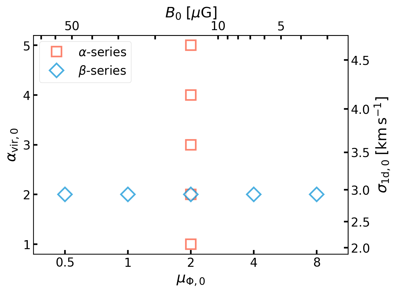
Figure 1: Parameters of simulated clouds in $\alpha$- and $\beta$-series models (see also Table 1). All clouds have the same mass $M_{\rm 0}=10^{5}\,M_{\odot}$ and radius $R_{\rm 0}=20\,{\rm pc}$. The bottom $x$-axis is the mass-to-magnetic flux ratio $\mu_{\Phi,0}=2\pi\sqrt{G}\Sigma_{\rm 0}/B_{z,0}$ and the left $y$-axis is the kinetic virial parameter $\alpha_{\rm vir,0}=5R_{\rm 0}\sigma_{\rm 1d,0}^{2}/(GM_{\rm 0})$. The top $x$-axis and right $y$-axis show the corresponding magnetic field strength $B_{z,0}$ and one-dimensional turbulent velocity dispersion $\sigma_{\rm 1d,0}$, respectively. For each pair of ($\alpha_{\rm vir,0}$, $\mu_{\Phi,0}$), we run five simulations with different random seeds for the initial turbulent velocity field.

We initialize the simulation by placing a uniform density cloud with mass $M_{\rm 0}=10^{5}\,M_{\odot}$ and radius $R_{\rm 0}=20\,{\rm pc}$ at the center of the computational domain, which has a side length $L_{\rm box}=4R_{\rm 0}=80\,{\rm pc}$. The number of grid cells is set to $256^{3}$ corresponding to the uniform grid spacing of $\Delta x=0.31\,{\rm pc}$. The cloud has the initial gas surface density $\Sigma_{\rm 0}\equiv M_{\rm 0}/(\pi R_{\rm 0}^{2})=79.6\,M_{\odot}\,{\rm pc^{-2}}$, hydrogen number density $n_{\rm H,0}=3M_{\rm 0}/(4\pi R_{\rm 0}^{3}\mu_{\rm H}m_{\rm H})=86.2\,{\rm cm}^{-3}$, and freefall time

$$t_{\rm ff,0}=\left(\frac{3\pi}{32G\rho_{0}}\right)^{1/2}=4.68\,{\rm Myr}\,.$$ (12)

The gas temperature is set to $24\,{\rm K}$ and the ${\rm H_{2}}$ abundance to the equilibrium value $x_{\rm H_{2}}=0.43$, appropriate for UV-shielded gas with $\xi_{\rm cr}=2.0\times 10^{-16}\,{\rm s}^{-1}$ (see Equations (15)–(18) in Gong et al. 2018). The ambient medium is a warm neutral medium with $n_{\rm H}=10^{-2}n_{\rm H,0}$ and $T=8200\,{\rm K}$ and has a total mass of $0.16M_{\rm 0}$. We note that we have tested the effects of the initial temperature choice, and found that they are unimportant as thermal and ionization equilibrium are rapidly achieved.

We assign the gas that is initially molecular a passive scalar field value $s_{\rm cl}=1$ and the ambient atomic gas with $s_{\rm cl}=0$. We use $s_{\rm cl}$ to differentiate the “cloud material” from the ambient medium, but it should be noted that the use of a passive scalar cannot perfectly distinguish the original cloud material due to numerical diffusion. For analysis, we select gas that is neutral and initially molecular by using a filter function

$$\Theta=\begin{cases}1,&\text{if $x_{\rm H^{+}}<0.5$ and $s_{\rm cl}>10^{-2}$}\\ 0,&\text{otherwise.}\end{cases}$$ (13)

We initiate all clouds (except the non-magnetized model) with a uniform magnetic field aligned along the $z$-axis. We note that a uniform magnetic field exerts no Lorentz force and does not play a role in supporting the cloud at $t=0$ (initial clouds are not equilibria in any case), but the nonuniform magnetic fields created by the turbulence provide support against gravity from the early stages of evolution. The initial magnetic field strength is measured by the dimensionless mass-to-magnetic flux ratio

$$\mu_{\Phi,0}=\frac{2\pi\sqrt{G}\Sigma_{\rm 0}}{B_{z,0}}$$ (14)

which is defined such that global gravitational collapse would be suppressed in subcritical clouds with $\mu_{\Phi,0}\lesssim 1$, i.e., where the mass-to-flux ratio exceeds the critical value $(2\pi\sqrt{G})^{-1}$. The parameter $\mu_{\Phi,0}^{2}$ is equal to $10/9$ of the ratio between the initial gravitational energy and magnetic energy of the cloud.

All simulations are initialized with a Gaussian-random turbulent velocity field with a power spectrum $|\delta\bm{v}_{k}|^{2}\propto k^{-4}$ for $2\leq 2\pi/L_{\rm box}\leq 64$. The corresponding structure function has velocity dispersion increasing with scale as $\sigma(\ell)\propto\ell^{1/2}$, consistent with observations of GMCs (Heyer & Brunt, 2004). We use the kinetic virial parameter

$$\alpha_{\rm vir,0}=\frac{5\sigma_{\rm 1d,0}^{2}R_{\rm 0}}{GM_{\rm 0}}$$ (15)

for an isolated, uniform, spherical cloud (Bertoldi & McKee, 1992) to quantify the level of initial turbulent support, where $\sigma_{\rm 1d,0}$ is the mass-weighted one-dimensional velocity dispersion averaged over the whole cloud. The parameter $\alpha_{\rm vir,0}$ is equal to twice the initial kinetic energy divided by the initial gravitational energy of the cloud. We note that even with a given value of $\sigma_{\rm 1d,0}$ and given power spectrum, the velocity amplitudes of individual modes differ (and therefore the cloud evolution differs) depending on the random seeds selected.

For $M_{\rm 0}=10^{5}\,M_{\odot}$, $R_{\rm 0}=20\,{\rm pc}$ and isothermal sound speed $c_{\rm s,iso}=0.26\,{\rm km}\,{\rm s}^{-1}$, the initial Alfvén speed in the cloud can be written in terms of $\mu_{\Phi,0}$ as $v_{\rm A}=B_{z,0}/\sqrt{4\pi\rho_{0}}=5.3\mu_{\Phi,0}^{-1}\,{\rm km}\,{\rm s}^{-1}$. The 3D sonic and Alfvén Mach numbers of the initial turbulence are then $\mathcal{M}_{\rm 0}=\sigma_{\rm 3d,0}/c_{\rm s,iso}=13.6\alpha_{\rm vir,0}^{1/2}$, $\mathcal{M}_{\rm A,0}=\sigma_{\rm 3d,0}/v_{\rm A}=0.67\alpha_{\rm vir,0}^{1/2}\mu_{\Phi,0}$, respectively. The plasma beta parameter in the cloud is $\beta_{0}=P/P_{\rm mag}=2c_{\rm s,iso}^{2}/v_{\rm A}^{2}=4.9\times 10^{-3}\mu_{\Phi,0}^{2}$.

To investigate the effects of the initial virial parameter and the magnetic field strength, we consider $\alpha$- and $\beta$-series models, in which either the initial kinetic or magnetic energy is held constant, while the other changes. This is equivalent to holding either $\alpha_{\rm vir,0}$ (or $\sigma_{\rm 1d,0}$) fixed or holding $\mu_{\Phi,0}$ (or $B_{z,0}$ or $\beta$) fixed, as depicted in Figure 1. In the $\alpha$-series, we vary $\alpha_{\rm vir,0}$ from 1 to 5, while the initial magnetic field is set to $B_{z,0}=13.5\mu{\rm G}$, corresponding to $\beta_{0}=0.02$ and $\mu_{\Phi,0}=2$. In the $\beta$-series, we vary $\mu_{\Phi}$ from 0.5 to 8 (by factors of two), while holding $\alpha_{\rm vir,0}=2$ (corresponding to $\sigma_{\rm 1d,0}=2.93\,{\rm km}\,{\rm s}^{-1}$). We also consider the non-magnetized case with $\mu_{\Phi,0}=\infty$. All model parameters are listed in Table 1. Our chosen parameter range for $\alpha_{\rm vir,0}$ encompasses the observational estimates of average $\alpha_{\rm vir}$ for molecular clouds in the Milky Way and nearby galaxies (e.g., Miville-Deschênes et al., 2017; Sun et al., 2018, 2020b). Except for the subcritical case $\mu_{\Phi,0}=0.5$ (which we include for theoretical completeness), the range of magnetic field strength is also consistent with the range of observed values in inter-core regions of nearby molecular clouds (a few $\mu{\rm G}$–$30\mu{\rm G}$) inferred from OH Zeeman observations (Thompson et al., 2019).

For each model we run five simulations with different random seeds for the initial turbulent velocity field. This allows us to study the variations of star formation history and cloud destruction outcomes that result from different turbulence realizations.

The name of each simulation is designated as AaBbSs, where a, b, and s respectively denote $\alpha_{\rm vir,0}$, $\mu_{\Phi,0}$, and the label of the set of random seeds used for initializing turbulence (seed). We choose the run with $\alpha_{\rm vir,0}=2$, $\mu_{\Phi,0}=2$, and ${\tt seed}=4$ as the fiducial case, for which we run additional simulations at higher ($N_{\rm cell}=512^{3}$) and lower ($N_{\rm cell}=128^{3}$) resolutions to check the numerical convergence. We present the results of our convergence test in Section 3.2 and in Table 2.

3 Evolution and Parameter Dependence

3.1 Evolution of the Fiducial Model

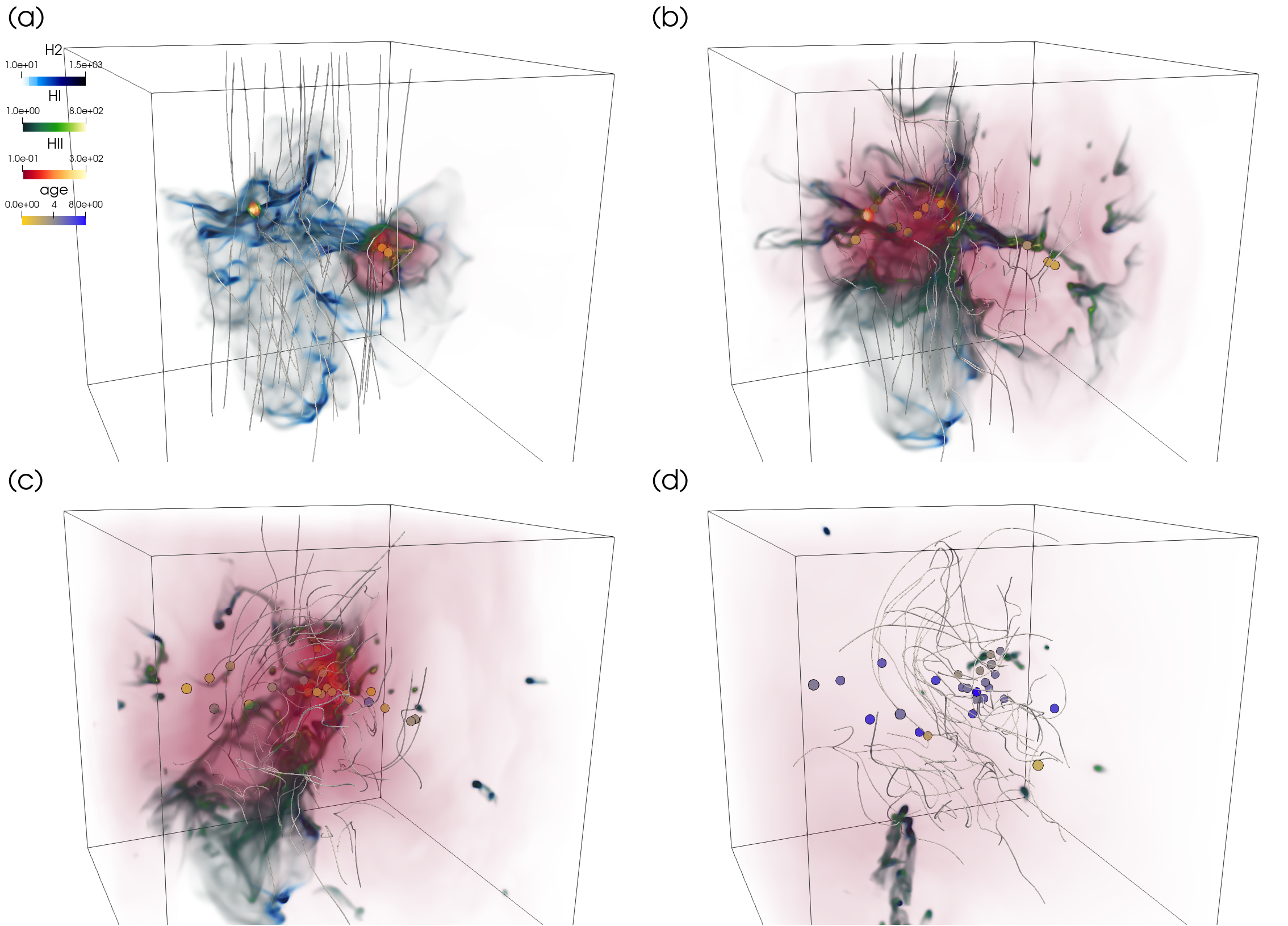
Figure 2: Volume rendering of molecular (blue-white), atomic (green-white), and ionized (red-orange) gas for the fiducial model A2B2S4 ($\alpha_{\rm vir,0}=2$, $\mu_{\Phi,0}=2$, ${\tt seed}=4$) at resolution of $256^{3}$. Panels show snapshots at (a) $t=t_{*,0}+1\,{\rm Myr}$, (b) $t_{*,0}+3\,{\rm Myr}$, (c) $t_{*,0}+5\,{\rm Myr}$, and (d) $t_{*,0}+8\,{\rm Myr}$, where $t_{*,0}=3.3\,{\rm Myr}$ is the time of first star formation. Magnetic fields are shown as lines (colored by magnitude) and star particles are shown as spheres (colored by $t_{\rm age}$). [An animation of this figure for the high-resolution model (A2B2S4_N512) is available online.]

We first sketch out the evolution of the fiducial model A2B2S4 with $(\alpha_{\rm vir,0},\mu_{\Phi,0})=(2,2)$. Figure 2 shows the volume rendering of molecular (blue-white), atomic (green-white), and ionized (red-orange) gas of the fiducial model at times $t^{\prime}\equiv t-t_{*,0}=1\,{\rm Myr}$, $3\,{\rm Myr}$, $5\,{\rm Myr}$, and $8\,{\rm Myr}$, where $t_{*,0}=3.3\,{\rm Myr}$ denotes the time at which the first star formation occurs. Magnetic field lines are visualized by lines (colored by magnitude) and star particles by spheres (colored by $t_{\rm age}$). Projections of density for snapshots at $t^{\prime}=-0.2,2,5,8\,{\rm Myr}$ of this model are also seen in the comparison figures of Appendix B.

The overall evolutionary sequence is similar to that of the hydrodynamic simulations presented in Kim et al. (2018, 2019b). The compression of gas by supersonic turbulence creates a network of dense filaments that have some preference for alignment perpendicular to the direction of the large-scale magnetic field. It also gives rise to a density probability density function (PDF) that is approximately log-normal in shape and develops a high-density tail as time progresses. At $t=3.3\,{\rm Myr}\equiv t_{*,0}$, the densest part of a filament collapses and forms the first sink particle.

Ionizing radiation from the first sink particle creates a compact and confined H II region, and the pressure of photoionized gas and (subdominant) radiation pressure force drive its dynamical expansion, suppressing further gas accretion. Once the H II region breaks out of the local star-forming clump, ionized gas quickly fills the bulk of the computational volume, and more and more UV photons escape the computational domain through optically-thin sight lines. Pre-existing dense structures are carved into pillars and cometary globules and rocket away from ionizing sources due to anisotropic ablation, as seen in other simulations of expanding H II regions in turbulent clouds (e.g., Mellema et al., 2006; Gritschneder et al., 2010; Arthur et al., 2011; Walch et al., 2012; Ali et al., 2018). Until $t^{\prime}\approx 5\,{\rm Myr}$, stellar mass continues to increase, multiple subclusters form, and H II regions merge with each other.

A substantial fraction of molecular gas at the periphery of the H II region turns into the atomic phase by dissociating radiation and then into ionized phase by ionizing radiation. Only 5% of the initial cloud mass remains molecular in the swept-up gas at $t^{\prime}=8\,{\rm Myr}$.

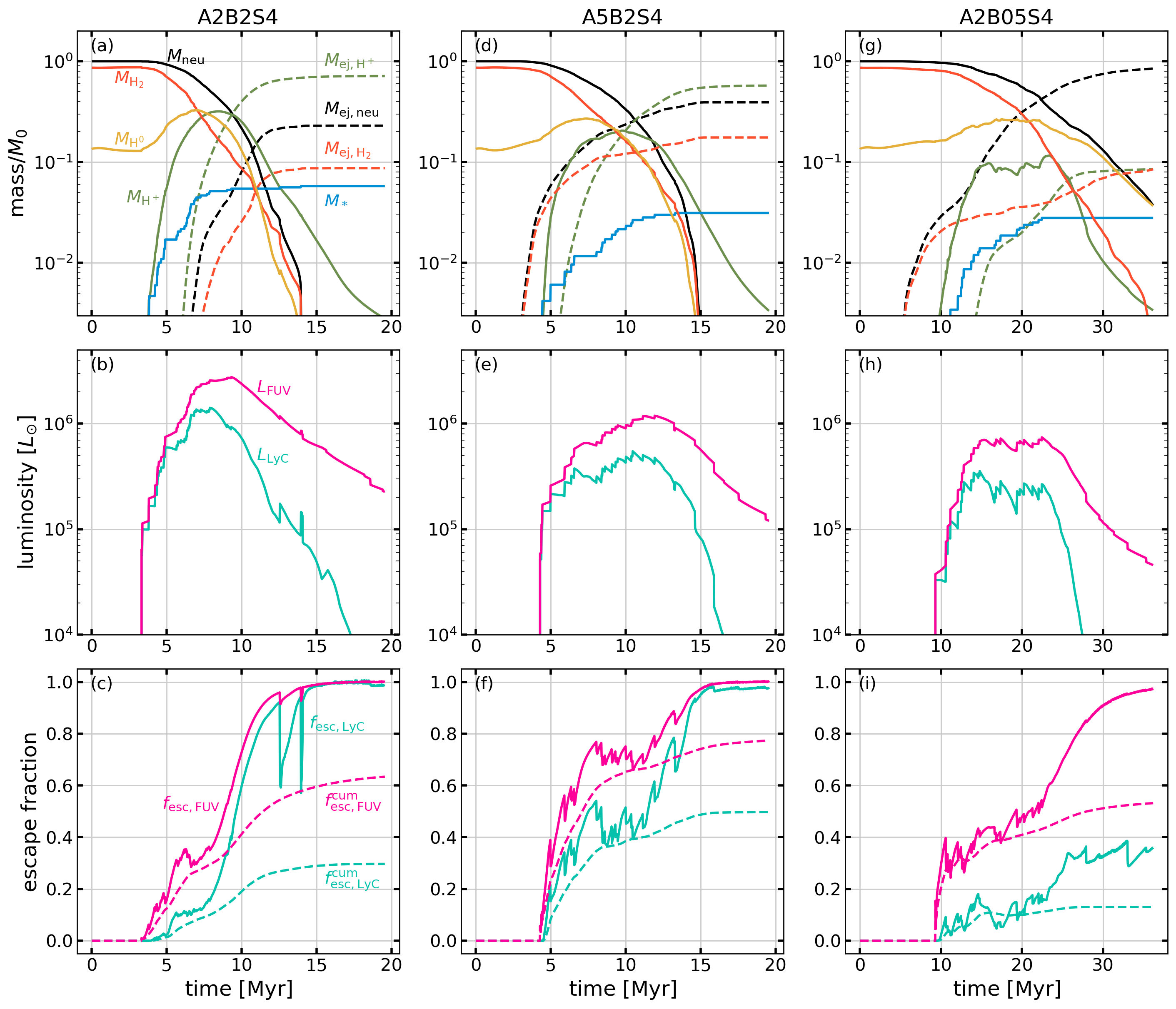
Figure 3: Time evolution of global quantities in three different models: (left) the fiducial model A2B2S4 with $(\alpha_{\rm vir,0},\mu_{\Phi,0})=(2,2)$; (middle) an initially unbound cloud A5B2S4 with $(\alpha_{\rm vir,0},\mu_{\Phi,0})=(5,2)$; (right) a magnetically subcritical cloud A2B05S4 with $(\alpha_{\rm vir,0},\mu_{\Phi,0})=(2,0.5)$. The three clouds have identical initial turbulent velocity field realizations (${\tt seed=4}$), but with different normalization for $\alpha_{\rm vir,0}=2,5$. (Top) Stellar mass ($M_{*}$), cloud gas mass in molecular ($M_{\rm H_{2}}$), atomic ($M_{\rm H^{0}}$), and ionized ($M_{\rm H^{+}}$) phases. The dashed lines show the cumulative gas mass that has left the simulation domain as neutrals ($M_{\rm ej,neu}=M_{\rm ej,H_{2}}+M_{\rm ej,H^{0}}$), ions ($M_{\rm ej,H^{+}}$), and molecules ($M_{\rm ej,H_{2}}$). (Middle) Luminosities of ionizing (LyC; cyan) and non-ionizing (FUV; magenta) photons. (Bottom) Instantaneous (solid) and cumulative (dashed) escape fractions of ionizing and non-ionizing photons.

Figure 3(a) shows the temporal evolution of the gas and stellar mass in the fiducial model. Only gas that was originally part of the cloud is shown, selected, e.g., as $M_{\rm H_{2}}=\int 2n_{\rm H_{2}}\mu_{\rm H}m_{\rm H}s_{\rm cl}dV$ where $s_{\rm cl}$ is the passive scalar for the initial cloud. The stellar mass growth (blue) is roughly linear in time and 90% of the total star formation is complete at $t^{\prime}=5.7\,{\rm Myr}$. The net SFE (or lifetime/integrated/final SFE) is $\varepsilon_{*}=M_{*,{\rm final}}/M_{\rm 0}=0.058$. Here and elsewhere, $M_{*}$ is measured based on the total mass of star particles. Photodissociation is efficient at depleting molecular gas mass: at $t^{\prime}=3.6\,{\rm Myr}$, the mass of molecular hydrogen is only $0.36M_{\rm 0}$ and the mass of atomic hydrogen increases to $0.33M_{\rm 0}$. The dashed lines show the outflow cloud gas mass that has left the computational domain as neutrals (black) and ions (green). Most (72%) of the cloud mass is photoevaporated and ejected as ions, consistent with the findings from hydrodynamic simulations of Kim et al. (2018). In addition, $22\%$ of the initial cloud is driven out as neutrals (9% molecular). We note that even without radiation feedback, a small fraction ($\sim 0.1M_{\rm 0}$) of neutrals would have been ejected; this is the portion of gas that is unbound from the initial turbulence (Raskutti et al., 2016).

In Figure 3(b) we present the evolution of the cluster luminosity in LyC and FUV (LW+PE) frequency bins for the fiducial model. The LyC (FUV) luminosity keeps increasing until $t^{\prime}=4.6\,{\rm Myr}$ ($6.0\,{\rm Myr}$) at which point $Q_{\rm LyC}=L_{\rm LyC}/h\nu_{\rm LyC}=1.9\times 10^{50}\,{\rm s}^{-1}$ ($L_{\rm FUV}=2.8\times 10^{6}\,L_{\odot}$), and decreases afterwards.

Figure 3(c) shows LyC and FUV escape fractions for the fiducial model. Instantaneous escape fractions $f_{\rm esc}(t)=L_{\rm esc}(t)/L(t)$ are plotted as solid lines while the cumulative (or luminosity-weighted, time-averaged) escape fractions $f_{\rm esc}^{\rm cum}(t)=\int_{t_{0,*}}^{t}L_{\rm esc}(t)\mathrm{d}t/\int_{t_{0,*}}^{t}L(t)\mathrm{d}t$ are shown as dashed lines. Overall, both the instantaneous and cumulative escape fractions keep increasing with time. The cumulative escape fractions measured at $t^{\prime}=3\,{\rm Myr}$ are $6.3\%$ and $24\%$ for LyC and FUV radiation, but they become as large as $30\%$ and $63\%$ at the end of the simulation ($t=19.6\,{\rm Myr}$). As we shall show, except for the magnetically subcritical clouds in which the evolutionary timescale is significantly longer than the lifetime of radiation sources, most of LyC radiation escapes in the first $5\,{\rm Myr}$ after the star formation.

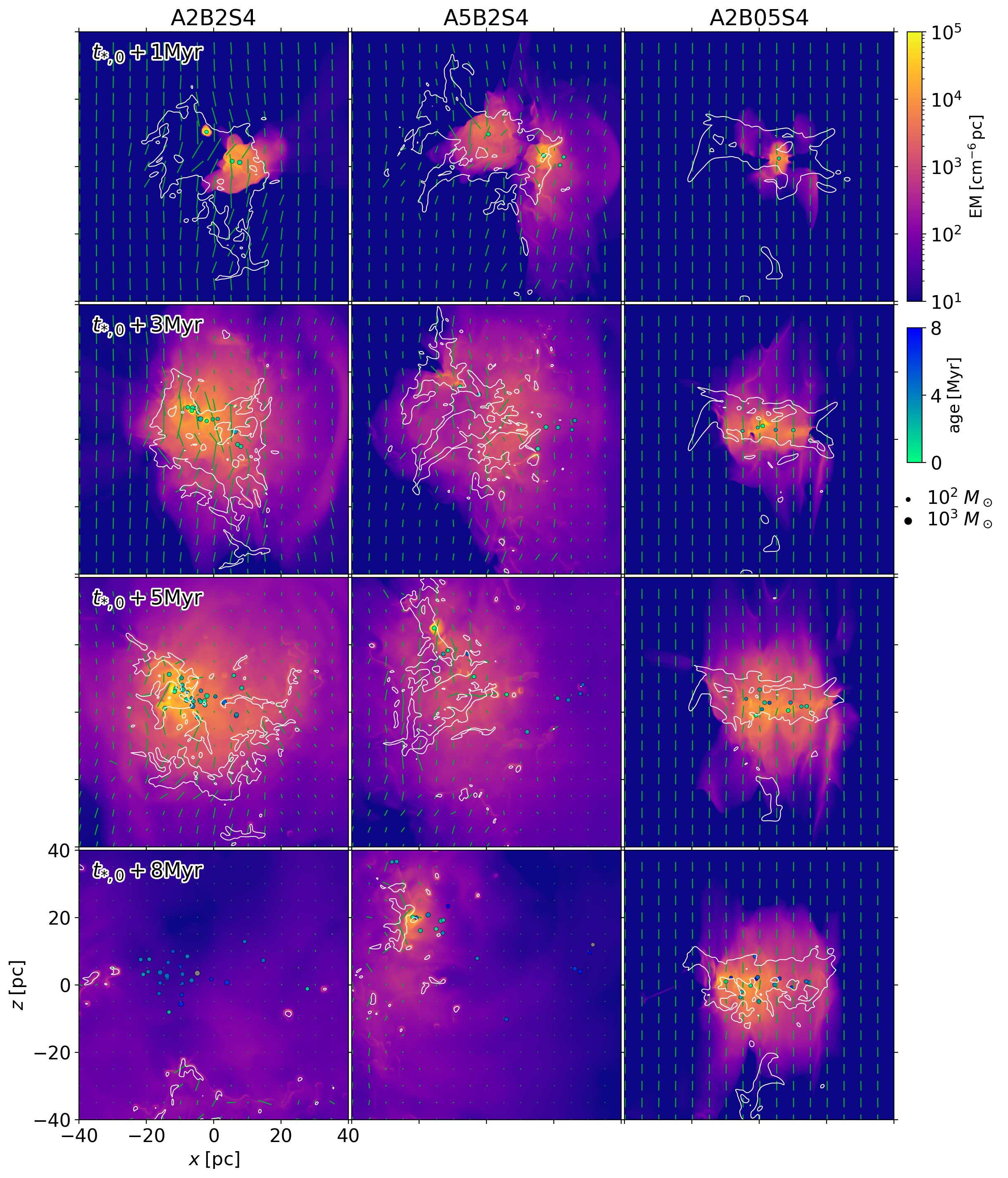
Figure 4: Emission measure along the $y$-axis of three different models (A2B2S4, A5B2S4, and A2B05S4) at times (from top to bottom) $t^{\prime}=1$, $3$, $5$, $8\,{\rm Myr}$ after the onset of star formation. The projected positions of star particles are shown as circles. Green line segments indicate the polarization vectors of dust thermal emission rotated by $90^{\circ}$, indicating the direction of magnetic field. The length of the segment is proportional to the magnitude and is normalized by the initial magnetic field $B_{z,0}$. White contours show the loci where $A_{V}=1$, corresponding to column density of neutral (atomic + molecular) hydrogen gas $1.87\times 10^{21}\,{\rm cm}^{-2}$ ($21.4\,M_{\odot}\,{\rm pc^{-2}}$).

Figure 4 depicts maps of emission measure (${\rm EM}=\int n_{\rm e}^{2}\mathrm{d}\ell$) from ionized gas projected along the $y$-axis, with snapshots from the fiducial model at $t^{\prime}=1$, $3$, $5$, $8\,{\rm Myr}$ shown in the left column of panels. Also overlaid (white contours) are the loci where $A_{V}=1$ ($N_{\rm H}=1.87\times 10^{21}\,{\rm cm}^{-2}$) in the neutral gas, outlining the overall projection of the cloud. Although at $t^{\prime}=1\,{\rm Myr}$ the H II region remains relatively confined, it has already broken out of the cloud. Over the next several Myr the region of high EM rapidly expands to cover the area of the neutral cloud and beyond. The coincidence between high EM and $A_{V}>1$ suggests that bright H$\alpha$ and CO gas would overlap for several Myr until the cloud is substantially dispersed, as seen in observations (e.g., Schinnerer et al., 2019; Chevance et al., 2020b).

Figure 4 includes overlaid line segments indicating the magnetic field orientation in the $x$-$z$ plane obtained from synthetic maps of Stokes $Q$ and $U$ parameters of polarized dust emission, assuming a spatially constant dust temperature, opacity, and intrinsic polarization fraction (e.g., Kim et al., 2019a). The length of a segment indicates the magnetic field strength normalized by the initial field strength $B_{0,z}$.

At early times a fraction of the initial kinetic energy is converted into turbulent magnetic fields. The magnetic intensity in neutral gas increases (sublinearly) with density and becomes as high as $\sim 10^{2}\,\mu{\rm G}$ in densest ($n_{\rm H}\sim 10^{4}\,{\rm cm}^{-3}$) regions. While the large-scale magnetic field orientation remains unchanged before significant gas dispersal, the small-scale magnetic field fluctuates and its orientation exhibits deviation from the large-scale orientation. Regions of higher and lower fractional polarization also reflect the facts the parallel component of the magnetic field strength is enhanced across shock fronts, but it is weakened significantly across ionization fronts after the onset of star formation (e.g., Redman et al., 1998; Draine, 2011b; Kim & Kim, 2014).

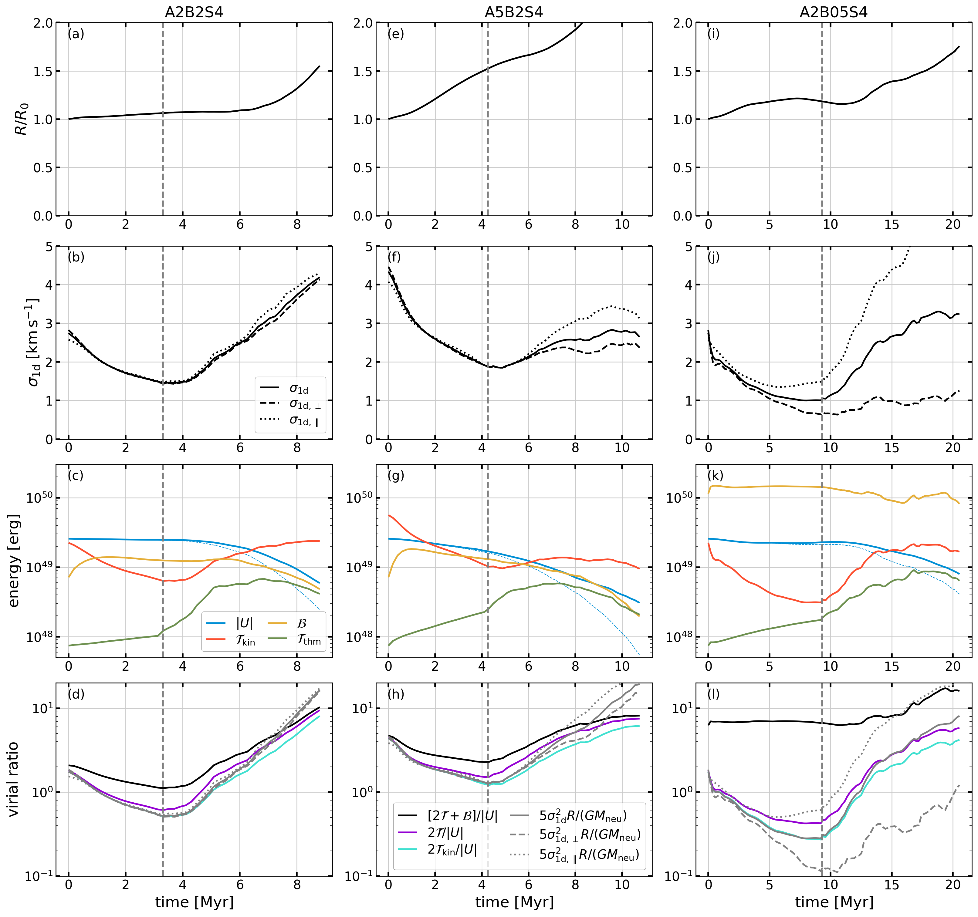
Figure 5: Time evolution of cloud size, velocity dispersion, energy, and virial ratios for three different models A2B2S4, A5B2S4, and A2B05S4 until $t_{*,90\%}$, when 90% of the final stellar mass has been formed. The grey dashed vertical lines indicate the time of first star formation. (Top row) The effective radius of neutral cloud $R=2^{1/3}R_{50\%}$, where $R_{50\%}$ is the half-mass radius. (Second row) Velocity dispersion measured perpendicular ($\sigma_{{\rm 1d},\perp}$) and parallel ($\sigma_{{\rm 1d},\parallel}$) to the background magnetic field, and averaged over all directions ($\sigma_{\rm 1d}$). (Third row) Gravitational ($|\mathcal{U}|$, blue), kinetic ($\mathcal{T}_{\rm kin}$, red), thermal ($\mathcal{T}_{\rm thm}$, green), and magnetic ($\mathcal{B}$, yellow) energies (see Equations (26)–(29)). A simple estimate of gravitational energy is also shown (blue dashed). (Fourth row) The kinetic virial parameter $\alpha_{\rm vir}=5\sigma_{\rm 1d}^{2}R/(GM_{\rm neu})$ for different viewing angles (gray lines) and various energy ratios.

The evolution of a cloud’s size and velocity dispersion reflect its dynamical evolution, both before and after the onset of radiation feedback. There are many ways to compute cloud size, but here we define the effective cloud radius as $R=2^{1/3}R_{50\%}$, where $R_{50\%}$ is the half-mass radius of the neutral gas and the factor $2^{1/3}$ applies to a homogeneous sphere ($R=R_{\rm 0}$ at $t=0$). The mass-weighted, line-of-sight velocity dispersions are measured along the Cartesian axes $\sigma_{\rm 1d,i}^{2}=\int\rho(v_{i}-\bar{v}_{i})^{2}\Theta dV/\int\rho\Theta dV$, where $\bar{v}_{i}$ is the mean velocity (see Equation (13) for definition of $\Theta$, which selects only neutral “cloud” gas). Because the gas motion is anisotropic in the presence of strong magnetic field, we consider the velocity dispersions perpendicular and parallel to the $z$-axis and their average separately:

$$\sigma_{\rm 1d,\parallel} =\sigma_{{\rm 1d},z}\,,$$ (16)

$$\sigma_{\rm 1d,\perp} =\frac{1}{\sqrt{2}}\left(\sigma_{{\rm 1d},x}^{2}+\sigma_{{\rm 1d},y}^{2}\right)^{1/2}\,,$$ (17)

$$\sigma_{\rm 1d} =\frac{1}{\sqrt{3}}\left(\sigma_{{\rm 1d},x}^{2}+\sigma_{{\rm 1d},y}^{2}+\sigma_{{\rm 1d},z}^{2}\right)^{1/2}\,.$$ (18)

The time evolution of $R$ and of $\sigma_{\rm 1d}$, $\sigma_{\rm 1d,\parallel}$, and $\sigma_{\rm 1d,\perp}$ for the fiducial model are shown in Figure 5(a) and (b). We show the time evolution until $t_{*,90\%}$, the time at which 90% of the final stellar mass has been assembled. The time of the first star formation is indicated by grey dashed vertical lines. Although gas in the cloud is compressed internally by turbulence and gravity, the overall cloud size changes very little until $t^{\prime}\sim 5\,{\rm Myr}$, when feedback begins to dominate the evolution. The decrease of the velocity dispersion before $t=t_{*,0}$ reflects the rapid decay of turbulence within a flow crossing time (e.g., Ostriker et al., 2001), but the level of the velocity dispersion begins to increase after $t^{\prime}\sim 0.5\,{\rm Myr}$ due to expanding motions induced by the radiation feedback. The velocity dispersion becomes weakly anisotropic after $t>6\,{\rm Myr}$.

Evolution of individual energies and their ratios are shown for the fiducial model in Figure 5(c) and (d); these will be discussed in detail in Section 4. Here, we simply note that as expected, the cloud’s gravitational energy ($|\mathcal{U}|$) is near constant at first and then declines (mirroring evolution of the cloud radius $R$), while kinetic energy ($\mathcal{T}_{\rm kin}$) initially drops and then increases (tracking the velocity dispersion). Magnetic energy ($\mathcal{B}$) at first increases slightly as magnetic turbulence is driven, and then declines as the cloud is dispersed.

PDFs of Density, Radiation, and Pressure

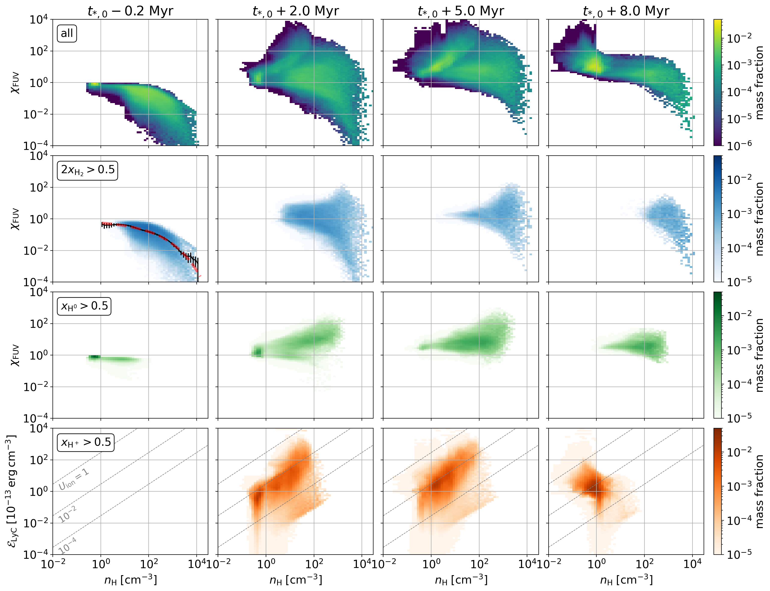
Figure 6: Mass-weighted PDFs of radiation intensity and gas density for the fiducial model (A2B2S4). at times, from left to right, $t_{*,0}-0.2\,{\rm Myr}$, $t_{*,0}+2\,{\rm Myr}$, $t_{*,0}+5\,{\rm Myr}$, $t_{*,0}+8\,{\rm Myr}$, where $t_{*,0}$ is the time of first star formation. From top to bottom, rows show the PDF of all gas, mostly-molecular gas ($2x_{\rm H_{2}}>0.5$), mostly-atomic gas ($x_{\rm H^{0}}>0.5$), and mostly-ionized gas ($x_{\rm H^{+}}>0.5$). The top three panels show the intensity in the FUV band, while the bottom row shows the intensity in the LyC band. In the left panel of the second row, the black line with error bars shows the mass-weighted average FUV intensity in molecular gas before $t_{*,0}$. This density-dependent attenuation of the ISRF is well fit by Equation (19), shown as the red dashed line. The gray dashed diagonal lines in the bottom row are the loci of constant ionization parameters (top to bottom) $U=\mathcal{E}_{\rm LyC}/(n_{\rm H}h\nu_{\rm LyC})=1$, $10^{-2}$, $10^{-4}$.

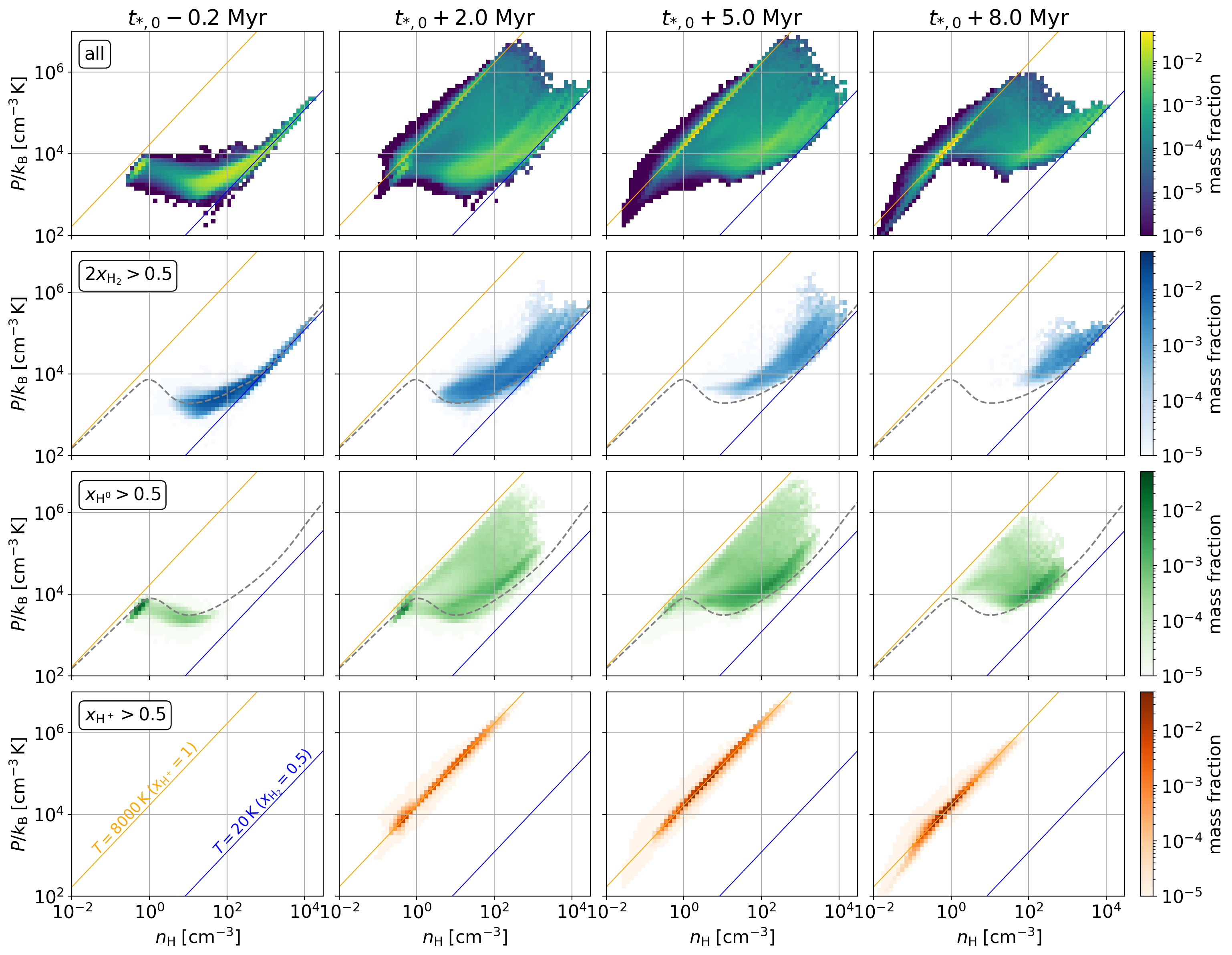
Figure 7: Mass-weighted PDF of thermal pressure and density of the fiducial model (A2B2S4). Temporal snapshots and gas phases are as in Figure 6. The blue and orange diagonal lines show constant temperature $20\,{\rm K}$ and $8000\,{\rm K}$ for fully molecular ($x_{\rm H_{2}}=0.5$) and ionized ($x_{\rm H^{+}}=1$) gas. In the second and third rows, the grey dashed lines plot the equilibrium pressure expected for gas exposed to the background UV radiation with density-dependent shielding (see text for details).

The gas in our simulations is found in a range of physical conditions. Figure 6 shows the mass-weighted PDF in the density ($n_{\rm H}$) and radiation intensity ($\chi_{\rm FUV}$ or $\mathcal{E}_{\rm LyC}$) plane at times $t^{\prime}=-0.2$, $2$, $5$, $8\,{\rm Myr}$. The top row shows the PDF of the entire gas, while the other rows select gas in molecular ($2x_{\rm H_{2}}>0.5$; blue), neutral atomic ($x_{\rm H^{0}}>0.5$; green), and ionized ($x_{\rm H^{+}}>0.5$; orange) phases. In the top three rows of Figure 6, we show the distribution in the $n_{\rm H}$–$\chi_{\rm FUV}$ plane; in the bottom row we plot the distribution in the $n_{\rm H}$–$\mathcal{E}_{\rm LyC}$ plane. Similarly, Figure 7 shows mass-weighted PDFs in the density and pressure ($P/{\,k_{\rm B}}$) plane.

Before the onset of massive star formation ($t_{*,0}-0.2\,{\rm Myr}$ panels), gas is subject to the background FUV radiation only. The ambient gas is optically thin, and is therefore exposed to the ISRF with $0.8\lesssim\chi_{\rm FUV}\leq 1$; it has low density and is in the warm ($T\sim 8000\,{\rm K}$) atomic phase. The width of the density PDF of the ambient warm gas is narrow as turbulence is subsonic.

The cold, dense gas in the cloud is subject to a range of FUV intensity and becomes increasingly shielded at higher density. Most of the cloud is molecular, as shown in Figure 3(a). For the fiducial cloud, we compute the mass-weighted mean FUV intensity in each density bin for snapshots before the first star formation. In the left panel of the second row in Figure 6, the black line shows the time-averaged mean FUV intensity $\chi_{\rm FUV,avg}$ for snapshots prior to the onset of star formation, with the error bars indicating the standard deviation. We find that $\chi_{\rm FUV,avg}$ has weak temporal variation and is well described by a local shielding approximation. The red dashed line shows that the average FUV radiation field in molecular gas with $n_{\rm H}>1\,{\rm cm}^{-3}$ is well fit by the function $\chi_{\rm FUV,avg}=0.9e^{-\tau_{\rm FUV,eff}}$, where the effective optical depth is fitted as a power-law function of gas density:

$$\tau_{\rm FUV,eff}=1.8\left(\frac{n_{\rm H}}{10^{2}\,{\rm cm}^{-3}}\right)^{0.30}\,;$$ (19)

$1.8$ and $0.30$ are the best-fit parameters. That is, the effective optical depth increases sublinearly with density, such that if we define $\tau_{\rm FUV,eff}\equiv\sigma_{\rm d}n_{\rm H}L_{\rm shld}$, this corresponds to the shielding length of $L_{\rm shld}\sim 6\,{\rm pc}$ when $n_{\rm H}=10^{2}\,{\rm cm}^{-3}$.

Based on this result, we calculate the equilibrium chemical abundances and temperature of molecular gas as a function of $n_{\rm H}$ assuming constant $\xi_{\rm cr}=2\times 10^{-16}\,{\rm s}^{-1}$, and density-dependent FUV intensity $\chi_{\rm FUV,avg}$. We also calculate the equilibrium curve for unshielded atomic gas assuming $\xi_{\rm cr}=2\times 10^{-16}\,{\rm s}^{-1}$, $\chi_{0}=1$, and $\tau_{\rm FUV,eff}=0$. The gray dashed lines in center two rows of Figure 7 show the resulting equilibrium curves; before the onset of star formation most gas remains close to these equilibrium curves. The low-density molecular gas with $10\,{\rm cm}^{-3}<n_{\rm H}<10^{3}\,{\rm cm}^{-3}$ exhibits a range of temperature $20\,{\rm K}<T<100\,{\rm K}$, while the high-density molecular gas for which the heating is dominated by cosmic ray ionization has a constant temperature of $\sim 20\,{\rm K}$ (blue diagonal lines in Figure 7). The thermal pressure of the atomic and diffuse molecular gas ranges from $P/k_{\rm B}\sim 10^{3}$–$10^{4}\,{\rm cm}^{-3}\,{\rm K}$, while it can be as high as $\sim 2\times 10^{5}\,{\rm cm}^{-3}\,{\rm K}$ at the density of sink particle formation ($\sim 2\times 10^{4}\,{\rm cm}^{-3}$).

After the onset of massive star formation ($t^{\prime}>0$), both neutrals and ions are subject to intense UV radiation from newborn stars, and the normalized FUV radiation intensity can be as high as $\chi_{\rm FUV}\sim 10^{2}$ in the photon dominated region (PDR). The temperature of lightly-shielded dense molecular/atomic gas in the PDR is significantly elevated because of enhanced heating, but most of the gas is still shielded and remains cold, at $T\sim 20$–$100\,{\rm K}$. The photoionized gas has temperature $\sim 8000\,{\rm K}$ (orange diagonal lines in Figure 7). The ionized gas has a range of ionization parameter $U_{\rm ion}=\mathcal{E}_{\rm LyC}/(h\nu_{\rm LyC}n_{\rm H})$, but most falls in the range $10^{-2.5}$–$10^{-1.5}$ (see gray dashed diagonal lines in the bottom row of Figure 6).

3.2 Evolution of Other Models

While the overall evolution of other models is similar to that of the fiducial model, there are a few notable differences. Here we give an overview of other simulations and take two extreme cases, one with the strongest initial turbulence/highest $\alpha_{\rm vir,0}$ (A5B2S4) and the other with the strongest initial magnetic field/lowest $\mu_{\Phi,0}$ (A2B05S04), to compare and contrast with the fiducial model. Results from these two extreme models are shown in the middle and right columns of Figures 3, 4, 5. In addition, in Appendix B we compare a series of snapshots of projected column density from members of the $\alpha$-series in Figure 18 (all with ${\tt seed}=4$), members of the $\beta$-series models in Figure 19 (all with ${\tt seed}=4$), and the fiducial model (A2B2) with initial different turbulence realizations (i.e., varying seed but the same initial kinetic and magnetic energy) in Figure 20.

Our key simulation results are summarized in Table 2. Quantitative comparisons of star formation history, SFE, ionized and neutral gas ejection, timescale for star formation/cloud destruction, and escape fraction of radiation from all models will be presented in Sections 3.3–3.7. Comparisons of virial parameter evolution and efficiency per freefall time, also connecting with observations, will be discussed in Sections 4 and 5, respectively.

The bottom three rows of Table 2 show results from the fiducial model (${\tt A2B2S4}$) run at higher ($N_{\rm cell}=512^{3}$) and lower ($N_{\rm cell}=128^{3}$) resolutions. These tests demonstrate numerical convergence of our results, within the range of variation that is expected from turbulence-induced stochasticity in the evolution.

3.2.1 Dependence on $\alpha_{\rm vir,0}$

Even at quite early times, the extent of the molecular cloud systematically changes with $\alpha_{\rm vir,0}$. The left panels of Figure 18 in Appendix B show that the cloud with the lowest initial virial parameter (A1B2S4, with $\alpha_{\rm vir,0}=1$) initially contracts in size as turbulent pressure support is insufficient to counteract gravity. In contrast, clouds that are initially unbound have a larger fraction of their material at velocity greater than the escape speed of the cloud, and expand rapidly over the first few Myr of evolution. This has the effect of both directly enhancing the mass loss of neutrals and reducing the gas surface density during the star-forming epoch, both of which contribute to a systematically lower net SFE at higher $\alpha_{\rm vir,0}$.

In part because the turbulent shear is more effective in dispersing overdense structures before they collapse in the higher-$\alpha_{\rm vir,0}$ models, the time of the first star formation $t_{*,0}$ is nearly 1 Myr (on average) earlier in the lowest-$\alpha_{\rm vir,0}$ models compared to the highest–$\alpha_{\rm vir,0}$ models. Comparing Figure 3(a) and (d), even though the lifetime SFE is lower in the $\alpha_{\rm vir,0}=5$ model compared to the $\alpha_{\rm vir,0}=2$ model, “active” star formation continues over a longer period in the $\alpha_{\rm vir,0}=5$ model (up to $t\sim 11\,{\rm Myr}$, compared to $t\sim 9\,{\rm Myr}$) because the cloud is not as rapidly dispersed when the star formation and resulting feedback is less vigorous. Still, there is late-time residual star formation in the $\alpha_{\rm vir,0}=2$ model, and the overall beginning-to-end duration of star formation does not show strong dependence on $\alpha_{\rm vir,0}$ across models (see Section 3.6).

We also note, as can be seen from the comparisons in Figure 4 and Figure 18, that distribution of radiation sources is less compact in high-$\alpha_{\rm vir,0}$ compared to low-$\alpha_{\rm vir,0}$ models.

3.2.2 Dependence on $\mu_{\Phi,0}$

Our simulation suite includes both strongly magnetized clouds (with the $\mu_{\Phi,0}=0.5$ case even subcritical) and weakly magnetized clouds. The latter (models $\mu_{\Phi,0}=4$ and $8$) have initial $B_{z,0}<10\mu{\rm G}$, and the magnetic field remain energetically subdominant – with super-Alfvénic turbulence – throughout their lifetimes. Their overall evolution and morphological characteristics are largely similar to the fiducial model. We also include an unmagnetized model. Compared to the non-magnetized run, the first star formation event in moderate-magnetization models is a bit delayed ($\sim 0.5$–$1\,{\rm Myr}$), and SFR and net SFE are slightly lower.

The magnetically subcritical and critical clouds ($\mu_{\Phi,0}=0.5$ and $1$) have initial magnetic fields $54\mu{\rm G}$ and $27\mu{\rm G}$, with initially sub-Alfvénic turbulence. Figure 19 shows that overdense filamentary structures preferentially aligned perpendicular to $\bm{B}_{0}$ along the $z$-axis (to an extreme degree in the subcritical case). The strong magnetic field constrains motions to proceed primarily along the $z$-axis, and as a result the cloud expansion driven by feedback at late times is highly anisotropic in these models.

Compared to the fiducial model, in the subcritical and critical cases the strong magnetic field both delays the onset of star formation and reduces the SFR. As a result, it takes longer to build up enough stellar mass that the feedback is sufficient to disperse the residual gas. In addition, the reduced gas compressibility and strong magnetic tension force make cloud structure less porous and H II regions remain confined for a longer period of time. This makes the escape of ionized gas and ionizing radiation more difficult. For these reasons, only a small fraction of gas is photoevaporated by LyC in the critical and subcritical cases. Compared to the fiducial model, in which most of the mass loss is in ionized gas, nearly 10 times as much gas is dispersed in the neutral phase as the ionized phase.

In fact, the evolution of magnetically subcritical clouds are unusual in several aspects. In A2B05S4, the first star formation occurs at $9.3\,{\rm Myr}$ and the net SFE is only $2.8\%$. The stellar mass builds up on a timescale that is long compared to the lifetime of ionizing luminosity (see Figure 3g, h). Due to the low luminosity, gas dispersal takes place steadily over a very long period ($\sim 20\,{\rm Myr}$), the mass loss by photoevaporation is much less effective than in the fiducial model, and the LyC escape fraction does not reach a high value even at late times (Figure 3(g)). The evolution of $\sigma_{\rm 1d}$ (Figure 5(j)) shows that the motion of neutral gas becomes highly anisotropic after the onset of feedback, with motions almost entirely parallel to the background magnetic field. The map of EM in Figure 4 shows that ionized gas outflows follow the magnetic field lines, and that the cloud dispersal is incomplete even at $t^{\prime}=8\,{\rm Myr}$ (see also the right panels in Figure 3). The final frame of Figure 19 for the $\mu_{\Phi,0}=0.5$ model shows an essentially columnar outflow. Lack of evidence for these unusual morphological features in observations suggests that at GMC scales, real clouds are generally magnetically critical or supercritical. Some lower mass dark clouds (without massive star formation) may, however, be magnetically subcritical (see Section 6). In addition, smaller-scale bipolar H II regions have been identified by Deharveng et al. (2015); Eswaraiah et al. (2017), suggesting localized strong magnetic fields, perhaps enhanced by the collapse that created the exciting clusters.

3.2.3 Dependence on Turbulence Realization

For each model in the $\alpha$- and $\beta$-series, we run five simulations with different random realizations for the initial turbulence. The initial large-scale velocity field and its orientation relative to the field line affect the specifics of when and where dense structures form, which in turn affect the subsequent cluster formation and cloud evolution. As a result, the simulation outcome exhibits a moderate degree of variation with random seeds. Figure 20 shows snapshots of the fiducial model with different turbulence realizations. We find that runs with ${\tt seed}=1$ and $5$ form centrally-concentrated dense filaments, which are favorable to an early, rapid burst of star formation (see second column in Figure 20). In contrast, overdense structures in runs with ${\tt seed}=2$ and $3$ are spatially separated from each other, and these models have slower SFR and lower SFE. While some of the same trends with seed persist in other models with different $\alpha_{\rm vir,0}$ or $\mu_{\Phi,0}$, not all quantitative outcomes systematically vary with the random seed (see Sections 3.3–3.7).

For a given total kinetic energy, lower SFR and SFE in some turbulent realizations may simply be due to more of the large-scale modes (which contain most of the energy) favoring expansion or shear rather than compression.

3.3 Star Formation History and Rate

Table 2: Simulation results

Model	$t_{*,0}$	$\tilde{\alpha}_{\rm vir,tot}(t_{*,0})$	$\varepsilon_{*}$	$\varepsilon_{*,{\rm 3\,Myr}}$	$\varepsilon_{\rm ion}$	$\varepsilon_{\rm ej,neu}$	$t_{\rm SF}$	$t_{\rm dest,H_{2}}$	$t_{\rm dep,0}$	$\varepsilon_{\rm ff,0}$	$\langle f_{\rm esc,LyC}\rangle$	$\langle f_{\rm esc,FUV}\rangle$
	[Myr]		[%]	[%]	[%]	[%]	[Myr]	[Myr]	[Myr]	[%]	[%]	[%]
(1)	(2)	(3)	(4)	(5)	(6)	(7)	(8)	(9)	(10)	(11)	(12)	(13)
$\alpha$-series
A1B2	$3.5^{+0.6}_{-0.4}$	$0.86^{+0.07}_{-0.07}$	$9.5^{+2.9}_{-1.8}$	$5.6^{+1.3}_{-0.6}$	$73.2^{+1.1}_{-2.9}$	$17.4^{+3.5}_{-2.2}$	$5.0^{+0.3}_{-0.2}$	$7.4^{+0.7}_{-0.8}$	$58^{+6}_{-13}$	$8.0^{+2.4}_{-0.8}$	$21.0^{+4.6}_{-7.6}$	$52.7^{+4.3}_{-10.5}$
A2B2	$3.8^{+0.5}_{-0.5}$	$1.10^{+0.02}_{-0.10}$	$5.8^{+2.1}_{-1.4}$	$2.6^{+2.4}_{-1.1}$	$71.7^{+2.2}_{-0.7}$	$21.9^{+2.8}_{-2.6}$	$5.4^{+0.3}_{-1.1}$	$7.6^{+0.2}_{-0.8}$	$99^{+52}_{-39}$	$4.7^{+3.0}_{-1.6}$	$26.7^{+3.0}_{-0.5}$	$62.4^{+1.0}_{-5.1}$
A3B2	$3.7^{+1.3}_{-0.4}$	$1.43^{+0.02}_{-0.14}$	$4.1^{+2.2}_{-1.5}$	$1.9^{+2.0}_{-0.7}$	$68.3^{+3.4}_{-7.7}$	$28.7^{+8.2}_{-6.3}$	$5.5^{+1.1}_{-1.1}$	$7.5^{+0.5}_{-0.1}$	$149^{+78}_{-52}$	$3.2^{+1.7}_{-1.1}$	$27.6^{+12.9}_{-3.4}$	$65.9^{+3.0}_{-4.8}$
A4B2	$4.1^{+1.1}_{-0.9}$	$1.77^{+0.13}_{-0.16}$	$3.6^{+0.6}_{-1.9}$	$1.7^{+0.4}_{-0.7}$	$63.1^{+4.5}_{-15.9}$	$33.2^{+17.9}_{-4.8}$	$6.3^{+0.2}_{-1.2}$	$7.4^{+0.5}_{-0.6}$	$163^{+190}_{-11}$	$2.9^{+0.2}_{-1.5}$	$34.2^{+8.3}_{-9.4}$	$67.8^{+4.6}_{-0.1}$
A5B2	$4.3^{+1.3}_{-0.9}$	$2.12^{+0.17}_{-0.09}$	$2.1^{+1.1}_{-1.2}$	$1.2^{+0.2}_{-0.6}$	$48.3^{+9.4}_{-19.5}$	$49.6^{+20.4}_{-10.4}$	$5.3^{+1.5}_{-0.9}$	$8.3^{+0.5}_{-1.3}$	$255^{+313}_{-31}$	$1.8^{+0.3}_{-1.0}$	$31.2^{+18.5}_{-17.1}$	$68.8^{+8.6}_{-3.2}$
$\beta$-series
A2B05	$8.6^{+4.7}_{-2.1}$	$6.66^{+1.76}_{-0.74}$	$2.4^{+1.2}_{-0.5}$	$0.5^{+0.3}_{-0.1}$	$12.4^{+5.0}_{-7.5}$	$83.5^{+2.2}_{-4.7}$	$12.0^{+3.5}_{-3.1}$	$17.3^{+4.8}_{-1.4}$	$464^{+401}_{-163}$	$1.0^{+0.5}_{-0.5}$	$13.1^{+0.3}_{-4.8}$	$56.5^{+1.7}_{-6.8}$
A2B1	$4.4^{+2.4}_{-0.9}$	$2.18^{+0.34}_{-0.20}$	$4.3^{+1.8}_{-1.8}$	$1.5^{+0.5}_{-0.9}$	$35.3^{+17.7}_{-8.7}$	$54.2^{+5.5}_{-13.9}$	$6.9^{+1.3}_{-1.1}$	$9.4^{+0.7}_{-1.0}$	$182^{+103}_{-59}$	$2.6^{+1.2}_{-0.9}$	$21.1^{+2.8}_{-9.5}$	$58.3^{+2.5}_{-1.7}$
A2B2	$3.8^{+0.5}_{-0.5}$	$1.10^{+0.02}_{-0.10}$	$5.8^{+2.1}_{-1.4}$	$2.6^{+2.4}_{-1.1}$	$71.7^{+2.2}_{-0.7}$	$21.9^{+2.8}_{-2.6}$	$5.4^{+0.3}_{-1.1}$	$7.6^{+0.2}_{-0.8}$	$99^{+52}_{-39}$	$4.7^{+3.0}_{-1.6}$	$26.7^{+3.0}_{-0.5}$	$62.4^{+1.0}_{-5.1}$
A2B4	$3.1^{+0.1}_{-0.4}$	$0.93^{+0.05}_{-0.16}$	$6.9^{+1.6}_{-1.9}$	$3.4^{+1.0}_{-0.6}$	$79.0^{+4.8}_{-1.9}$	$13.9^{+2.8}_{-6.1}$	$4.9^{+2.2}_{-0.7}$	$6.9^{+2.1}_{-0.4}$	$84^{+20}_{-22}$	$5.5^{+2.0}_{-1.1}$	$25.8^{+10.9}_{-2.5}$	$61.3^{+3.5}_{-5.3}$
A2B8	$2.6^{+0.2}_{-0.1}$	$0.92^{+0.12}_{-0.15}$	$7.4^{+2.3}_{-0.1}$	$3.7^{+0.7}_{-0.1}$	$82.3^{+2.4}_{-1.4}$	$9.2^{+1.5}_{-1.2}$	$5.4^{+1.0}_{-1.1}$	$7.4^{+0.7}_{-0.4}$	$75^{+16}_{-13}$	$6.3^{+1.3}_{-1.1}$	$33.0^{+4.5}_{-9.3}$	$64.2^{+2.6}_{-7.8}$
A2Binf	$2.1^{+0.2}_{-0.5}$	$1.00^{+0.27}_{-0.07}$	$8.2^{+1.3}_{-1.1}$	$5.1^{+1.7}_{-1.1}$	$82.6^{+2.7}_{-0.6}$	$8.1^{+1.7}_{-1.6}$	$4.1^{+0.8}_{-0.2}$	$6.4^{+0.4}_{-0.5}$	$61^{+8}_{-14}$	$7.7^{+2.2}_{-0.9}$	$30.7^{+5.5}_{-2.5}$	$63.3^{+3.4}_{-1.9}$
A2B2S4_N128	$3.1$	$1.23$	$6.1$	$3.1$	$68.1$	$25.9$	$6.5$	$7.9$	$109$	$4.3$	$31.4$	$63.1$
A2B2S4_N256	$3.3$	$1.12$	$5.8$	$2.5$	$71.7$	$23.0$	$5.7$	$7.6$	$99$	$4.7$	$29.7$	$63.4$
A2B2S4_N512	$3.2$	$1.11$	$5.0$	$1.9$	$71.6$	$23.9$	$5.1$	$7.9$	$126$	$3.7$	$28.7$	$62.1$

Note. — For each model in the $\alpha$- and $\beta$-series there are 5 realizations of turbulence. The reported values are medians, and the superscript (subscript) refers to the difference to the maximum (minimum) value. Results from tests at lower and higher (only $\tt seed$=4) resolution are given in bottom two rows. Columns are as follows (1): model name indicating the initial virial parameter (A) and the magnetic flux-to-mass ratio (B). (2): time of first star formation. (3): virial parameter $\tilde{\alpha}_{\rm vir,tot}=(2\mathcal{T}+\mathcal{B})/|\mathcal{U}|$ at $t_{*,0}$. (4): final SFE $\varepsilon_{*}=M_{*}/M_{0}$. (5): SFE at $t^{\prime}=3\,{\rm Myr}$. (6): photoevaporation efficiency. (7): ejected neutral efficiency. (8): star formation duration needed to assemble 90% of the final stellar mass. (9): cloud destruction time needed to reach $M_{\rm H_{2}}=0.05M_{\rm 0}$. (10): gas depletion time $t_{\rm dep,0}=M_{\rm 0}/\langle\dot{M}_{*}\rangle$. (11): SFE per freefall time $\varepsilon_{\rm ff,0}=t_{\rm ff,0}/t_{\rm dep,0}$ (12)–(13): cumulative (or luminosity-weighted mean) escape fractions of ionizing (LyC) and non-ionizing (FUV) radiation.

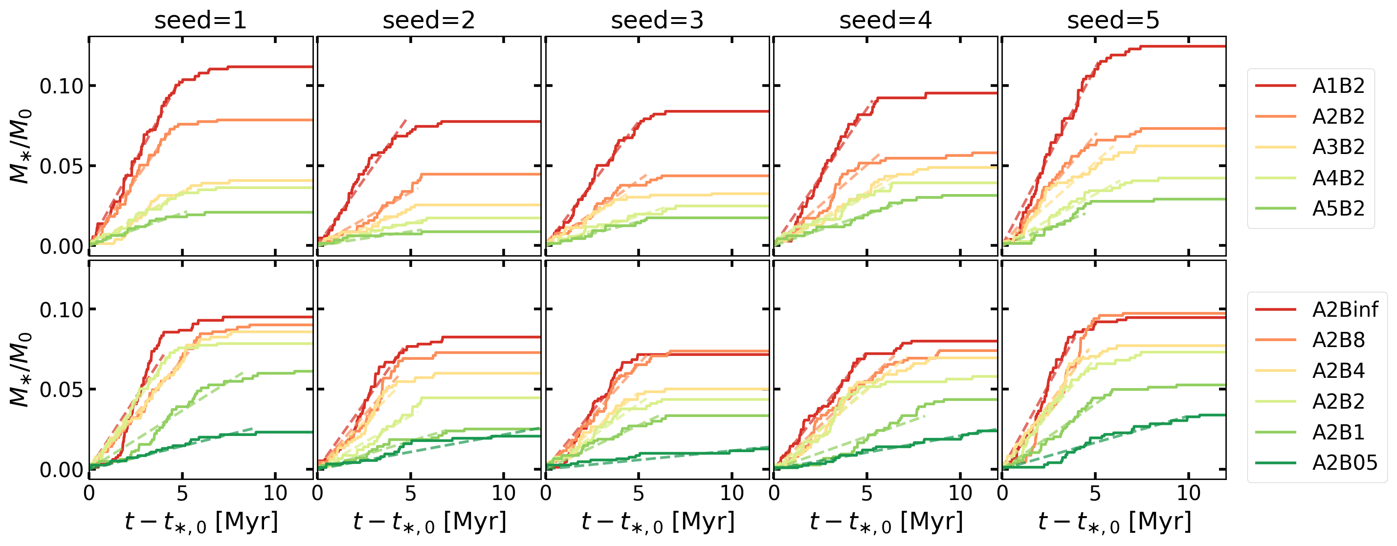
Figure 8: Star formation history of all models with different seeds. The upper/lower panels show $\alpha$/$\beta$-series models. Time is measured from the moment of first star formation $t_{*,0}$. The dashed lines represent a linear least square fit for the time range $t_{*,0}<t<t_{*,90\%}$, where $t_{*,90\%}$ is the time at which 90% of the final stellar mass has been assembled. We use the slope of the line as the time averaged SFR $\langle\dot{M}_{*}\rangle$.

We compare star formation history of all models in Figure 8, which shows the stellar mass $M_{*}$ as a function of $t^{\prime}=t-t_{*,0}$ in the $\alpha$-series (top) and $\beta$-series (bottom) models. Different initial turbulence realizations are labeled by seed$=1$–$5$ (left to right).

The stellar mass growth occurs over several Myrs in a “stair-stepping” fashion due to our finite mass resolution (typical initial sink mass is about $10^{-3}M_{\rm 0}$). It is roughly linear during the main phase of star formation and levels off once the radiative feedback takes over. Some models exhibit a few episodic star formation events that take place in swept-up gas at the periphery of H II regions at late times.

We quantify the time-averaged SFR, $\langle\dot{M}_{*}\rangle$, during the main period of star formation by performing a least square fit to a function $M_{*}(t)=\langle\dot{M}_{*}\rangle t$ for the time interval $(t_{*,0},t_{*,90\%})$. The results are shown as dashed lines in Figure 8, suggesting that linear mass growth is a good approximation for most of our models. Except for the runs with ${\tt seed}=1$ in the $\beta$-series, the mean SFR monotonically increases with decreasing $\alpha_{\rm vir,0}$ and with increasing $\mu_{\Phi,0}$. That is, higher kinetic and magnetic energy reduce the SFR, for a given cloud mass and size.

3.4 Star Formation Efficiency

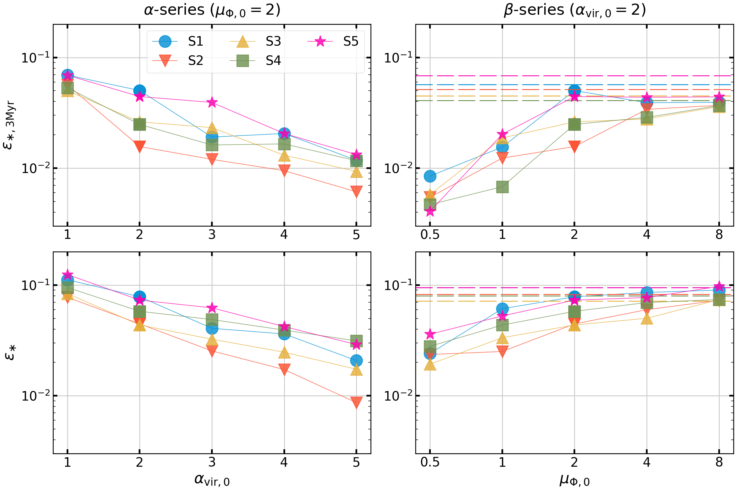
Figure 9: SFE at time $3\,{\rm Myr}$ after the first star formation ($\varepsilon_{*,3\,{\rm Myr}}$; top) and final star formation efficiency ($\varepsilon_{*}$; bottom), in models with varying initial kinetic or magnetic energy or turbulence realization. The $\alpha$-series is shown to the left and $\beta$-series to the right, with simulation runs having different turbulent realizations as marked by seed with different colors/symbols. Horizontal dashed lines in the right panels indicate the values for the unmagnetized models (A2Binf). Higher initial turbulence level (larger $\alpha_{\rm vir,0}$) or magnetization (smaller $\mu_{\Phi,0}$) reduces the SFE.

Figure 8 shows that clouds in our simulations convert only a small fraction of the initial gas mass into stars over their lifetimes. In Figure 9, we show the SFE at $t^{\prime}=3\,{\rm Myr}$ ($\varepsilon_{*,3\,{\rm Myr}}$) and the lifetime SFE ($\varepsilon_{*}$) in the $\alpha$- (left) and $\beta$-series (right) models. For each model, we show runs with different turbulent seeds with different symbols and colors. For the $\beta$-series models, the results of non-magnetized runs are shown as horizontal dashed lines. The time $t^{\prime}=3\,{\rm Myr}$ is chosen to provide an estimate of the SFE at the time of the first supernova. In Columns (4) and (5) of Table 2 we list result for medians (over seed) of $\varepsilon_{*}$ and $\varepsilon_{*,3\,{\rm Myr}}$, and give differences to the minimum/maximum values with superscripts/subscripts. For example, the fiducial model (A2B2) has net SFE of $\varepsilon_{*}=5.8^{+2.1}_{-1.4}\%$ for the 5 different runs.

For fixed turbulent realization, Figure 8 shows that final stellar mass decreases with increasing $\alpha_{\rm vir,0}$ and decreasing $\mu_{\Phi,0}$. The median (over seed) net SFE in the $\alpha$-series ranges between $\varepsilon_{*}=2.1\%$ and $9.5\%$, increasing for lower kinetic energy (lower $\alpha_{\rm vir,0}$). The median net SFE in the $\beta$-series models ranges between $\varepsilon_{*}=2.4\%$ and $8.2\%$, increasing for lower magnetization (higher $\mu_{\Phi,0}$). In all models, different turbulence realizations can produce variations at a level of a few percent in the SFE. Although the absolute variations in SFE are small, this amounts to up to factor of $2$–$3$ range in $\varepsilon_{*,3\,{\rm Myr}}$ and $\varepsilon_{*}$ for different turbulence realizations. Most of our simulated clouds have formed about $\sim 50^{+20}_{-20}\%$ of the final stellar mass at $t^{\prime}=3\,{\rm Myr}$. The exceptions are the very strongly-magnetized models A2B05 and A2B1, in which $\varepsilon_{*,3\,{\rm Myr}}/\varepsilon_{*}\sim 0.25$ as they have significantly longer star formation duration (see Section 3.6).

The simulations of Kim et al. (2018) were purely hydrodynamic, including a model analogous to ${\tt seed}=1$ and $\mu_{\Phi,0}=\infty$, which resulted in $\varepsilon_{*}=13\%$, somewhat higher than $9.6\%$ of our model ${\tt A2BinfS1}$. This difference is likely to be caused by the inclusion of more realistic thermochemical processes in our new simulations; the temperature of molecular gas in the PDR is raised significantly due to the FUV heating, which makes the collapse of dense structures more difficult at late times (e.g., Inoguchi et al., 2020). Considering the stochastic nature of the system, these differences can also induce other changes; as we have shown, different realizations of turbulence lead to variations in SFE of a few percent.

3.5 Photoevaporation and Ejection Efficiencies

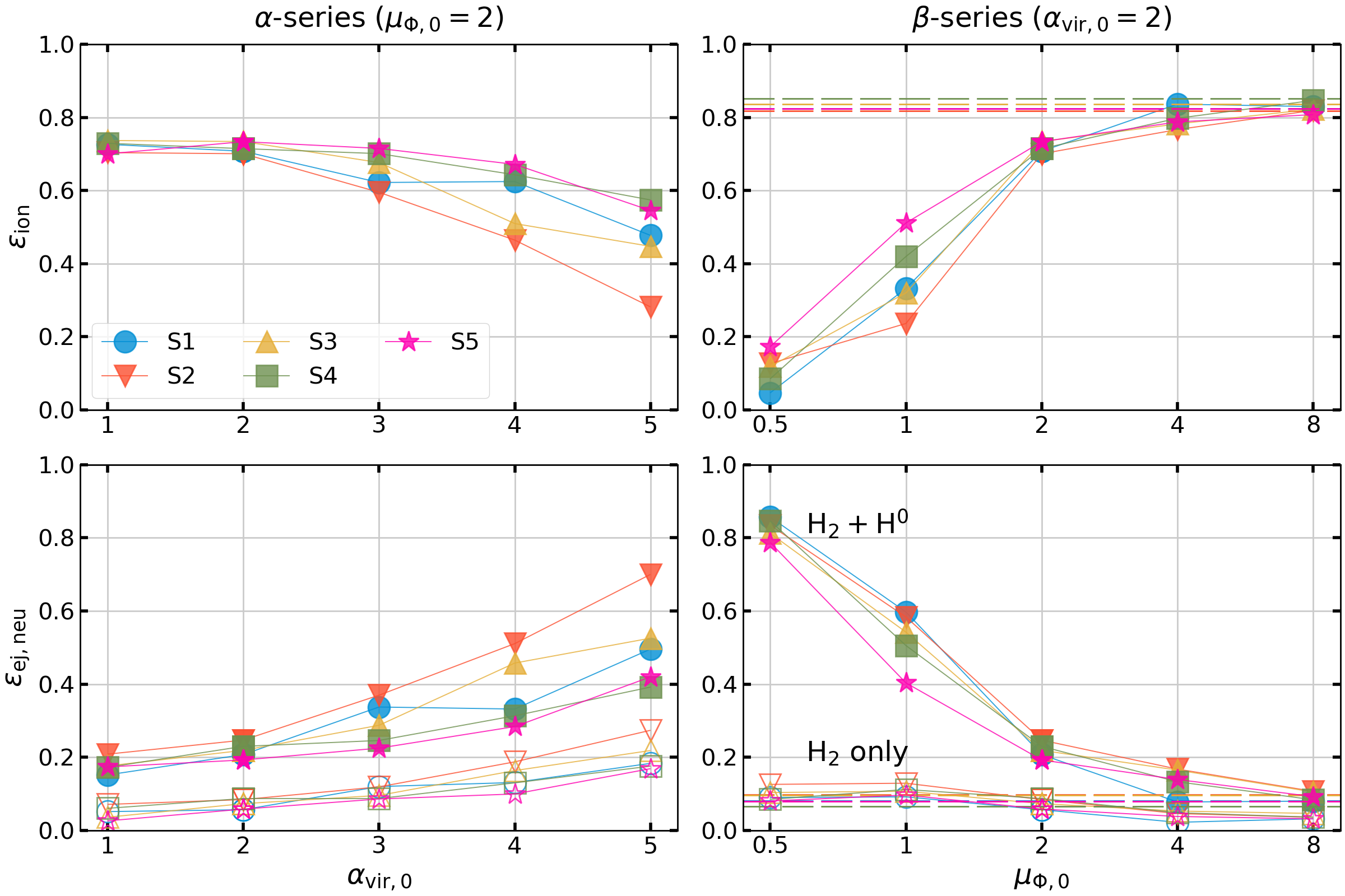
Figure 10: (Top) Fraction of initial cloud mass converted into ionized gas (photoevaporation efficiency; $\varepsilon_{\rm ion}$) and (bottom) ejected from the computational domain as neutrals (ejected neutral efficiency; $\varepsilon_{\rm ej,neu}$). The open symbols show the ejection efficiency of molecular gas. The left/right column shows results from the $\alpha$/$\beta$-series simulations, with different turbulent seed and unmagnetized models indicated as in Figure 9.

Clouds in our simulations are efficiently dispersed by UV radiation feedback, which converts the cold molecular gas that would otherwise form stars into atomic/ionized gas and drives outflows out of the computational domain. We define the photoevaporation efficiency ($\varepsilon_{\rm ion}$) as the fraction of the initial cloud mass turned into ionized gas, and the neutral ejection efficiency ($\varepsilon_{\rm ej,neu}$) as the fraction ejected from the simulation box in the molecular and atomic phases. Both $\varepsilon_{\rm ion}$ and $\varepsilon_{\rm ej,neu}$ are measured at the end of the simulation (see also Kim et al. 2018).

Figure 10 shows $\varepsilon_{\rm ion}$ (top) and $\varepsilon_{\rm ej,neu}$ (bottom) of the $\alpha$- (left) and $\beta$- (right) series models. The median/minimum/maximum values are listed in Table 2. Except for strongly magnetized ($\mu_{\Phi,0}\leq 1$) clouds, the mass loss is dominated by photoevaporation, consistent with the results of hydrodynamic simulations by Kim et al. (2018). In the $\alpha$-series models, as $\alpha_{\rm vir,0}$ increases from 1 to 5, the median value of $\varepsilon_{\rm ion}$ decreases from 73% to 48% while $\varepsilon_{\rm ej,neu}$ increases from 17% to 50%. This result can be understood as initially unbound clouds ejecting a larger amount of neutral gas by initial turbulence and having lower ionizing photon rate. In the $\beta$-series models, the median value of $\varepsilon_{\rm ion}$ is higher than $70\%$ for clouds with lower magnetization ($\mu_{\Phi,0}\geq 2$). In the magnetically subcritical (critical) case, however, only 13% (35%) of gas is photoevaporated by LyC photons and most of outflow mass is in the atomic phase. Although magnetically subcritical clouds have extended lifetime, the photoevaporation efficiency is low because of the low ionizing photon rate and magnetically confined H II region geometry. We also remark that outflows in magnetically subcritical clouds are unrealistically anisotropic; more than $\sim 80\%$ of the mass loss occurs along the $\hat{z}$ direction of the background magnetic field (through the vertical boundaries of the computational domain).

3.6 Timescales

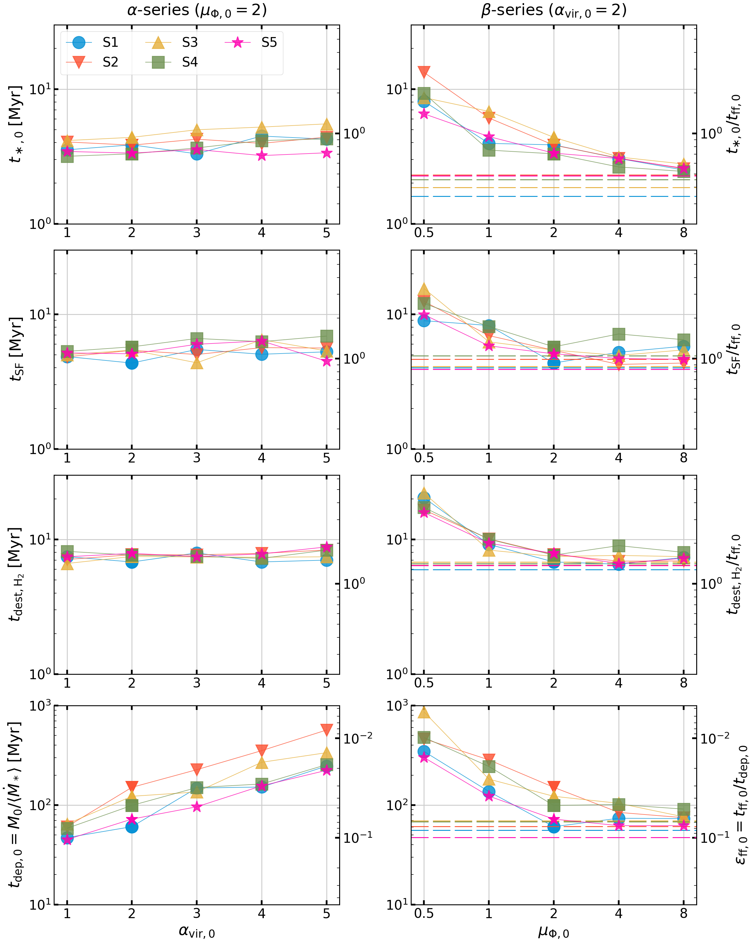
Figure 11: Evolutionary timescales with varying initial kinetic or magnetic energy or turbulence realization. From top to bottom, each row shows time of first star formation event $t_{*,0}$, duration of star formation $t_{\rm SF}=t_{*,90\%}-t_{*,0}$, timescale for cloud destruction $t_{\rm dest,H_{2}}=t_{\rm H_{2},5\%}-t_{*,0}$, and gas depletion time $t_{\rm dep,0}=M_{\rm 0}/\langle\dot{M}_{*}\rangle$. Left axes give times in Myr. Right axes (top three rows) show times in units of the initial freefall time $t_{\rm ff,0}=4.68\,{\rm Myr}$, while the bottom row shows the inverse, equivalent to the SFE per freefall time. The left/right column shows the $\alpha$/$\beta$-series simulations, with different turbulent seed and unmagnetized models indicated as in Figure 9.

Our simulations allow us to characterize several evolutionary timescales of GMCs dispersed by radiative feedback: the time of first star formation, timescales for star formation and cloud destruction, and the gas depletion time. Similar to the definition used by Kim et al. (2018), we define the duration of star formation as $t_{\rm SF}=t_{\rm*,90\%}-t_{\rm*,0}$. The cloud destruction time is defined as the time for the molecular gas mass to be reduced to $5\%$ of the initial cloud mass ($0.05M_{\rm 0}$), $t_{\rm dest,H_{2}}=t_{\rm H_{2},5\%}-t_{*,0}$. The gas depletion time is calculated using the initial cloud mass and the time-averaged SFR as $t_{\rm dep,0}=M_{\rm 0}/\langle\dot{M}_{*}\rangle$. This should be distinguished from the observed gas depletion time, based on instantaneous gas mass and SFR. We note that the “instantaneous” depletion time $M_{\rm gas}(t)/\dot{M}_{*}(t)$ will be close to $t_{\rm dep,0}$ if the SFR is relatively constant and only a small fraction of the mass has been dispersed by feedback; from Figure 3 and Figure 8, these conditions are generally satisfied for our simulations in the middle of the active star-forming phase. An inherent issue in observations, however, is how the SFR is measured; we return to this in Section 5.2. Finally, for the purposes of comparing to observations, we note that for constant SFR the mean age of an observed cluster in an actively star-forming cloud would be $t_{\rm SF}/3$. This assumes an equal number of stars in each age bin $\{t_{\rm SF}/N,2t_{\rm SF}/N,\cdots,t_{\rm SF}\}$ within a given cloud and equal representation of clouds at each age, so that the luminosity-weighted average age of clusters would be $t_{\rm SF}(N+2)/(3N)$.

Figure 11 shows, from top to bottom, $t_{*,0}$, $t_{\rm SF}$, $t_{\rm dest,H_{2}}$, $t_{\rm dep,0}$ of the $\alpha$- (left) and $\beta$-series (right) models. Results for all turbulence realizations (labeled by seed) are shown separately; median, minimum, and maximum values for each model are summarized in Table 2. In the $\alpha$-series models, the median value of $t_{*,0}$ ranges from $3.5\,{\rm Myr}$ to $4.3\,{\rm Myr}$, equivalent to $0.8-0.9t_{\rm ff,0}$, increasing only weakly with $\alpha_{\rm vir,0}$. The duration of star formation is also roughly constant (slightly increasing with $\alpha_{\rm vir,0}$) at $t_{\rm SF}\sim 5$–$6\,{\rm Myr}$, which is $\sim 1.1$–$1.3t_{\rm ff,0}$. Cloud destruction occurs within $\sim 1.6$–$1.8t_{\rm ff,0}$, a few Myrs after $t_{*,90\%}$, consistent with the results of hydrodynamic simulations in Kim et al. (2018).

In the $\beta$-series models, $t_{*,0}$ systematically increases with decreasing $\mu_{\Phi,0}$ while $t_{\rm SF}$ and $t_{\rm dest,H_{2}}$, have mild variations with $\mu_{\Phi,0}$ for $\mu_{\Phi,0}\gtrsim 2$, but all timescales become significantly longer in the magnetically critical and especially subcritical cases. For example, the model A2B05S4 has $t_{*,0}=9.3\,{\rm Myr}$, $t_{\rm SF}=12.0\,{\rm Myr}$, and $t_{\rm dest,H_{2}}=17.3\,{\rm Myr}$ (see also Figure 3(g)).

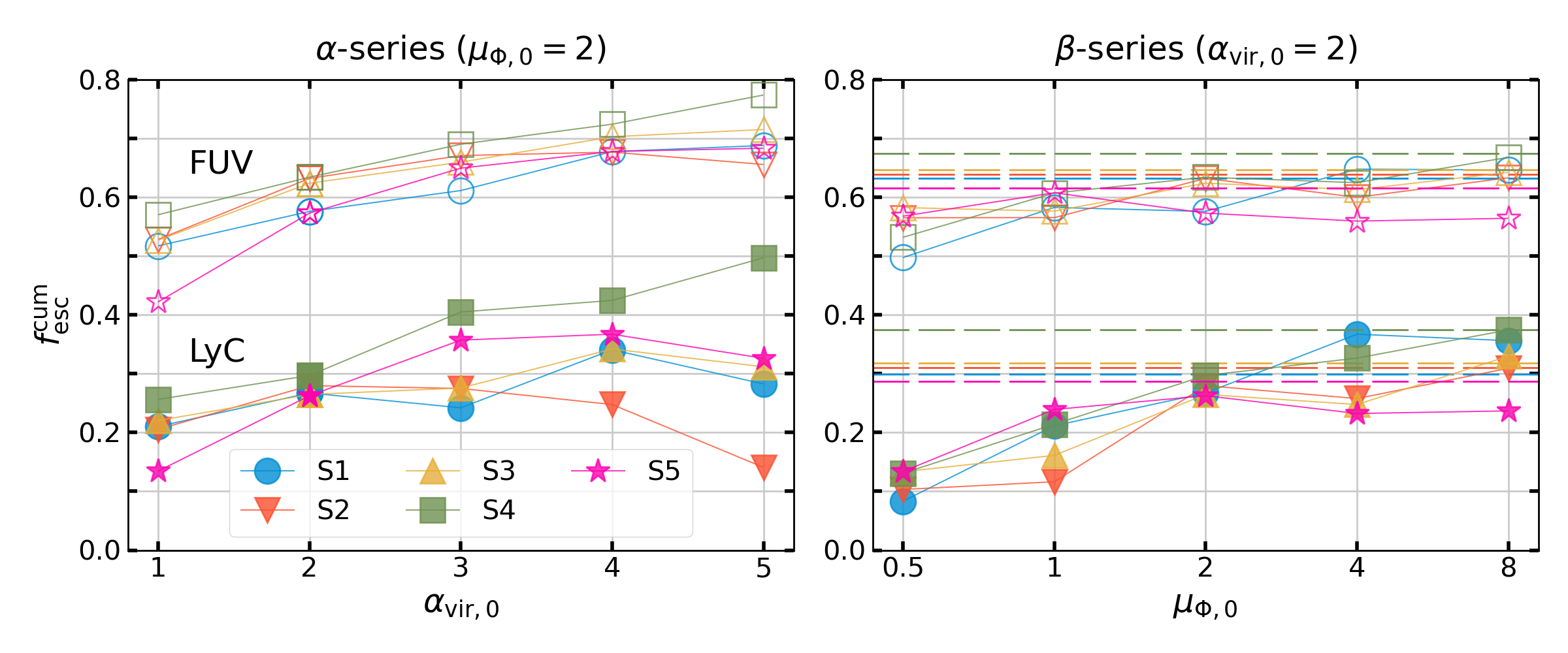
Figure 12: Cumulative escape fractions of LyC and FUV radiation for our $\alpha$-series (left) and $\beta$-series models (right). Different turbulent seed and unmagnetized models are indicated as in Figure 9.

The depletion time $t_{\rm dep,0}$ systematically increases with increasing $\alpha_{\rm vir,0}$, with median values ranging over $58$–$255\,{\rm Myr}$. The median depletion time also increases from $61$–$464\,{\rm Myr}$ from unmagnetized to subcritically-magnetized models. The ratio $t_{\rm ff,0}/t_{\rm dep,0}$ is equivalent to the SFE per initial freefall time of the cloud (we shall introduce the notation $\varepsilon_{\rm ff,0}$ for this ratio in Equation (33)). For our models, the median value of $t_{\rm ff,0}/t_{\rm dep,0}$ increases from 1.8% to 8.0% as $\alpha_{\rm vir,0}$ decreases, and from 1.0% to 7.7% as $\mu_{\Phi,0}$ increases. We further discuss how our results on efficiency per freefall time relate to theoretical models and observations in Section 5.

3.7 Escape Fraction of Radiation

Figure 12 shows the cumulative escape fractions of LyC and FUV radiation measured at the end of simulations (see also Table 2). Because neutral hydrogen acts as an additional source of opacity for ionizing radiation and most of LyC photons are emitted before the cloud destruction, the escape fraction of LyC radiation is smaller than that of FUV radiation.

In the $\alpha$-series, median values of $f_{\rm esc,LyC}^{\rm cum}$ are in the range $21$–$34\%$, generally increasing with $\alpha_{\rm vir,0}$, although there is a significant variation with random seeds at large $\alpha_{\rm vir,0}$. In the $\beta$-series, $f_{\rm esc,LyC}^{\rm cum}$ increases with decreasing magnetic field strength, with medians in the range $13$–$33\%$. For point radiation sources, the escape fraction is determined by the solid-angle PDF of the optical depth as seen from the source and is higher if the width of the PDF is higher (Safarzadeh & Scannapieco, 2016; Kim et al., 2019b). Therefore, the trend in the $\beta$-series is a result of the reduced gas compressibility and the reduced width of the column density PDF in strongly magnetized clouds (e.g., Ostriker et al., 2001).

In all of our models, $f_{\rm esc,LyC}^{\rm cum}$ measured at $t^{\prime}=3\,{\rm Myr}$ is only $\sim 2$–$10\%$. In contrast, the hydrodynamic simulations of Kim et al. (2019b) found that $f_{\rm esc,LyC}^{\rm cum}=30\%$ at $t^{\prime}=3\,{\rm Myr}$ for the same cloud with $M_{\rm 0}=10^{5}\,M_{\odot}$, $R_{\rm 0}=20\,{\rm pc}$, ${\rm seed}=1$, $\mu_{\Phi,0}=\infty$. This discrepancy is likely due to different treatments of the ionizing photon production rate per stellar mass in the two simulations. In the present simulations, $\Psi_{\rm LyC}$ decreases with time and $\Psi_{\rm LyC}(t_{\rm age}=3\,{\rm Myr})\approx 0.5\Psi_{\rm LyC}(0)$; the cumulative value is heavily weighted by values at early times when $f_{\rm esc,LyC}\ll 1$. In contrast, the conversion factor adopted by Kim et al. (2019b) was constant with time, but depended on the total cluster mass to account for the effects of poor sampling of the IMF at the high mass end. This effectively made the LyC photon production rate per unit mass lower at the earliest times (when $M_{*,\rm total}\lesssim 10^{3}$) compared to later time. Thus, the luminosity-weighted escape fraction was more heavily weighted to later times when photons escape more easily.

4 Virial Ratios

The virial theorem

$$\frac{1}{2}\ddot{I}+\frac{1}{2}\frac{\mathrm{d}}{\mathrm{d}t}\int\rho r^{2}\bm{v}\cdot d\bm{S}=2(\mathcal{T}-\mathcal{T}_{\rm s})+(\mathcal{B}-\mathcal{B}_{\rm s})+\mathcal{U}$$ (20)

describes the rate of change of a gaseous system’s moment of inertia ($I=\int\rho r^{2}\mathrm{d}V$) due to kinetic and thermal ($\mathcal{T}=\mathcal{T}_{\rm kin}+\mathcal{T}_{\rm thm}$), magnetic ($\mathcal{B}$), and gravitational ($\mathcal{U}$) energies associated with it (e.g., McKee & Zweibel, 1992).

The terms with subscript “s” are integrals involving Reynolds and Maxwell stresses over a bounding surface that fully encloses the system of interest, given by

$$2\mathcal{T}_{\rm s}=\int_{S}\bm{r}\cdot\left(P\mathbb{1}+\rho\bm{v}\bm{v}\right)\cdot d\bm{S}$$ (21)

and

$$\mathcal{B}_{\rm s}=-\frac{1}{4\pi}\int_{S}\bm{r}\cdot\left(\bm{B}\bm{B}-(B^{2}/2)\mathbb{1}\right)\cdot d\bm{S}.$$ (22)

If the surface stresses are isotropic, these may be evaluated as $2\mathcal{T}_{\rm s}=3[P+\rho\sigma_{\rm 1d}^{2}]_{\rm s}V$ and $\mathcal{B}_{\rm s}=3[B_{\rm 1d}^{2}/(8\pi)]_{\rm s}V$, where the subscript “s” indicates an average over the bounding surface, $V$ is the enclosed volume and “1d” denotes the component along any single direction. Thus, $2\mathcal{T}_{\rm s}$ corresponds to what would be twice the sum of “ambient” thermal and kinetic energy within $V$, while $\mathcal{B}_{\rm s}$ corresponds to what would be the “ambient” magnetic energy within $V$. Equivalently, $(2\mathcal{T}_{\rm s}+\mathcal{B}_{\rm s})/V=3P_{\rm amb}$, where the total ambient pressure $P_{\rm amb}$ includes thermal, turbulent, and magnetic terms.

The virial theorem has been widely invoked to study cloud stucture, stability, and evolution (e.g., Zweibel, 1990; Bertoldi & McKee, 1992; McKee & Zweibel, 1992; Shu, 1992; McKee, 1999; Ballesteros-Paredes et al., 1999; Dib et al., 2007; Ballesteros-Paredes et al., 2009) and to obtain mass estimates for molecular clouds (e.g., Solomon et al., 1987; Bolatto et al., 2008).

Some useful insights can be obtained by considering simple limiting cases. When Equation (20) is averaged over an ensemble of turbulent clouds in different microstates, the terms on the left hand side would average out to zero. In weakly self-gravitating cases, $\mathcal{T}\approx\mathcal{T}_{\rm s}$ and $\mathcal{B}\approx\mathcal{B}_{\rm s}$, with one (or both) $\gg|\mathcal{U}|$. In this situation, molecular clouds would just represent overdense, UV-shielded parts of the turbulent ISM, with internal terms balancing the surface terms; the ambient material could be either diffuse molecular or atomic gas. Indeed, the study of Schruba et al. (2019) suggests that there are both atomic-dominated and molecule-dominated cases with $\mathcal{T}_{\rm s}\approx\mathcal{T}\gg|\mathcal{U}|$.

More generally, for an ensemble of clouds where the time-dependent terms are zero, we would have

$$\frac{2\langle\mathcal{T}\rangle}{\langle{|\mathcal{U}|}\rangle}=\frac{\langle\mathcal{T}\rangle}{\langle\mathcal{T}-\mathcal{T}_{\rm s}\rangle+\langle\mathcal{B}-\mathcal{B}_{\rm s}\rangle/2}.$$ (23)

If the magnetic terms are individually small, or if the surface and volume magnetic terms are comparable (which would be true for a uniform magnetic field), this ratio would be greater than unity. Alternatively, if surface terms $\mathcal{T}_{\rm s}$ and $\mathcal{B}_{\rm s}$ are small compared to corresponding volume terms, this ratio would be less than unity. Thus, while “virialized” is often taken as synonymous with having $2\mathcal{T}/|\mathcal{U}|\approx 1$, this is not true in general (and does not appear to be satisfied for observed molecular clouds in many environments – see Schruba et al., 2019). Rather, for an ensemble of clouds in statistical equilibrium (some forming and others dispersing) we would expect

$$1\approx\frac{2\langle\mathcal{T}-\mathcal{T}_{\rm s}\rangle+\langle\mathcal{B}-\mathcal{B}_{\rm s}\rangle}{\langle|\mathcal{U}|\rangle}$$ (24)

or

$$\frac{2\langle\mathcal{T}\rangle}{\langle|\mathcal{U}|\rangle}\left(1+\frac{\langle\mathcal{B}\rangle}{2\langle\mathcal{T}\rangle}\right)\approx 1+\frac{2\langle\mathcal{T}_{s}\rangle+\langle\mathcal{B}_{s}\rangle}{\langle|\mathcal{U}|\rangle}\,.$$ (25)

The analogous expressions without angle brackets would also be true for an individual cloud if the “acceleration” terms on the left-hand side of Equation (20) are small.

The ratios $2\langle\mathcal{T}\rangle/\langle|\mathcal{U}|\rangle$ and $(2\langle\mathcal{T}_{s}\rangle+\langle\mathcal{B}_{s}\rangle)/\langle|\mathcal{U}|\rangle$ in Equation (25) can be estimated observationally based on the measurements of cloud-scale internal pressure and large-scale pressure that is in balance with vertical weight of the ISM. First, the ratio $2\langle\mathcal{T}\rangle/\langle|\mathcal{U}|\rangle$ is proportional to the ratio between the velocity dispersion squared and the gravitational potential of molecular gas, both averaged over cloud populations weighted by the CO intensity. It is also proportional to the ratio between the internal (turbulent plus thermal) pressure and self-gravitational weight of molecular gas (e.g., Schruba et al., 2019). Second, to the extent that surface stresses are isotropic when ensemble averaged, the surface term $\langle 2\mathcal{T}_{\rm s}+\mathcal{B}_{\rm s}\rangle$ is equal to $3V\langle P_{\rm amb}\rangle$ (see Equations (21)–(22) and following). Numerical simulations show that the total ambient pressure at the midplane is generally in good agreement with vertical dynamical equilibrium predictions for the large-scale ISM, so standard expressions based on the gas surface density and the stellar density may be used to estimate $P_{\rm amb}$ (e.g., Kim et al., 2013; Kim & Ostriker, 2015). Given the knowledge of these quantities, one may infer the fractional contribution from magnetic support on cloud sales, $\mathcal{B}/(2\mathcal{T})$ or $\mathcal{B}/|\mathcal{U}|$.

While it is observationally very difficult, if not impossible, to determine the individual terms in Equation (20) with precision (e.g, Singh et al., 2019), observers have traditionally employed the simple kinetic virial parameter $\alpha_{\rm vir}=5\sigma_{\rm 1d}^{2}R/(GM)$ based on estimates of size, velocity dispersion, and mass to assess whether a cloud is gravitationally bound ($\alpha_{\rm vir}<2$) or in virial equilibrium ($\alpha_{\rm vir}\approx 1$). Strictly speaking, these diagnostics using $\alpha_{\rm vir}$ apply to a steady-state homogeneous, spherical, non-magnetized cloud with no external forces acting on it. In particular, simple approaches treat clouds as isolated, while in reality GMCs are often in close proximity to each other and/or surrounded by cold H I envelopes with significant mass. The former would reduce the magnitude of the gravitational energy because the effective zero of the gravitational potential lies near clouds rather than at infinite distance, while the latter would make the effective potential deeper (e.g., Ballesteros-Paredes, 2006). By analyzing the dynamical state of structures found in kpc-scale simulations of the multiphase, star-forming ISM with self-consistent star formation and supernova feedback, Mao et al. (2020) found that $\alpha_{\rm vir}$ is often inadequate as a measure of the gravitational boundedness of a structure, because tidal gravity, magnetic terms, and other effects can be large.

While in the present simulations there are no tidal forces, our model clouds otherwise have quite realistic physics and very high resolution. It is therefore interesting to test how well the simple estimate $\alpha_{\rm vir}$ represents the true boundedness of our simulated clouds. To do this, we directly measure the virial parameter accounting for kinetic, thermal, and magnetic energies and compare with $\alpha_{\rm vir}$ computed via the traditional estimate.

We calculate the energies of the neutral gas in the cloud as

$$\mathcal{T}_{\rm kin}=\frac{1}{2}\int\rho v^{2}\Theta\mathrm{d}V\,,$$ (26)

$$\mathcal{T}_{\rm thm}=\frac{3}{2}\int P\Theta\mathrm{d}V\,,$$ (27)

$$\mathcal{B}=\frac{1}{8\pi}\int B^{2}\Theta\mathrm{d}V\,,$$ (28)

$$\mathcal{U}=-\int\rho\bm{r}\cdot\nabla\Phi\Theta\mathrm{d}V\,.$$ (29)

(e.g., McKee & Zweibel, 1992). The gravitational potential $\Phi$ in Equation (29) includes contributions from not only the neutral cloud gas but also ionized gas and stars in the computational domain. Because $\Phi$ includes “external” terms, we cannot re-express $\mathcal{U}$ as $-(1/2)\int\rho\Phi dV$; the latter expression would only apply if we were solely considering the self-gravitational energy of the gas cloud.

In the analysis of our simulations, we shall ignore the surface terms $\mathcal{T}_{\rm s}$ and $\mathcal{B}_{\rm s}$. Given the low density and high temperature of the ambient medium in our simulations, in fact $\mathcal{T}_{\rm kin,s}$ is much smaller than $\mathcal{T}_{\rm kin}$ and $\mathcal{T}_{\rm thm,s}$ is comparable to $\mathcal{T}_{\rm thm}$.

In principle, the magnetic energy associated with the cloud $\mathcal{B}-\mathcal{B}_{\rm s}$ can be calculated as the difference between the total magnetic energy of the cloud and magnetic energy of the ambient field in the absence of the cloud (McKee & Zweibel, 1992). However, our simulations impose an initially uniform magnetic field rather than e.g., some kind of hourglass geometry (which we avoided since it would be arbitrary). As such, the ambient field strength can be larger than realistic values. While this does not affect dynamics within the cloud itself, it would imply an unrealistically large measured $\mathcal{B}_{\rm s}$ compared to $\mathcal{B}$. If we had begun with a larger-scale simulation that followed cloud formation, the ambient magnetic field would be lower than the cloud value, and $\mathcal{B}_{\rm s}$ would be small compared to $\mathcal{B}$. In particular, if magnetic flux is conserved in the formation of a cloud of size $R_{\rm cl}$ from a region of crossection $\sim R_{d}^{2}$ in the diffuse ISM, the volume magnetic term would exceed the surface term by a factor of order $R_{\rm d}/R_{\rm cl}\gg 1$. Therefore, our $\mathcal{B}$ can be considered as an approximation of (and an upper limit to) the true magnetic term.

With the above definitions, the more exact equivalent of the traditional kinetic virial parameter defined (for the initial cloud) in Equation (15) is

$$\tilde{\alpha}_{\rm vir}\equiv\frac{2\mathcal{T}_{\rm kin}}{|{\cal U}|};$$ (30)

we use the tilde to emphasize the distinction.

The third row in Figure 5 plots the evolution of kinetic, thermal, magnetic, and gravitational energies of the cloud in models A2B2S4, A5B2S4, and A2B05S4. In the fiducial model, the magnitude of the gravitational energy $\mathcal{U}$ remains very close to the initial value $3GM_{\rm 0}^{2}/(5R_{\rm 0})$ at early times. At late times ($t\gtrsim 5\,{\rm Myr}$), it begins to decrease as gas is photoevaporated and dispersed. A naive estimate $3GM_{\rm neu}^{2}/(5R)$ for the gravitational energy using the half-mass radius ($R=2^{1/3}R_{50\%}$) is also shown using a blue dashed curve; the true gravitational energy is larger than this at late times. This is because the simple estimate ignores substructure in the mass distribution, which is characterized by a few widely-separated clusters of gas clumps (which themselves contain closely packed dense cores), leading to the overestimation of the effective size of the system at late times as the cloud disperses.

The evolution of the kinetic energy $\mathcal{T}_{\rm kin}$ follows that of the velocity dispersion (second row in Figure 5), although the increase after $t\sim 5\,{\rm Myr}$ is less significant due to mass loss. The magnetic energy is $2GM_{0}^{2}/(3R_{0}\mu_{\Phi,0}^{2})$ initially, then increases slightly due to turbulence-induced magnetic fields, and saturates at a level that is about half the initial gravitational energy, until it decreases due to gas dispersal at late times. The thermal energy is unimportant at early times, but later becomes comparable to $\mathcal{B}$ and $|\mathcal{U}|$ due to the FUV heating.

The other two models show similar evolutionary trends for gravitational and kinetic terms. It is worth noting that $|\mathcal{U}|$ in ${\tt A5B2S4}$ decreases starting from $t=0$ due to the initial expansion of the unbound cloud. The magnetic energy in the subcritical model ${\tt A2B05S4}$ is larger than the other terms throughout the simulation.

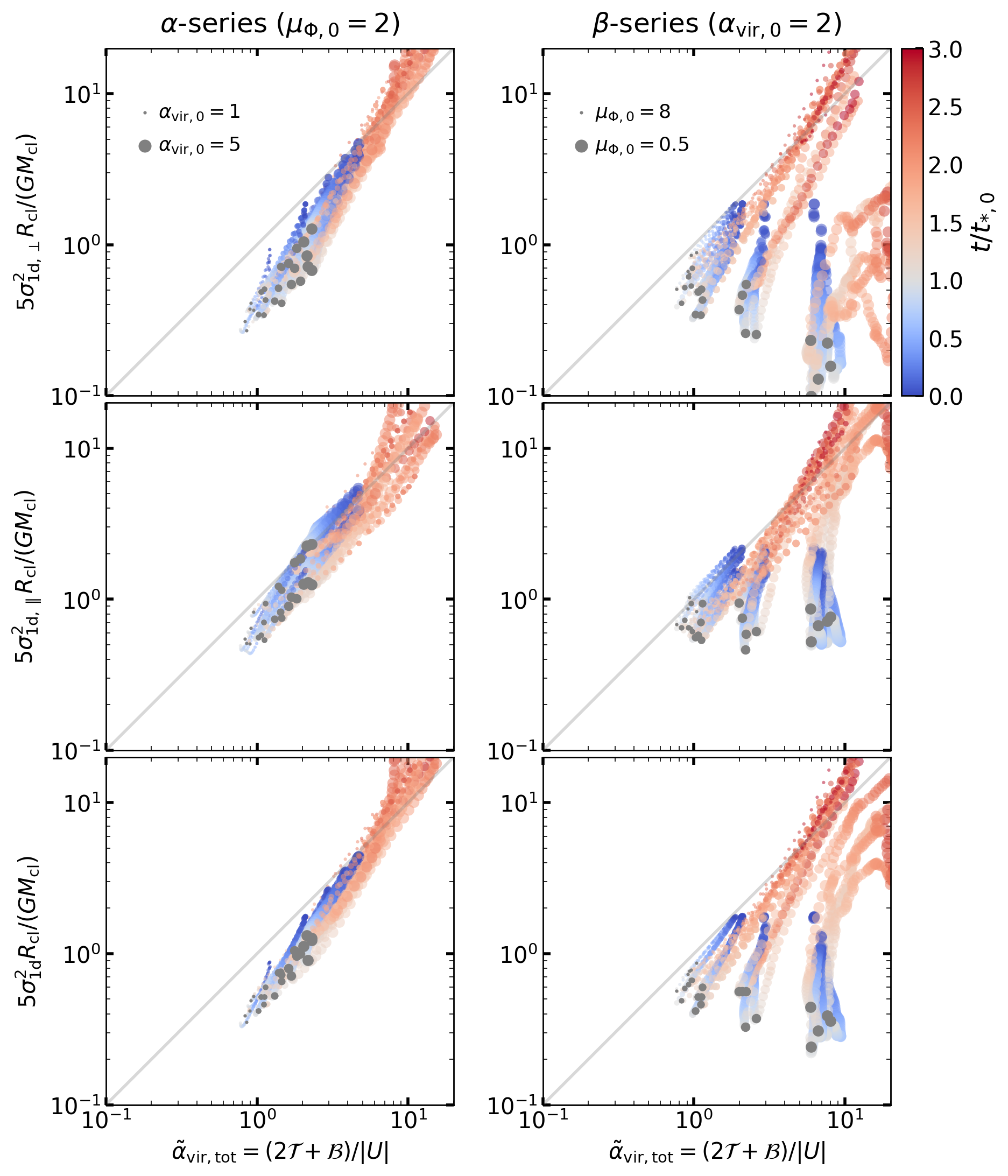
Figure 13: Comparison of the virial ratio $\tilde{\alpha}_{\rm vir,tot}=(2\mathcal{T}+\mathcal{B})/|\mathcal{U}|$ and the traditional kinetic virial parameter defined as $\alpha_{\rm vir}=5\sigma_{\rm 1d}^{2}R/(5M_{\rm neu})$ in the $\alpha$-series (left) and $\beta$-series (right) models. Each circle represents one snapshot and the color indicates the time of the snapshot normalized by the time of the first star formation. The grey circles mark values at $t=t_{*,0}$. The size of circles increases with increasing $\alpha_{\rm vir,0}$ and $B_{z,0}$ (decreasing $\mu_{\Phi,0}$). Rows show the traditional $\alpha_{\rm vir}$ calculated with velocity dispersion perpendicular (top) and parallel (middle) to the background magnetic field and averaged along all three Cartesian axes (bottom).

In the fourth row of Figure 5, we show as gray lines the “observed” virial parameter $\alpha_{\rm vir}$ computed from the instantaneous $M_{\rm neu}$ and $R=2^{1/3}R_{50\%}$, and three different measures of the velocity dispersion: $\sigma_{\rm 1d,\perp}$, $\sigma_{\rm 1d,\parallel}$, and $\sigma_{\rm 1d}$. We compare to the ratio $\tilde{\alpha}_{\rm vir}=2\mathcal{T}_{\rm kin}/|\mathcal{U}|$ (cyan). The kinetic virial parameter $\alpha_{\rm vir}=5\sigma_{\rm 1d}^{2}R/(GM_{\rm neu})$ (solid gray) agrees very well with $\tilde{\alpha}_{\rm vir}=2\mathcal{T}_{\rm kin}/|\mathcal{U}|$ at early times, but becomes larger than $\tilde{\alpha}_{\rm vir}$ when cloud disruption is underway, as the true gravitational binding energy is larger than the simple estimate $3GM_{\rm neu}^{2}/(5R)$.

Because clouds are supported jointly by thermal energy, turbulence, and magnetic fields, it is natural to consider virial parameters including additional terms. The virial parameter including both nonthermal and thermal gas motions is $2\mathcal{T}/|\mathcal{U}|$. The virial parameter accounting for the total energy is

$$\tilde{\alpha}_{\rm vir,tot}=\frac{2\mathcal{T}+\mathcal{B}}{|\mathcal{U}|}\,.$$ (31)

The time evolution of $2\mathcal{T}/|\mathcal{U}|$ (purple) and $(2\mathcal{T}+\mathcal{B})/|\mathcal{U}|$ (black) are plotted in the bottom row of Figure 5. The thermal terms do not make a large difference, but the magnetic term can lead to a factor of two increase in $\tilde{\alpha}_{\rm vir,tot}$ compared to $\tilde{\alpha}_{\rm vir}$, or even more for the most strongly magnetized model.

The scatter plots in Figure 13 show the relationship between the traditional kinetic virial parameter estimate ($\alpha_{\rm vir}$) and total virial ratio ($\tilde{\alpha}_{\rm vir,tot}$) for all of the simulation snapshots taken before $t_{*,90\%}$ in the $\alpha$- (left) and $\beta$-series (right) models. From top to bottom, the ordinate shows the kinetic virial parameter computed using $\sigma_{\rm 1d,\perp}$, $\sigma_{\rm 1d,\parallel}$, and $\sigma_{\rm 1d}$. The symbols are colored by time normalized to $t_{*,0}$. Grey dots mark the values at $t=t_{*,0}$.

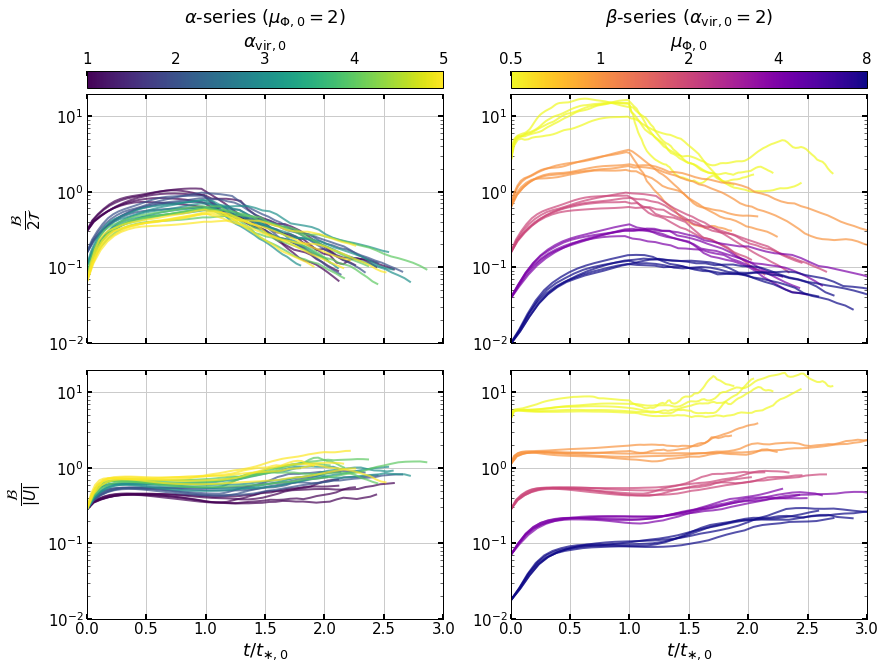
Figure 14: Time evolution of the ratio of the magnetic energy ($\mathcal{B}$) to twice the kinetic energy ($2\mathcal{T}$; top) and to the gravitational ($|\mathcal{U}|$) energy until $t_{*,90\%}$ in all of the $\alpha$- (left) and $\beta$-series (right) models. Models with lighter colors have stronger initial turbulence ($\alpha$-series) or magnetic field strength ($\beta$-series). The time is normalized by the time of first star formation $t_{*,0}$.

Except for the strongly magnetized models, $\tilde{\alpha}_{\rm vir,tot}$ initially decreases with time due to the decay of turbulence, and then turns around after the onset of radiative feedback. Remarkably, the total virial parameter at $t=t_{*,0}$ in the $\alpha$-series falls in a fairly narrow range $\tilde{\alpha}_{\rm vir,tot}\sim 0.9$–$2.1$, suggesting that small-scale collapse starts when the cloud reaches a near-virial state. Except for the subcritical clouds A2B05, $\tilde{\alpha}_{\rm vir,tot}\sim 0.9$–$2.2$ at $t=t_{*,0}$ in the $\beta$-series as well. In contrast, the magnetically subcritical clouds (A2B05) remain globally unbound throughout their evolution.

The results of the $\alpha$-series models suggest that, for moderate magnetic field strength ($\mu_{\Phi,0}=2$), $\alpha_{\rm vir}$ can slightly underestimate or more significantly overestimate the true gravitational boundedness depending on the relative orientation between the mean magnetic field and the observer’s line of sight. The bottom panels of Figure 13 suggest that, even with the correct estimate of kinetic energy, the kinetic virial parameter would systematically overrate the boundedness due to the neglect of magnetic support. We find that the median value of the ratio $\tilde{\alpha}_{\rm vir,tot}/\alpha_{\rm vir}$ for the $\alpha$-series ranges between $1.48$–$1.65$.

The results of the $\beta$-series models (the bottom right panel in Figure 5 and the top right panel in Figure 13) suggest that the use of the traditional kinetic virial parameter can significantly underestimate the kinetic energy in magnetically critical and subcritical clouds when the line of sight is orthogonal to the field direction. Still, except for extreme magnetizations and orientations, the traditional $\alpha_{\rm vir}$ estimates boundedness within a factor of $\sim 2$. We find that the median value of the ratio $\tilde{\alpha}_{\rm vir,tot}/\alpha_{\rm vir}$ for the $\beta$-series except for A2B05 is $1.07$–$1.94$. For the magnetically subcritical clouds, the median value of $\tilde{\alpha}_{\rm vir,tot}/\alpha_{\rm vir}$ is $5.61$.

To quantify the relative importance of magnetic support, in Figure 14 we show the time evolution of the magnetic energy divided by twice the kinetic (top) or the gravitational (bottom) energy in the $\alpha$- (left) and $\beta$-series (right) models. In all models, the ratio $\mathcal{B}/(2\mathcal{T})$ increases at early times (due to kinetic turbulence decay and magnetic turbulence growth), and decreases at late times due to feedback-driven dispersal; the ratio $\mathcal{B}/|\mathcal{U}|$ exhibits a mild temporal variation (see also third row of Figure 5). In the $\alpha$-series models, $\mathcal{B}/(2\mathcal{T})$ ($\mathcal{B}/|\mathcal{U}|$) falls in a range $\sim 0.22$–$1.10$ ($0.34$–$1.09$) for $0.5\leq t/t_{*,0}\leq 1.5$. The right panels based on the $\beta$-series show that the importance of magnetic support widely varies depending on the initial magnetic field strength; $\mathcal{B}/(2\mathcal{T})$ can be as large (small) as 17 (0.07) in strongly (weakly) magnetized clouds for $0.5\leq t/t_{*,0}\leq 1.5$.

We emphasize that the above results are for isolated clouds; tidal forces will reduce the gravitational energy, which would increase $\tilde{\alpha}_{\rm vir,tot}$. This would enhance the discrepancy between the traditional virial estimate and the true boundedness shown in the bottom panels of Figure 13 and the ratio $\mathcal{B}/|\mathcal{U}|$ shown in the bottom panels of Figure 14.

5 SFE per Freefall Time

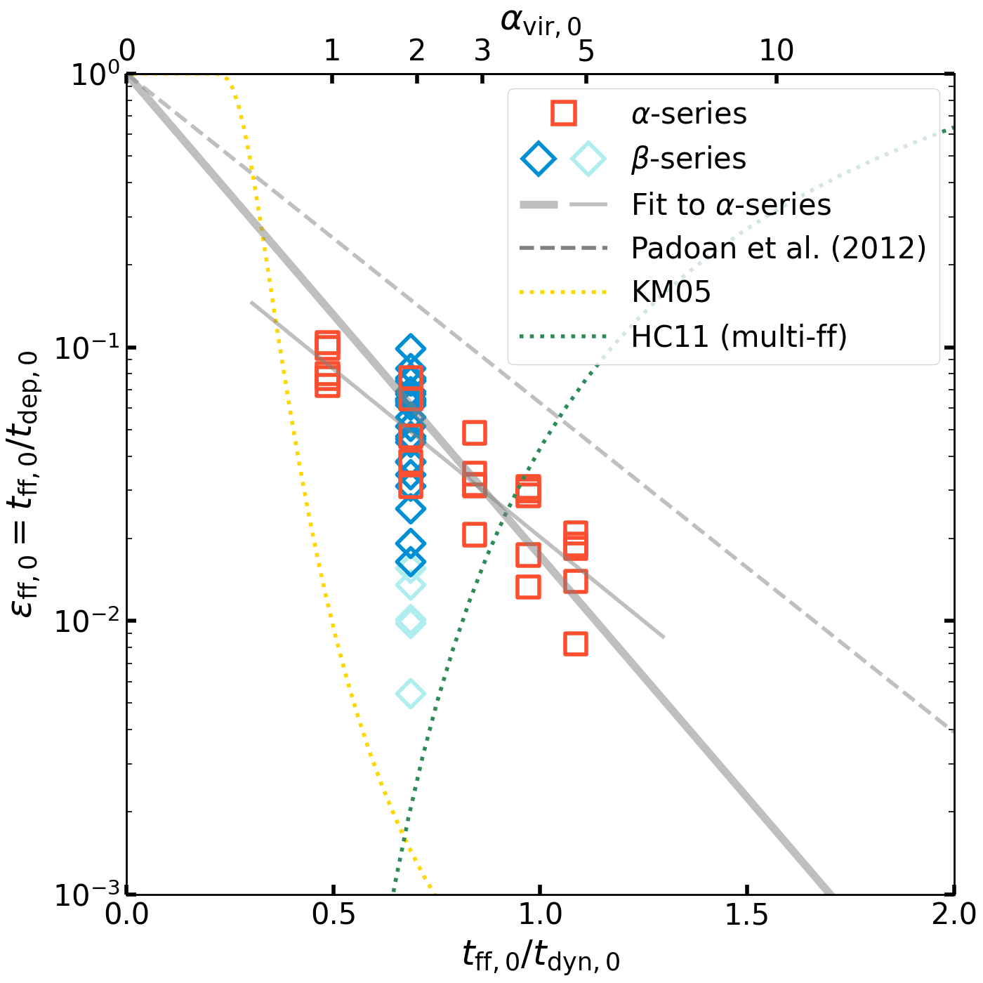
Figure 15: Time-averaged SFE per free fall time defined as $\varepsilon_{\rm ff,0}=t_{\rm ff,0}\langle\dot{M}_{*}\rangle/M_{\rm 0}=t_{\rm ff,0}/t_{\rm dep,0}$ as a function of $\alpha_{\rm vir,0}$ (top $x$-axis) or the ratio between the initial freefall and dynamical times (bottom $x$-axis) in the $\alpha$-series (red squares) and the $\beta$-series (diamonds in dark blue for critical critical/supercritical and light blue for subcritical) models. The numerical result $\exp(-1.6\sqrt{3}t_{\rm ff,0}/t_{\rm dyn,0})$ found by Padoan et al. (2012) is shown as a gray dashed line. The thick gray solid line shows the fit to the $\alpha$-series simulations $\varepsilon_{\rm ff,0}=\exp(-4.06t_{\rm ff,0}/t_{\rm dyn,0})$. The thin gray solid line segment shows the results of a two-parameter fit $\varepsilon_{\rm ff,0}=0.34\exp(-2.83t_{\rm ff,0}/t_{\rm dyn,0})$. The dotted lines show the predictions from the Krumholz & McKee and Hennebelle & Chabrier analytic models (see text for details).

The freefall time $t_{\rm ff}=\sqrt{3\pi/(32G\rho)}$ is a natural characteristic timescale in a self-gravitating gaseous system, representing the shortest possible timescale for gravitational collapse at a given mean density. In common practice, the SFR is expressed as

$$\dot{M}_{*}\equiv\varepsilon_{\rm ff}\frac{M_{\rm gas}}{t_{\rm ff}},$$ (32)

which defines the SFE per freefall time $\varepsilon_{\rm ff}$; the freefall time is evaluated at the mean density of the system (e.g., Krumholz & McKee, 2005). Since the SFR is also defined in terms of the depletion time, $\dot{M}_{*}\equiv M_{\rm gas}/t_{\rm dep}$, these are related by $\varepsilon_{\rm ff}=t_{\rm ff}/t_{\rm dep}$. A cloud collapsing under its own gravity without any hindrance would form stars at maximal efficiency ($\varepsilon_{\rm ff}\approx 1$, $t_{\rm dep}\approx t_{\rm ff}$). A wealth of observational studies however suggest that both galactic and cloud-scale star formation proceeds much slower than the freefall rate ($\varepsilon_{\rm ff}\ll 1$ or $t_{\rm dep}\gg t_{\rm ff}$) (e.g., Zuckerman & Evans, 1974; Williams & McKee, 1997; Krumholz & Tan, 2007; Kennicutt & Evans, 2012; Evans et al., 2014; Lee et al., 2016; Barnes et al., 2017; Leroy et al., 2017; Ochsendorf et al., 2017; Utomo et al., 2018).

In our simulations, we measure the SFE per freefall time using the mass and freefall time of the cloud at $t=0$ and the time-averaged SFR $\langle\dot{M}_{*}\rangle$ as

$$\varepsilon_{\rm ff,0}=t_{\rm ff,0}\frac{\langle\dot{M}_{*}\rangle}{M_{\rm 0}}=\frac{t_{\rm ff,0}}{t_{\rm dep,0}}\,.$$ (33)

This is similar to the approach adopted by Padoan et al. (2012); Raskutti et al. (2016). Since $t_{\rm ff,0}$ is the same ($4.68\,{\rm Myr}$) for all of the present models, $t_{\rm dep,0}$ and $\varepsilon_{\rm ff,0}$ are inversely proportional to each other.

The right $y$-axes in the bottom row of Figure 11 indicates that $\varepsilon_{\rm ff,0}$ ranges between $0.008$ and $0.1$ in the $\alpha$-series and between $0.006$ and $0.1$ in the $\beta$-series, with scatter of $0.3$–$0.5\,{\rm dex}$ for each model. Note that the ratio between $\varepsilon_{\rm*}$ and $\varepsilon_{\rm ff,0}$ corresponds to the duration of star formation in units of $t_{\rm ff,0}$ (second row in Figure 11), which is in the range $\sim 1$–$2$ (except for the subcritical models).

Our simulations show that $\varepsilon_{\rm ff,0}$ decreases when the virial parameter increases, which is qualitatively consistent with some previous work. In the rest of this section, we study more quantitatively the relationship between the SFE per freefall time and the virial parameter in comparison to other simulations, theoretical models, and observations.

5.1 Comparison with Simulations and Theory

In Figure 15, we plot $\varepsilon_{\rm ff,0}$ of all models against the ratio $t_{\rm ff,0}/t_{\rm dyn,0}=\sqrt{\pi^{2}/40}\alpha_{\rm vir,0}^{1/2}$, where $t_{\rm dyn,0}\equiv R_{\rm 0}/\sigma_{\rm 1d,0}$ is the dynamical time (or turbulent crossing time) at $t=0$. The $\alpha$-series results locally follow a trend $\varepsilon_{\rm ff,0}=0.34\exp(-2.83t_{\rm ff,0}/t_{\rm dyn,0})$; this local fit is shown as a thin grey solid line in Figure 15.

The exponential decline of $\varepsilon_{\rm ff,0}$ with increasing $t_{\rm ff,0}/t_{\rm dyn,0}$ is qualitatively consistent with the findings of Padoan et al. (2012). Motivated by results from their adaptive-mesh refinement simulations of star formation with driven turbulence in a periodic box (see below), they proposed a functional form $\varepsilon_{\rm ff,0}=D\exp\left(-Ct_{\rm ff,0}/t_{\rm dyn,0}\right)$, where $D$ is the core-to-star conversion efficiency on small scales (from protostellar outflow interactions), and $C$ is set by cloud-scale processes. We fit the $\alpha$-series models to this form, adopting a fixed value of $D=1$ because all locally collapsing gas is converted into stars in our simulations. We find a best-fit value $C=4.06$; this is shown as a thick grey solid line in Figure 15.

The Padoan et al. (2012) set of simulations covered a range of 3D sonic Mach number ($\mathcal{M}=10,\,20$), Alfvén Mach number ($1.25\leq\mathcal{M}_{A}\leq 33$), and timescale ratio $0.23\leq t_{\rm ff}/t_{\rm dyn}\leq 1.78$ (or $0.2\leq\alpha_{\rm vir}\leq 13$), and they measured $\varepsilon_{\rm ff}$ from the slope of a linear fit between $M_{*}(t)/M_{0}$ and $t/t_{\rm ff,0}$ (the same as our procedure). They found that $\varepsilon_{\rm ff}$ has weak dependence on $\mathcal{M}$ and $\mathcal{M}_{\rm A}$, and fitting an exponential yields $C=1.6\sqrt{3}=2.77$ for the slope (with $D=1$ fixed) , which is shown as a gray dashed line in Figure 15. Our best-fit value $C=4.06$ is steeper than $2.77$ found by Padoan et al. (2012), but we consider it quite interesting that a similar exponential dependence of $\varepsilon_{\rm ff,0}$ on $\alpha_{\rm vir,0}^{1/2}$ holds true in global cloud as well as periodic-box simulations, and for realistic feedback as well as driving in $k$-space.

To explain the low observed SFR, a class of theoretical models has been proposed to describe how (magnetized) turbulence regulates SFR (e.g., Krumholz & McKee 2005; Padoan & Nordlund 2011; Hennebelle & Chabrier 2011; see also the reviews by Federrath & Klessen 2012 and Padoan et al. 2014) In brief, these models assume that in the (magnetized) supersonically turbulent clouds where star formation takes place, the distribution of mass with density follows a lognormal PDF: $p(s)=(\sqrt{2\pi}\sigma_{s})^{-1}\exp\left[-(s-s_{0})^{2}/(2\sigma_{s}^{2})\right]$, where $s=\ln(\rho/\rho_{0})$, $s_{0}=\sigma_{s}^{2}/2$, $\rho_{0}$ is the mean density, and $\sigma_{s}$ increases at higher Mach number $\mathcal{M}$, with some reduction for stronger magnetic fields.

The collapse is assumed to occur in regions where the support by thermal plus turbulent pressure cannot overcome gravity, and it is argued that this leads to a critical density for star formation, with all gas at $\rho>\rho_{\rm crit}$ collapsing. Various different forms have been proposed for $\rho_{\rm crit}$ as a function of $\alpha_{\rm vir}$, $\mathcal{M}$, and $\beta$ (see Table 1 in Federrath & Klessen 2012). The fraction of mass undergoing collapse per freefall time (hence SFE per freefall time) can then be obtained by integrating the mass PDF above the critical density. A “multi-freefall” factor $t_{\rm ff}(\rho)/t_{\rm ff}(\rho_{0})$ is included inside the integral in some models because the freefall time of gas varies with density.

We compare our results with the analytic models of SFR. Of the six models presented in Table 1 of Federrath & Klessen (2012), we consider the Krumholz & McKee model without the multi-freefall factor (KM), and the multi-freefall version of the Hennebelle & Chabrier model (multi-ff HC), both of which are extended to include the effect of magnetic field. In both models, we have assumed fixed values of the turbulence forcing parameter $b=0.5$ and plasma beta $\beta=0.02$ and $\epsilon_{\rm core}/\phi_{t}=1$, and author-favored values of fudge factors $\phi_{x}=1.12$ for the KM model and $y_{\rm cut}=0.1$ for the multi-ff HC model, respectively (see Federrath & Klessen 2012). Because in the $\alpha$-series models the Mach number and $\alpha_{\rm vir,0}$ vary together rather than independently of each other (see Table 1), for the analytic model comparisons we assume $\mathcal{M}=13.5\alpha_{\rm vir,0}^{1/2}$. These predictions are shown as dotted lines in Figure 15.

The qualitative prediction from the KM model agrees with our simulation results, although the quantitative results differ. The KM model predicts $\rho_{\rm crit}\propto\alpha_{\rm vir}\mathcal{M}^{2}$, which for $\mathcal{M}=13.5\alpha_{\rm vir,0}^{1/2}$ yields $\rho_{\rm crit}\propto\alpha_{\rm vir}^{2}$. Higher overdensity is required for collapse at higher $\alpha_{\rm vir}$ because the importance of turbulent stress, which tends to tear apart structures, increases relative to gravity. After integrating the lognormal, the end result is that $\varepsilon_{\rm ff}$ decreases with increasing $\alpha_{\rm vir}$. By contrast, the HC multi-ff model predicts $\rho_{\rm crit}\propto\alpha_{\rm vir}\mathcal{M}^{-2}$, which with $\mathcal{M}=13.5\alpha_{\rm vir,0}^{1/2}$ becomes $\rho_{\rm crit}={\rm const}$. Therefore, while the dependence of $\varepsilon_{\rm ff}$ on $\alpha_{\rm vir}$ is similar to the KM model for fixed $\mathcal{M}$, the behavior is quite different for $\mathcal{M}\propto\alpha_{\rm vir,0}^{1/2}$. Since the lognormal PDF width increases at higher $\alpha_{\rm vir,0}^{1/2}$, at fixed $\rho_{\rm crit}$ the fraction of gas that is above-threshold would increase, such that $\varepsilon_{\rm ff}$ increases monotonically with $\alpha_{\rm vir,0}$.

5.2 Comparison with Observations

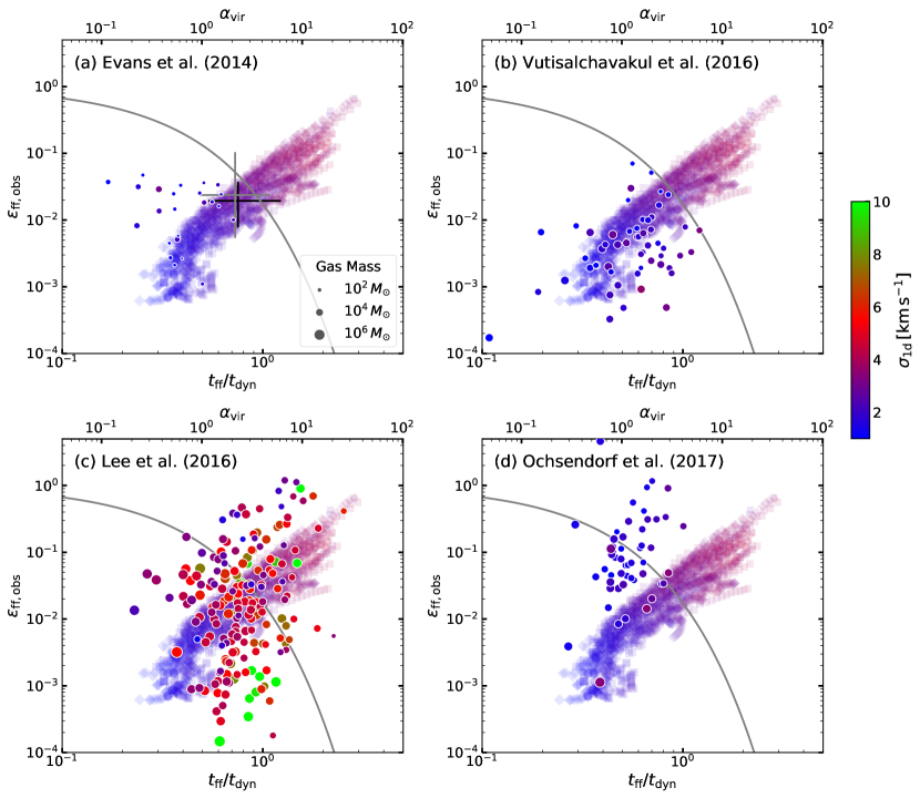
Figure 16: Relation between instantaneous $t_{\rm ff}/t_{\rm dyn}=(\pi^{2}/40)^{1/2}\alpha_{\rm vir}^{1/2}$ vs. $\varepsilon_{\rm ff,obs}$ in simulations (squares and diamonds; $\alpha$- and $\beta$-series models) and observations (circles). For simulations, we use the instantaneous mass, size, and velocity dispersion of the gas cloud and cluster’s bolometric UV luminosity. We show snapshots in the time interval $t_{*,0}<t<t_{*,90\%}$. The circles in different panels show data from different observational studies: (a) low-mass, nearby clouds compiled by Evans et al. (2014); (b) molecular clouds in the Galactic Plane with massive SFR $M_{*}>5\,M_{\odot}\,{\rm Myr}^{-1}$ (Vutisalchavakul et al., 2016). (c) GMCs with associated star-forming complexes in the Milky Way (Lee et al., 2016). (d) GMCs with associated star-forming complexes in the Large Magellanic Cloud (Ochsendorf et al., 2017). All data points are colored by one-dimensional velocity dispersion $\sigma_{\rm 1d}$ and their sizes denote gas mass. As in Figure 15, the solid gray line shows the fit to the $\alpha$-series models. In panel (a), the grey bars indicate the ranges of $\varepsilon_{\rm ff,0}$ and $t_{\rm ff,0}/t_{\rm dyn,0}$ in the $\alpha$-series plotted in Figure 15, while the black bars indicate the ranges of median values of $\varepsilon_{\rm ff,obs}$ and $t_{\rm ff}/t_{\rm dyn}$ for snapshots between $t_{*,0}$ and $t_{*,90\%}$.

Next, we compute the time-dependent, “observed” SFE per freefall time $\varepsilon_{\rm ff,obs}$ using mock observations of simulated clouds. For this exercise, we use the instantaneous cloud mass ($M_{\rm neu}$, assumed to be recoverable from molecular lines or dust emission), size ($R=2^{1/3}R_{50\%}$), and velocity dispersion ($\sigma_{\rm 1d}$) to compute the dynamical time $t_{\rm dyn}=R/\sigma_{\rm 1d}$ and the freefall time $t_{\rm ff}=\sqrt{3\pi/(32G\bar{\rho})}$, where $\bar{\rho}=3M_{\rm neu}/(4\pi R^{3})$. The instantaneous ratio $t_{\rm ff}/t_{\rm dyn}\propto\sigma_{\rm 1d}(R/M_{\rm neu})^{1/2}$.

Assuming that an observer is able to recover the cluster’s bolometric UV luminosity from massive star formation tracers such as H$\alpha$ and/or infrared fluxes, the instantaneous SFR is calculated as $\dot{M}_{*}=\Psi^{-1}L_{\rm UV}/t_{\rm UV}$, where $L_{\rm UV}=L_{\rm LyC}+L_{\rm FUV}$ is the bolometric UV luminosity. For the conversion factor between SFR and UV luminosity, we use the IMF-averaged light-to-mass ratio $\Psi=10^{3}\,L_{\odot}\,M_{\odot}^{-1}$ (see also Figure 17), and we adopt an effective lifetime of UV luminosity $t_{\rm UV}=6.7\,{\rm Myr}$ to be consistent with the relation $\dot{M}_{*}=1.5\times 10^{-4}\,M_{\odot}\,\,{\rm Myr}^{-1}(L_{\rm UV}/L_{\odot})$ widely adopted in observations (Kennicutt & Evans, 2012; Liu et al., 2020). This assumes a more exact age for the stellar system is not known, although with spectral fitting cluster ages can be obtained (e.g., Adamo et al., 2017). The observed SFE per freefall time is then $\varepsilon_{\rm ff,obs}=(t_{\rm ff}/t_{\rm UV})L_{\rm UV}/(\Psi M_{\rm neu})\propto M_{*}(R/M_{\rm neu})^{3/2}$.

Figure 16 plots as squares ($\alpha$-series) and diamonds ($\beta$-series) $\varepsilon_{\rm ff,obs}$ for all models as a function of $t_{\rm ff}/t_{\rm dyn}$. The top axis also shows instantaneous $\alpha_{\rm vir}=(40/\pi^{2})(t_{\rm ff}/t_{\rm dyn})^{2}$. We consider snapshots in the time range $t_{*,}<t<t_{*,90\%}$. The color of symbols indicates the 1D velocity dispersion. In contrast with $\varepsilon_{\rm ff,0}$ in Figure 15, all of our models start from the lower left with $\alpha_{\rm vir}\sim 0.5$–$1.5$ and $\varepsilon_{\rm ff,obs}\sim 10^{-3}$, and, as time progresses, they move upward slightly and then to the upper right. This trajectory reflects the evolution of cloud’s gas mass, size, and velocity dispersion, and the cluster’s mass and luminosity. The stellar mass $M_{*}$ and UV luminosity start very small and keep increasing during the main star formation phase (note that $t_{\rm SF}$ is comparable to or shorter than $t_{\rm UV}$, except for a small number of late snapshots in strongly magnetized clouds). Meanwhile, radiation feedback drives mass loss and radial expansion, leading to an increase in $R/M_{\rm neu}$, together with an increase in velocity dispersion $\sigma_{\rm 1d}$. As a result, evolution causes $\varepsilon_{\rm ff,obs}\propto M_{*}(R/M_{\rm neu})^{3/2}$ and $t_{\rm ff}/t_{\rm dyn}\propto\sigma_{\rm 1d}(R/M_{\rm neu})^{1/2}$ to increase in tandem. The distribution of $t_{\rm ff}/t_{\rm dyn}$ extends to larger values (by a factor of a few) than in Figure 15 due to cloud evolution. Even more extreme is the stretch in the distribution of $\varepsilon_{\rm ff,obs}$ by two orders of magnitude compared to $\varepsilon_{\rm ff,0}$ in Figure 15. We note, however, that in their later stages, the simulated systems have very low gas mass (leading to $\varepsilon_{\rm ff,obs}\gtrsim 0.1$ and $t_{\rm ff}/t_{\rm dyn}\gtrsim 1$). While we include the full evolution for completeness, clouds in these stages would not necessarily be included in observed samples of star-forming GMCs.

Although there is a large variation during the evolution, we calculate the “characteristic” values of $t_{\rm ff}/t_{\rm dyn}$ and $\varepsilon_{\rm ff,obs}$ as a median for snapshots equally spaced in time between $t_{*,0}$ and $t_{*,90\%}$. We find $0.54<{\rm med}(t_{\rm ff}/t_{\rm dyn})<1.08$ and $0.8\%<{\rm med}(\varepsilon_{\rm ff,obs})<3.7\%$ in the $\alpha$-series models, while $0.54<{\rm med}(t_{\rm ff}/t_{\rm dyn})<1.23$ and $0.8\%<{\rm med}(\varepsilon_{\rm ff,obs})<3.5\%$ in the $\beta$-series models. The black bars in Figure 16(a) indicate the ranges of the medians. These values are similar to the ranges of $t_{\rm ff,0}/t_{\rm dyn,0}$ and $\varepsilon_{\rm ff,0}$ shown in Figure 15, as indicated by gray bars in Figure 16(a).

The circles in each panel show estimates of $t_{\rm ff}/t_{\rm dyn}$ and $\varepsilon_{\rm ff}$ for observed star-forming clouds, colored by one-dimensional velocity dispersion. Panel (a) shows the low-mass, nearby cloud sample taken from Evans et al. (2014), in which the cloud mass and size are derived from extinction maps, velocity dispersion from molecular linewidth (mostly ${}^{13}{\rm CO}$), and SFRs from counting young stellar objects (YSOs). Panel (b) shows the sample of larger molecular clouds in the Galactic Plane with ongoing massive star formation, compiled by Vutisalchavakul et al. (2016) (their Fig. 6). In their study, the cloud properties are derived from ${}^{13}{\rm CO}$ observations and SFR is determined from mid-infrared (MIR) luminosity. Following Vutisalchavakul et al. (2016), we exclude clouds with $\dot{M}_{*}<5\,M_{\odot}\,{\rm yr}^{-1}$ as MIR emission may seriously underestimate the true SFR at low SFR (even for cases shown, the MIR-based SFR may be underestimated by a factor $2$–$3$). Panel (c) shows the Milky Way GMCs with associated star-forming complexes in Lee et al. (2016) (their Fig. 7). Their samples are built from the ${}^{12}{\rm CO}$ catalog of molecular clouds (Miville-Deschênes et al., 2017), cross-correlated with WMAP free-free sources. Panel (d) shows the star forming complexes in the Large Magellanic Cloud (Ochsendorf et al., 2017). The cloud properties are identified by ${}^{12}{\rm CO}$ and SFR from H$\alpha$ + $24\mu{\rm m}$. We note that they multiplied the H$\alpha$-based SFR by a factor of 2 to account for the fact that the diffuse H$\alpha$ emission (outside the star-forming regions) constitutes 50% of the total H$\alpha$ emission (Pellegrini et al., 2012).

The results for $\varepsilon_{\rm ff,obs}$ from the simulations are generally similar to the observations, especially for the Vutisalchavakul et al. (2016) sample. However, the observations show no significant correlation of SFE per freefall time with $t_{\rm ff}/t_{\rm dyn}$. This discrepancy is partly due to the fact that points from the simulations extend towards large $t_{\rm ff}/t_{\rm dyn}$ and $\varepsilon_{\rm ff,obs}$ for clouds in the dispersing stages, which would be unlikely be included in the observational samples. Furthermore, the (extended) theoretical fit of $\varepsilon_{\rm ff,0}$ vs. $t_{\rm ff,0}/t_{\rm dyn,0}$ to our $\alpha$-series (shown in grey) does not follow the same trend as the correlation of time-dependent “observables” from the simulations. We conclude that evolutionary effects (the correlated increase over time of stellar mass, cloud size, and velocity dispersion along with the decrease of gas mass), which tend to make $\varepsilon_{\rm ff,obs}$ increase with $t_{\rm ff}/t_{\rm dyn}$ in Figure 16, completely obscure the underlying decrease of $\varepsilon_{\rm ff,0}$ with $t_{\rm ff,0}/t_{\rm dyn,0}$ seen in Figure 15.

Also, while the observed SFE per freefall time is small on average, it exhibits large intrinsic scatter. As discussed by previous authors, the large scatter in $\varepsilon_{\rm ff,obs}$ may arise for a number of reasons. First, as in our mock observed clouds, sampling clouds at different evolutionary stages (low stellar mass and high gas mass at an early evolutionary stage and the opposite at a later stage), is an important source of scatter (see also Grudić et al., 2019). Second, if the SFR in a cloud accelerates with time it will tend to produce a large scatter in $\varepsilon_{\rm ff,obs}$ (e.g., Lee et al., 2016) (although in fact we do not find evidence for accelerating SFR in our simulations). Third, poor sampling of the IMF at the high-mass end can be a source of large scatter and bias in the light-to-mass ratio and hence the inferred SFR, especially for SFR tracers relying on ionizing radiation (e.g., da Silva et al., 2014; Geen et al., 2018). Fourth, some variations can be induced by the distribution of $\alpha_{\rm vir,0}$ and $\mu_{\Phi,0}$ of initial clouds (e.g., Federrath, 2013), which in reality would represent a varying dynamical environment where molecular clouds form. In addition, there is scatter introduced in the observational estimation of cloud mass and $t_{\rm ff}$, largely because the former usually depends on conversion from CO luminosity via $X_{\rm CO}$, which is known from both observations and modeling to have significant scatter (e.g., Pineda et al., 2008; Shetty et al., 2011a, b; Seifried et al., 2020; Gong et al., 2020). Adopting a constant value of $X_{\rm CO}$ at cloud scales adds to the error in the estimated gas mass, which enters as $\varepsilon_{\rm ff,obs}\propto X_{\rm CO}^{-3/2}$ and $t_{\rm ff}/t_{\rm dyn}\propto X_{\rm CO}^{-1/2}$.

Our analysis shows that evolutionary effects make it difficult to test certain predictions from star formation theory/simulations with observations of individual molecular clouds. Looking forward, however, large extragalactic surveys that sample varying large-scale ISM/environments as well as different stages of cloud evolution (e.g., EDGE, PHANGS: Bolatto et al., 2017; Sun et al., 2020b) may be useful for testing model predictions. In particular, the anti-correlation between $\alpha_{\rm vir,0}$ and $\varepsilon_{\rm ff,0}$ seen in our simulations (Figure 15) can be investigated by inter-comparing population-averaged cloud properties in different galactic environments; at a given galactocentric radius, $\alpha_{\rm vir,0}$ can be estimated from the cloud-scale $\alpha_{\rm vir}$ averaged over non-star-forming clouds, while $\varepsilon_{\rm ff,0}$ can be estimated by taking the cloud-scale $t_{\rm ff}$ averaged over the same clouds, multiplying by the annular SFR, and dividing by the total mass of (non-star-forming) molecular gas in the annulus. By averaging over azimuthal angle at a given radius, it can be ensured that all stages of (early) evolution are represented. For better leverage, comparisons based on widely ranging environments are likely to be most useful – e.g., atomic-dominated outer disks, molecule-dominated inner disks, and galactic centers (including starbursts). Galactic regions with high or low ratios of stellar-to-gas vertical gravity may also have systematically higher or lower mean values of $\alpha_{\rm vir}$.

A recent compilation study by Schruba et al. (2019) including both Milky Way and extragalactic (8 galaxies) samples of GMCs indeed found that molecular clouds in atomic-dominated, low-pressure environment follow the decreasing trend of $\varepsilon_{\rm ff}$ with $\alpha_{\rm vir}$, although this trend is lacking for clouds in molecule-dominated, high-pressure environments. Schruba et al. (2019) also emphasized that only by averaging cloud properties over the whole population can dependencies on environment become evident. Future studies utilizing homogeneous datasets will be desirable to draw more statistically significant conclusions.

6 Summary and Discussion

6.1 Summary

In this work, we have presented a suite of RMHD simulations modeling the evolution of a turbulent, magnetized GMC and its dispersal by UV radiation feedback from embedded star clusters. Our simulations model radiation from both internal cluster particles (using adaptive ray tracing) and external sources (using the six-ray approximation). The radiative transfer calculation is coupled with a simple photochemistry module that follows the non-equilibrium abundances of molecular, atomic, and ionized hydrogen as well as equilibrium abundances of C- and O-bearing species. Dynamical evolution is driven by the high thermal pressure of the ionized (photoevaporated) gas, and by the radiation pressure of both LyC and FUV on the gas/dust.

Our model clouds all have a common initial mass $M_{\rm 0}=10^{5}\,M_{\odot}$, radius $R_{\rm 0}=20\,{\rm pc}$, and freefall time $t_{\rm ff,0}=4.68\,{\rm Myr}$. They differ in the initial level of turbulence and in the initial uniform magnetic field that threads the clouds. In the $\alpha$-series models, we vary the initial kinetic virial parameter $\alpha_{\rm vir,0}$ between 1 and 5 and adopt a fixed initial mass-to-magnetic flux ratio $\mu_{\Phi,0}=2$ (relative to the critical mass-to-flux). In the $\beta$-series models, we adopt a fixed $\alpha_{\rm vir,0}=2$, while varying $\mu_{\Phi,0}$ between $0.5$ and $8$; we also consider the unmagnetized case ($\mu_{\Phi,0}=\infty$). For each cloud model with a given ($\alpha_{\rm vir,0}$, $\mu_{\Phi,0}$), we run five simulations with different turbulence realizations. Our fiducial model has $(\alpha_{\rm vir,0},\mu_{\Phi,0})=(2,2)$, corresponding to an initial 1D velocity dispersion of $2.9\,{\rm km}\,{\rm s}^{-1}$ and magnetic field strength of $13.5\mu{\rm G}$.

The following summarizes key results from our work:

1. Overall Evolution. Clouds in our simulations undergo the following evolutionary stages: (1) development of filamentary structures, (2) formation of sink particles and compact H II regions within filaments, (3) breakout and merging of H II regions that photoevaporate and dynamically eject the cold neutral gas, leading ultimately to quenching of star formation. Compared to the fiducial model, stronger turbulence in initially unbound ($\alpha_{\rm vir,0}>2$) clouds makes them expand in size and lose a larger fraction of neutral gas as outflows (Figure 18 and Figure 5(e)). In strongly magnetized clouds ($\mu_{\Phi,0}\leq 1$), filaments are aligned predominantly perpendicular to the direction of large-scale magnetic fields (Figure 19) and the motion of (both neutral and ionized) gas is highly anisotropic (Figures 4 and 5(j)). Models with different turbulence realizatons show that the initial large-scale velocity field and its relative orientation to the magnetic field affect the details of structure formation and ensuing cluster formation, giving rise to moderate variations in simulation outcomes (Figures 8–12 and Table 2).

2. Star Formation Rate and Efficiency. For all models, UV radiation feedback is very effective in dispersing gas and keeping the final cloud-scale SFE low. Both the final SFE and the SFR are reduced in models with strong turbulence and magnetic fields. The median value of the final SFE ($\varepsilon_{*}$) ranges between $2.1\%$ and $9.5\%$ in the $\alpha$-series and between $2.4\%$ and $8.2\%$ in the $\beta$-series models, systematically increasing with decreasing $\alpha_{\rm vir,0}$ and increasing $\mu_{\Phi,0}$. Different realizations of turbulence lead to an additional $\sim 2$–$5\%$ variation in the final SFE. The SFE at the nominal time of the first supernovae ($\varepsilon_{*,{\rm 3Myr}}$) ranges between $0.5\%$ and $7\%$ and is about $50^{+20}_{-20}\%$ of the final SFE (Figure 9). The time-averaged SFR $\langle\dot{M}_{*}\rangle$ is systematically lower at higher $\alpha_{\rm vir,0}$ and lower $\mu_{\Phi,0}$ (Figure 8). The median value of the gas depletion timescale $t_{\rm dep,0}=M_{\rm 0}/\langle\dot{M}_{*}\rangle$ ranges between $58$–$255\,{\rm Myr}$ in the $\alpha$-series models and $61$–$464\,{\rm Myr}$ in the $\beta$-series models.

3. Mass Loss Efficiency. In most of our simulated clouds, the majority of cloud mass is lost via photoevaporation followed by dynamical ejection ($\varepsilon_{\rm ion}\sim 0.6$–$0.8$; Figure 10). Initially unbound clouds have a higher fraction of gas ejected as neutrals due to expansion driven by initial turbulence. In strongly magnetized clouds, most of the gas is ejected in the atomic phase due to the low ionizing photon rate and magnetic confinement, which limits escape routes of the gas.

4. Evolutionary Timescales. The median value of the time at which the first star formation occurs ($t_{*,0}$) is $3.5$–$4.3\,{\rm Myr}$ in the $\alpha$-series models and $2.1$–$8.6\,{\rm Myr}$ in the $\beta$-series models. Except for the magnetically subcritical clouds (A2B05), clouds in our simulations form stars on timescales of $t_{\rm SF}\sim 5$–$7\,{\rm Myr}$ (or $1$–$1.5$ freefall times) and are destroyed within $t_{\rm dest,H_{2}}\sim 6$–$9\,{\rm Myr}$ (or $1.3$–$2.0$ freefall times) after the onset of radiation feedback (Figure 11). Magnetically subcritical clouds have longer evolutionary timescales because of the low SFR and inefficient mass loss processes. Since SFRs are approximately constant, the average observed age of the stellar clusters in an actively star-forming cloud would be approximately $t_{\rm SF}/3\sim 2\,{\rm Myr}$.

5. Escape of Radiation. The cumulative median escape fraction of LyC (FUV) radiation ranges between $21$–$34\%$ ($53$–$69\%$) in the $\alpha$-series models and between $13$–$33\%$ ($57$–$64\%$) in the $\beta$-series. The escape fraction is low in magnetically subcritical clouds because of reduced gas compressibility, which results in less porous structure. Different turbulent realizations yield greater variation in $f_{\rm esc,Lyc}$ than in $f_{\rm esc,FUV}$.

6. Virial Ratios. We study the evolution of the virial ratio $\tilde{\alpha}_{\rm vir,tot}$ that accounts for kinetic, thermal, and magnetic energies of the neutral cloud, and compare it with the traditional kinetic virial parameter $\alpha_{\rm vir}=5R\sigma_{\rm 1d}^{2}/(GM_{\rm neu})$ based on the cloud mass, size, and velocity dispersion (Figures 5 and 13). The virial ratio decreases due to decaying turbulence at early times, but it increases to large values ($\tilde{\alpha}_{\rm vir,tot}>10$) at late times as feedback disperses the cloud. In spite of the widely ranging initial conditions of the models, at the time of the first star formation the median value of $\tilde{\alpha}_{\rm vir,tot}$ falls in a fairly narrow range $0.9$–$2.2$ (except for the magnetically subcritical clouds, for which the median value is $6.7$). In strongly magnetized clouds, the kinetic energy may be significantly underestimated or overestimated depending on the relative orientation between the observer’s line of sight and the direction of magnetic field. Averaging over directions (as would be possible with an ensemble average in observations), the traditional virial parameter generally agrees with $\tilde{\alpha}_{\rm vir,tot}$ within a factor of two. However, gravitational boundedness is systematically overestimated when $\alpha_{\rm vir}$ is used, due to the neglect of magnetic energy. We also discuss approximate relations (Equations (23)–(25)) that would be satisfied by an ensemble of molecular clouds in statistical equilibrium, and how the importance of magnetic support can be indirectly inferred from observations.

7. SFE per freefall time. The median value of the SFE per freefall time based on the time-averaged SFR and the initial cloud mass and size ($\varepsilon_{\rm ff,0}=t_{\rm ff,0}\langle\dot{M}_{*}\rangle/M_{\rm 0}$) ranges between $1.8$–$8.0\%$ in the $\alpha$-series and $1.0$–$7.7\%$ in the $\beta$-series, higher at lower $\alpha_{\rm vir,0}$ (weak turbulence) and higher $\mu_{\Phi,0}$ (weak mean magnetic fields) (bottom row of Figure 11 and Figure 15). However, the dependence of $\varepsilon_{\rm ff,0}$ on $\mu_{\Phi,0}$ is very slight in the magnetically supercritical regime. The functional form $\varepsilon_{\rm ff,0}=\exp(-Ct_{\rm ff,0}/t_{\rm dyn,0})$ (similar to Padoan et al., 2012, from driven-turbulence simulations) well describes the results of the $\alpha$-series models, with the best-fit parameter $C=4.06$. The decreasing trend of $\varepsilon_{\rm ff,0}$ with $t_{\rm ff,0}/t_{\rm dyn,0}\propto\alpha_{\rm vir,0}^{1/2}$ is also in qualitative agreement with some theoretical models for SFR based on a density threshold and log-normal density PDF, although others follow different trends (e.g., Krumholz & McKee, 2005; Hennebelle & Chabrier, 2011; Federrath & Klessen, 2012). Nevertheless, observational validation is challenging because the relation between instantaneous measurements $\varepsilon_{\rm ff,obs}(t)$ and $\alpha_{\rm vir}(t)$ (as would be available in observations) shows a quite different (almost orthogonal) trend from both numerical measurements and theoretical models of $\varepsilon_{\rm ff,0}$. The increase in $\varepsilon_{\rm ff,obs}\propto M_{*}(R/M_{\rm neu})^{3/2}$ with instantaneous $t_{\rm ff}/t_{\rm dyn}\propto\sigma_{\rm 1d}(R/M_{\rm neu})^{1/2}$ owes to rapidly evolving cloud and cluster properties (physical expansion of the cloud combined with conversion of neutral gas to stars and ionized gas) which affect both quantities in the same way. This “evolutionary masking” explains why observations of star-forming clouds fail to reproduce the decline of $\varepsilon_{\rm ff,0}$ with $\alpha_{\rm vir,0}$ predicted by the theory (Figure 16).

6.2 Discussion

Our conclusions regarding the rapid and efficient dispersal of GMCs by ionizing and non-ionizing UV are in agreement with our previous findings in Kim et al. (2018). There, we focused on how evolution and final outcomes depend on the cloud surface density (for a range $\Sigma_{\rm 0}\approx 10$–$10^{3}\,M_{\odot}\,{\rm pc^{-2}}$), and found that in all cases star formation is quenched and clouds are dispersed within a few freefall times or several Myr after star formation commences. Our new simulations, with more realistic physics (addition of realistic thermochemistry, magnetic fields, and time-dependent luminosity) confirm this evolutionary scenario. The short timescales we find are also consistent with recent empirical constraints on rapid cloud dispersal after the onset of star formation (e.g., Kruijssen et al., 2019; Chevance et al., 2020b, c; Kim et al., 2020b).

Our findings of decreasing SFR and net SFE with increasing $\alpha_{\rm vir,0}$ are consistent with findings from previous hydrodynamical simulations of global clouds (e.g., Raskutti et al., 2016; Bertram et al., 2015; Howard et al., 2016; Dale, 2017; Kim et al., 2018), as well as hydrodynamic and MHD simulations with driven turbulence in a periodic box (Padoan et al., 2012). General theoretical expectations as well as some numerical simulations (e.g., Federrath, 2015) suggest lower SFR and SFE in magnetized compared to unmagnetized clouds, but we are not aware of a previous systematic numerical study of the dependence on global mass-to-magnetic flux ratio with massive star feedback.

While traditionally it was usually assumed that the virial parameter is close to unity for GMCs (Solomon et al., 1987), recent extragalactic surveys of molecular gas on scales $\sim 50$–$100\,{\rm pc}$ have instead found that the typical (kinetic) virial parameter may be closer to 4 than 1 (Sun et al., 2020b). Measurements of pressure also show that only half can be accounted for by the self-gravity of the cloud (Sun et al., 2020a), which again suggests $\alpha_{\rm vir}>2$. Thus, our $\alpha_{\rm vir}\sim 4-5$ models are likely the most realistic, and it is these that have the lowest $\varepsilon_{\rm ff,0}\sim 2-3\%$. While the estimate of the mean $\varepsilon_{\rm ff}$ from the large extragalactic PHANGS survey is closer to $\sim 1\%$ (Utomo et al., 2018), it must be borne in mind that whole-galaxy averages include diffuse and quiescent molecular gas in clouds prior to the onset of star formation. For our simulations, the quiescent period in fact has comparable duration to the active star-forming epoch; averaging over both the non-star-forming and star-forming epochs would reduce the mean efficiency per unit time. The range of $\varepsilon_{*}$ in our simulations is in good agreement with estimates of the integrated cloud-scale SFE of $4$–$10\%$ obtained from the statistical analysis of ${\rm CO}$ and ${\rm H}\alpha$ emission in nearby star-forming galaxies (Chevance et al., 2020b).

As remarked in Section 3.2.2, the subcritical clouds ($\mu_{\Phi,0}=0.5$) have evolution very different from other models in several respects. These include an extremely long time until the first star formation followed by very slow star formation and dispersal (the lifetime can exceed $30\,{\rm Myr}$ for some seeds, and the final SFE $~{}\sim 2$–$3\%$), columnar outflow configuration, very low fraction of gas that is ionized, and extremely low escape fraction of LyC radiation, $f_{\rm esc,LyC}\sim 8-13\%$. The columnar outflow configuration of the subcritical models is not seen in observed GMCs, although recent evidence suggests that the dynamics of bipolar (or hourglass-shaped) H II regions on smaller scales is controlled by magnetic fields (e.g., Eswaraiah et al., 2017). In addition, the low $f_{\rm esc,LyC}$ from magnetically subcritical clouds appears insufficient to explain emission from diffuse ionized gas, which requires low-density channels in the large-scale ISM and also sufficient photons escaping from active star-forming clouds (see Kim et al., 2019b; Kado-Fong et al., 2020, and references therein). Another feature of the subcritical models is that the cloud typically consists of massive filaments aligned preferentially perpendicular to the mean magnetic field (e.g., top row of Figure 19). This feature, while unlike observations of GMCs, is reminiscent of the perpendicular alignment between magnetic fields and high-column structures in several nearby lower-mass ($M\lesssim 10^{4}\,M_{\odot}$) dark molecular clouds (e.g., Soler et al., 2016). This raises the interesting possibility that observed dark clouds, which have low overall SFE and lack of high-mass stars (e.g., Evans et al., 2009), may be magnetically subcritical. With slow star formation and low total mass, they may typically be destroyed (by external supernova shocks) before they ever form high-mass stars.

We note that our reported values for $\varepsilon_{*}$ are higher than the predictions for the SFE ($\sim 1\%$) based on idealized spherical shell expansion (Kim et al., 2016; Rahner et al., 2019; Inoguchi et al., 2020) even though the physical processes (ionized gas pressure and radiation pressure) in those spherical models are included in our simulations. As explained previously in Kim et al. (2018), several factors contribute to higher SFEs in realistic (non-spherical) models. One factor is the filamentary nature of the gas distribution, which allows a significant fraction of radiation to escape without contributing direct radiation pressure or photoevaporating neutral gas and helping to maintain the thermal pressure in ionized gas. Also, given the turbulent nature of clouds and multiple sources, thermal and radiation pressure forces may partially cancel, unlike the situation for a spherical cloud with a central source. In clouds with realistic structure, forces derived from feedback are reduced by an order of magnitude compared to simple spherical estimates (e.g., Figure 13 of Kim et al. 2018).

While idealized analytic studies are valuable for identifying key physical effects and predicting trends in parameter dependence, numerical simulations with realistic geometry and accurate physical treatments are required in order to obtain quantitative predictions for SFRs and SFEs. Indeed, idealized spherical evolution driven by ionized gas pressure and radiation pressure does not even include the photoevaporation mechanism, which we find (as in Kim et al. 2018) is the main means for dispersing the cloud. Although not always taken under consideration in simple treatments of cloud destruction (e.g., Chevance et al., 2020c), we note more generally that photoevaporation and self-acceleration of ionized gas is a distinct mechanism from acceleration of neutral gas by the pressure of confined photoionized gas, and results in a much larger fraction of gas becoming ionized and ejected.

Ejected ions can explain the low-density ionized gas (“halo”) surrounding individual H II regions (e.g., Anderson et al., 2015; Luisi et al., 2020), but this process is not likely to be the immediate source of diffuse ionized gas in the larger-scale ISM. The reason is that both the lifetime of ionizing sources in a given cloud and the gas recombination time scale are short compared to the timescale which ejected ionized gas would require to reach and fill the distant diffuse ISM. The ejected photoionized gas would become neutral on a recombination timescale ($t_{\rm rec}\sim(n_{\rm H}/0.1\,{\rm cm}^{-3})^{-1}\,{\rm Myr}$) after the death of ionizing stars, or if the path to radiation sources becomes obstructed.

The present simulations have made a significant advance over previous work in terms of physical realism. However, there is still more to be done. One limitation of the present simulations is the isolated nature of clouds. The isolation of clouds means that they are not affected by events in the surrounding ISM, which in reality may be important in high density environments such as spiral arms where GMCs are near neighbors. These events include supernovae from neighboring, more mature star-forming regions, which may destroy a cloud before star formation reaches the limit imposed by its own internal feedback.

A second limitation is the idealized initial condition with uniform density and magnetic field. Our model clouds become highly filamentary before star formation commences, so we do not consider the uniform spherical initial condition in itself a serious issue. However, our model clouds are at much higher density than the mean ISM, and it is clearly desirable to follow the ISM condensation processes that form GMCs at high resolution with comprehensive physics, not least because this removes the need to artifically set an initial virial parameter and mass-to-flux ratio. Zoom-in simulations (e.g., Seifried et al., 2017; Haid et al., 2019; Seifried et al., 2020) offer a route to a more complete and holistic numerical study of molecular cloud lifecycle, from formation to destruction.

A third limitation is related to our treatment of star formation. In our simulations, we use sink particles, which are relatively massive, to represent regions of the cloud that have collapsed gravitationally. Because our approach does not resolve individual stars, we adopt the same time-dependent light-to-mass ratio for all particles, which assumes a fully-sampled IMF. While our clouds are massive enough that a fully-sampled IMF is reasonable over the lifetime of the cloud, stochastic IMF sampling is not properly represented during the earlier formation stages. Sampling from the IMF would lead to additional statistical variations in the lifetime SFE (Grudić & Hopkins, 2019) on top of those we have found from turbulence sampling, since clouds that happen to form more high-mass stars early would be able to quench star formation more rapidly, and vice versa for those with late formation of massive stars. Simple methods for IMF sampling have been developed to address this (Sormani et al., 2017), but just as for turbulence sampling, IMF sampling greatly increases the total computational expense because multiple runs are needed.

Beyond addressing the above issues, another important goal for future work is to include additional forms of feedback, rather than only radiation. In particular, stellar winds may be important at early stages after star clusters form (especially in very dense clouds; e.g., Lancaster et al. 2020 submitted), while supernovae may be important at late stages (in low density clouds with long lifetimes; e.g., Fall et al. 2010). However, the reduction of the Courant–Friedrichs–Lewy timestep necessary to follow hot gas implies considerably higher computational expense. This underscores the imperative for numerical algorithms that both represent the underlying equations accurately, and are performance-optimized for modern computational platforms.

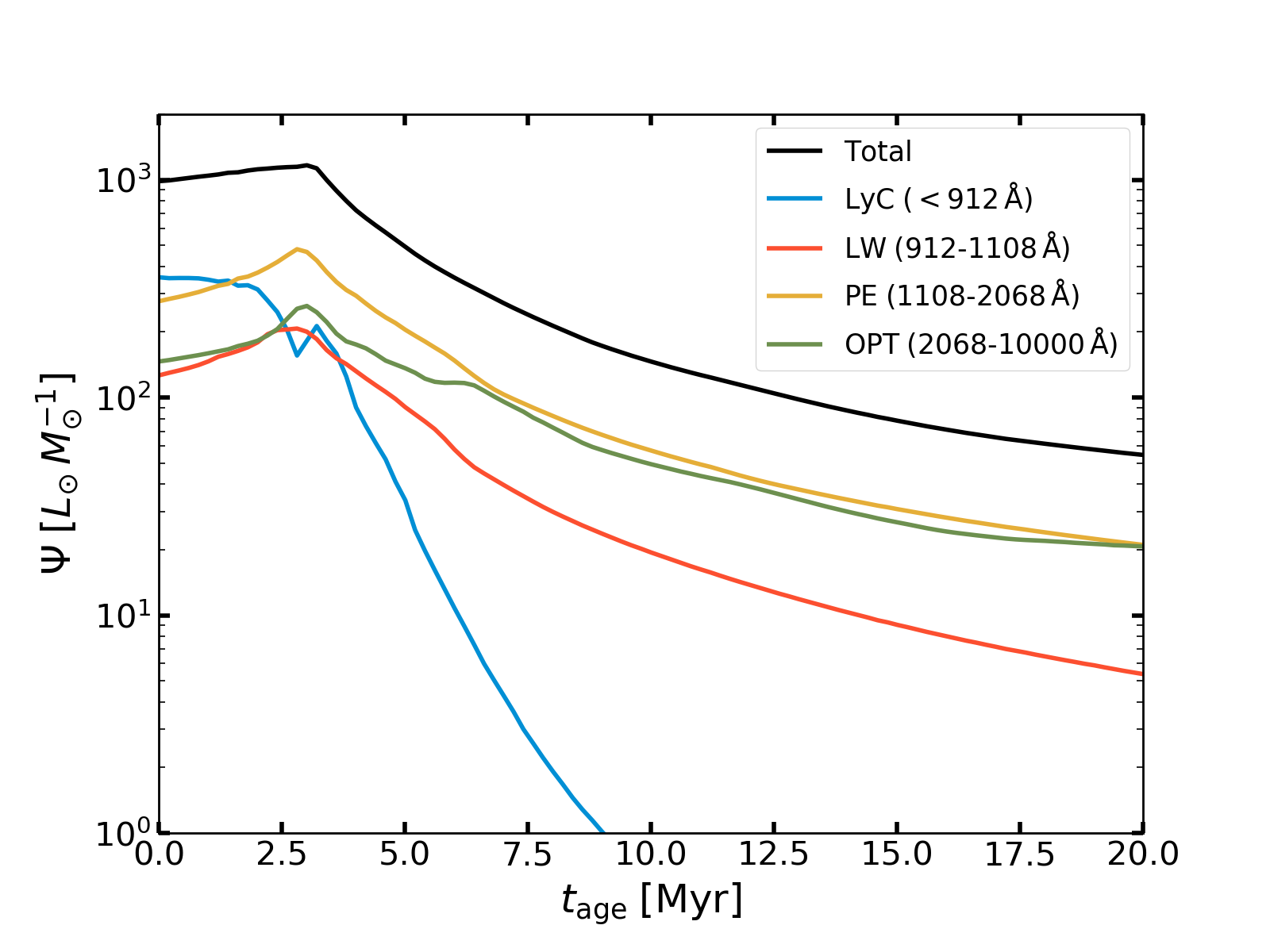
Figure 17: Luminosity per unit mass $\Psi$ as a function of the age of a star cluster sampling the Kroupa IMF. Different lines show $\Psi$ in different frequency bins: H-ionizing (LyC), photoelectric and ${\rm H_{2}}$-dissociating (LW), photoelectric (PE), and optical (OPT) wavelength range.

Appendix A Radiative Output from Star Clusters

We use the Starburst99 stellar population synthesis code (Leitherer et al., 2014) to calculate the radiative output per unit mass $\Psi=L_{*}/M_{*}$ from a coeval stellar population fully sampling the Kroupa IMF in the mass range of $0.1$–$100\,M_{\odot}$. We adopt the Geneva evolutionary tracks for non-rotating, solar metallicity stars and Pauldrach + Hillier stellar atmosphere models. Figure 17 shows the luminosity per unit mass as a function of age in different frequency bins. The conversion factors for ionizing (LyC) and non-ionizing (LW+PE) UV photons drop to 50% of the initial value after $3\,{\rm Myr}$ and $6\,{\rm Myr}$, respectively. The ratios $\Psi_{\rm LW}/\Psi_{\rm PE}$ and $\Psi_{\rm OPT}/\Psi_{\rm PE}$ range between $0.25$–$0.5$ and $0.5$–$1$ for $t_{\rm age}<20\,{\rm Myr}$.

Appendix B Snapshots of Representative Models

To provide a sense of the differences in evolution for different models, here we present comparison snapshots at times $t_{*,0}-0.2\,{\rm Myr}$, $t_{*,0}+2\,{\rm Myr}$, $t_{*,0}+5\,{\rm Myr}$, $t_{*,0}+8\,{\rm Myr}$, where $t_{*,0}$ is the time of first star formation. We show projections of gas surface density along the $y$ axis, so that individual panels have $x$ horizontal and $z$ vertical, with the initial magnetic field oriented along the $z$-direction.

Figure 18 compares members of the $\alpha$-series with different initial kinetic energy (increasing top to bottom) but identical initial relative amplitudes of all the different turbulent Fourier modes (seed$=4$) and initial mass-to-magnetic flux ratio $\mu_{\Phi,0}=2$. The second row shows the fiducial model. Members of the series with higher initial $\alpha_{\rm vir,0}$ disperse more rapidly and have a lower SFE.

Figure 19 compares members of the $\beta$-series with different initial magnetic energy (decreasing top to bottom) and an identical initial turbulence realization ($\alpha_{\rm vir,0}=2$, seed$=4$). The third row shows the fiducial model. Dense filamentary structures tend to be aligned perpendicular to the direction of the background magnetic field in strongly-magnetized models, and outflows driven by radiation are primarily parallel to the magnetic field. Weakly magnetized models are overall more isotropic in their evolution, evolve more rapidly, and have higher SFE.

Figure 20 compares different simulations with different initial turbulence seeds (i.e., different initial Fourier amplitudes of the turbulence) and the same value of $\alpha_{\rm vir,0}=2$, $\mu_{\Phi,0}=2$. Differences in the detailed turbulence realization can produce quite different morphological evolution, and there can also be significant differences in the SFE (see Figure 9) and other quantitative outcomes.

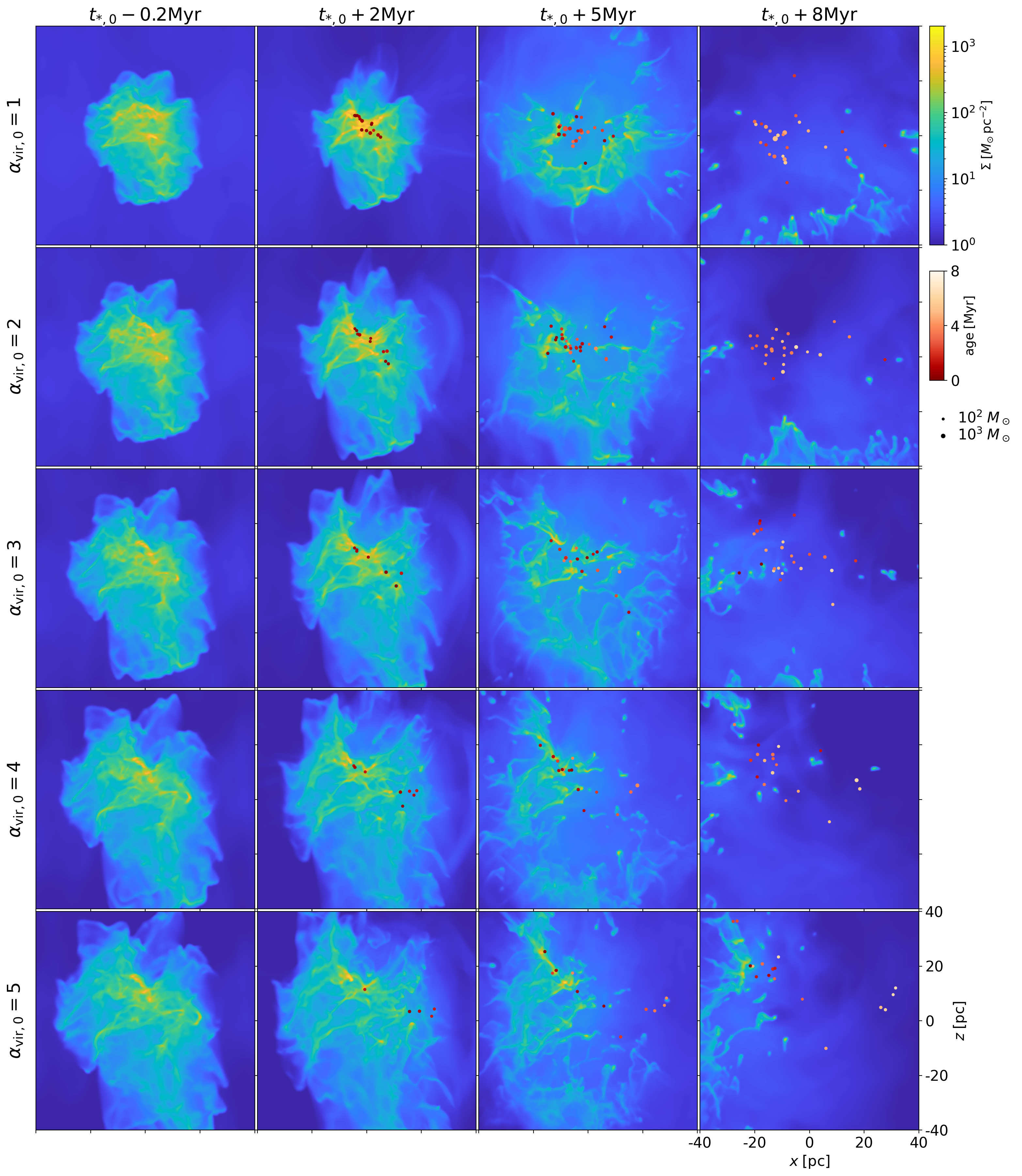
Figure 18: Snapshots of gas surface density projected along the $y$-axis from the $\alpha$-series models with ${\tt seed=4}$ From top to bottom, the initial virial parameter $\alpha_{\rm vir,0}$ increases from $1$ to $5$. The projected positions of star particles are indicated by circles. The size and color of circles indicate mass and age, respectively.

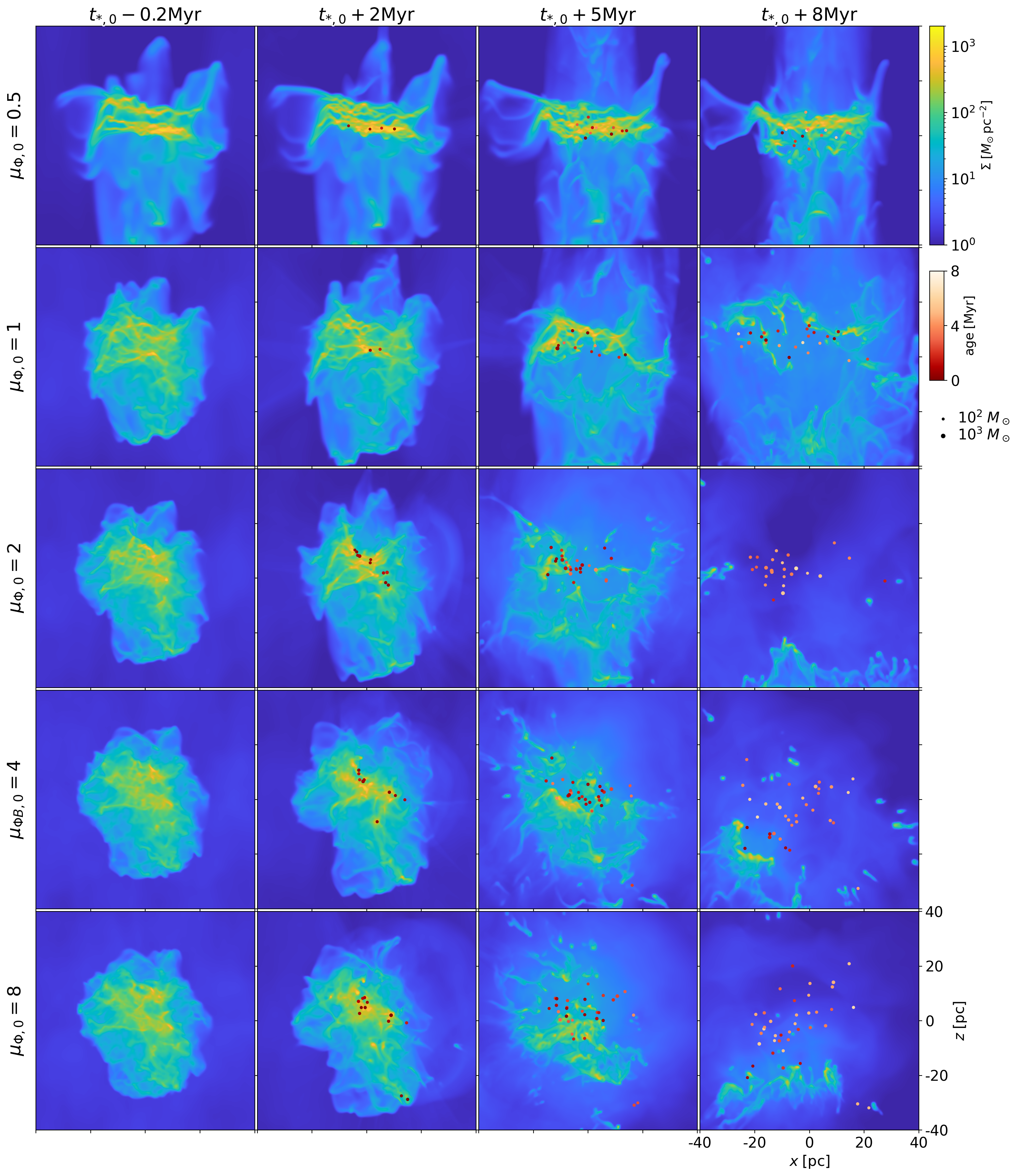
Figure 19: Same as Figure 18 but for the $\beta$-series modes with ${\tt seed=4}$, which have identical initial turbulent velocity field but varying initial magnetic field strength, decreasing from top to bottom. The corresponding initial mass-to-magnetic flux ratio $\mu_{\Phi,0}$ varies from $0.5$ to $8$.

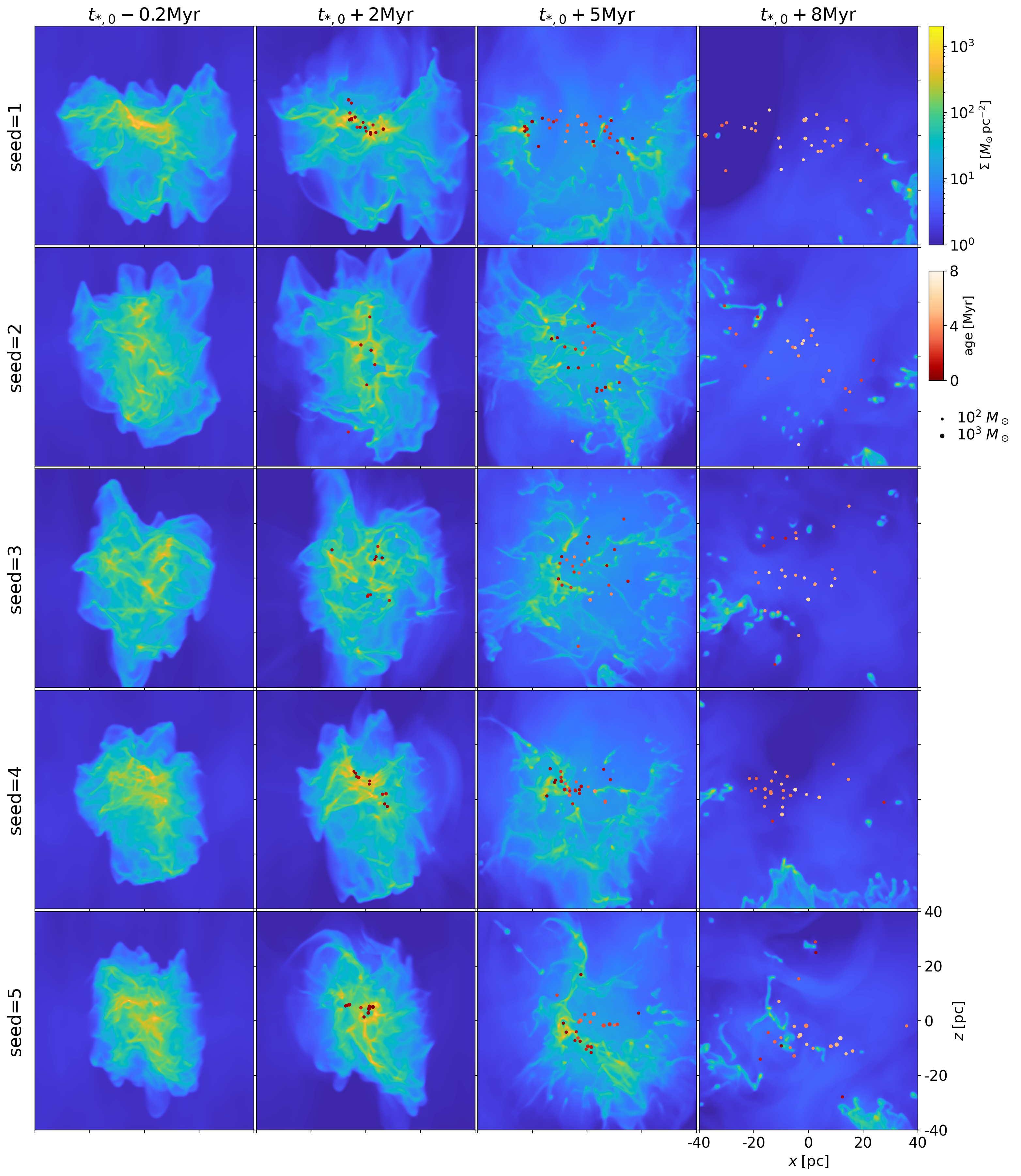
Figure 20: Same as Figure 18 but for the fiducial model ${\tt A2B2}$ with different random seeds for the initial turbulent velocity field.

References

- Adamo et al. (2017) Adamo, A., Ryon, J. E., Messa, M., et al. 2017, ApJ, 841, 131
- Adamo et al. (2020) Adamo, A., Zeidler, P., Kruijssen, J. M. D., et al. 2020, Space Sci. Rev., 216, 69
- Akimkin et al. (2015) Akimkin, V. V., Kirsanova, M. S., Pavlyuchenkov, Y. N., & Wiebe, D. S. 2015, MNRAS, 449, 440
- Akimkin et al. (2017) —. 2017, MNRAS, 469, 630
- Ali et al. (2018) Ali, A., Harries, T. J., & Douglas, T. A. 2018, MNRAS, 477, 5422
- Anderson et al. (2015) Anderson, L. D., Deharveng, L., Zavagno, A., et al. 2015, ApJ, 800, 101
- Arthur et al. (2011) Arthur, S. J., Henney, W. J., Mellema, G., de Colle, F., & Vázquez-Semadeni, E. 2011, MNRAS, 414, 1747
- Astropy Collaboration et al. (2013) Astropy Collaboration, Robitaille, T. P., Tollerud, E. J., et al. 2013, A&A, 558, A33
- Astropy Collaboration et al. (2018) Astropy Collaboration, Price-Whelan, A. M., Sipőcz, B. M., et al. 2018, AJ, 156, 123
- Ayachit (2015) Ayachit, U. 2015, The ParaView Guide: A Parallel Visualization Application (Clifton Park, NY, USA: Kitware, Inc.)
- Ballesteros-Paredes (2006) Ballesteros-Paredes, J. 2006, MNRAS, 372, 443
- Ballesteros-Paredes et al. (2009) Ballesteros-Paredes, J., Gómez, G. C., Pichardo, B., & Vázquez-Semadeni, E. 2009, MNRAS, 393, 1563
- Ballesteros-Paredes et al. (1999) Ballesteros-Paredes, J., Vázquez-Semadeni, E., & Scalo, J. 1999, ApJ, 515, 286
- Barnes et al. (2017) Barnes, A. T., Longmore, S. N., Battersby, C., et al. 2017, MNRAS, 469, 2263
- Bertoldi & McKee (1992) Bertoldi, F., & McKee, C. F. 1992, ApJ, 395, 140
- Bertram et al. (2015) Bertram, E., Glover, S. C. O., Clark, P. C., & Klessen, R. S. 2015, MNRAS, 451, 3679
- Binder & Povich (2018) Binder, B. A., & Povich, M. S. 2018, ApJ, 864, 136
- Bolatto et al. (2008) Bolatto, A. D., Leroy, A. K., Rosolowsky, E., Walter, F., & Blitz, L. 2008, ApJ, 686, 948
- Bolatto et al. (2017) Bolatto, A. D., Wong, T., Utomo, D., et al. 2017, ApJ, 846, 159
- Chastenet et al. (2019) Chastenet, J., Sandstrom, K., Chiang, I. D., et al. 2019, ApJ, 876, 62
- Chen et al. (2020) Chen, Y., Li, H., & Vogelsberger, M. 2020, arXiv e-prints, arXiv:2006.00004
- Chevance et al. (2020a) Chevance, M., Kruijssen, J. M. D., Vazquez-Semadeni, E., et al. 2020a, Space Sci. Rev., 216, 50
- Chevance et al. (2020b) Chevance, M., Kruijssen, J. M. D., Hygate, A. P. S., et al. 2020b, MNRAS, 493, 2872
- Chevance et al. (2020c) Chevance, M., Kruijssen, J. M. D., Krumholz, M. R., et al. 2020c, arXiv e-prints, arXiv:2010.13788
- Crutcher (1999) Crutcher, R. M. 1999, ApJ, 520, 706
- Crutcher (2012) —. 2012, ARA&A, 50, 29
- Crutcher et al. (2010) Crutcher, R. M., Wandelt, B., Heiles, C., Falgarone, E., & Troland, T. H. 2010, ApJ, 725, 466
- Cunningham et al. (2018) Cunningham, A. J., Krumholz, M. R., McKee, C. F., & Klein, R. I. 2018, MNRAS, 476, 771
- da Silva et al. (2014) da Silva, R. L., Fumagalli, M., & Krumholz, M. R. 2014, MNRAS, 444, 3275
- Dale (2015) Dale, J. E. 2015, New A Rev., 68, 1
- Dale (2017) —. 2017, MNRAS, 467, 1067
- Dale et al. (2012) Dale, J. E., Ercolano, B., & Bonnell, I. A. 2012, MNRAS, 424, 377
- Deharveng et al. (2010) Deharveng, L., Schuller, F., Anderson, L. D., et al. 2010, A&A, 523, A6
- Deharveng et al. (2015) Deharveng, L., Zavagno, A., Samal, M. R., et al. 2015, A&A, 582, A1
- Dib et al. (2007) Dib, S., Kim, J., Vázquez-Semadeni, E., Burkert, A., & Shadmehri, M. 2007, ApJ, 661, 262
- Draine (1978) Draine, B. T. 1978, ApJS, 36, 595
- Draine (2011a) —. 2011a, ApJ, 732, 100
- Draine (2011b) —. 2011b, Physics of the Interstellar and Intergalactic Medium (Princeton University Press)
- Draine & Bertoldi (1996) Draine, B. T., & Bertoldi, F. 1996, ApJ, 468, 269
- Eswaraiah et al. (2017) Eswaraiah, C., Lai, S.-P., Chen, W.-P., et al. 2017, ApJ, 850, 195
- Evans (1991) Evans, Neal J., I. 1991, in Astronomical Society of the Pacific Conference Series, Vol. 20, Frontiers of Stellar Evolution, ed. D. L. Lambert, 45
- Evans et al. (2014) Evans, Neal J., I., Heiderman, A., & Vutisalchavakul, N. 2014, ApJ, 782, 114
- Evans et al. (2009) Evans, Neal J., I., Dunham, M. M., Jørgensen, J. K., et al. 2009, ApJS, 181, 321
- Fall et al. (2010) Fall, S. M., Krumholz, M. R., & Matzner, C. D. 2010, ApJ, 710, L142
- Federrath (2013) Federrath, C. 2013, MNRAS, 436, 3167
- Federrath (2015) —. 2015, MNRAS, 450, 4035
- Federrath & Klessen (2012) Federrath, C., & Klessen, R. S. 2012, ApJ, 761, 156
- Franco et al. (1994) Franco, J., Shore, S. N., & Tenorio-Tagle, G. 1994, ApJ, 436, 795
- Fukui & Kawamura (2010) Fukui, Y., & Kawamura, A. 2010, ARA&A, 48, 547
- Fukushima et al. (2020) Fukushima, H., Yajima, H., Sugimura, K., et al. 2020, MNRAS, 497, 3830
- Gardiner & Stone (2008) Gardiner, T. A., & Stone, J. M. 2008, Journal of Computational Physics, 227, 4123
- Geen et al. (2016) Geen, S., Hennebelle, P., Tremblin, P., & Rosdahl, J. 2016, MNRAS, 463, 3129
- Geen et al. (2017) Geen, S., Soler, J. D., & Hennebelle, P. 2017, MNRAS, 471, 4844
- Geen et al. (2018) Geen, S., Watson, S. K., Rosdahl, J., et al. 2018, MNRAS, 481, 2548
- Glatzle et al. (2019) Glatzle, M., Ciardi, B., & Graziani, L. 2019, MNRAS, 482, 321
- Glover & Mac Low (2007) Glover, S. C. O., & Mac Low, M.-M. 2007, ApJS, 169, 239
- Gong & Ostriker (2013) Gong, H., & Ostriker, E. C. 2013, ApJS, 204, 8
- Gong et al. (2018) Gong, M., Ostriker, E. C., & Kim, C.-G. 2018, ApJ, 858, 16
- Gong et al. (2020) Gong, M., Ostriker, E. C., Kim, C.-G., & Kim, J.-G. 2020, arXiv e-prints, arXiv:2009.14631
- Gong et al. (2017) Gong, M., Ostriker, E. C., & Wolfire, M. G. 2017, ApJ, 843, 38
- González-Samaniego & Vazquez-Semadeni (2020) González-Samaniego, A., & Vazquez-Semadeni, E. 2020, MNRAS, 499, 668
- Górski et al. (2005) Górski, K. M., Hivon, E., Banday, A. J., et al. 2005, ApJ, 622, 759
- Grasha et al. (2018) Grasha, K., Calzetti, D., Bittle, L., et al. 2018, MNRAS, 481, 1016
- Grasha et al. (2019) Grasha, K., Calzetti, D., Adamo, A., et al. 2019, MNRAS, 483, 4707
- Gritschneder et al. (2010) Gritschneder, M., Burkert, A., Naab, T., & Walch, S. 2010, ApJ, 723, 971
- Grudić & Hopkins (2019) Grudić, M. Y., & Hopkins, P. F. 2019, MNRAS, 488, 2970
- Grudić et al. (2018) Grudić, M. Y., Hopkins, P. F., Faucher-Giguère, C.-A., et al. 2018, MNRAS, 475, 3511
- Grudić et al. (2019) Grudić, M. Y., Hopkins, P. F., Lee, E. J., et al. 2019, MNRAS, 488, 1501
- Haid et al. (2019) Haid, S., Walch, S., Seifried, D., et al. 2019, MNRAS, 482, 4062
- Hannon et al. (2019) Hannon, S., Lee, J. C., Whitmore, B. C., et al. 2019, MNRAS, 490, 4648
- He et al. (2019) He, C.-C., Ricotti, M., & Geen, S. 2019, MNRAS, 489, 1880
- Heays et al. (2017) Heays, A. N., Bosman, A. D., & van Dishoeck, E. F. 2017, A&A, 602, A105
- Heiles & Troland (2005) Heiles, C., & Troland, T. H. 2005, ApJ, 624, 773
- Hennebelle & Chabrier (2011) Hennebelle, P., & Chabrier, G. 2011, ApJ, 743, L29
- Hennebelle & Inutsuka (2019) Hennebelle, P., & Inutsuka, S.-i. 2019, Frontiers in Astronomy and Space Sciences, 6, 5
- Heyer & Dame (2015) Heyer, M., & Dame, T. M. 2015, ARA&A, 53, 583
- Heyer et al. (2009) Heyer, M., Krawczyk, C., Duval, J., & Jackson, J. M. 2009, ApJ, 699, 1092
- Heyer & Brunt (2004) Heyer, M. H., & Brunt, C. M. 2004, ApJ, 615, L45
- Hoang et al. (2019) Hoang, T., Tram, L. N., Lee, H., & Ahn, S.-H. 2019, Nature Astronomy, 3, 766
- Hollenbach & McKee (1979) Hollenbach, D., & McKee, C. F. 1979, ApJS, 41, 555
- Howard et al. (2016) Howard, C. S., Pudritz, R. E., & Harris, W. E. 2016, MNRAS, 461, 2953
- Hoyer & Hamman (2017) Hoyer, S., & Hamman, J. 2017, Journal of Open Research Software, 5, doi:10.5334/jors.148. http://doi.org/10.5334/jors.148
- Hunter (2007) Hunter, J. D. 2007, Computing in Science and Engineering, 9, 90
- Indriolo et al. (2007) Indriolo, N., Geballe, T. R., Oka, T., & McCall, B. J. 2007, ApJ, 671, 1736
- Inoguchi et al. (2020) Inoguchi, M., Hosokawa, T., Mineshige, S., & Kim, J.-G. 2020, MNRAS, 497, 5061
- Kado-Fong et al. (2020) Kado-Fong, E., Kim, J.-G., Ostriker, E. C., & Kim, C.-G. 2020, ApJ, 897, 143
- Kauffmann et al. (2013) Kauffmann, J., Pillai, T., & Goldsmith, P. F. 2013, ApJ, 779, 185
- Kennicutt & Evans (2012) Kennicutt, R. C., & Evans, N. J. 2012, ARA&A, 50, 531
- Kim et al. (2019a) Kim, C.-G., Choi, S. K., & Flauger, R. 2019a, ApJ, 880, 106
- Kim & Ostriker (2015) Kim, C.-G., & Ostriker, E. C. 2015, ApJ, 815, 67
- Kim & Ostriker (2017) —. 2017, ApJ, 846, 133
- Kim et al. (2013) Kim, C.-G., Ostriker, E. C., & Kim, W.-T. 2013, ApJ, 776, 1
- Kim et al. (2020a) Kim, C.-G., Ostriker, E. C., Somerville, R. S., et al. 2020a, ApJ, 900, 61
- Kim et al. (2020b) Kim, J., Chevance, M., Kruijssen, J. M. D., et al. 2020b, arXiv e-prints, arXiv:2012.00019
- Kim & Kim (2014) Kim, J.-G., & Kim, W.-T. 2014, ApJ, 797, 135
- Kim et al. (2016) Kim, J.-G., Kim, W.-T., & Ostriker, E. C. 2016, ApJ, 819, 137
- Kim et al. (2018) —. 2018, ApJ, 859, 68
- Kim et al. (2019b) —. 2019b, ApJ, 883, 102
- Kim et al. (2017) Kim, J.-G., Kim, W.-T., Ostriker, E. C., & Skinner, M. A. 2017, ApJ, 851, 93
- Kruijssen et al. (2019) Kruijssen, J. M. D., Schruba, A., Chevance, M., et al. 2019, Nature, 569, 519
- Krumholz (2014a) Krumholz, M. R. 2014a, Phys. Rep., 539, 49
- Krumholz (2014b) —. 2014b, MNRAS, 437, 1662
- Krumholz & Federrath (2019) Krumholz, M. R., & Federrath, C. 2019, Frontiers in Astronomy and Space Sciences, 6, 7
- Krumholz et al. (2006) Krumholz, M. R., Matzner, C. D., & McKee, C. F. 2006, ApJ, 653, 361
- Krumholz & McKee (2005) Krumholz, M. R., & McKee, C. F. 2005, ApJ, 630, 250
- Krumholz et al. (2019) Krumholz, M. R., McKee, C. F., & Bland -Hawthorn, J. 2019, ARA&A, 57, 227
- Krumholz & Tan (2007) Krumholz, M. R., & Tan, J. C. 2007, ApJ, 654, 304
- Lee et al. (2016) Lee, E. J., Miville-Deschênes, M.-A., & Murray, N. W. 2016, ApJ, 833, 229
- Leitherer et al. (2014) Leitherer, C., Ekström, S., Meynet, G., et al. 2014, ApJS, 212, 14
- Leroy et al. (2017) Leroy, A. K., Schinnerer, E., Hughes, A., et al. 2017, ApJ, 846, 71
- Li et al. (2006) Li, H., Griffin, G. S., Krejny, M., et al. 2006, ApJ, 648, 340
- Li et al. (2019) Li, H., Vogelsberger, M., Marinacci, F., & Gnedin, O. Y. 2019, MNRAS, 487, 364
- Li et al. (2013) Li, H.-b., Fang, M., Henning, T., & Kainulainen, J. 2013, MNRAS, 436, 3707
- Li & Henning (2011) Li, H.-B., & Henning, T. 2011, Nature, 479, 499
- Liu et al. (2020) Liu, T., Evans, N. J., Kim, K.-T., et al. 2020, MNRAS, 496, 2821
- Luisi et al. (2020) Luisi, M., Anderson, L. D., Liu, B., et al. 2020, ApJ, 889, 96
- Mac Low & Klessen (2004) Mac Low, M.-M., & Klessen, R. S. 2004, Reviews of Modern Physics, 76, 125
- Mao et al. (2020) Mao, S. A., Ostriker, E. C., & Kim, C.-G. 2020, ApJ, 898, 52
- Matzner (2002) Matzner, C. D. 2002, ApJ, 566, 302
- McKee (1999) McKee, C. F. 1999, in NATO Advanced Study Institute (ASI) Series C, Vol. 540, The Origin of Stars and Planetary Systems, ed. C. J. Lada & N. D. Kylafis, 29
- McKee & Ostriker (2007) McKee, C. F., & Ostriker, E. C. 2007, ARA&A, 45, 565
- McKee & Zweibel (1992) McKee, C. F., & Zweibel, E. G. 1992, ApJ, 399, 551
- McKinney et al. (2010) McKinney, W., et al. 2010, in Proceedings of the 9th Python in Science Conference, Vol. 445, Austin, TX, 51–56
- Mellema et al. (2006) Mellema, G., Arthur, S. J., Henney, W. J., Iliev, I. T., & Shapiro, P. R. 2006, ApJ, 647, 397
- Messa et al. (2020) Messa, M., Calzetti, D., Adamo, A., et al. 2020, arXiv e-prints, arXiv:2011.09392
- Miville-Deschênes et al. (2017) Miville-Deschênes, M.-A., Murray, N., & Lee, E. J. 2017, ApJ, 834, 57
- Mooney & Solomon (1988) Mooney, T. J., & Solomon, P. M. 1988, ApJ, 334, L51
- Murray (2011) Murray, N. 2011, ApJ, 729, 133
- Murray et al. (2010) Murray, N., Quataert, E., & Thompson, T. A. 2010, ApJ, 709, 191
- Myers et al. (1986) Myers, P. C., Dame, T. M., Thaddeus, P., et al. 1986, ApJ, 301, 398
- Nakano & Nakamura (1978) Nakano, T., & Nakamura, T. 1978, PASJ, 30, 671
- Neufeld & Wolfire (2017) Neufeld, D. A., & Wolfire, M. G. 2017, ApJ, 845, 163
- Ochsendorf et al. (2017) Ochsendorf, B. B., Meixner, M., Roman-Duval, J., Rahman, M., & Evans, Neal J., I. 2017, ApJ, 841, 109
- Ostriker et al. (2001) Ostriker, E. C., Stone, J. M., & Gammie, C. F. 2001, ApJ, 546, 980
- Padoan et al. (2014) Padoan, P., Federrath, C., Chabrier, G., et al. 2014, in Protostars and Planets VI, ed. H. Beuther, R. S. Klessen, C. P. Dullemond, & T. Henning, 77
- Padoan et al. (2012) Padoan, P., Haugbølle, T., & Nordlund, Å. 2012, ApJ, 759, L27
- Padoan & Nordlund (2011) Padoan, P., & Nordlund, Å. 2011, ApJ, 730, 40
- Palmeirim et al. (2013) Palmeirim, P., André, P., Kirk, J., et al. 2013, A&A, 550, A38
- Pellegrini et al. (2012) Pellegrini, E. W., Oey, M. S., Winkler, P. F., et al. 2012, ApJ, 755, 40
- Perez & Granger (2007) Perez, F., & Granger, B. E. 2007, Computing in Science and Engineering, 9, 21
- Pineda et al. (2008) Pineda, J. E., Caselli, P., & Goodman, A. A. 2008, ApJ, 679, 481
- Planck Collaboration et al. (2016) Planck Collaboration, Ade, P. A. R., Aghanim, N., et al. 2016, A&A, 586, A138
- Rahner et al. (2019) Rahner, D., Pellegrini, E. W., Glover, S. C. O., & Klessen, R. S. 2019, MNRAS, 483, 2547
- Raskutti et al. (2016) Raskutti, S., Ostriker, E. C., & Skinner, M. A. 2016, ApJ, 829, 130
- Raskutti et al. (2017) —. 2017, ApJ, 850, 112
- Redman et al. (1998) Redman, M. P., Williams, R. J. R., Dyson, J. E., Hartquist, T. W., & Fernandez, B. R. 1998, A&A, 331, 1099
- Roman-Duval et al. (2010) Roman-Duval, J., Jackson, J. M., Heyer, M., Rathborne, J., & Simon, R. 2010, ApJ, 723, 492
- Safarzadeh & Scannapieco (2016) Safarzadeh, M., & Scannapieco, E. 2016, ApJ, 832, L9
- Schinnerer et al. (2019) Schinnerer, E., Hughes, A., Leroy, A., et al. 2019, ApJ, 887, 49
- Schruba et al. (2019) Schruba, A., Kruijssen, J. M. D., & Leroy, A. K. 2019, ApJ, 883, 2
- Seifried et al. (2020) Seifried, D., Haid, S., Walch, S., Borchert, E. M. A., & Bisbas, T. G. 2020, MNRAS, 492, 1465
- Seifried et al. (2017) Seifried, D., Walch, S., Girichidis, P., et al. 2017, MNRAS, 472, 4797
- Shetty et al. (2011a) Shetty, R., Glover, S. C., Dullemond, C. P., & Klessen, R. S. 2011a, MNRAS, 412, 1686
- Shetty et al. (2011b) Shetty, R., Glover, S. C., Dullemond, C. P., et al. 2011b, MNRAS, 415, 3253
- Shu (1992) Shu, F. H. 1992, Science, 256, 253
- Singh et al. (2019) Singh, A., Matzner, C. D., & Jumper, P. H. 2019, ApJ, 878, 22
- Skinner & Ostriker (2015) Skinner, M. A., & Ostriker, E. C. 2015, ApJ, 809, 187
- Soler (2019) Soler, J. D. 2019, A&A, 629, A96
- Soler et al. (2016) Soler, J. D., Alves, F., Boulanger, F., et al. 2016, A&A, 596, A93
- Solomon et al. (1987) Solomon, P. M., Rivolo, A. R., Barrett, J., & Yahil, A. 1987, ApJ, 319, 730
- Sormani et al. (2017) Sormani, M. C., Treß, R. G., Klessen, R. S., & Glover, S. C. O. 2017, MNRAS, 466, 407
- Sternberg et al. (2014) Sternberg, A., Le Petit, F., Roueff, E., & Le Bourlot, J. 2014, ApJ, 790, 10
- Stone & Gardiner (2009) Stone, J. M., & Gardiner, T. 2009, New A, 14, 139
- Stone et al. (2008) Stone, J. M., Gardiner, T. A., Teuben, P., Hawley, J. F., & Simon, J. B. 2008, ApJS, 178, 137
- Sun et al. (2018) Sun, J., Leroy, A. K., Schruba, A., et al. 2018, ApJ, 860, 172
- Sun et al. (2020a) Sun, J., Leroy, A. K., Ostriker, E. C., et al. 2020a, ApJ, 892, 148
- Sun et al. (2020b) Sun, J., Leroy, A. K., Schinnerer, E., et al. 2020b, ApJ, 901, L8
- Thompson et al. (2019) Thompson, K. L., Troland, T. H., & Heiles, C. 2019, ApJ, 884, 49
- Thompson & Krumholz (2016) Thompson, T. A., & Krumholz, M. R. 2016, MNRAS, 455, 334
- Tomisaka et al. (1988) Tomisaka, K., Ikeuchi, S., & Nakamura, T. 1988, ApJ, 335, 239
- Turk et al. (2011) Turk, M. J., Smith, B. D., Oishi, J. S., et al. 2011, ApJS, 192, 9
- Utomo et al. (2018) Utomo, D., Sun, J., Leroy, A. K., et al. 2018, ApJ, 861, L18
- van der Walt et al. (2011) van der Walt, S., Colbert, S. C., & Varoquaux, G. 2011, Computing in Science and Engineering, 13, 22
- Virtanen et al. (2020) Virtanen, P., Gommers, R., Oliphant, T. E., et al. 2020, Nature Methods, 17, 261
- Vutisalchavakul et al. (2016) Vutisalchavakul, N., Evans, Neal J., I., & Heyer, M. 2016, ApJ, 831, 73
- Walch et al. (2012) Walch, S. K., Whitworth, A. P., Bisbas, T., Wünsch, R., & Hubber, D. 2012, MNRAS, 427, 625
- Ward-Thompson et al. (2017) Ward-Thompson, D., Pattle, K., Bastien, P., et al. 2017, ApJ, 842, 66
- Weingartner & Draine (2001a) Weingartner, J. C., & Draine, B. T. 2001a, ApJ, 548, 296
- Weingartner & Draine (2001b) —. 2001b, ApJS, 134, 263
- Whitworth (1979) Whitworth, A. 1979, MNRAS, 186, 59
- Williams & McKee (1997) Williams, J. P., & McKee, C. F. 1997, ApJ, 476, 166
- Zamora-Avilés et al. (2019) Zamora-Avilés, M., Vázquez-Semadeni, E., González, R. F., et al. 2019, MNRAS, 487, 2200
- Zuckerman & Evans (1974) Zuckerman, B., & Evans, N. J., I. 1974, ApJ, 192, L149
- Zweibel (1990) Zweibel, E. G. 1990, ApJ, 348, 186