PC-GAIN: Pseudo-label Conditional Generative Adversarial Imputation Networks for Incomplete Data

Abstract

Datasets with missing values are very common in real world applications. GAIN, a recently proposed deep generative model for missing data imputation, has been proved to outperform many state-of-the-art methods. But GAIN only uses a reconstruction loss in the generator to minimize the imputation error of the non-missing part, ignoring the potential category information which can reflect the relationship between samples. In this paper, we propose a novel unsupervised missing data imputation method named PC-GAIN, which utilizes potential category information to further enhance the imputation power. Specifically, we first propose a pre-training procedure to learn potential category information contained in a subset of low-missing-rate data. Then an auxiliary classifier is determined using the synthetic pseudo-labels. Further, this classifier is incorporated into the generative adversarial framework to help the generator to yield higher quality imputation results. The proposed method can improve the imputation quality of GAIN significantly. Experimental results on various benchmark datasets show that our method is also superior to other baseline approaches. Our code is available at https://github.com/WYu-Feng/pc-gain.

1 Introduction

Data analysis is a core component of scientific research across many domains [1, 9, 16, 26, 36]. Missing data can degrade model quality and even lead to incorrect insights [8, 19]. If the number of incomplete samples (examples of complete and incomplete data are shown in Figure 1) is small, then we can drop them. However, dropping too many samples may diminish the statistical power of subsequent analysis because of the lack of remaining data. So an effective solution is to perform data imputation, that is replacing missing values with estimated values.

There is extensive literature on missing data imputation. These literature can be mainly classified into two categories: discriminative models and generative ones. Examples of discriminative models with state-of-art performance include MICE [5], MissForest [4], and Matrix Completion [24]. Compared to discriminative models, generative models are usually better in capturing complex nonlinear correlations in the missing data. EM algorithm based on Gausssian mixture assumption [8] is a classical generative model. In recent years, advances in deep generative models have made it possible to significantly increase the quality of imputation results, see e.g. [1, 9, 37, 39, 42]. In particular, Yoon et al. [43] presented a generative adversarial imputation network (GAIN) for missing data imputation, where the generator outputs a completed vector conditioned on what is actually observed, and the discriminator attempts to determine which entries in the completed data were observed and which were imputed. GAIN has been shown to outperform many state-of-the-art imputation models.

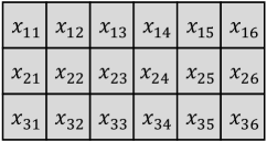
(a) Complete samples

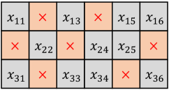
(b) Incomplete samples

Figure 1: Examples of complete and incomplete data with dimension 6.

However, note that in the framework of GAIN [43], only a reconstruction loss is used in the generator to minimize the imputation error of the non-missing part. It is well known that many real life datasets contain potential category information that has a close relationship with the latent feature distribution. Incorporating such information into the framework of GANs can improve the performance of the models further [20, 21, 35].

In this paper, we aim to exploit the implicit category information contained in the incomplete data, and develop a novel pseudo-label conditional GAN (PC-GAIN) to enhance the imputation quality of GAIN [43]. The starting point of our method is simple. Specifically, we first select a subset of low-missing-rate samples to perform a pre-training using the original GAIN and then synthesize their pseudo-labels by applying a clustering algorithm. Using only a subset of low-missing-rate data is critical to ensure the quality of pseudo-labels and has a crucial impact on the model’s performance (Section 4.3). Then, an auxiliary classifier is determined based on these imputed samples and the corresponding pseudo-labels. Further, the classifier is incorporated into the generative adversarial framework to help the generator to yield indistinguishable imputation results, while retaining better category information. We evaluate PC-GAIN on the UCI and MNIST datasets with various missing rates. Experimental results show that our PC-GAIN is superior to the baseline algorithms, including GAIN, especially when the missing rate is high.

The main contributions of this work are summarized as follows:

• We propose a novel conditional GAN that exploits the implicit category information contained in the incomplete data to further enhance the imputation quality of GAIN [43].

• We design an efficient pre-training procedure that only selects a part of low-missing-rate samples to perform imputation and thus improve the quality of pseudo-labels.

• An auxiliary classifier, along with the discriminator, is designed to help the generator to produce indistinguishable imputation results, while preserving better category information.

• We show that our method outperforms state-of-the-art methods in both the imputation and the prediction accuracy, especially when the missing rate is high. Moreover, regardless of the real number of categories, selecting a smaller cluster number can ensure the best performance of the model in practice, a property that makes the approach more flexible.

There are three types of missing mechanism [19]: (1) missing completely at random (MCAR); (2) missing at random (MAR), where the propensity for a data item to be missing is related to the observed data; (3) missing not at random (MNAR), where the data items are missing due to some underlying mechanisms. As in [26, 37, 43], we consider the data that are MCAR in this paper. This indicates that the missingness is caused by either unexpected external factors or control of the measurement system.

2 Related Work

2.1 Generative Adversarial Networks

A large number of neural networks have been proposed for different problems in practical applications [9, 16, 36]. Among them, generative adversarial networks (GANs) [10], a framework to construct a generative model to approximate the target distribution, have achieved state-of-the-art performance in various learning tasks [26, 27, 31, 42]. The most significant feature of GANs is the discriminator which distinguishes the difference between the generated distribution and the target distribution. The algorithm of GANs iteratively trains the discriminator and generator, where the discriminator acts as an increasingly rigorous criticism of the current generator. However, the original GANs do not use additional information such as labels to monitor the training, and thus may lose important patterns in the generated results.

Conditional GANs (cGANs) [25] can be regarded as an augmentation of GANs that use conditional information such as labels to improve the discriminator and generator. Conditional GANs have been popularly used in conditional image synthesis [41], the generation of the images from text [33], and image to image translation [14]. Unlike original GANs, the discriminator of cGANs discriminates between the generator distribution and the target distribution on the set of generated samples and its conditional variable. However, in practice, it is often expensive to obtain actual labels for large-scale datasets. Therefore, for unlabeled or partially labeled data, one solution is to modify the discriminator to predict the class distribution [30, 38] or a subset of latent variables from which the samples are generated [6]. Another solution is to train class-conditional GANs on unlabelled data by clustering on features obtained by unsupervised learning methods [20, 21, 35].

2.2 Deep Generative Imputation Methods

Traditional methods for missing data imputation usually assumes a linear relationship between the observed part and the missing part of the data, However, such linear relationship usually does not exist in reality. Because of the strong nonlinear fitting ability of neural networks, there has been a surge of interest in developing deep generative models for missing data imputation. For example, Gondara and Wang [9] considered a multiple imputation model based on overcomplete deep denoising autoencoders. Tran et al. [39] proposed a cascade residual automatic encoder(CRA) which compensates for missing data by utilizing the correlation between different modalities. Mattei [22] presented an importance-weighted autoencoder that maximises a potentially tight lower bound of the log-likelihood of the observed data. Nazabal et al. [29] proposed a general framework of variational autoencoders that effectively incorporates incomplete data and heterogenous observations. Spinelli et al. [37] formulated the missing data imputation task in terms of a graph denoising autoencoder, where each edge of the graph encodes the similarity between two patterns.

Imputation methods using GAN frameworks have also been proposed. Pathak et al. [32] presented context encoders using a pixel-wise reconstruction loss plus an adversarial loss to generate the contents of an arbitrary image region conditioned on its surroundings. Xu et al. [42] presented a tabular GAN where the generator outputs variable values in an ordered sequence using a recurrent neural network architecture. Mottini et al [26] handled PNRs data with missing values by use of a Cramer GAN [3], where feedforward layers with the Cross-Net architecture and an input embedding layer for the categorical features are added. Yoon et al. [43] proposed a generative adversarial imputation network (GAIN) for missing data imputation, where the generator outputs a completed vector conditioned on what is actually observed, and the discriminator attempts to determine which entries in the completed data were observed and which were imputed. Li et al. [18] introduced an auxiliary GAN for learning a mask distribution to model the missingness. The complete data generator is trained so that the resulting masked data are indistinguishable from real incomplete data that are masked similarly. However, training two generative adversarial networks at the same time can be quite computationally complex. Moreover, the generative imputation models mentioned above have not considered the use of implicit category information to improve the imputation performance.

3 Pseudo-label conditional GAIN

Let $\mathbf{\chi}=\{\mathbf{x}^{1},\mathbf{x}^{2},\cdots,\mathbf{x}^{N}\}\in\mathbb{R}^{d}$ denote an incomplete dataset. For each $\mathbf{x}\in\mathbf{\chi}$, there is a corresponding binary mask vector $\mathbf{m}=\{0,1\}^{d}$, where $m_{i}=1$ if the feature $x_{i}$ is observed, and $m_{i}=0$ if $x_{i}$ is missing.

3.1 The Review of GAIN

In [43], the authors proposed a generative adversarial neural network called GAIN to impute the missing values. In GAIN, the generator $G$ takes the incomplete sample $\mathbf{x}$, the mask vector $\mathbf{m}$ and a source of noise as input and output the complete sample, and then the discriminator $D$ tries to distinguish which entries are observed and which are imputed. Further, to alleviate the diversity of the solution, a hint mechanism was introduced to provide additional missing information for the discriminator.

Specifically, the output of the generator $G$ in GAIN could be denoted by

$$\mathbf{x}_{G}=G(\mathbf{x},\mathbf{m},(1-\mathbf{m})\odot\mathbf{z}),$$ (1)

where $\mathbf{z}$ is a $d$-dimensional noise and $\odot$ denotes the Hadamard product. The reconstructed sample is defined as

$$x_{R}=\mathbf{m}\odot\mathbf{x}+(1-\mathbf{m})\odot\mathbf{x}_{G}.$$ (2)

The output of the discriminator $D$ is an binary vector denoted by

$$\mathbf{m}_{D}=D(\mathbf{x}_{R},\mathbf{h}),$$ (3)

where $\mathbf{h}$ is a hint vector and $\mathbf{m}_{D}$ is the prediction of the mask vector $\mathbf{m}$.

The objectives of GAIN are formulated as follows

$$\begin{split}\min_{D}&\frac{1}{N}\sum_{k=1}^{N}\mathcal{L}_{D}(\mathbf{m}^{k},\mathbf{m}_{D}^{k}),\\[5.0pt] \min_{G}&\frac{1}{N}\sum_{k=1}^{N}\left(\mathcal{L}_{G}(\mathbf{m}^{k},\mathbf{m}_{D}^{k})+\alpha\mathcal{L}_{R}(\mathbf{x}^{k},\mathbf{x}_{R}^{k})\right),\end{split}$$ (4)

where $\alpha$ is a weight parameter, $\mathcal{L}_{D}$ is a cross entropy loss term such that

$$\mathcal{L}_{D}(\mathbf{m},\mathbf{m}_{D})=-\mathbf{m}\log\mathbf{m}_{D}-(1-\mathbf{m})\log(1-\mathbf{m}_{D}),$$ (5)

$\mathcal{L}_{G}$ is defined as

$$\mathcal{L}_{G}(\mathbf{m},\mathbf{m}_{D})=-(1-\mathbf{m})\log\mathbf{m}_{D},$$ (6)

and $\mathcal{L}_{R}$ is a reconstruction loss satisfying

$$\mathcal{L}_{R}(\mathbf{x},\mathbf{x}_{R})=\sum_{i=1}^{d}m_{i}L_{R}(x_{i},x_{R,i}),$$ (7)

with

$$L_{R}(x_{i},x_{R,i})=\left\{\begin{array}[]{ll}(x_{i}-x_{R,i})^{2},&\text{for numerical variable}\\[5.0pt] -x_{i}\log x_{R,i},&\text{for categorial variable}\end{array}\right..$$ (10)

3.2 Formulation of PC-GAIN

It is well known that the conditional information such as labels can enhance the performance of the generator [20, 25]. However, applying the existing conditional techniques to common imputation problems mainly faces two difficulties. First, most imputation problems are completely unsupervised and there are no explicit labels could be used directly. Secondly, since the data are incomplete, it is particularly difficult to synthesize appropriate pseudo-labels for the samples.

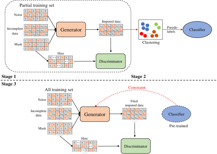
Figure 2: An overview of the proposed PC-GAIN.

In this section, we would like to propose a novel algorithm based on GAIN to solve the above difficulties. Figure 2 shows the whole framework of the proposed method. We first select low-missing-rate samples to pre-train the generator $G$ and the discriminator $D$ to obtain the imputed dataset. Then, a clustering algorithm is applied on the imputed dataset to synthesize the pseudo-labels. And we train a classifier with imputed dataset and pseudo-labels. Finally, we use all training data to train the generator $G$ and the discriminator $D$, and simultaneously use the pre-trained classifier to constrain the generator. The details of the proposed method are described in the following.

First, note that even under a fixed missing rate, the missingness of each sample in a dataset is different. In our opinion, the potential category information contained in those low-missing-rate samples is more reliable. Therefore, we would like to select a subset of low-missing-rate samples to conduct a pre-training procedure. The aim of the pre-training is to impute the missing components of these low-missing-rate data and then deduce their pseudo-labels.

Specifically, for any $\mathbf{x}$, we calculate its missing rate $r(\mathbf{x})$ as follows

$$r(\mathbf{x})=\frac{1}{d}\sum_{i=1}^{d}m_{i}.$$ (11)

where $\mathbf{m}$ is the mask vector of the data. Then we sort all samples in an ascending order according to their missing rates, and choose the first $\lambda N$ ( $0<\lambda<1$) samples to formulate a pre-training dataset $\chi^{L}$. Following the optimization objectives (4), we pre-train the generator $G$ and the discriminator $D$ using the dataset $\chi^{L}$. After then, we can obtain an imputed dataset denoted as $\chi_{R}^{L}$ of the dataset $\chi^{L}$.

To synthesize the pseudo-labels $\{\mathbf{p}_{R}^{L}\}$ of these low-missing-rate data, we can apply a clustering algorithm, e.g. [2, 21, 27], on the imputed dataset $\chi_{R}^{L}$. It is worth to point out that the number of the clusters is not need to be consistent with the number of the real categories. In our experiments, we found that for many UCI datasets, a small value of $K$ between 4 and 6 is enough to ensure the best performance of the model.

Next, we use $\chi_{R}^{L}=\{\mathbf{x}_{R}^{L}\}$ and the corresponding pseudo-labels $\{\mathbf{p}_{R}^{L}\}$ to train an auxiliary classifier $C$. With the aid of this classifier, we update the generator $G$ and discriminator $D$ again. That is, we require the generator not only outputs indistinguishable imputed data, but also learns distinct categorical characteristics. More specifically, the objectives of the discriminator and the generator now become

$$\begin{split}\min_{D}&\frac{1}{N}\sum_{k=1}^{N}\mathcal{L}_{D}(\mathbf{m}^{k},\mathbf{m}_{D}^{k}),\\[5.0pt] \min_{G}&\frac{1}{N}\sum_{k=1}^{N}\left(\mathcal{L}_{G}(\mathbf{m}^{k},\mathbf{m}_{D}^{k})+\alpha\mathcal{L}_{R}(\mathbf{x}^{k},\mathbf{x}_{R}^{k})+\beta\mathcal{L}_{C}(\mathbf{x}_{R}^{k})\right),\end{split}$$ (12)

where $\alpha$ and $\beta$ are hyperparameters, and $L_{C}$ is a standard information entropy loss such that

$$\mathcal{L}_{C}(\mathbf{x}_{R})=-C(\mathbf{x}_{R})\log C(\mathbf{x}_{R}),$$ (13)

with $C(\mathbf{x}_{R})$ denoting the output of the auxiliary classifier.

Note that the main difference between (4) and (12) is that in the objectives of PC-GAIN, an additional entropy loss $L_{C}$ is introduced to promote the model to learn more distinct categorical features. This loss is determined by the auxiliary classifier $C$, which is only pre-trained on a subset $\{\mathbf{x}_{R}^{L},\mathbf{p}_{R}^{L}\}$, and fixed during the training of the generative adversarial network. Hence, this additional classier will not increase the training complexity of the GANs. The pseudo-code for our PC-GAIN is shown in Algorithm 1.

Algorithm 1 Pseudo-Code of PC-GAIN

Input: Incomplete dataset $\chi$, number of clusters $K$ and proportion parameter $\lambda$.

Pre-training

1:Sort all data in an ascending manner according to their missing rates.

2:Select the top $\lambda$ ($0<\lambda<1$) of the data to formulate a pre-training dataset $\chi^{L}$.

3:Use $\chi^{L}$ and the objectives (4) to train the discriminator $D$ and the generator $G$.

Determine the pseudo-labels and the classifier $C$

1:Cluster the imputed results of the first stage and synthesize the pseudo-labels for these data.

2:Train a classifier $C$ using the imputed data and their pseudo-labels.

Updata the generator $G$ and the discriminator $D$

1:Use the whole dataset $\chi$ and the new objectives (12) to train the discriminator $D$ and the generator $G$ again.

4 Experiments

4.1 Experimental Setup

4.1.1 Datasets

In this section, we evaluate the performance of PC-GAIN on six datasets from the UCI repository [7] and the MNIST dataset [17], respectively. The details of the UCI datasets are listed in Table 1.

Table 1: The basic properties of the UCI datasets

Dataset	Samples	Numerical variables	Categorial variables	Number of classes
BalanceScale	625	0	4	3
BreastCancer	569	30	0	2
CarEvaluation	1728	0	6	4
Credit	30000	14	9	2
Letter	20000	16	0	26
News	39797	35	23	2
Spam	4601	57	0	2
WineQuality(white)	4898	11	0	7

Since no dataset contains missing values originally, for a given missing rate, we remove the features of all data completely at random to formulate an incomplete dataset. Moreover, each variable is scaled to the interval $[0,1]$.

4.1.2 Compared Methods and Experimental Settings

We shall compare PC-GAIN with a range of baseline methods, including Autoencoder [9], EM [8], MissForest [4], MICE [5] and GAIN [43]. Among them, MissForest and MICE belong to classical benchmark discriminative models, while Autoencoder, EM and GAIN are generative methods. To make a fair comparison of PC-GAIN and GAIN, we adopt the same generative adversarial network architecture as [43]. We take 5-cross validation in our experiments. Each experiment is repeated ten times and the average performance is reported.

Unless stated otherwise, the performance of each model is evaluated under a 50% missing rate, the weight parameters in (12) are chosen as $\alpha=200$ and $\beta=20$, and the number of clusters $K=5$. We use $\lambda=0.2$ for three bigger datasets: Credit, Letter and News, and $\lambda=0.4$ for others.

In our PC-GAIN, the auxiliary classifier is a three-layer fully connected neural network (NN) using ReLU activation. The number of neurons in each hidden layer is the same as the input dimension of the data. We apply the KMeans++ clustering [2] on the original imputation results of the UCI data, while for the MNIST dataset, we apply KMeans++ to cluster the latent feature space of the generator.

4.2 Imputation Accuracy in UCI Datasets

RMSE is a commonly used metric for evaluating the performance of missing data imputation, which computes the root mean square error of the imputed missing values against the ground truth.

Table 2: Comparisons with state-of-the-art methods on the UCI datasets. RMSE under a 50% missing rate.

	BalanceScale	BreastCancer	CarEvaluation	Credit	Letter	News	Spam	WineQuality
Autoencoder [9]	0.4788	0.1148	0.4814	0.1932	0.2216	0.2726	0.0957	0.1814
EM [8]	0.4992	0.1176	0.5492	0.1923	0.2183	0.3064	0.0737	0.1520
MissForest [4]	0.4322	0.1073	0.4784	0.1817	0.1905	0.2633	0.0673	0.1597
MICE [5]	0.5161	0.1158	0.5521	0.1843	0.1714	0.2763	0.1062	0.1304
GAIN [43]	0.4148	0.0944	0.4343	0.1832	0.1587	0.2532	0.0583	0.1397
PC-GAIN	0.3754	0.0939	0.4227	0.1616	0.1450	0.2269	0.0559	0.1323

We first report RMSE of PC-GAIN and the baseline models in Table 2. It can be seen that, except that it is slightly worse than the MICE method on the WineQuality dataset, the performance of PC-GAIN outperforms the benchmark methods on most datasets.

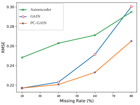
(a) News

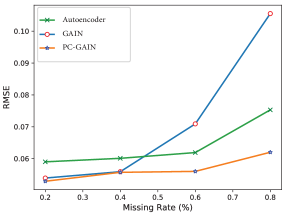
(b) Spam

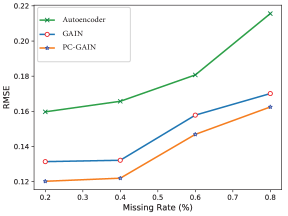
(c) Winequality

Figure 3: RMSE of PC-GAIN versus AutoEncoder and GAIN with various missing rates.

Next, we use News, Spam and WineQualy as examples to illustrate the performance of PC-GAIN under various missingness. As shown in Figure 3, PC-GAIN consistently outperforms the compared models under various missingness. Especially, the advantage becomes more obvious when the missing rate becomes higher.

4.3 Prediction Performance under Various Missing Rates

It is a common understanding that a good imputation model should not only restore the data accurately, but also maintain the category information of the data. In this section, we compare PC-GAIN against other two deep generative models: Autoencoder [9] and GAIN [43], with respect to the accuracy of post-imputation prediction. We use a same classifier (a two-layer fully connected network with Softmax activation) for all three modes.

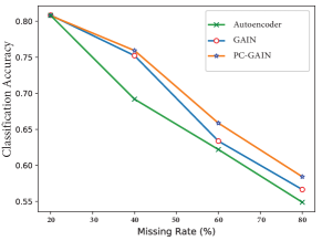
(a) News

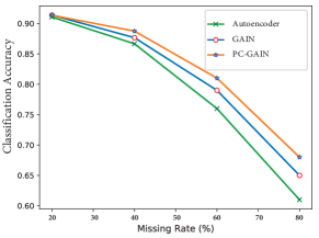
(b) Spam

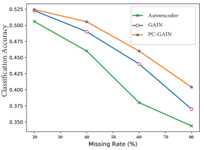
(c) Winequality

Figure 4: Post-imputation prediction accuracy of PC-GAIN versus AutoEncoder and GAIN with various missing rates.

It is observed from Figure 4 that PC-GAIN achieves the best classification accuracy in all cases. Moreover, the improvements in prediction accuracy become more significant as the missing rate increases. This phenomenon, with the imputation accuracy shown in Figure 3, implies that PC-GAIN is a reliable imputation method especially in the case of high missing rate.

4.4 Sensitivity Analysis

This section evaluates the performance of PC-GAIN under various configurations.

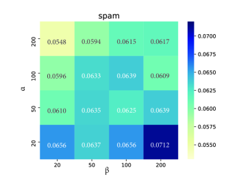
(a) Spam

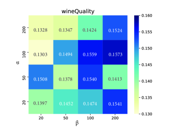
(b) WineQuality

Figure 5: RMSE of PC-GAIN with various $\alpha$ and $\beta$.

First, we investigate the influences of the weight parameters $\alpha$ and $\beta$ in the objectives (12). We use a heat map manner to depict RMSE of PC-GAIN with various weights. As shown in Figure 5, compared with $\alpha$, a relative smaller $\beta$ can yield better results. This implies that in the framework of PC-GAIN, the classifier loss has a greater impact on the imputation quality than the discriminator.

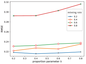
(a) News

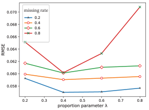
(b) Spam

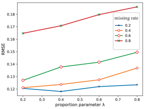
(c) WineQuality

Figure 6: The influence of the proportion parameter $\lambda$.

In the pre-training stage, there is a proportion parameter $\lambda$, which controls the number of selected data in pre-training. Next, we examine the effect of this parameter.

We can see from Figure 6 that $\lambda$ has a decisive effect on the quality of imputation. The performance of PC-GAIN deteriorates rapidly when $\lambda$ becomes too large. This is most likely because too many incomplete data may increase the unreliability of pseudo-labels, and thus reduces the quality of the imputation. We also find that the optimal choice of $\lambda$ for UCI datasets is usually below than 0.4.

Finally, we examine the influence of the number of clusters. From Figure 7, we can observe that the performance of PC-GAIN is stable with respect to the number of clusters. In most cases, PC-GAIN achieves a better results when $K$ belonging 4 to 8, regardless of the true number of categories. This property is very desirable, because in practice we only need to consider a small $K$ even if the actual number of categories is large, and thus save the computational overhead.

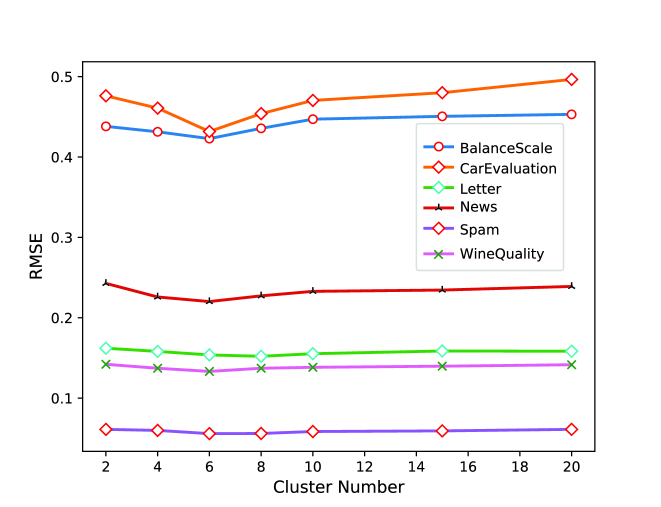
Figure 7: RMSE of PC-GAIN with various number of clusters.

4.5 Imputation Accuracy under Various Clustering and Classification Methods

The proposed PC-GAIN utilized a clustering algorithm and an auxiliary classifier to improve the GAIN. In this section, we analyze the relationship between the final imputation results and the classification and clustering methods used.

The classification methods adopted in the analysis are as follows: Multiclass SVM [13] (has high classification accuracy), a fully-trained neural network classifier (has high classification accuracy), a little-trained neural network classifier (has low classification accuracy), and a no-trained neural network classifier(completely random classification). The clustering methods used in this analysis are: KM(KMeans) [11], SC (SpectralClustering) [40], KMPP(KMeans++) [2], and AC(AgglomerativeClustering) [28]. Two quantitative indicators Ca (Calinski Harabasz) [23] and Si (Silhouette Coefficient) [34] are used to measure the quality of clustering. The higher the value of these indicators, the better.

Table 3 shows the imputation results under various clustering and classification methods on two toy datasets and a realistic UCI dataset, where the baseline denotes the result of the original GAIN. Square is a two-dimensional toy data with four categories, and the data of each category is strip distribution [15]. Twomoons is a classic double moon shape data [44]. News comes from the UCI dataset. RMSE is used to evaluate the imputation results. The lower the RMSE value, the better.

Table 3: Comparison of imputation results under various clustering and classification methods.

Dataset		Multiclass-SVM	NN(complete train)	NN(moderate train)	NN(not train)
	Baseline	0.3545
	KM(Ca:228.4733 , Si:0.5778)	0.2611	0.2657	0.3277	0.3580
Square	SC(Ca:241.5169 , Si:0.6295)	0.2454	0.2512	0.3143	0.3538
	KMPP(Ca:231.5886 , Si:0.5862)	0.2528	0.2530	0.3017	0.3497
	AC(Ca:234.0248 , Si:0.6024)	0.2577	0.2615	0.3225	0.3585
	Baseline	0.3230
	KM(Ca:437.2172 , Si:0.4808)	0.2592	0.2591	0.2892	0.3227
Twomoons	SC(Ca:422.9569 , Si:0.4697)	0.2506	0.2405	0.2749	0.3308
	KMPP(Ca:361.1315 , Si:0.4355)	0.2501	0.2499	0.2908	0.3172
	AC(Ca:410.3813 , Si:0.4586)	0.2583	0.2510	0.2738	0.3099
	Baseline	0.2532
	KM(Ca:259.7938 , Si:0.2165)	0.2209	0.2269	0.2340	0.2774
News	SC(Ca:244.6607 , Si:0.2136)	0.2228	0.2253	0.2297	0.2674
	KMPP(Ca:194.9008 , Si:0.1829)	0.2256	0.2269	0.2390	0.2705
	AC(Ca:190.7064 , Si:0.1936)	0.2222	0.2227	0.2358	0.2644

Each column in the Table 3 reflects the imputation results of different clustering methods and a certain classification method, and each row in the Table 3 reflects the imputation results of a certain clustering method and different classification methods. As can be seen from Table 3 (all rows and the first two columns), the model has strong robustness for various clustering methods and classification methods on each dataset. Although different clustering methods have different effects on a dataset, when the clustering results are fully learned by the classifiers, they can be used to guide the network to impute the missing data. As can be seen from the last three columns of the Table 3, when the classifier has not been fully trained, the classification accuracy is low, and the classifier’s supervisory role on the imputation network is weak at this time. However, with the continuous training of the classifier, the classification accuracy increases, and the ability of the classifier to supervise the imputation network is also gradually enhanced, so that the imputation network can output more reliable imputed results.

4.6 Image Inpainting

In this section, we show that PC-GAIN can also improve the performance of GAIN in image inpainting task. To this end, we consider the MNIST dataset [17]. For each image in MNIST, we remove 50% and 80% pixels uniformly at random. We compare the imputation results using FID index [12]. FID represents the distance between the eigenvectors of the generated image and the eigenvectors of the real image, a lower FID value often means that the generated image is closer to the real image.

It is obvious from Figures 8 and 9 that the imputed images of PC-GAIN are more cohesive and smoother than those of GAIN. Moreover, the output of PC-GAIN has a lower FID value at both cases, and the advantage becomes greater at a higher miss rate.

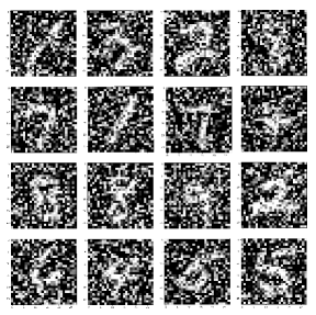
(a) Incomplete image

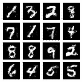
(b) GAIN (FID 1.721)

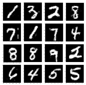
(c) PC-GAIN (FID 1.551)

Figure 8: Imputed images on MNIST under a 50% missing rate

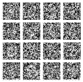
(a) Incomplete image

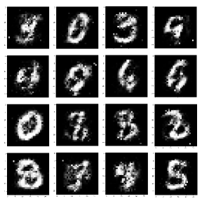
(b) GAIN (FID 5.642)

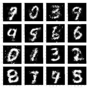
(c) PC-GAIN(FID 4.520)

Figure 9: Imputed images on MNIST under a 80% missing rate

5 Concluding Remarks

Based on the recent work of [43], we propose a novel generative model called PC-GAIN for missing data imputation. With the aid of an auxiliary classifier, which has been pre-trained using a subset of low-missing-rate samples and the corresponding pseudo-labels, the generator tries to produce indistinguishable imputation results that have obvious categorical characteristics. It is worth noting that this classifier is always fixed during the training of generative adversarial networks, so the proposed method is easy to implement. On the whole, PC-GAIN can be regarded as an improved version of GAIN [43], which promotes the performance of the original model significantly without using any supervision, especially under a high missing rate.

The key of PC-GAIN is to exploit the potential category information contained in the missing data to enhance the imputation results. This novel idea is very general and can be applied to other existing frameworks, as long as the potential category information can be accurately captured. However, compared with traditional and other deep learning methods, an additional pre-training step is needed in our framework, which requires more time in training process and has a larger number of hyperparameters to be adjusted.

Although we only focus on the MCAR case in this paper, our approach can be extended to handle both MAR and MNAR mechanisms. Note that the selected pre-training subset has an important impact on the quality of the pseudo-labels, and thereby affects the imputation results. For MAR, we can still pre-train some low-missing-rate data to ensure the quality of the pseudo-labels. However, for MNAR, it is not a good idea to simply select a subset with low missingness, which may lead to selection bias and reduce the accuracy of the pseudo-labels. A more suitable pre-training subset should be chosen according to the corresponding missing mechanism. It will be a meaningful work to apply the main idea of PC-GAIN in other frameworks to deal with MNAR case.

Acknowledgments. This research is partially supported by National Natural Science Foundation of China (11771257) and Natural Science Foundation of Shandong Province (ZR2018MA008)

References

- [1] Abiri N., Linse B., Edén P. & Ohlsson M. (2019) Establishing strong imputation performance of a denoising autoencoder in a wide range of missing data problems. Neurocomputing, 365:137–146.
- [2] Arthur D. & S. Vassilvitskii S. (2007) K-means++: The advantages of careful seeding. In Proceedings of the Annual ACM-SIAM Symposium on Discrete Algorithms (ACM).
- [3] Bellemare M.G., Danihelka I., Dabney W., Mohamed S., Lakshminarayanan B., Hoyer S. & Munos R. (2018) The cramer distance as a solution to biased wasserstein gradients. In International Conference on Learning Representations (ICLR).
- [4] Buhlmann P. (2012) MissForest: non-parametric missing value imputation for mixed-type data. Bioinformatics, 28:112–118.
- [5] van Buuren S. & Groothuis-Oudshoorn K. (2011) MICE: Multivariate imputation by chained equations in R. Journal of Statistical Software, 45:1–67.
- [6] Chen X., Duan Y., Houthooft R., Schulman J., Sutskever I. & Abbeel P. (2016) InfoGAN: Interpretable representation learning by information maximizing generative adversarial nets. In Advances in Neural Information Processing Systems (NIPS).
- [7] Dua D. & Graff C. (2017) UCI Machine Learning Repository.
- [8] Garíca-Laencina P., Sancho-Gómez J. & Figueiras-Vidal A. (2010) Pattern classification with missing data: a review. Neural Comput. Appl., 19:263–282.
- [9] Gondara L. & Wang K. (2017) Multiple imputation using deep denoising autoencoders. arXiv preprint arXiv:1705.02737.
- [10] Goodfellow I., Pouget-Abadie J., Mirza M., Xu B., Warde-Farley D., Ozair S., Courville A. & Bengio Y. (2014) Generative adversarial nets. In Advances in Neural Information Processing Systems (NIPS).
- [11] Hartigan J.A., & Wong M.A. (1979) A K-means clustering algorithm. Journal of the Royal Statistical Society: Series C (Applied Statistics), 28(1): 100-108.
- [12] Heusel M., .Ramsauer H., Unterthiner T., Nessler B. & Hochreiter S. (2017) GANs trained by a two time-scale update rule converge to a local Nash equilibrium. In Advances in Neural Information Processing Systems (NIPS).
- [13] Hsu, C.W., & Lin, C.J. (2002) A comparison of methods for multiclass support vector machines. IEEE transactions on Neural Networks, 13(2), 415–425.
- [14] Isola P., Zhu J., Zhou T. & Efros A. (2017) Image-to-image translation with conditional adversarial networks. In IEEE Conference on Computer Vision and Pattern Recognition (CVPR).
- [15] Jain A.K., Murty M.N., & Flynn P.J. (1999) Data clustering: a review. ACM Computing Surveys (CSUR), 31(3), 264–323.
- [16] Kiranyaz, S., Ince, T., Iosifidis, A., & Gabbouj, M. (2020) Operational neural networks. Neural Comput. Appl., 32, 6645–6668.
- [17] LeCun Y. & Cortes C. (2010) MNIST Handwritten Digit Database.
- [18] Li C., Jiang B. & Marlin B. (2019) MisGAN: learning from incomplete data with generative adversarial networks. In International Conference on Learning Representations (ICLR).
- [19] Little R.J. & Rubin D.B. (2019) Statistical analysis with missing data, Third Edition. John Wiley and Sons.
- [20] Liu S., Wang T., Bau D., Zhu J. & A.Torralba A. (2020) Diverse image generation via self-conditioned GANs. In IEEE Conference on Computer Vision and Pattern Recognition (CVPR).
- [21] Lucic M., Tschannen M., Ritter M., Zhai X., Bachem O. & Gelly S. (2019) High-fidelity image generation with fewer labels. In International Conference on Machine Learning (ICML).
- [22] Mattei P.A. & J. Frellsen J. (2019) MIWAE: deep generative modelling and imputation of incomplete data. In International Conference on Machine Learning (ICML).
- [23] Maulik U. & Bandyopadhyay S. (2002) Performance evaluation of some clustering algorithms and validity indices. IEEE Transactions on Pattern Analysis and Machine Intelligence, 24(12), 1650-1654.
- [24] Mazumder R., Hastie T. & Tibshirani R. (2009) Spectral regularization algorithms for learning large incomplete matrices. Journal of Machine Learning Research, 11:2287.
- [25] Mirza M. & Osindero S. (2014) Conditional generative adversarial nets. arXiv preprint arXiv:1411.1784.
- [26] Mottini A., Lheritier A. & Acuna-Agost R. (2018) Airline passenger name record generation using generative adversarial networks. arXiv preprint arXiv:1807.06657.
- [27] Mukherjee S., Asnani H., Lin E. & Kannan S. (2019) ClusterGAN: latent space clustering in generative adversarial networks. In Proceedings of the AAAI Conference on Artificial Intelligence (AAAI).
- [28] Murtagh F. & Contreras P. (2012) Algorithms for hierarchical clustering: an overview. Wiley Interdisciplinary Reviews: Data Mining and Knowledge Discovery, 2(1): 86-97.
- [29] Nazabal A. Olmos P., Ghahramani Z. & Valera I. (2020) Handling incomplete heterogeneous data using VAEs. Pattern Recognition, 107:107501.
- [30] Odena A., Olah C. & Shlens J. (2017) Conditional image synthesis with auxiliary classifier GANs. In International Conference on Machine Learning (ICML).
- [31] Ortaç G., Doğan Z., Orman Z., & Şamli R. (2020) Baby face generation with generative adversarial neural networks: a case study. Acta Infologica, 4(1), 1-9.
- [32] Pathak D., Krahenbuhl P., Donahue J., Darrell T. & Efros A. (2016) Context encoders: feature learning by inpainting. In IEEE Conference on Computer Vision and Pattern Recognition (CVPR).
- [33] Reed S., Akata Z., Yan X., Logeswaran L., Schiele B.& Lee H. (2016) Generative adversarial text to image synthesis. arXiv preprint arXiv:1605.05396.
- [34] Rousseeuw P.J. (1987) Silhouettes: a graphical aid to the interpretation and validation of cluster analysis. J. Comput. Appl. Math, 20, 53-65.
- [35] Sage A., Agustsson E., Timofte R. & Gool L.V. (2018) Logo synthesis and manipulation with clustered generative adversarial networks. In IEEE Conference on Computer Vision and Pattern Recognition (CVPR).
- [36] Sevgen, S., Arslan, E., & Samli, R. (2017) Solving SUDOKU puzzle with numbers recognized by using artificial neural networks. Istanbul University-Journal of Electrical & Electronics Engineering, 17(1), 3239-3247.
- [37] Spinelli I., Scardapane S. & Uncini A. (2020) Missing data imputation with adversarially-trained graph convolutional networks. Neural Networks, 129:249–260.
- [38] Springenberg J.T. (2015) Unsupervised and semi-supervised learning with categorical generative adversarial networks. arXiv preprint arXiv:1511.06390.
- [39] Tran L., Liu X., Zhou J. & Jin R. (2017) Missing modalities imputation via cascaded residual autoencoder. In IEEE Conference on Computer Vision and Pattern Recognition (CVPR).
- [40] Von Luxburg U. (2007) A tutorial on spectral clustering. Statistics and Computing, 17(4):395-416.
- [41] Wang T., Liu M., Zhu J., Tao A., Kautz J. & Catanzaro B. (2018) High-resolution image synthesis and semantic manipulation with conditional GANs. In IEEE Conference on Computer Vision and Pattern Recognition (CVPR).
- [42] Xu L. & Veeramachaneni K. (2018) Synthesizing tabular data using generative adversarial networks. arXiv preprint arXiv:1811.11264.
- [43] Yoon J., Jordon J. & van der Schaar M. (2018) Gain: Missing data imputation using generative adversarial nets. In International Conference on Machine Learning (ICML).
- [44] Zhou D., Bousquet O., Lal T.N, Weston J. & SchÖlkopf B. (2004) Learning with local and global consistency. In Advances in Neural Information Processing Systems (NIPS).