Universality classes of the Anderson Transitions Driven by non-Hermitian Disorder

Abstract

An interplay between non-Hermiticity and disorder plays an important role in condensed matter physics. Here, we report the universal critical behaviors of the Anderson transitions driven by non-Hermitian disorders for three dimensional (3D) Anderson model and 3D U(1) model, which belong to 3D class ${\rm AI}^{\dagger}$ and 3D class A in the classification of non-Hermitian systems, respectively. Based on level statistics and finite-size scaling analysis, the critical exponent for length scale is estimated as $\nu=0.99\pm 0.05$ for class ${\rm AI}^{\dagger}$, and $\nu=1.09\pm 0.05$ for class A, both of which are clearly distinct from the critical exponents for 3D orthogonal and 3D unitary classes, respectively. In addition, spectral rigidity, level spacing distribution, and level spacing ratio distribution are studied. These critical behaviors strongly support that the non-Hermiticity changes the universality classes of the Anderson transitions.

Introduction— Continuous quantum phase transitions are universally characterized by critical exponent (CE) and scaling functions for physical observables around the critical point Sondhi et al. (1997). The CE and scaling functions represent scaling properties of an underlying effective theory that describes the phase transition, and classify the phase transitions in different models in terms of the universality class. The universality class of the Anderson transition (AT) Anderson (1958) is determined only by the spatial dimension and symmetry of a system Abrahams et al. (1979); Wegner (1976); Effetov et al. (1980); Hikami et al. (1980); Hikami (1981); Altland and Zirnbauer (1997); Evers and Mirlin (2008); Kramer and MacKinnon (1993); Slevin and Ohtsuki (2014, 1997, 2016); Asada et al. (2005); Slevin and Ohtsuki (2009); Asada et al. (2004); Luo et al. (2018, 2020). Recently, the AT in non-Hermitian (NH) system attracts a lot of attentions Xu et al. (2016); Tzortzakakis et al. (2020); Wang and Wang (2020); Huang and Shklovskii (2020a, b). NH systems and localization phenomena therein are remarkably ubiquitous in nature, such as random lasers Cao et al. (1999); Wiersma (2008, 2013), non-equilibrium open systems with gain and/or loss Konotop et al. (2016); Feng et al. (2017); El-Ganainy et al. (2018); Ozdemir et al. (2019); Miri and Alù (2019), and correlated quantum many-particle systems of quasiparticles with finite life-time Shen and Fu (2018); Papaj et al. (2019). Hatano and Nelson’s pioneering work introduced a one-dimensional (1D) NH Anderson model with asymmetric hopping potentials Hatano and Nelson (1996). The 1D NH model shows a delocalization-localization transition, contrary to the absence of the AT in 1D Hermitian system, indicating that the transition belongs to a new universality class Kawabata and Ryu (2020). According to recent studies, the non-Hermiticity enriches the ten-fold classification scheme of the Hermitian system by Altland and Zirnbauer Altland and Zirnbauer (1997) into 38-fold symmetry classes Kawabata et al. (2019); Zhou and Lee (2019).

A natural question arises whether the AT in each of these 38-fold symmetry classes in the NH system belongs to a new universality class or not, compared with the known universality classes in the Hermitian system. A recent work Xu et al. (2016) shows that a NH spin ice model belongs to the same universality class as two-dimensional (2D) quantum Hall universality class of the Hermitian system. Another recent work Huang and Shklovskii (2020a) indicates the CE $\nu$ of three-dimensional (3D) NH Anderson model to be the same as the CE of the Hermitian Anderson model Huang and Shklovskii (2020a). These works, at first sight, suggest that the non-Hermiticity does not change the universality class of the AT, and the AT in the NH system with the enriched symmetry classes share the same universal critical properties as the AT in the corresponding symmetry classes in the Hermitian system.

In this paper, we show that the non-Hermiticity does change the universality class of the AT. By precise estimates of the CE $\nu$ as well as critical level statistics such as spectral compressibility, level spacing distribution and level spacing ratio (LSR) distribution, the universal critical properties of the AT in the NH systems are shown to be significantly different from any of the Hermitian symmetry classes. Here, two symmetry classes are studied as an example; 3D class AI^† and 3D class A in the NH classification scheme. By an accurate calculation of the LSR Oganesyan and Huse (2007); Sá et al. (2020); Huang and Shklovskii (2020a) and polynomial fitting of the dataSlevin and Ohtsuki (2014), $\nu$ is estimated to be $0.99\pm 0.05$ for the class AI^† and $1.09\pm 0.05$ for the class A, which are clearly distinct from the CE of the 3D AT in the orthogonal Slevin and Ohtsuki (2018) and unitary classesSlevin and Ohtsuki (2016) of the Hermitian system, respectively. We further study the spectral rigidity, level spacing distribution, and LSR distribution. These critical level statistics strongly support that non-Hermiticity changes the universality class of the AT in 3D class AI^† and 3D class A. This paper paves a solid path toward a new research paradigm of quantum phase transitions in NH systems, which will give a bridge between non-Hermitian random matrix theory and different branches in physics.

Table 1: Polynomial fitting results for the level spacing ratio (LSR) around the Anderson transition in 3D class AI^† and 3D class A models. The goodness of fit (GOF), critical disorder $W_{c}$, critical exponent $\nu$, the scaling dimension of the least irrelevant scaling variable $-y$, and the critical LSR $\langle r\rangle_{c}$ are shown for various system sizes and disorder ranges and for different orders of the Taylor expansion of the scaling function for the LSR: $(m_{1},n_{1},m_{2},n_{2})$. The square bracket is the 95% confidence interval.

Symmetry	$L$	$W$	$m_{1}$	$n_{1}$	$m_{2}$	$n_{2}$	GOF	$W_{c}$	$\nu$	$y$	$\langle r\rangle_{c}$
Class AI†	8-24	[6, 7.12]	3	3	0	1	0.11	6.28[6.26, 6.30]	1.046[1.012, 1.086]	1.75[1.65, 1.84]	0.7169[0.7163, 0.7177]
	10-24	[6, 7.19]	3	3	0	1	0.15	6.32[6.30, 6.34]	0.990[0.945, 1.040]	2.10[1.87, 2.35]	0.7155[0.7146, 0.7164]
Class A	8-24	[7, 7.56]	1	3	0	1	0.32	7.14[7.13, 7.15]	1.065[1.036, 1.100]	2.60[2.31, 2.89]	0.7178[0.7171, 0.7188]
	8-24	[7, 7.56]	2	3	0	1	0.43	7.15[7.14, 7.16]	1.068[1.034, 1.105]	2.63[2.35, 2.92]	0.7177[0.7169, 0.7186]
	8-24	[7, 7.56]	3	3	0	1	0.49	7.15[7.14, 7.16]	1.065[1.031, 1.103]	2.64[2.35, 2.92]	0.7177[0.7169, 0.7186]
	10-24	[6.8, 7.6]	3	3	0	1	0.12	7.14[7.12, 7.16]	1.091[1.050, 1.151]	2.50[1.88, 3.16]	0.7187[0.7170, 0.7201]

Model and numerical method— We study the following tight-binding model on a 3D cubic lattice,

$${\cal H}=\sum_{i}\varepsilon_{i}c_{i}^{\dagger}c_{i}+\sum_{\langle i,j\rangle}e^{2\pi i\cdot\theta_{i,j}}c_{i}^{\dagger}c_{j},$$ (1)

where $c_{i}^{\dagger}$ ($c_{i}$) is the creation (annihilation) operator, and $\langle i,j\rangle$ means the nearest neighbor sites with $\theta_{i,j}=-\theta_{j,i}$. The AT driven by real-valued random potentials $\varepsilon_{i}$ belongs to the 3D orthogonal universality class with $\theta_{i,j}=0$ and 3D unitary universality class with $\theta_{i,j}$ random number in $[0,1)$. In this paper, we consider NH disorder, set $\varepsilon_{j}=w_{j}^{r}\,+\,i\,w_{j}^{i}$ with the imaginary unit $i$, where $w_{j}^{r}$ and $w_{j}^{i}$ are independent random numbers with identical uniform distribution in $[-W/2,W/2]$ at site $j$. Hence ${\cal H}\neq{\cal H}^{\dagger}$. The NH random potentials can be physically realized in random lasers in random dissipation and amplification region Cao et al. (1999); Wiersma (2008, 2013). According to the symmetry classification for NH system Kawabata et al. (2019); Zhou and Lee (2019), the model belongs to 3D class AI^† with $\theta_{i,j}=0$ and 3D class A with $\theta_{i,j}$ random number in $[0,1)$. The time reversal symmetry (TRS) is broken (${\cal H}^{*}\neq{\cal H}$) in the both classes, whereas the transposition symmetry (${\cal H}^{\rm T}={\cal H}$), namely TRS^†, holds true in the class AI^†.

The AT can be characterized by the energy level statistics Wigner (1951); Dyson (1962a, b). The level statistics in NH disordered systems are known in the two limiting cases; it belongs to the Poisson ensemble in the localized phase Grobe et al. (1988), while it belongs to the Ginibre ensemble in the delocalized phase Ginibre (1965). In this paper, we analyze scaling behaviors Shklovskii et al. (1993) of the energy level statistics Wigner (1951); Dyson (1962a, b) around the AT in the NH systems, where a narrow energy window $\{E_{i}\}$ is set with an assumption that all eigenstates within the energy window have a similar critical disorder strength. Eigenvalues of the NH system are complex numbers, except for a system with a special symmetry, such as ${\cal PT}$ symmetry El-Ganainy et al. (2018). Thus, an energy level spacing is defined by $s_{i}\equiv|E_{i}-E_{\rm NN}|$, where $E_{\rm NN}$ is a complex-valued eigenvalue nearest to $E_{i}$ in the complex Euler plane. In order to exclude an effect of the density of states, a procedure called unfolding is often used in the literature Shklovskii et al. (1993). However, the unfolding process causes additional errors, that are crucial for our precise estimation of the CE. We thus introduce another dimensionless variable that characterizes the AT, the LSR Oganesyan and Huse (2007); Huang and Shklovskii (2020a); Sá et al. (2020), $r_{i}\equiv|z_{i}|$ with $z_{i}\equiv\frac{E_{i}-E_{\rm NN}}{E_{i}-E_{\rm NNN}}$. Here $E_{\rm NNN}$ is a complex-valued eigenvalue that is the next nearest neighbor to $E_{i}$ in the Euler plane. $r_{i}$ is averaged over the energy window and over $M$ realizations of disordered systems, giving a precise mean value $\langle r\rangle$ with a standard deviation $\sigma^{2}_{\langle r\rangle}\equiv\frac{1}{M-1}(\langle r^{2}\rangle-\langle r\rangle^{2})$.

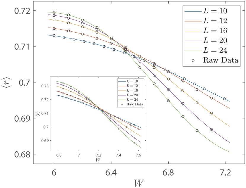
Figure 1: Level spacing ratio $\langle r\rangle$ as a function of the disorder strength $W$ for the class AI^† model. The circles are for raw data of $\langle r\rangle$, where an error is smaller than the circle size. The curves are from the polynomial fitting results with $m_{1},n_{1},m_{2},n_{2}$=(3, 3, 0, 1). Inset: the same plot for class A.

Numerical result and polynomial fitting— In order to obtain large number of eigenvalues for the level statistics and also guarantee that their eigenstates share almost similar critical disorder, we choose the energy window to be $10\%$ eigenvalues around $E=0$ in the complex Euler plane. $M$ is chosen in such a way that the total number of the eigenvalues reaches $5\times 10^{7}$ ($L<24$) and $10^{7}$ ($L=24$) for the class AI^†, and $10^{7}$ for the class A sup . Fig. 1 shows a plot of $\langle r\rangle$ as a function of disorder strength with the various system sizes. The plots for both class AI^† and class A models show critical points $W_{c}$, where the scale-invariant quantity $\langle r\rangle$ does not change with the system size $L$. We note that $W_{c}$ in the class A model is larger than that in the class AI^† model even though the former contains more randomness in the transfer. This is similar to the AT in Hermitian systems, and indicates that the AT in NH systems is also caused by quantum interference.

For localized phase ($W>W_{c}$), different energy levels have less correlations because of exponentially small overlap between eigenfunctions. In the thermodynamic limit, the nearest neighbor and next nearest neighbor levels become independent, and $z_{i}$ is equally distributed within a circle with radius one in the complex Euler plane. $\langle r\rangle_{\rm insulator}=\int_{0}^{1}r\rho(r)dr=2/3$ with $\rho(r)=2r$ the density of $r$ in the complex plane. We confirmed $\langle r\rangle\approx 0.66$ for strong disorder for both symmetry classes sup . On the other hand, the energy levels are correlated in delocalized phase ($W<W_{c}$) because of a spatial overlap between eigenfunctions. The overlap causes an level repulsion between the energy levels, which generally makes $\rho(r)$ near $r=0$ to be smaller in the delocalized phase than in the localized phase. Thus, $\langle r\rangle_{\rm metal}$ tends to be larger than $\langle r\rangle_{\rm insulator}$. We observed that $\langle r\rangle$ reaches a constant value in the metal phase in both models, where the constant value increases with the system size sup . In the thermodynamic limit, $\langle r\rangle$ in the metal phase reaches a certain universal value. This is analogous to metal phases of Hermitian systems in the three Wigner-Dyson (WD) classes Atas et al. (2013). Our calculation with the largest system size shows $\langle r\rangle_{\rm metal}\approx 0.720$ for the class AI^† model and $\langle r\rangle_{\rm metal}\approx 0.736$ for the class A model sup . The different values of $\langle r\rangle_{\rm metal}$ in the thermodynamic limit indicates that the two models belong to the different classes.

The LSR $\langle r\rangle$ takes a size-independent universal value at the critical point $W=W_{c}$ (TABLE 2). The critical LSR as well as the CE are evaluated in terms of the polynomial fitting method Slevin and Ohtsuki (2014). The criticality in each model is controlled by a saddle-point fixed point of a renormalization group equation for a certain effective theory, which describes the AT of the model. A standard scaling argument around the saddle-point fixed point gives $\langle r\rangle$ near the critical point by a universal function $\langle r\rangle=F(\phi_{1},\phi_{2})$. Thereby, $\phi_{1}\equiv u_{1}(w)L^{1/\nu}$ and $\phi_{2}\equiv u_{2}(w)L^{-y}$ stand for a relevant and the least irrelevant scaling variable around the postulated saddle-point fixed point; $1/\nu\!\ (>0)$ and $-y\!\ (<0)$ are the scaling dimensions of the relevant and the irrelevant scaling variables around the fixed point. $w$ is a normalized distance from the critical point; $w\equiv(W-W_{c})/W_{c}$. When $W$ is close enough to the critical disorder strength $W_{c}$, $u_{1}(w)$ and $u_{2}(w)$ can be Taylor expanded in small $w$. By definition, the expansions take forms of $u_{i}(w)\equiv\sum^{m_{i}}_{j=0}b_{i,j}w^{j}$ with $i=1,2$, $b_{1,0}=0$ and $b_{2,0}\neq 0$. For smaller $w$ and larger $L$, the universal function can be further expanded in small $\phi_{1}$ and $\phi_{2}$ as $F=\sum^{n_{1}}_{j_{1}=0}\sum^{n_{2}}_{j_{2}=0}a_{j_{1},j_{2}}\phi^{j_{1}}_{1}\phi^{j_{2}}_{2}$. For a given set of $(n_{1},n_{2},m_{1},m_{2})$, $\chi^{2}\equiv\sum^{N_{D}}_{k=1}(F_{k}-\langle r\rangle_{k})^{2}/\sigma^{2}_{\langle r\rangle_{k}}$ is minimized in terms of $W_{c}$, $\nu$, $-y$, $a_{i,j}$ and $b_{i,j}$ ($a_{1,0}=a_{0,1}=1$). Here each data point $k$ ($k=1,\cdots,N_{D}$) is specified by $L$ and $W$. $\langle r\rangle_{k}$ and $\sigma_{\langle r\rangle_{k}}$ are the mean value and the standard deviation at $k=(L,W)$, respectively, while $F_{k}$ is a fitting value from the polynomial expansion of $F$ at $k=(L,W)$. Fittings are carried out for several different $(n_{1},n_{2},m_{1},m_{2})$. Table 2 shows the fitting results with goodness of fit greater than 0.1. The 95$\%$ confidence intervals are determined by 1000 sets of $N_{D}$ number of synthetic data that are generated from the mean value and the standard deviation. $W_{c}$, $\nu$, $y$ and $\langle r\rangle_{c}$ are shown to be robust against the change of the expansion order and various system size and disorder range. We also confirm that our estimation is stable against changing the size of the energy windows sup .

The CE $\nu$ of the AT is evaluated as $\nu=0.99\pm 0.05$ for the 3D class AI^† and $\nu=1.09\pm 0.05$ for the 3D class A model, which are clearly distinct from $\nu=1.57\pm 0.01$ for the 3D orthogonal class Slevin and Ohtsuki (2018), and $\nu=1.44\pm 0.01$ for the 3D unitary class Slevin and Ohtsuki (1997, 2016) respectively. This unambiguously concludes that the AT in 3D class AI^† as well as 3D class A belongs to a new universality class that is different from any of the WD universality classes and in this respect, our result has confirmed that the non-Hermiticity changes the universality classes of the AT. It is also intriguing to see whether the AT in the 3D class AI^† and that in the 3D class A belong to the same universality class or not. However, our estimation of $\nu$ and $\langle r\rangle_{c}$ are quite close to each other within the 95$\%$ confidence intervals and it is hard to give a definite answer to this question. To answer this important question, we study in the following the spectral rigidity, level spacing distribution, and LSR distribution at the critical points of the two models.

Spectral rigidity— The spectral rigidity is defined by number variance $\Sigma_{2}\equiv\langle\delta N^{2}\rangle=\langle(N-\langle N\rangle)^{2}\rangle$, where $N$ is the number of eigenvalues in a fixed energy window and $\langle N\rangle$ stands for $N$ averaged over different disorder realizations. The spectral compressibility $\chi$ can be extracted by $\chi\equiv\lim_{L\rightarrow\infty}\lim_{N\rightarrow\infty}\frac{d\Sigma_{2}(N)}{d\langle N\rangle}$. Energy levels in insulator phase have less correlations and they show $\Sigma_{2}=\langle N\rangle$ in the thermodynamic limit. In metal phase, energy levels show the repulsive correlation, where $\Sigma_{2}\sim\ln(\langle N\rangle)$ and $\chi$ goes to the zero in the large $N$ limit.

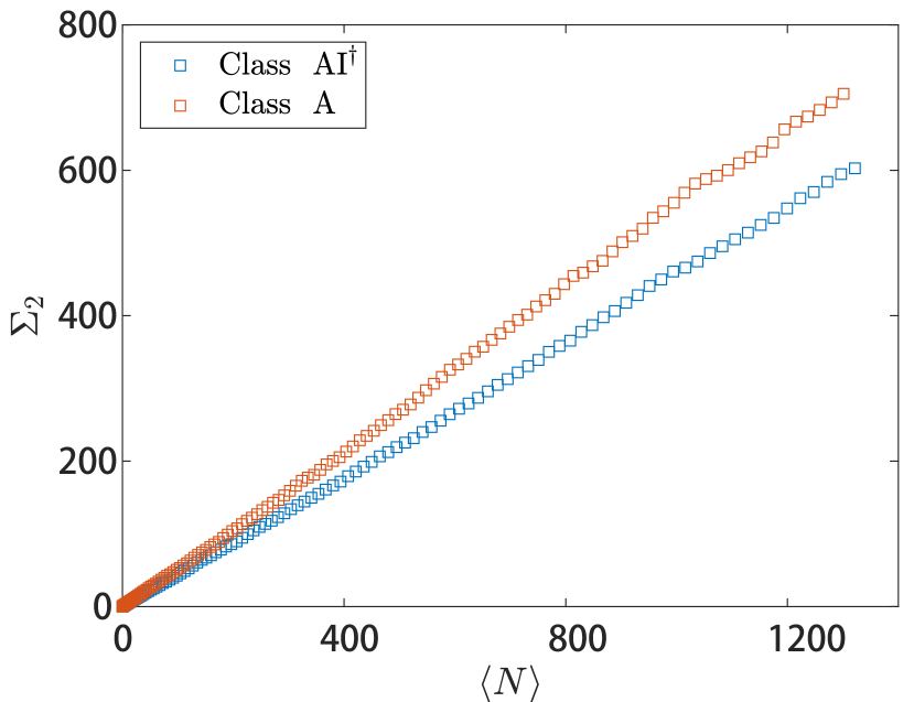
Figure 2: Number variance $\Sigma_{2}$ as a function of averaged level number $\langle N\rangle$ at the critical point ($W=6.3$ for class AI^† and $W=7.16$ for class A), and $\Sigma_{2}=\chi\langle N\rangle$ with $\chi\approx 0.46$ for class AI^† and $\chi\approx 0.55$ for class A. The plot comes from $10^{4}$ samples for class AI^† and 6400 samples for class A with $L=24$. Variable $\langle N\rangle$ is obtained by changing the energy window within the $10\%$ eigenvalues around $E=0$. The linear relationship holds true for the system size $L\geq 8$ with a consistent $\chi$ sup .

At the critical point, $\chi$ takes a universal value and it has been conjectured that $\chi$ is related with multifractal dimensions $D_{q}$ Rodriguez et al. (2011) as $2\chi+D_{2}/d=1$ Chalker et al. (1996a, b, c) and $\chi+D_{1}/d=1$ Bogomolny and Giraud (2011). Fig. 2 shows that $\Sigma_{2}$ at the critical point for the both NH systems is indeed linear in $\langle N\rangle$ in the the large $N$ limit. $\chi$ is extracted by a linear fitting, as $\chi\approx 0.46$ for the class AI^† case Huang and Shklovskii (2020b), and $\chi\approx 0.55$ for the class A case. These two values are clearly different from each other, and they are also distinct from the Hermitian cases; $\chi\approx 0.28$ for 3D orthogonal class Braun et al. (1998); Ndawana et al. (2002); Bogomolny and Giraud (2011); Ghosh et al. (2017); sup , and $\chi\approx 0.31$ for 3D unitary class sup .

Level spacing distribution— A level spacing distribution $P(s)$ plays an essential role in characterizing the AT in the Hermitian systems. $P(s)$ in metal phase can be described by the WD surmise Wigner (1951); Dyson (1962a, b) in random matrix theory, $P(s)=a_{\beta}s^{\beta}e^{-b_{\beta}s^{2}}$, where the Dyson index $\beta=1,2,4$ for orthogonal, unitary, and symplectic class, respectively. At the critical point, $P(s)\propto s^{\beta_{c}}$ for small $s$ region, where $\beta_{c}$ for each of the three classes are almost the same as the respective Dyson index $\beta$ in the metal phase Zharekeshev and Kramer (1995); Kawarabayashi et al. (1996). For larger $s$ region, $P(s)\propto e^{-\alpha s}$ with almost an identical value of $\alpha$ for these three WD symmetry classes; $\alpha=1.8\pm 0.1$ sup ; Batsch et al. (1996); Hofstetter (1996); Zharekeshev and Kramer (1995).

For the NH systems, things become more interesting. Our numerical results of $P(s)$ in insulator phase shows a 2D Poisson distribution Grobe et al. (1988), $P_{P}^{2D}(s)=\frac{\pi}{2}se^{-\pi s^{2}/4}$ for both classes sup . In metal phase, $P(s)$ for class A case sup follows the statistics of Ginibre ensembleGinibre (1965) with cubic repulsion ($\beta=3$) for small $s$ Grobe et al. (1988); Grobe and Haake (1989); Akemann et al. (2019), but not for the class AI^† case sup . This implies that the two classes belong to different symmetry classes according to level spacing distribution Hamazaki et al. (2020). At the critical point, the same asymptotic behaviors of $P(s)$ at small and large $s$ regions as in the Hermitian case hold true for the NH case with different values of $\alpha$ and $\beta_{c}$ (Fig. 3). Our numerical result shows that $\alpha=5.0\pm 0.1$ for class AI^†, $\alpha=4.5\pm 0.1$ for class A sup , which are larger than those for the three WD classes sup ; Batsch et al. (1996); Hofstetter (1996); Zharekeshev and Kramer (1995). We also find $\beta_{c}=2.6\pm 0.05$ for class AI^† and $\beta_{c}=2.9\pm 0.05$ for class A, which are also different from $\beta\approx 1$ for 3D orthogonal class and $\beta\approx 2$ for 3D unitary class, respectively sup .

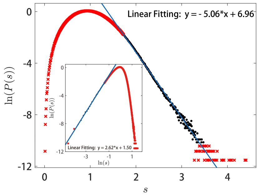
Figure 3: Critical level spacing distribution $P(s)$ at large $s$ and small $s$ (inset) for class AI^† at $W_{c}=6.3$. The small-$s$ behavior of $P(s)$ is fitted by $P(s)\propto s^{\beta_{c}}$ with $\beta_{c}\approx 2.62$ (blue solid line in the inset), and the large-$s$ behavior of $P(s)$ is fitted by $P(s)\propto e^{-\alpha s}$ with $\alpha\approx 5.06$ (blue solid line). The distribution is obtained from $10\%$ eigenvalues around $E=0$ of $10^{4}$ disorder realizations with $L=24$. Red crosses are data excluded from the linear fitting. Similar critical behaviors but with different $\beta_{c}$ and $\alpha$ are also observed for class A sup .

level spacing ratio distribution— The complex ratio $z_{i}$ contains information of its modulus $r_{i}\equiv|z_{i}|$ and angle $\theta_{i}\equiv{\rm arg}(z_{i})$. In insulator phase, $z_{i}$ is equally distributed in the complex plane due to the absence of the energy level correlation; $P(r)=2r$, and $P(\theta)=\frac{1}{2\pi}$ for both of the classes sup . In metal phase, $P(r)$ and $P(\theta)$ for the class A case is consistent with that for the Ginibre ensemble, but not for the class AI^† sup . The behaviors of $P(r)$ and $P(\theta)$ here are similar to $P(s)$, and all the three distributions exhibit the unique universal features in the metal phases of the AI^† and A classes. At the critical point, both $P(r)$ and $P(\theta)$ are independent of the system sizes for both classes sup , except for $P(\theta)$ with small deviation at two edges caused by the boundary effect Sá et al. (2020). We found it hard to distinguish the universality class of the AT in the class AI^† and that in the class A by the critical distributions of $P(r)$ and $P(\theta)$.

Summary— The Anderson transition driven by non-Hermitian disorder is studied by level statistics for 3D class AI^† and class A models. Critical exponents $\nu$ are estimated from the LSR by the polynomial fitting method and the estimated values conclude that the AT in these NH systems belong to new universality classes. Our estimation of $\nu$ for class AI^† is at variance with the preceding study Huang and Shklovskii (2020a), and we believe the discrepancy comes from the insufficient accuracy. Critical spectral compressibility is evaluated as $\chi\approx 0.46$ for class AI^† and $\chi\approx 0.55$ for class A, which are larger than those for 3D orthogonal and unitary classes. How the multifractal dimensions for the NH systems are related to the spectral compressibility at the critical point is an interesting open problem left for the future. The critical behavior of $P(s)$ at small and large $s$ regions in the NH systems are characterized by exponents $\beta_{c}$ and $\alpha$ as in the Hermitian case. Our numerical result for $\beta_{c}$ and $\alpha$ in the class AI^† and A are clearly distinct from each other and they are larger than those for 3D orthogonal and unitary classes. $P(s)$, $P(r)$ and $P(\theta)$ of class A in the metal phase are consistent with the statistics of the Ginibre ensemble, but those of the class AI^† are not. All the estimated critical values of $\nu$, $\chi$, $\beta_{c}$ and $\alpha$ conclude that the non-Hermiticity changes the universality class of the AT for 3D class AI^† and 3D class A.

Acknowledgment— X. L. thanks fruitful discussions with Dr. Yi Huang. X. L. was supported by National Natural Science Foundation of China of Grant No.51701190. T. O. was supported by JSPS KAKENHI Grants No. 16H06345 and 19H00658. R. S. was supported by the National Basic Research Programs of China (No. 2019YFA0308401) and by National Natural Science Foundation of China (No.11674011 and No. 12074008).

I supplemental materials

I.1 Polynomial fitting for non-Hermitian Anderson model and U(1) model

We study the tight-binding model on a three-dimensional cubic lattice (Anderson model, AM),

$${\cal H}=\sum_{i}\varepsilon_{i}c^{\dagger}_{i}c_{i}+\sum_{\langle i,j\rangle}V_{i,j}c^{\dagger}_{i}c_{j}$$ (2)

and U(1) model,

$${\cal H}=\sum_{i}\varepsilon_{i}c_{i}^{\dagger}c_{i}+\sum_{\langle i,j\rangle}e^{2\pi i\cdot\theta_{i,j}}V_{i,j}c_{i}^{\dagger}c_{j}$$ (3)

where $c_{i}^{\dagger}$ ($c_{i}$) is the creation (annihilation) operator for electrons at site $i$ and $\varepsilon_{i}$ is random onsite potential. $\langle i,j\rangle$ means that $i$ and $j$ are the nearest neighbor lattice sites to each other, $V_{i,j}=V_{j,i}=1$ are the nearest neighbor hopping term, and $\theta_{i,j}=-\theta_{j,i}$ is the random phase that distributes uniformly within $[0,1)$. To study the Anderson transition (AT) in the non-Hermitian (NH) system, we set $\varepsilon_{j}=w_{j}^{r}+iw_{j}^{i}$ with the imaginary unit $i$. $w_{j}^{r}$ and $w_{j}^{i}$ are independent random numbers, both of which distribute uniformly within $[-W/2,W/2]$ for a given disorder strength $W$.

Table 2: Polynomial fitting results for (a) Anderson model and (b) U(1) model with non-Hermitian (NH) disorders. The goodness of fit (GOF), critical disorder $W_{c}$, critical exponent $\nu$, the scaling dimension of the least irrelevant scaling variable $-y$, and critical level spacing ratio $\langle r\rangle_{c}$ are shown for different orders of the Taylor expansion of the scaling function $(m_{1},n_{1},m_{2},n_{2})$, for different system size range, and for different disorder range. The square bracket stands for the 95% confidence interval for each fitting result. Polynomial fittings with various energy windows (‘percent’), expansion orders, system size range, and disorder range have been carried out, for the purpose of proving the stability of the fitting results against these changes.

(a)NH Anderson model
percent	$L$	$W$	$m_{1}$	$n_{1}$	$m_{2}$	$n_{2}$	GOF	$W_{c}$	$\nu$	$y$	$\langle r\rangle_{c}$
10%	8-24	[6, 7.12]	3	3	0	1	0.11	6.28[6.26, 6.30]	1.046[1.012, 1.086]	1.75[1.65, 1.84]	0.7169[0.7163, 0.7177]
10%	10-24	[6, 7.19]	3	3	0	1	0.15	6.32[6.30, 6.34]	0.990[0.945, 1.040]	2.10[1.87, 2.35]	0.7155[0.7146, 0.7164]
10%	12-24	[5.9, 7.2]	3	3	0	1	0.13	6.34[6.32, 6.36]	0.942[0.897, 0.989]	2.53[2.14, 2.90]	0.7145[0.7138, 0.7154]
5%	8-24	[6.14, 7.3]	3	3	0	1	0.21	6.38[6.35, 6.40]	0.977[0.938, 1.022]	1.82[1.73, 1.90]	0.7157[0.7149, 0.7165]
5%	10-24	[6.14, 7.26]	3	3	0	1	0.17	6.37[6.33, 6.41]	0.948[0.878, 1.039]	1.77[1.54, 2.02]	0.7159[0.7143, 0.7179]
5%	12-24	[5.9, 7.3]	3	3	0	1	0.12	6.42[6.39, 6.45]	0.825[0.765, 0.893]	2.27[1.89, 2.60]	0.7134[0.7124, 0.7151]
(b)NH U(1) model
percent	$L$	$W$	$m_{1}$	$n_{1}$	$m_{2}$	$n_{2}$	GOF	$W_{c}$	$\nu$	$y$	$\langle r\rangle_{c}$
10%	8-24	[7, 7.56]	1	3	0	1	0.32	7.14[7.13, 7.15]	1.065[1.036, 1.100]	2.60[2.31, 2.89]	0.7178[0.7171, 0.7188]
10%	8-24	[7, 7.56]	2	3	0	1	0.43	7.15[7.14, 7.16]	1.068[1.034, 1.105]	2.63[2.35, 2.92]	0.7177[0.7169, 0.7186]
10%	8-24	[7, 7.56]	3	3	0	1	0.49	7.15[7.14, 7.16]	1.065[1.031, 1.103]	2.64[2.35, 2.92]	0.7177[0.7169, 0.7186]
10%	10-24	[6.8, 7.6]	3	3	0	1	0.12	7.14[7.12, 7.16]	1.091[1.050, 1.151]	2.50[1.88, 3.16]	0.7187[0.7170, 0.7201]
10%	12-24	[6.68, 7.64]	3	3	0	1	0.46	7.13[7.06, 7.16]	1.133[1.065, 1.411]	2.29[0.83, 4.62]	0.7187[0.7166, 0.7281]
5%	8-24	[7, 7.8]	2	3	0	1	0.09	7.23[7.22, 7.24]	1.028[1.000, 1.059]	2.37[2.18, 2.57]	0.7165[0.7155, 0.7176]
5%	8-24	[7, 7.8]	3	3	0	1	0.18	7.23[7.22, 7.24]	1.012[0.979, 1.048]	2.35[2.15, 2.54]	0.7167[0.7155, 0.7178]
5%	10-24	[6.8, 8]	3	3	0	1	0.23	7.23[7.22, 7.25]	1.012[0.979, 1.047]	2.40[2.09, 2.73]	0.7164[0.7152, 0.7179]
5%	12-24	[6.8, 8]	3	3	0	1	0.23	7.24[7.22, 7.25]	1.027[0.974, 1.079]	2.68[2.09, 3.38]	0.7158[0.7143, 0.7177]

Level spacing ratio $r_{i}$ for each complex-valued eigenvalue $E_{i}$ as

$$r_{i}\equiv|z_{i}|,$$ (4)

with

$$z_{i}\equiv\frac{E_{i}-E_{\rm NN}}{E_{i}-E_{\rm NNN}},$$ (5)

where $E_{\rm NN}$ and $E_{\rm NNN}$ are the nearest neighbor and next nearest neighbor to $E_{i}$ in the complex Euler plane. $z_{i}$ is a complex number with modulus and angle. Here we focus on the modulus of $z_{i}$ first. $r_{i}$ will be averaged within an energy window (see below) and then averaged over $M$ realizations of disordered systems. This gives a precise value of $\langle r\rangle$ with a standard deviation $\sigma^{2}_{\langle r\rangle}=\frac{1}{M-1}(\langle r^{2}\rangle-\langle r\rangle^{2})$.

In order to have enough energy levels whose critical $W$ for the AT are sufficiently close to that for $E=0$, we take only $10\%$ eigenvalues near $E=0$ in the Euler plane as the energy window, and calculate them for each disorder realization. Here, the periodic boundary condition is imposed in the three directions for both of the two NH models. We prepare $M$ disorder realizations so that the total number of eigenvalues for the statistics ($M\ \times 10\%\times L^{3}$) reaches $5\times 10^{7}$ ($L<24$) or $10^{7}$ ($L=24$) for the NH AM and $10^{7}$ ($L\leq 24$) for the NH U(1) model; $M=10^{6}$, $5\times 10^{5}$, $3\times 10^{5}$, $1.2\times 10^{5},$ $6\times 10^{4}$, $10^{4}$ for $L=8,\!\ 10,\!\ 12,\!\ 16,\!\ 20,\!\ 24$ in the AM, and $M=2\times 10^{5}$, $10^{5}$, $6\times 10^{4}$, $2.5\times 10^{4}$, $1.2\times 10^{4}$, $6.4\times 10^{3}$ for $L=8,\!\ 10,\!\ 12,\!\ 16,\!\ 20,\!\ 24$ in the U(1) model.

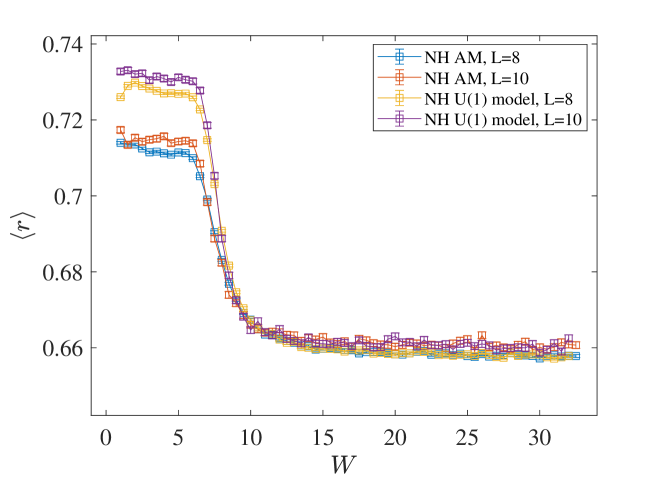
Figure 4: Averaged level spacing ratio $\langle r\rangle$ as a function of disorder. The level spacing ratio $r$ calculated from $10\%$ eigenvalues around $E=0$ is averaged over $M$ number of different disorder realizations. We take $M=10^{4}$, $10^{3}$ for the system size $L=8$, $10$, respectively, in non-Hermitian (NH) Anderson model (AM) and NH U(1) model. When $W$ is either very small or very large, $\langle r\rangle$ approaches constant values.

$\langle r\rangle$ goes to almost constant values when $W$ is far away from the critical point (FIG. 4). Consider first the very strong disorder region; $W\gg W_{c}$. In the thermodynamic limit, energy levels are distributed randomly without any correlations with others. Thus, $r$ could be any value within $0<r<1$ with equal probability. Hence

$$\langle r\rangle_{\rm insulator}=\int_{0}^{1}r\rho(r)dr=\frac{2}{3},$$ (6)

where the density for $r$ is determined from $\langle\rangle_{\rm insulator}=1$; $\rho(r)=2r$. Both models with the very strong disorder indeed show $\langle r\rangle\approx 0.66$ (FIG. 4).

Consider next the metal phase; $W\ll W_{c}$. The energy levels in the metal phase have repulsive interactions with others, because of spatial overlaps between the extended eigenfunctions. Accordingly, the density of $r$ near zero will be smaller than in the insulator phase, hence $\langle r\rangle_{\rm metal}>\langle r\rangle_{\rm insulator}$.

For the Hermitian case (Gaussian ensemble), a mean value of $r_{i}\equiv s_{i}/s_{i-1}$, where $s_{i}\equiv E_{i}-E_{i-1}$ on the real axis with $\{E_{i}\}$ ordered, takes a certain constant value in the metal phase. The value depends on the symmetry class in the three Wigner-Dyson (WD) classes Atas et al. (2013). For the non-Hermitian case, we found that $\langle r\rangle$ reaches a constant value in the weaker disorder region ($W\leq W_{c}$), and the value increases with the system size for both models (FIG. 4). For example, $\langle r\rangle=0.7182$, $0.7201$ for $L=12$, $20$ at $W=1$ for the NH AM and $\langle r\rangle=0.7307$, $0.7329$, $0.7353$, $0.7363$ for $L=10$, $12$, $16$, $20$ at $W=1$ for the NH U(1) model. By an extrapolation, we speculate $\langle r\rangle_{\rm metal}$ in the thermodynamic limit as $0.720$, and $0.736$ for the NH AM and U(1) models, respectively. Thus, the distributions of $r$ in the metal phases are different in the two NH models (FIG. 10).

In order to characterize the Anderson transition, the scale-invariant quantity $\langle r\rangle$ is adopted. We estimate the critical exponent (CE) $\nu$ by polynomial fitting method Slevin and Ohtsuki (2014), with various system size range, disorder range and expansion orders in the polynomial fitting. Moreover, we narrow the energy window from the $10\%$ eigenvalues around $E=0$ to $5\%$ to see the stability of the polynomial fitting results. The results are shown in TABLE 2 (a) for NH AM and (b) for NH U(1) model.

CEs are consistent with each other for data sets with various system size range, disorder range, and expansion orders. This implies that our results are stable and precise. Moreover, CEs estimated from the $5\%$ eigenvalues energy window are consistent with that from the $10\%$ eigenvalues energy window, although they have a tendency to become smaller. CEs estimated from the $10\%$ eigenvalues energy window is preferable because of the abundant energy levels. We conclude $\nu=0.99\pm 0.05$ for NH AM and $\nu=1.09\pm 0.05$ for NH U(1) model.

When the energy window is narrowed from 10% to 5% eigenvalues, the critical disorders in the both models tend to get larger; delocalized states at the band center are more robust against the disorder. Besides, the CE for the NH AM changes to smaller values, when the data points for the smaller system sizes are excluded. The change of the CE in the NH AM becomes more prominent with the 5% energy window than with the 10% energy window. This means that the CE for the NH AM suffers from a systematic error by the choice of the energy windows. For the NH U(1) model, on the one hand, CEs extracted from the 5% energy window stay nearly constant against the exclusion of the data from the smaller system sizes; the fitting of the NH U(1) model is much more stable than that of the NH AM.

The difference of the stability in the fittings between the two models could be explained as follows. In the limit of the strongly localized phase, the level spacing ratio reaches the same value for the both models; $\langle r\rangle=2/3$, while $\langle r\rangle$ in the limit of the delocalized phase goes to two different constant values in the two models respectively (FIG. 4); there are two plateau regimes of $\langle r\rangle$ as a function of the disorder strength in these models. Note that data points near the plateau regimes should not be included for the scaling analysis, for they are likely outside the critical regime. FIG. 1 in the main text shows that for the NH AM, the intersection of curves of $\langle r\rangle$ is quite close to the plateau value of $\langle r\rangle$ in the limit of the delocalized phase. Therefore, it is expected that a valid data range of the polynomial fitting in the NH AM becomes quite small in the side of the metal phase. On the other hand, the intersection for the NH U(1) model is relatively far away from the plateau value in the delocalized phase; the valid data range of the fitting becomes much wider in the NH U(1) model.

I.2 Spectral rigidity

The spectral rigidity is defined by a number variance within an energy window

$$\Sigma_{2}\equiv\langle\delta N^{2}\rangle=\langle(N-\langle N\rangle)^{2}\rangle,$$ (7)

where $N$ is the number of eigenvalues within the same energy window, and $\langle\cdots\rangle$ stands for the average over $M$ disorder realizations. $M$ is typically on the order of or larger than $10^{4}$. The spectral compressibility $\chi$ can be extracted by

$$\chi\equiv\lim_{L\rightarrow\infty}\lim_{N\rightarrow\infty}\frac{d\Sigma_{2}(N)}{d\langle N\rangle}.$$ (8)

Here, we set a circular energy window around $E=0$ as $\{|E|<E_{\rm bound}\}$ with $E_{\rm bound}>0$. To calculate the spectral compressibility, we decrease the energy window (reduce $E_{\rm bound}$) for a fixed (but sufficiently large) system size.

Let us focus on the spectral compressibility at a critical point for the AT; $W=W_{c}$. From TABLE 2, We choose $W_{c}=6.3$ for the NH AM and $W_{c}=7.16$ for the NH U(1) model. We prepare $M$ disorder realizations with $M=2\times 10^{5}$, $10^{5}$, $3\times 10^{5}$, $1.2\times 10^{5}$, $6\times 10^{4}$, $10^{4}$ for $L=8$, $10$, $12$, $16$, $20$, $24$ for the NH AM and $N=2\times 10^{5}$, $10^{5}$, $6\times 10^{4}$, $2.5\times 10^{4}$, $1.2\times 10^{4}$, $6.4\times 10^{3}$ for $L=8$, $10$, $12$, $16$, $20$, $24$ for the NH U(1) model. In order to extract $\chi$, we change the energy window, namely $E_{\rm bound}$, within $10\%$ eigenvalues for a fixed system size $L$, and obtain various $\langle N\rangle$ and $\Sigma_{2}$ for each system size $L$. Then we carry out the linear fitting for $\Sigma_{2}$ vs. $\langle N\rangle$ for each $L$ (TABLE 3). From TABLE 3, we found that $\chi$ thus obtained is stable against changing the system size $L$. We thus choose $\chi$ as of the largest system size in TABLE 3; $\chi\approx 0.46$ for the NH AM and $\chi\approx 0.55$ for the NH U(1) model.

For the 3D Hermitian AM, the critical spectral compressibility $\chi$ has been already studied by others Ndawana et al. (2002); Bogomolny and Giraud (2011); Ghosh et al. (2017). For the comparison with the NH cases, we recalculate the same quantity for the Hermitian case for much smaller size system ($L=10$). The 10$\%$ eigenvalues around $E=0$ are calculated at the critical disorder strength of the AT ($W=W_{c}$), and the average number and number variance are taken over $10^{5}$ disorder realizations for the AM ($W_{c}=16.5$, see Slevin and Ohtsuki (2018)), and over $6400$ disorder realizations for the U(1) model ($W_{c}=18.8$, see Slevin and Ohtsuki (2016)). We narrow the energy window, obtain the various $\langle N\rangle$ and $\Sigma_{2}$, and carry out the linear fitting for $\Sigma_{2}$ vs. $\langle N\rangle$. This gives $\chi\approx 0.28$ Bogomolny and Giraud (2011) for the Hermitian AM and $\chi\approx 0.31$ for the Hermitian U(1) model at the critical point of the AT.

Table 3: Linear fitting results of critical spectral compressibility $\chi$ of various system size $L$ for non-Hermitian (NH) Anderson model and U(1) model.

	8	10	12	16	20	24
NH Anderson model	0.4658	0.461	0.4593	0.4585	0.457	0.4592
NH U(1) model	0.5439	0.5425	0.5456	0.5469	0.5397	0.5533

I.3 Level spacing distribution for Gaussian random matrix

For the Hermitian case, the level spacing distribution $P(s)$ in a metal phase is well described by the Wigner-Dyson (WD) surmise Wigner (1951) in random matrix theory;

$$P_{\rm GOE}(s) =\frac{\pi}{2}se^{-\frac{\pi}{4}s^{2}},\ \ \beta=1$$

$$P_{\rm GUE}(s) =\frac{32}{\pi^{2}}s^{2}e^{-\frac{4}{\pi}s^{2}},\ \ \beta=2$$

$$P_{\rm GSE}(s) =\frac{2^{18}}{3^{6}\pi^{3}}s^{4}e^{-\frac{64}{9\pi}s^{2}},\ \ \beta=4$$ (9)

where $\beta$ is the power exponent for smaller $s$ region (the Dyson index), and $\beta=1,2,4$ for Gaussian Orthogonal ensemble (GOE),Gaussian Unitary ensemble (GUE), and Gaussian Symplectic ensemble (GSE), respectively. $P(s)\propto s^{\beta}$ for the smaller $s$ region is caused by repulsive interactions between the energy levels in the metal phase.

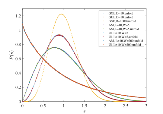
Figure 5: Level spacing distribution $P(s)$ for the Hermitian case. $W=5,200$ for Hermitian Anderson model (AM), and $W=2,200$ for U(1) models, corresponding to metal and insulator phase ($W_{c}=16.5$ for the AM, and $W_{c}=18.8$ for the U(1) model). The $10\%$ eigenvalues around $E=0$ are calculated over $10^{5}$ samples for Hermitian AM and U(1) models ($L=10$). All the eigenvalues of the random matrix are calculated over $6\times 10^{6}$ samples with the matrix dimension $D=10$ for the GOE, GUE, and over $64000$ samples with the matrix dimension $D=1000$ for GSE. $P(s)$ with $s$ that is not unfolded are also tried for comparison and unfolding makes no difference here, because density of states is almost constant in the region calculated.

In insulator phase, $P(s)$ obeys the Poisson distribution,

$$P(s)=e^{-s},$$ (10)

since energy levels are uncorrelated with others. At the critical point of the AT,

$$P(s)\propto s^{\beta_{c}},$$ (11)

for smaller $s$ region and

$$P(s)\propto e^{-\alpha s},$$ (12)

for larger $s$ region.

For the purpose of the comparison, we recalculated the level spacing distribution $P(s)$ of the Hermitian WD random matrix. We prepare the Hermitian random matrix $H$ as,

$$H=(A+A^{\dagger})/2,$$ (13)

where $A$ is a random matrix with a restriction according to the symmetry. For GOE, $H^{*}=H$, so $A$ is a real random matrix. For GUE, there is no restriction for $H$, so that $A$ is a complex random matrix. For GSE, $\Sigma_{y}H^{*}\Sigma_{y}=H$, with

$$\Sigma_{y}=\begin{pmatrix}0&-i\\ i&0\\ \end{pmatrix},$$ (14)

so that $A$ has the following structure,

$$A=\begin{pmatrix}X&Y\\ -Y^{*}&X^{*}\\ \end{pmatrix},$$ (15)

where $X$, $Y$ are complex random matrices. Each element of the real random matrix is produced by the same Gaussian distribution, and is independent. Real and imaginary parts of each element of the complex random matrix are produced by the same Gaussian distribution, and are independent. Eigenvalues in the GSE are doubly degenerate by the symmetry. We excluded this trivial degeneracy in the energy level statistics of $P(s)$.We calculate all the eigenvalues of the random matrix with the matrix dimension $D=10$ and take energy level statistics over $6\times 10^{6}$ different realizations of the random matrix for GOE and GUE, while energy level statistics of the random matrix with the matrix dimension $D=1000$ is taken over $64000$ different realizations of the random matrix for GSE. For the unfolded energy levels in FIG. 5, we first calculate an averaged density of state out of many samples. In terms of the averaged density of states $\rho(E)$, we map an energy level in each sample into an integrated density of states (IDOS);

$${\rm IDOS}(E_{i})=\int^{E_{i}}\rho(E)dE.$$ (16)

The level spacing corrected by the averaged density of states, $s_{i}$, is given by a difference between the neighboring IDOSs,

$$s_{i}\equiv{\rm IDOS}(E_{i+1})-{\rm IDOS}(E_{i}).$$ (17)

Our recalculation in FIG. 5 reproduces the Dyson index; $\beta\approx 1$ for GOE, $\beta\approx 2$ for GUE, $\beta\approx 4$ for GSE.

I.4 Level spacing distribution for Anderson model and U(1) model with Hermitian disorder

For comparison, we also (re)calculate the level spacing distribution for Hermitian AM [Eq. (2)] and U(1) models [Eq. (3)] with real random onsite potentials. We calculate $10\%$ of the whole eigenvalues near $E=0$ with the system size $L=10$ for every disorder realization, and take the statistics over $10^{5}$ different disorder realizations. FIG. 5 shows that $P(s)$ in metal phase thus obtained for AM and U(1) model are consistent with $P(s)$ for GOE and GUE, respectively. Moreover, $P(s)$ with and without unfolding are almost identical to each other in metal phase. $P(s)$ with and without unfolding are so close to each other, because the density of states within the $10\%$ energy windows is nearly constant in energy in metal phase. The unfolding process produces an error in $P(s)$ for small $s$ region, breaking a linear relationship; $\ln P(s)\propto\ln s$. We do not use the unfolding process when focusing on the behaviors of $P(s)$ at small-$s$ region.

At the critical point, $P(s)\propto s^{\beta_{c}}$ for small $s$ region, where critical power-law exponent $\beta_{c}$ takes almost the same exponent as the corresponding Dyson index $\beta$ for every WD classes; $\beta_{c}\approx\beta$ Kawarabayashi et al. (1996). $P(s)\propto e^{-\alpha s}$ for large $s$ region, where $\alpha$ takes almost the same value for the three WD classes; $\alpha=1.8\pm 0.1$ Batsch et al. (1996); Hofstetter (1996); Zharekeshev and Kramer (1995). In our calculation (FIG. 6), $\beta_{c}\approx 0.98$, and $\alpha\approx 1.79$ at the critical point of the Hermitian AM ($W_{c}=16.5$), and $\beta_{c}\approx 2.01$ and $\alpha\approx 1.71$ at critical point of the Hermitian U(1) model ($W_{c}=18.8$).

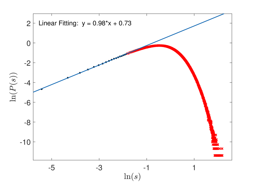
(a) Hermitian Anderson model, $W_{c}$=16.5; $\beta_{c}\approx 0.98$

(b) Hermitian U(1) model, at $W_{c}$=18.8; $\beta_{c}\approx 2.01$

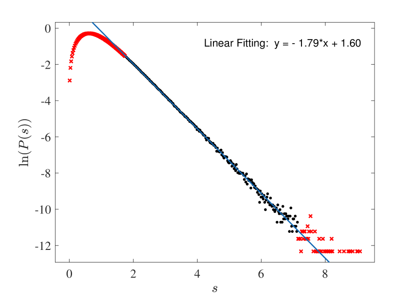
(c) Hermitian Anderson model, at $W_{c}$=16.5; $\alpha\approx 1.79$

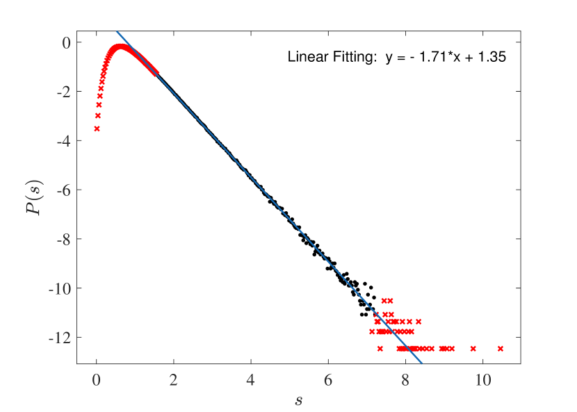
(d) Hermitian U(1) model, $W_{c}$=18.8; $\alpha\approx 1.71$

Figure 6: Level spacing distribution $P(s)$ for small $s$ ((a), (b); without unfolding), and for large $s$ ((c), (d); with unfolding). The data comes from $10^{5}$ disorder realizations with $L=10$ for both models. The data are fitted by $P(s)\propto s^{\beta_{c}}$ at small s and $P(s)\propto e^{-\alpha s}$ at large s. Red points are data excluded for the linear fitting.

I.5 Level spacing distribution for Ginibre ensemble

Ginibre ensembles are classes of ensembles for non-Hermitian random matrices Ginibre (1965), and therefore they might be useful for understanding the energy level statistics and the AT in a non-Hermitian disorder system. According to the classification, there exist three kinds of the Ginibre ensembles; Ginibre Orthogonal ensemble (GinOE) ($H^{*}=H$), Ginibre Unitary ensemble (GinUE) (no restriction on $H$), and Ginibre Symplectic ensemble (GinSE) ($\Sigma_{y}H^{*}\Sigma_{y}=H$). The matrix $A$ for GOE, GUE, and GSE without Eq. (13) corresponds to random matrix in GinOE, GinUE, and GinSE, respectively. GinOE, GinUE, GinSE correspond to the symmetry class AI, A, AII in the classification for the NH system. Because of the symmetry, eigenvalues in GinOE and GinSE come in pairs; $\{E_{i},E_{i}^{*}\}$, and eigenvalues in the upper-half Euler plane are sufficient for the energy level statistics. The double degeneracy on the real axis needs to be excluded. We thus use only those eigenvalues whose imaginary parts are greater than 1, to determine the energy level statistics. Now the eigenvalues are complex number and the level spacing $s$ is defined by

$$s_{i}=|E_{i}-E_{\rm NN}|$$ (18)

where $E_{\rm NN}$ is the nearest neighbor for $E_{i}$. Here the density of states in complex Euler plane is almost constant in the region calculated, so that we omit the unfolding process. For small $s$, $P(s)$ of all these three kinds of the random matrix, GinOE, GinUE, and GinSE, obeys the same distribution (FIG. 7(b)) with a cubic repulsion; $P(s)\propto s^{3}$ Hamazaki et al. (2020).

I.6 Level spacing distribution for Anderson model and U(1) model with non-Hermitian disorder

Level spacing distribution are calculated for the NH AM (Eq. 2) and U(1) models (Eq. 3). In insulator, $P(s)$ takes the 2D Poisson distribution Grobe et al. (1988),

$$P_{P}^{2D}(s)=\frac{\pi}{2}se^{-\pi s^{2}/4}.$$ (19)

To test this formula, we calculates $10\%$ eigenvalues around $E=0$ in the complex Euler plane for the NH AM and U(1) model with $L=12$ at $W=100$, where the eigenstates in both models are in insulator phase. We determine $P(s)$ out of the $10\%$ eigenvalues calculated over $6\times 10^{4}$ different disorder realizations. $P(s)$ thus determined takes the same 2D Poisson distribution in the both models (FIG. 7(a)).

To calculate $P(s)$ in metal phase, we calculate the $10\%$ eigenvalues around $E=0$ for NH AM and U(1) model with $L=16$ at $W=3$, where it is guaranteed that all the eigenstates within the $10\%$ circular energy window are in the metal phase. We find that $P(s)$ for NH U(1) model is consistent with that for GinOE, GinUE, GinSE (FIG. 7(b)), but $P(s)$ for NH AM deviates from that for GinOE, GinUE, GinSE. In small $s$ region, $P(s)$ behaves as $s^{\beta}$, where $\beta\approx 2.74$ for NH AM and $\beta\approx 2.93$ for NH U(1) model (FIG. 8). This is consistent with ref. Hamazaki et al. (2020) where the class AI^† shows unique $P(s)$, different from $P(s)$ for the class A (FIG. 7(b)).

To calculate $P(s)$ at the critical point, we calculate the $10\%$ eigenvalues around $E=0$ for the NH AM and U(1) model at $W=W_{c}$ ($W_{c}\approx 6.3$ for NH AM and $W_{c}\approx 7.16$ for NH U(1) model). The system size $L$ and the number of disorder realizations $M$ are set as $M=2\times 10^{5}$, $10^{5}$, $3\times 10^{5}$, $1.2\times 10^{5}$, $6\times 10^{4}$, $10^{4}$ for $L=8$, $10$, $12$, $16$, $20$, $24$ for the NH AM, and $M=2\times 10^{5}$, $10^{5}$, $6\times 10^{4}$, $2.5\times 10^{4}$, $1.2\times 10^{4}$, $6.4\times 10^{3}$ for $L=8$, $10$, $12$, $16$, $20$, $24$ for the NH U(1) model. For each $L$, $P(s)$ is determined from the $10\%$ eigenvalues calculated over the $M$ different disorder realizations. We fit $P(s)$ thus obtained as $s^{\beta_{c}}$ for small $s$ and as $e^{-\alpha s}$ for large $s$. $\beta_{c}$ and $\alpha$ are estimated for each system size $L$ (FIG. 8 and TABLE 4). We find that the fitted values of $\beta_{c}$ and $\alpha$ are robust against the change of system size; $\beta_{c}=2.6\pm 0.05$ , $\alpha=5.0\pm 0.1$ for NH AM and $\beta_{c}=2.9\pm 0.05$ , $\alpha=4.5\pm 0.1$ for NH U(1) model.

Table 4: Linear fitting result of critical level spacing distribution $P(s)$ for small and large $s$ regions. The fitting by $e^{-\alpha s}$ for the large $s$ region gives $\alpha$ and the fitting by $s^{\beta_{c}}$ for the small $s$ region gives $\beta_{c}$.

Model		8	10	12	16	20	24
NH AM	$\alpha$	4.75	4.8	4.9	4.9	5.0	5.06
NH AM	$\beta_{c}$	2.61	2.6	2.63	2.6	2.56	2.62
NH U(1) model	$\alpha$	4.1	4.1	4.3	4.4	4.46	4.61
NH U(1) model	$\beta_{c}$	2.96	2.98	2.96	2.95	2.88	2.84

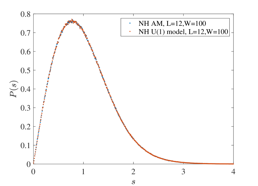
(a) $P(s)$ for insulator phase

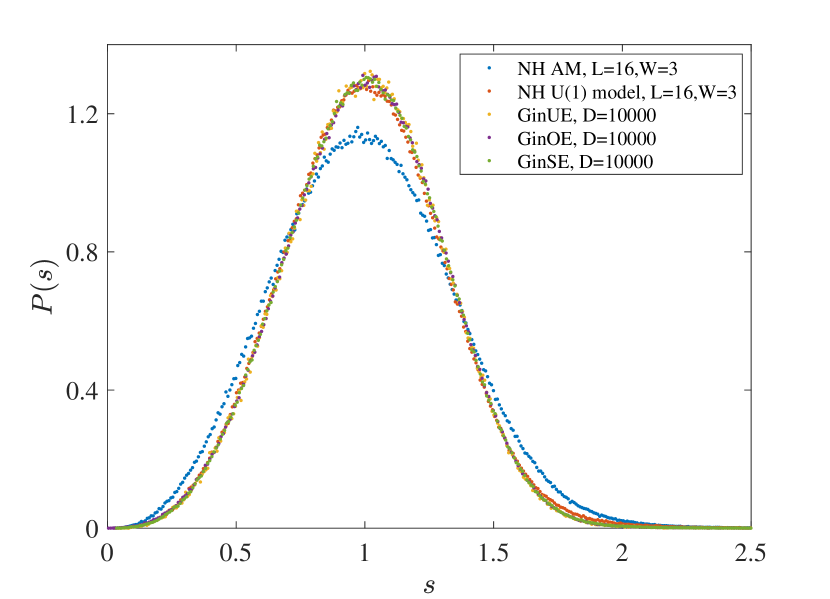
(b) $P(s)$ for metal phase and Ginibre ensembles

Figure 7: Level spacing distribution $P(s)$ in (a) insulator phase ($W=100$) and (b) metal phase ($W=3$) of non-Hermitian (NH) Anderson model (AM) and U(1) model. In (b)$P(s)$’s for GinUE, GinOE, GinSE with matrix dimension $D=10^{4}$ are also shown; 64 samples for GinUE and 640 samples for GinOE and GinSE. The distributions for insulator phase are constructed out of the $10\%$ eigenvalues around $E=0$ over $6\times 10^{4}$ samples for both models ($L=12$). The distributions for metal phase are calculated from $10\%$ eigenvalues around $E=0$ over $6400$ samples for both models ($L=16$).

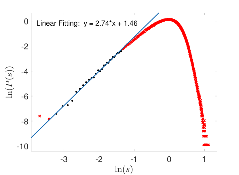
(a) NH Anderson model at $W=3$ (metal phase); $\beta\approx 2.74$

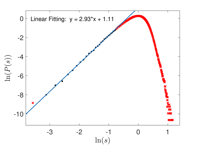
(b) NH U(1) model at $W=3$ (metal phase); $\beta\approx 2.93$

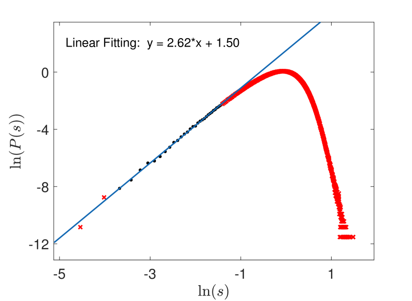
(c) NH Anderson model at $W_{c}=6.3$; $\beta_{c}\approx 2.62$

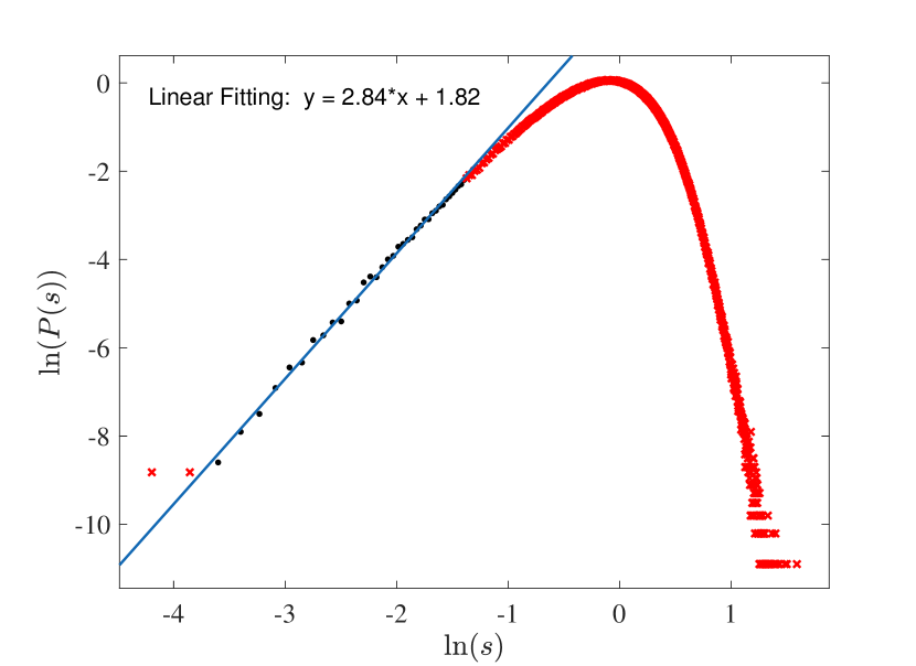
(d) NH U(1) model at $W_{c}=7.16$; $\beta_{c}\approx 2.84$

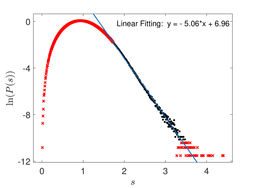
(e) NH Anderson model at $W_{c}=6.3$; $\alpha\approx 5.06$

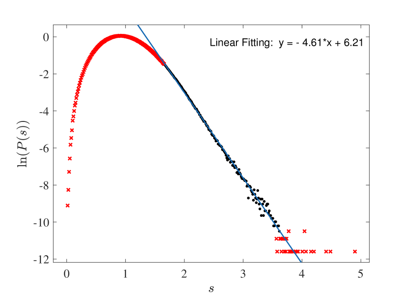
(f) NH U(1) model at $W_{c}=7.16$; $\alpha\approx 4.61$

Figure 8: Level spacing distribution $P(s)$ at small $s$ [(a)-(d)] and large $s$ [(e), (f)]. The blue lines are fitting curves by $P(s)\propto s^{\beta_{c}}$ at small $s$ and $P(s)\propto e^{-\alpha s}$ at large $s$. In metal phase [(a), (b); $W=3$], the data comes from $6400$ disorder realizations with $L=16$. At the critical point [(c)-(f); $W=W_{c}$], we take $W_{c}=6.3$, $L=24$ and $10^{4}$ samples for the non-Hermitian (NH) Anderson model, and $W_{c}=7.16$, $L=24$ and $6400$ samples for the NH U(1) model. Red points are data excluded for the linear fitting.

I.7 Level spacing ratio distribution for the Hermitian system

For the Hermitian case, we consider a distribution of level spacing ratio $r$, that is defined byOganesyan and Huse (2007)

$$r_{i}\equiv{\rm min}\Big{(}\frac{E_{i+1}-E_{i}}{E_{i}-E_{i-1}},\frac{E_{i}-E_{i-1}}{E_{i+1}-E_{i}}\Big{)}.$$ (20)

Here $\{E_{i}\}$ are ordered in the ascending order ($E_{1}<E_{2}<E_{3}\cdots$). For comparison, we calculate the level spacing ratio distribution, $P(r)$, for the random matrix in GOE, GUE and GSE and for the Hermitian AM, U(1) models (FIG. 9). A random matrix theory Atas et al. (2013) tells that $P(r)$ in the metal phase is given by

$$P(r)=\frac{1}{C_{\beta}}\frac{(r+r^{2})^{\beta}}{(1+r+r^{2})^{1+\frac{3}{2}\beta}}\Theta(1-r).$$ (21)

Here $C_{\beta}$ is a constant, $\beta=1,2,4$ for GOE, GUE, and GSE, respectively, and $\Theta(x)$ is the Heaviside step function.

In insulator, $P(r)$ is given by Atas et al. (2013)

$$P(r)=\frac{2}{(1+r)^{2}}\Theta(1-r).$$ (22)

for all the three WD classes. FIG. 9 shows that $P(r)$ in metal phase of the Hermitian AM and U(1) models are consistent with $P(r)$ of GOE and GUE, respectively. It also shows that $P(r)$ in the insulator phase has the same distribution as in Eq. (22) for both models.

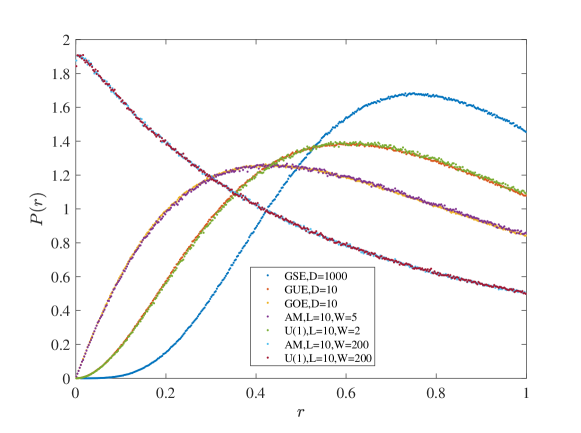
Figure 9: Level spacing ratio distribution $P(r)$ for GOE, GUE, GSE, the Hermitian Anderson model (AM) and U(1) model. We set the matrix dimension $D=10$ with $6\times 10^{6}$ realizations for GOE, GUE, and $D=1000$ with $64000$ realizations for GSE. For the Hermitian Anderson model and U(1) model, $P(r)$ is obtained from $10\%$ eigenvalues around $E=0$ calculated with the system size $L=10$ and $10^{5}$ samples.

I.8 Level spacing ratio distribution for non-Hermitian system

For the non-Hermitian case, we can consider not only the level spacing ratio $r$ but also the angle of $z_{i}$,

$$\theta_{i}\equiv{\arg}(z_{i}),$$ (23)

where $z_{i}$ is defined in Eq. (5). To see distributions of $r$ and $\theta$ in metal phase, we calculate $10\%$ eigenvalues around $E=0$ in the complex Euler plane for NH AM and U(1) model at $W=3$. We take the statistics over 6400 disorder realizations, to obtain the level spacing ratio distributions, $P(r)$ and $P(\theta)$. $P(r)$ and $P(\theta)$ in metal phase of the NH U(1) model are consistent with those of the GinUE. However, $P(r)$ and $P(\theta)$ in metal phase of the NH AM behave quite differently from the GinUE. This supports the conclusion of Ref. Hamazaki et al. (2020) that the metal phase of the NH AM and the metal phase in the NH U(1) model belong to two different universality classes. Noted that FIG. 10 also shows a small deviation between $P(\theta)$ of the NH U(1) model and $P(\theta)$ of the GinUE. We speculate that $\theta$ is more sensitive to the finite-system-size effect than $r$, because of boundary effects Sá et al. (2020).

FIG. 11 (a)-(d) show behaviors of $P(r)$ and $P(\theta)$ from metal phase to insulator phase in the NH AM and NH U(1) model. $P(r)$ becomes linear in $r$ in the insulator phase for both models. This observation is consistent with that in Ref. Sá et al. (2020). On the other hand, $P(\theta)$ shows a small peak at $\theta=0$ in the insulator phase for both models (FIG. 11 (e)). This observation is different from Ref. Sá et al. (2020). We speculate that the small peak in $P(\theta)$ come from the boundary effect, as pointed out in Ref Sá et al. (2020). Namely, those $E_{i}$ around the boundary of the $10\%$ circular energy window have higher chance to give smaller $\theta_{i}$, because such $E_{i}$ is apt to find its nearest ($E_{\rm NN}$) and next nearest neighbor ($E_{\rm NNN}$) in the same direction (an inner direction of the circular window; toward $E=0$). For calculations with the smaller system size, these eigenvalues near the circular boundary have considerable effect, causing a small peak at $\theta=0$ in $P(\theta)$. To uphold this speculation, we also calculate all the eigenvalues of the NH U(1) model with $L=20$ at $W=100$, and take the statistics over 640 samples. $P(\theta)$ thus obtained is flat in $\theta$ as expected (FIG. 11(f)).

FIG. 12 shows critical $P(r)$ and $P(\theta)$ for the two NH models. $P(\theta)$ shows some amount of size dependences as $|\theta|$ approaches $\pi$, where $P(\theta)$ for the large $\theta$ has a tendency to be larger for larger system size. In other words, $P(\theta)$ for the small $\theta$ tends to be smaller for the larger system. We speculate that this size dependence also partially comes from the boundary effect mentioned above. Note also that $P(r)$ and $P(\theta)$ are almost identical in the two models, except for small deviations observed in $P(r)$ at smaller $r$ (FIG. 12 (f)) and $P(\theta)$ at larger $\theta$ (FIG. 12 (e)). We conclude that it is hard to distinguish the two different universality classes in NH AM and NH U(1) models in terms of critical distributions of $P(r)$ and $P(\theta)$.

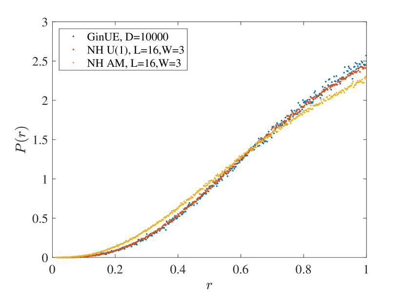
(a) $P(r)$

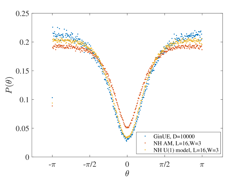
(b) $P(\theta)$

Figure 10: $P(r)$ and $P(\theta)$ for the Ginibre unitary ensemble, non-Hermitian (NH) Anderson model ($W=3$), NH U(1) model ($W=3$). We take 64 samples for the GinUE, $10\%$ eigenvalues around $E=0$ over 6400 samples for the NH Anderson model and U(1) model. It is guaranteed that the $10\%$ eigenvalues around $E=0$ in these two NH models are in the metal phase at $W=3$.

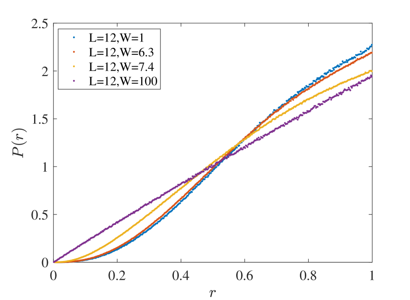
(a) $P(r)$ for NH AM in metal phase ($W=1$), critical point ($W=6.3$) and insulator phase ($W=7.4,100$)

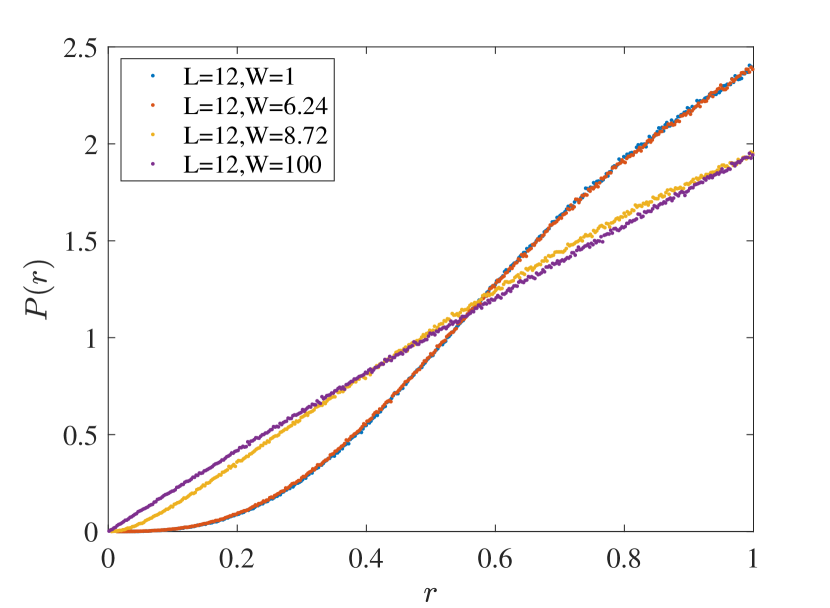
(b) $P(r)$ for NH U(1) model in metal phase ($W=1,6.24$) and insulator phase ($W=8.72,100$)

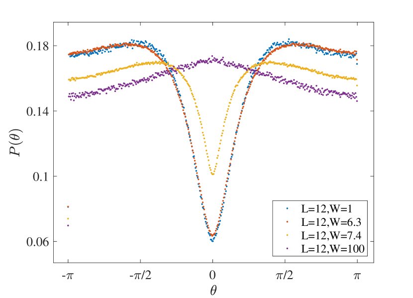
(c) $P(\theta)$ for NH AM

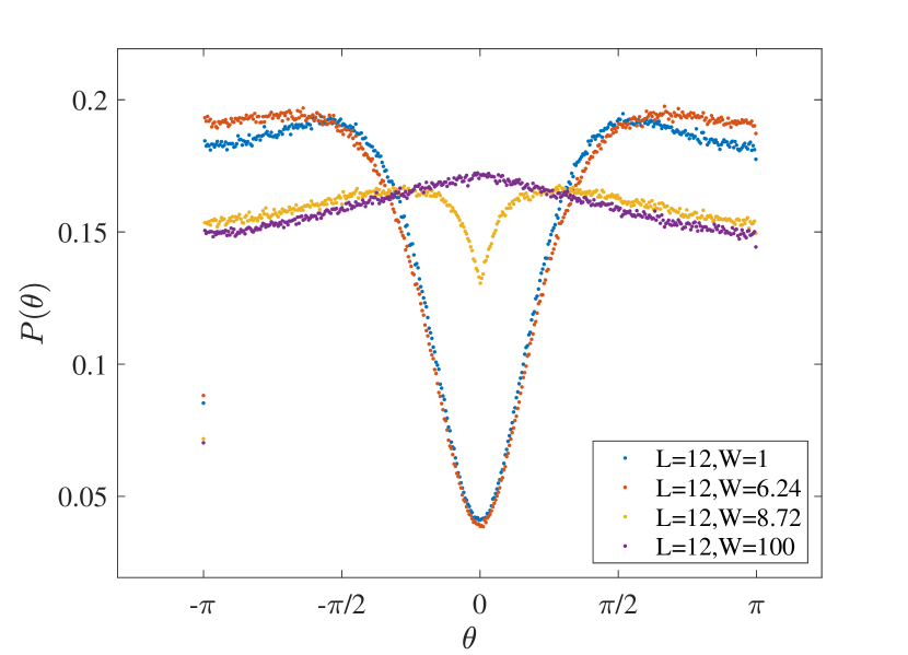
(d) $P(\theta)$ for NH U(1) model

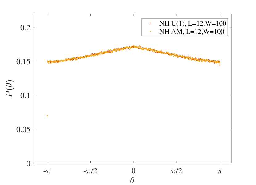
(e) $P(\theta)$ for NH AM and U(1) model

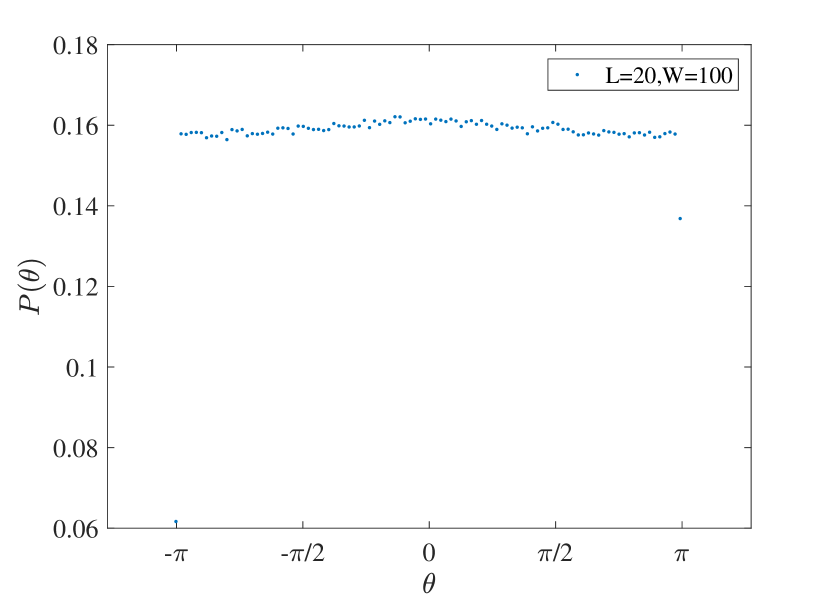
(f) $P(\theta)$ for NH U(1) model with $L=20$, $W=100$, $100\%$ eigenvalues.

Figure 11: $P(r)$ and $P(\theta)$ from metal to insulator phase (a)-(d), and (e) comparison of $P(\theta)$ between non-Hermitian (NH) Anderson model (AM) and U(1) model. We take $10\%$ eigenvalues around $E=0$ over $6\times 10^{4}$ samples (NH U(1) model), $3\times 10^{5}$ samples (NH AM at $W=6.3,7.4$), and $6\times 10^{4}$ samples (NH AM at $W=1,100$). (f) $P(\theta)$ in insulator phase of the NH U(1) model with $100\%$ eigenvalues.

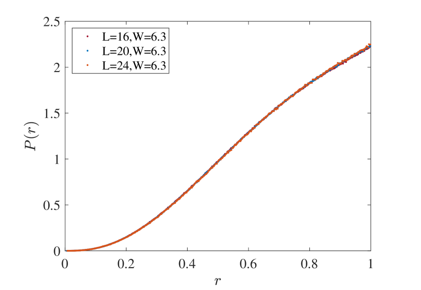
(a) $P(r)$ of the NH AM at the critical point

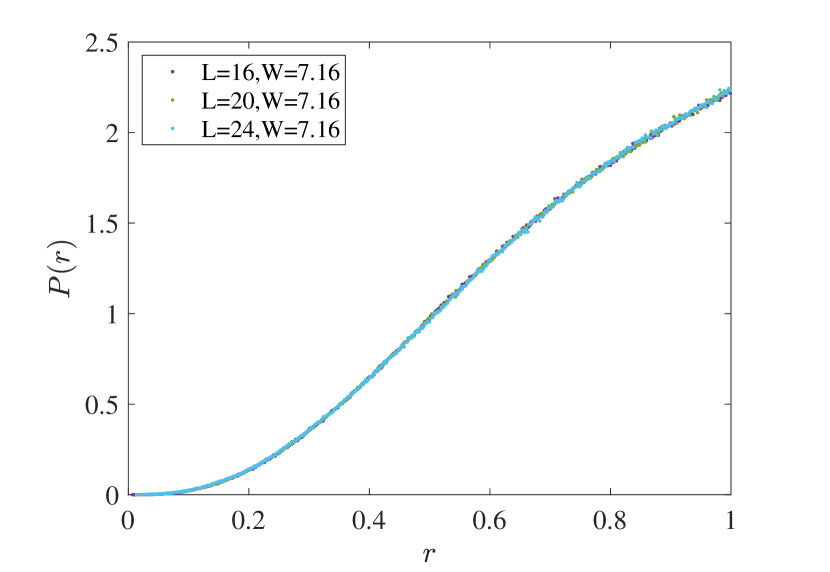
(b) $P(r)$ of the NH U(1) model at the critical point

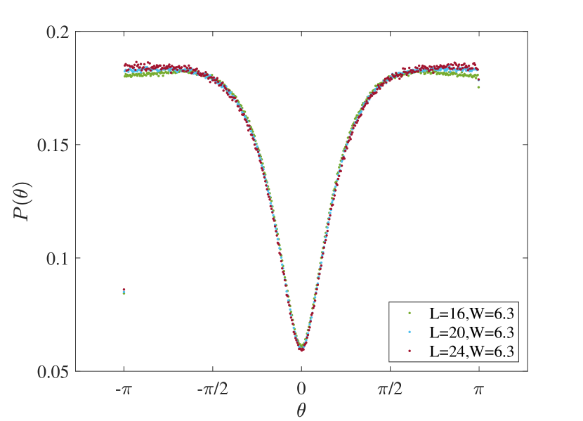
(c) $P(\theta)$ of the NH AM at the critical point

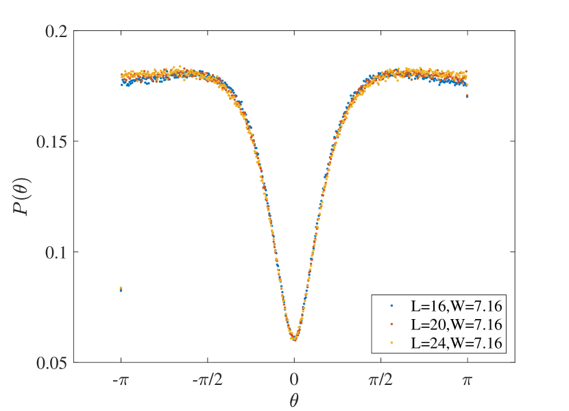
(d) $P(\theta)$ of the NH U(1) model at the critical point

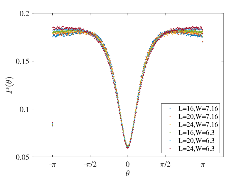
(e) critical $P(\theta)$ of the NH AM and U(1) model

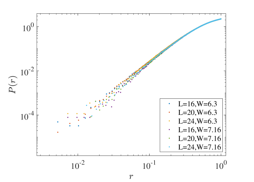
(f) critical $P(r)$ of the NH AM and U(1) model

Figure 12: $P(r)$ and $P(\theta)$ at the critical point. The statistics for the non-Hermitian (NH) Anderson model (AM) are taken over $M=1.2\times 10^{5}$, $6\times 10^{4}$, $10^{4}$ samples for the system size $L=16$, $20$, $24$, respectively. The statistics for NH U(1) model are taken over $M=2.5\times 10^{4}$, $1.2\times 10^{4}$, $6400$ samples for the system size $L=16$, $20$, $24$, respectively.

References

- Sondhi et al. (1997) S. L. Sondhi, S. M. Girvin, J. P. Carini, and D. Shahar, Rev. Mod. Phys. 69, 315 (1997).
- Anderson (1958) P. W. Anderson, Phys. Rev. 109, 1492 (1958).
- Abrahams et al. (1979) E. Abrahams, P. W. Anderson, D. C. Licciardello, and T. V. Ramakrishnan, Phys. Rev. Lett. 42, 673 (1979).
- Wegner (1976) F. J. Wegner, Zeitschrift fur Physik B 25, 327 (1976).
- Effetov et al. (1980) K. B. Effetov, A. I. Larkin, and D. E. Khmel’nitsukii, Soviet Phys. JETP 52, 568 (1980).
- Hikami et al. (1980) S. Hikami, A. I. Larkin, and Y. Nagaoka, Progress of Theoretical Physics 63, 707 (1980).
- Hikami (1981) S. Hikami, Phys. Rev. B 24, 2671 (1981).
- Altland and Zirnbauer (1997) A. Altland and M. R. Zirnbauer, Phys. Rev. B 55, 1142 (1997).
- Evers and Mirlin (2008) F. Evers and A. D. Mirlin, Rev. Mod. Phys. 80, 1355 (2008).
- Kramer and MacKinnon (1993) B. Kramer and A. MacKinnon, Reports on Progress in Physics 56, 1469 (1993).
- Slevin and Ohtsuki (2014) K. Slevin and T. Ohtsuki, New Journal of Physics 16, 015012 (2014).
- Slevin and Ohtsuki (1997) K. Slevin and T. Ohtsuki, Phys. Rev. Lett. 78, 4083 (1997).
- Slevin and Ohtsuki (2016) K. Slevin and T. Ohtsuki, Journal of the Physical Society of Japan 85, 104712 (2016).
- Asada et al. (2005) Y. Asada, K. Slevin, and T. Ohtsuki, Journal of the Physical Society of Japan 74, 238 (2005).
- Slevin and Ohtsuki (2009) K. Slevin and T. Ohtsuki, Phys. Rev. B 80, 041304 (2009).
- Asada et al. (2004) Y. Asada, K. Slevin, and T. Ohtsuki, Phys. Rev. B 70, 035115 (2004).
- Luo et al. (2018) X. Luo, B. Xu, T. Ohtsuki, and R. Shindou, Phys. Rev. B 97, 045129 (2018).
- Luo et al. (2020) X. Luo, B. Xu, T. Ohtsuki, and R. Shindou, Phys. Rev. B 101, 020202 (2020).
- Xu et al. (2016) B. Xu, T. Ohtsuki, and R. Shindou, Phys. Rev. B 94, 220403 (2016).
- Tzortzakakis et al. (2020) A. F. Tzortzakakis, K. G. Makris, and E. N. Economou, Phys. Rev. B 101, 014202 (2020).
- Wang and Wang (2020) C. Wang and X. R. Wang, Phys. Rev. B 101, 165114 (2020).
- Huang and Shklovskii (2020a) Y. Huang and B. I. Shklovskii, Phys. Rev. B 101, 014204 (2020a).
- Huang and Shklovskii (2020b) Y. Huang and B. I. Shklovskii, Phys. Rev. B 102, 064212 (2020b).
- Cao et al. (1999) H. Cao, Y. G. Zhao, S. T. Ho, E. W. Seelig, Q. H. Wang, and R. P. H. Chang, Phys. Rev. Lett. 82, 2278 (1999).
- Wiersma (2008) D. S. Wiersma, Nature Physics 4, 359 (2008).
- Wiersma (2013) D. S. Wiersma, Nature Photonics 7, 188 (2013).
- Konotop et al. (2016) V. V. Konotop, J. Yang, and D. A. Zezyulin, Rev. Mod. Phys. 88, 035002 (2016).
- Feng et al. (2017) L. Feng, R. El-Ganainy, and L. Ge, Nature Photonics 11, 752 (2017).
- El-Ganainy et al. (2018) R. El-Ganainy, K. G. Makris, M. Khajavikhan, Z. H. Musslimani, S. Rotter, and D. N. Christodoulides, Nature Physics 14, 11 (2018).
- Ozdemir et al. (2019) S. K. Ozdemir, S. Rotter, F. Nori, and L. Yang, Nat Mater 18, 783 (2019).
- Miri and Alù (2019) M.-A. Miri and A. Alù, Science 363 (2019), 10.1126/science.aar7709.
- Shen and Fu (2018) H. Shen and L. Fu, Phys. Rev. Lett. 121, 026403 (2018).
- Papaj et al. (2019) M. Papaj, H. Isobe, and L. Fu, Phys. Rev. B 99, 201107 (2019).
- Hatano and Nelson (1996) N. Hatano and D. R. Nelson, Phys. Rev. Lett. 77, 570 (1996).
- Kawabata and Ryu (2020) K. Kawabata and S. Ryu, “Nonunitary scaling theory of non-hermitian localization,” (2020), arXiv:2005.00604 .
- Kawabata et al. (2019) K. Kawabata, K. Shiozaki, M. Ueda, and M. Sato, Phys. Rev. X 9, 041015 (2019).
- Zhou and Lee (2019) H. Zhou and J. Y. Lee, Phys. Rev. B 99, 235112 (2019).
- Oganesyan and Huse (2007) V. Oganesyan and D. A. Huse, Phys. Rev. B 75, 155111 (2007).
- Sá et al. (2020) L. Sá, P. Ribeiro, and T. c. v. Prosen, Phys. Rev. X 10, 021019 (2020).
- Slevin and Ohtsuki (2018) K. Slevin and T. Ohtsuki, Journal of the Physical Society of Japan 87, 094703 (2018), https://doi.org/10.7566/JPSJ.87.094703 .
- Wigner (1951) E. P. Wigner, Mathematical Proceedings of the Cambridge Philosophical Society 47, 790â798 (1951).
- Dyson (1962a) F. J. Dyson, Journal of Mathematical Physics 3, 140 (1962a).
- Dyson (1962b) F. J. Dyson, Journal of Mathematical Physics 3, 1199 (1962b).
- Grobe et al. (1988) R. Grobe, F. Haake, and H.-J. Sommers, Phys. Rev. Lett. 61, 1899 (1988).
- Ginibre (1965) J. Ginibre, Journal of Mathematical Physics 6, 440 (1965), https://doi.org/10.1063/1.1704292 .
- Shklovskii et al. (1993) B. I. Shklovskii, B. Shapiro, B. R. Sears, P. Lambrianides, and H. B. Shore, Phys. Rev. B 47, 11487 (1993).
- (47) See Supplemental Material at [URL will be inserted by publisher].
- Atas et al. (2013) Y. Y. Atas, E. Bogomolny, O. Giraud, and G. Roux, Phys. Rev. Lett. 110, 084101 (2013).
- Rodriguez et al. (2011) A. Rodriguez, L. J. Vasquez, K. Slevin, and R. A. Römer, Phys. Rev. B 84, 134209 (2011).
- Chalker et al. (1996a) J. T. Chalker, I. V. Lerner, and R. A. Smith, Journal of Mathematical Physics 37, 5061 (1996a).
- Chalker et al. (1996b) J. T. Chalker, I. V. Lerner, and R. A. Smith, Phys. Rev. Lett. 77, 554 (1996b).
- Chalker et al. (1996c) J. T. Chalker, V. E. Kravtsov, and I. V. Lerner, Journal of Experimental and Theoretical Physics Letters 64, 386 (1996c).
- Bogomolny and Giraud (2011) E. Bogomolny and O. Giraud, Phys. Rev. Lett. 106, 044101 (2011).
- Braun et al. (1998) D. Braun, G. Montambaux, and M. Pascaud, Phys. Rev. Lett. 81, 1062 (1998).
- Ndawana et al. (2002) M. L. Ndawana, R. A. Romer, and M. Schreiber, The European Physical Journal B - Condensed Matter and Complex Systems 27, 399 (2002).
- Ghosh et al. (2017) S. Ghosh, C. Miniatura, N. Cherroret, and D. Delande, Phys. Rev. A 95, 041602 (2017).
- Zharekeshev and Kramer (1995) I. K. Zharekeshev and B. Kramer, Japanese Journal of Applied Physics 34, 4361 (1995).
- Kawarabayashi et al. (1996) T. Kawarabayashi, T. Ohtsuki, K. Slevin, and Y. Ono, Phys. Rev. Lett. 77, 3593 (1996).
- Batsch et al. (1996) M. Batsch, L. Schweitzer, I. K. Zharekeshev, and B. Kramer, Phys. Rev. Lett. 77, 1552 (1996).
- Hofstetter (1996) E. Hofstetter, Phys. Rev. B 54, 4552 (1996).
- Grobe and Haake (1989) R. Grobe and F. Haake, Phys. Rev. Lett. 62, 2893 (1989).
- Akemann et al. (2019) G. Akemann, M. Kieburg, A. Mielke, and T. c. v. Prosen, Phys. Rev. Lett. 123, 254101 (2019).
- Hamazaki et al. (2020) R. Hamazaki, K. Kawabata, N. Kura, and M. Ueda, Phys. Rev. Research 2, 023286 (2020).