Nonadiabatic phenomena in molecular vibrational polaritons

Abstract

Nonadiabatic phenomena are investigated in the rovibrational motion of molecules confined in an infrared cavity. Conical intersections (CIs) between vibrational polaritons, similar to CIs between electronic polaritonic surfaces, are found. The spectral, topological, and dynamic properties of the vibrational polaritons show clear fingerprints of nonadiabatic couplings between molecular vibration, rotation and the cavity photonic mode. Furthermore, it is found that for the investigated system, composed of two rovibrating HCl molecules and the cavity mode, breaking the molecular permutational symmetry, by changing ³⁵Cl to ³⁷Cl in one of the HCl molecules, the polaritonic surfaces, nonadiabatic couplings, and related spectral, topological, and dynamic properties can deviate substantially. This implies that the natural occurrence of different molecular isotopologues needs to be considered when modeling realistic polaritonic systems.

I Introduction

Cavity quantum electrodynamics (CQED) deals with the interaction of matter with a quantized light field enclosed in a cavity Miller et al. (2005); Walls and Milburn (2008). Experimental and theoretical studies have revealed that the quantum nature of the light can significantly modify the different chemical, physical or energetic properties of material structures Ruggenthaler et al. (2018); Herrera and Owrutsky (2020); Hutchison et al. (2012); Ebbesen (2016); Hertzog et al. (2019); Galego et al. (2015, 2016); Feist et al. (2018); Schäfer et al. (2018); Herrera and Spano (2016, 2017); Kowalewski et al. (2016a, b); Davidsson and Kowalewski (2020); Mandal and Huo (2019); Ribeiro et al. (2018a); Luk et al. (2017); Groenhof and Toppari (2018); Szidarovszky et al. (2018a); Csehi et al. (2019a, b); Vendrell (2018a, b); Gu and Mukamel (2020a); del Pino et al. (2015); Dunkelberger et al. (2016); Herrera and Spano (2018); Ahn et al. (2018); Thomas et al. (2016); Vergauwe et al. (2016); Chervy et al. (2018); Vergauwe et al. (2019); Thomas et al. (2019); Long and Simpkins (2015); Muallem et al. (2016); Damari et al. (2019); Campos-Gonzalez-Angulo et al. (2019); Kéna-Cohen and Yuen-Zhou (2019); Mandal et al. (2020); Ulusoy et al. (2019); Du et al. (2019); Gu and Mukamel (2020b); Szidarovszky et al. (2020). Most of the works consider only a single confined photonic mode in an optical or plasmonic cavity which can strongly interact with atoms, molecules or nano materials. The strong coupling regime is reached when the light–matter coupling is stronger than the loss of the cavity mode and the decay rates in the matter. In the case of molecules, the confined photonic mode of the cavity can efficiently couple both electronic or vibrational states, depending on the cavity mode wavelength. In the first situation the different electronic molecular states mix with the UV–visible cavity photon forming hybrid light–matter, so-called electronic or vibronic polariton states carrying both characters of matter and light. Several experimental and theoretical studies have demonstrated that this phenomenon gives rise to a variety of interesting effects such as modification of the chemical landscapes Hutchison et al. (2012); Ebbesen (2016); Galego et al. (2016); Ribeiro et al. (2018a), cavity-induced nonadiabatic phenomena Ruggenthaler et al. (2018); Galego et al. (2015); Feist et al. (2018); Kowalewski et al. (2016a, b); Davidsson and Kowalewski (2020); Szidarovszky et al. (2018a); Csehi et al. (2019a, b); Vendrell (2018a, b); Gu and Mukamel (2020a), controlling photochemistry Kowalewski et al. (2016a, b); Mandal and Huo (2019); Luk et al. (2017); Groenhof and Toppari (2018); Gu and Mukamel (2020a) , or intermolecular collective effects Mandal and Huo (2019); Ulusoy et al. (2019); Du et al. (2019); Gu and Mukamel (2020b); Szidarovszky et al. (2020).

Recently efforts have been made to study the vibrational strong coupling (VSC) within one molecular electronic state del Pino et al. (2015); Herrera and Spano (2018); Long and Simpkins (2015); Muallem et al. (2016); Ribeiro and Yuen-Zhou (2017); Campos-Gonzalez-Angulo et al. (2019); Kéna-Cohen and Yuen-Zhou (2019). In this regime experiments focus on the cavity-induced manipulation of chemical reactions in the ground electronic state or studying the effects of vibrational polaritons in solid and liquid phase inside infrared (IR) Fabry–Pérot cavities Dunkelberger et al. (2016); Ahn et al. (2018); Thomas et al. (2016); Vergauwe et al. (2016); Chervy et al. (2018); Vergauwe et al. (2019); Thomas et al. (2019). The presence of the vibrational strong coupling may lead to the suppression or enhancement of reactive pathways for molecules even in the absence of external photon pumping, implying that they involve thermally activated processes Vergauwe et al. (2019); Thomas et al. (2019); Campos-Gonzalez-Angulo et al. (2019); Kéna-Cohen and Yuen-Zhou (2019). As a necessary initial step to understand chemical reactivity, the detailed theoretical description and characterization of individual molecular vibrations interacting with an IR cavity mode also received focus Hernández and Herrera (2019); Triana et al. (2020).

In the present work we extend the theoretical approach by incorporating the effect of molecular rotation with vibrational polaritons. We employ realistic and highly-accurate molecular models, based on accurate quantum chemical and variational nuclear motion computations. This allows for a high-resolution insight into the formation, the spectroscopy and the dynamics of rovibrational polaritons, including cavity photon-mediated energy transfer between the different types of molecules. Because utilizing microfluidic cavities allows for the experimental realization of vibrational polaritons in the liquid phase, and because gas phase molecular polaritons are likely to be investigated eventually, special emphasis is given to the role of molecular rotations. The coupling strength between the cavity mode and the vibrational transition of the molecule naturally depends on the spatial orientation of the molecule. If molecular rotation is feasible, such as in the liquid or gas phase, then a simple averaging over different orientations is in principle erroneous, because the orientation dependent coupling strength couples the rotational degrees of freedom with the vibrational ones. Such couplings give rise to nonadiabatic effects Köppel et al. (1984); Yarkony (1996); Baer (2002); Worth and Cederbaum (2004); Domcke et al. (2004); Baer (2006) or in some cases to the formation of light-induced conical intersections (LICIs) Moiseyev et al. (2008); Halász et al. (2011, 2012) , which can have a significant impact on the polaritonic properties Szidarovszky et al. (2018a); Csehi et al. (2019a). The impact of simple orientational averaging has been investigated in the context of light-induced electronic conical intersections for example in Refs. Halász et al. (2014, 2015); Szidarovszky et al. (2018b). It is difficult to judge in general the error introduced by neglecting nonadiabatic coupling between rotations and vibrations in systems with vibrational strong coupling, because the error is strongly system specific. Nonetheless, it is an issue which should be considered.

We introduce the concept of vibrational potential energy surfaces, on which rotational dynamics proceed, and show the impact of the cavity-induced nonadiabatic coupling – between rotations and vibrations – on spectroscopic, dynamical and topological properties of molecules. Our showcase system is a mixture of H³⁵Cl and H³⁷Cl molecules interacting with a photonic mode.

II Theoretical approach

II.1 Rovibrational polaritons

The hamiltonian of rotating-vibrating molecules interacting with a single lossless cavity mode can be written in the dipole approximation as

$$\begin{split}\hat{H}=\sum_{i=1}^{N_{{\rm mol}}}(\hat{H}_{{\rm m}}^{(i)}-\hat{{\rm\mathbf{E}}}_{{\rm c}}\hat{\mathbf{\upmu}}^{(i)})+\hat{H}_{{\rm c}}=\\ \sum_{i=1}^{N_{{\rm mol}}}\big{(}\hat{H}_{{\rm m}}^{(i)}-\sqrt{\frac{\hbar\omega_{{\rm c}}}{\varepsilon_{0}V}}\mathbf{e}\hat{\mathbf{\upmu}}^{(i)}(\hat{a}_{{\rm c}}^{\dagger}+\hat{a}_{{\rm c}})\big{)}+\hbar\omega_{{\rm c}}\hat{a}_{{\rm c}}^{\dagger}\hat{a}_{{\rm c}}.\end{split}$$ (1)

where $\hat{H}_{{\rm m}}^{(i)}$ is the ith field-free molecular rovibrational Hamiltonian, $\hat{a}_{c}^{\dagger}$ and $\hat{a}_{c}$ are photon creation and annihilation operators, respectively, $\omega_{c}$ is the frequency of the cavity mode, $\hslash$ is Planck’s constant divided by $2\pi$, $\varepsilon_{0}$ is the electric constant, $V$ is the volume of the electromagnetic mode, $\mathbf{e}$ is the polarization vector of the cavity mode, and $\hat{\mathbf{\upmu}}^{(i)}$ is the dipole moment of the ith molecule.

We assume the cavity electric field to be polarized along the lab-fixed z-axis, $\mathbf{e}=(0,0,1)$, and we consider an IR cavity, which allows restricting the molecular model to a single electronic state. Then, the

$$|N\rangle\prod_{i=1}^{N_{{\rm mol}}}|\Psi_{{\rm rovib}}^{i,n_{i}J_{i}M_{i}}\rangle$$ (2)

direct-product functions, also called diabatic states, provide a complete basis, where the $|\Psi_{{\rm rovib}}^{i,nJM}\rangle$ field-free rovibrational eigenstates satisfy

$$\hat{H}_{{\rm m}}^{(i)}|\Psi_{{\rm rovib}}^{i,nJM}\rangle=E_{{\rm rovib}}^{(i),nJ}|\Psi_{{\rm rovib}}^{i,nJM}\rangle,$$ (3)

$J$ and $M$ are the rotational angular momentum and its projection onto the space-fixed z-axis, respectively, $n$ is all other quantum numbers uniquely defining the rovibrational states, and $|N\rangle$ is a photon number state of the cavity radiation. For a diatomic molecule $n$ can be identified with the single vibrational quantum number $v$, and using the notation $|\Psi_{{\rm rovib}}^{i,nJM}\rangle\equiv|v_{i}J_{i}M_{i}\rangle$, the matrix representation of Eq. (1) using the basis of Eq. (2) gives matrix elements of the following form:

$$\begin{split}&\Big{(}\langle N|\prod_{i=1}^{N_{{\rm mol}}}\langle v_{i}J_{i}M_{i}|\Big{)}\hat{H}\Big{(}\prod_{j=1}^{N_{{\rm mol}}}|v^{\prime}_{j}J^{\prime}_{j}M^{\prime}_{j}\rangle|N^{\prime}\rangle\Big{)}=\\ &\sum_{i=1}^{N_{{\rm mol}}}\delta_{M_{i}M^{\prime}_{i}}\Big{[}E_{{\rm rovib}}^{(i),v_{i}J_{i}}\delta_{v_{i}v^{\prime}_{i}}\delta_{J_{i}J^{\prime}_{i}}\delta_{NN^{\prime}}-\sqrt{\frac{\hbar\omega_{{\rm c}}}{\varepsilon_{0}V}}\langle v_{i}|\mu^{(i)}(R_{i})|v^{\prime}_{i}\rangle\langle J_{i}M_{i}|{\rm cos}(\theta_{i})|J^{\prime}_{i}M_{i}\rangle\times\\ &\Big{(}\sqrt{N}\delta_{NN^{\prime}+1}+\sqrt{N+1}\delta_{NN^{\prime}-1}\Big{)}\Big{]}\prod_{j\neq i}\delta_{v_{j}v^{\prime}_{j}}\delta_{J_{j}J^{\prime}_{j}}\delta_{M_{j}M^{\prime}_{j}}+N\hbar\omega_{{\rm c}}\delta_{NN^{\prime}}\prod_{j}^{N_{{\rm mol}}}\delta_{v_{j}v^{\prime}_{j}}\delta_{J_{j}J^{\prime}_{j}}\delta_{M_{j}M^{\prime}_{j}},\end{split}$$ (4)

where $\mu^{(i)}(R_{i})$ is the permanent dipole moment as a function of the internuclear distance $R_{i}$, $\theta_{i}$ is the angle between the space-fixed z axis and the ith molecule, and the energy scale was set so that the zero point energy of the photonic mode, $\hbar\omega_{{\rm c}}/2$, is omitted.

The rovibrational polaritonic states are the eigenstates of the Hamiltonian of Eq. (1). The kth polariton can be written as

$$|\Psi_{{\rm pol}}^{k}\rangle=\sum_{N}\sum_{v_{i},J_{i},M_{i}}C_{N,v_{1}J_{1}M_{1},...,v_{N_{{\rm mol}}}J_{N_{{\rm mol}}}M_{N_{{\rm mol}}}}^{k}\prod_{i}|v_{i}J_{i}M_{i}\rangle|N\rangle,$$ (5)

where $C_{N,v_{1}J_{1}M_{1},...,v_{N_{{\rm mol}}}J_{N_{{\rm mol}}}M_{N_{{\rm mol}}}}^{k}$ are the coefficients of the kth eigenvector of the matrix having the elements given in Eq. (4).

II.2 Computational details

The field-free rovibrational energies of the H³⁵Cl and H³⁷Cl molecules were computed as $E_{{\rm rovib}}^{(i),v_{i}J_{i}}=E_{{\rm vib}}^{(i),v_{i}}+B_{v_{i}}^{(i)}J(J+1)$, where the $E_{{\rm vib}}^{(i),v_{i}}$ vibrational energies were obtained from converged variational computations utilizing the spherical-DVR discrete variable representation (DVR) Szidarovszky et al. (2010) and the potential energy curve (PEC) of Ref. Magnier et al. (1993). The $B_{v}$ rotational constants (given in energy units) were evaluated for each vibrational state as $B_{v}^{(i)}=\langle v_{i}|\hbar^{2}/(2m_{{\rm red}}^{(i)}R^{2})|v_{i}\rangle$, where $m_{{\rm red}}^{(i)}$ is the reduced vibrational mass of the ith molecule. The nuclear masses used in the computations were $m_{{\rm H}}=1.00784$ u, $m_{{\rm{}^{35}Cl}}=34.9689$ u, and $m_{{\rm{}^{37}Cl}}=36.9659$ u.

For computing the $\langle v_{i}|\mu^{(i)}(R)|v^{\prime}_{i}\rangle\equiv\mu^{(i)}_{v_{i}v^{\prime}_{i}}$ vibrational (transition) dipole elements, the dipole moment curve of Ref. Zemke et al. (1981) was used. The values obtained are $\mu^{\rm(H^{35}Cl)}_{00}=0.42858$, $\mu^{\rm(H^{35}Cl)}_{10}=\mu^{\rm(H^{35}Cl)}_{01}=0.027055$, $\mu^{\rm(H^{37}Cl)}_{00}=0.42857$, and $\mu^{\rm(H^{37}Cl)}_{10}=\mu^{\rm(H^{37}Cl)}_{01}=0.027045$, all in atomic units. The $\langle J_{i}M_{i}|{\rm cos}(\theta)|J^{\prime}_{i}M_{i}\rangle$ terms were evaluated using an expression involving 3-j symbols,

$$\langle JM|{\rm cos}(\theta)|J^{\prime}M^{\prime}\rangle=\sqrt{(2J+1)(2J^{\prime}+1)}(-1)^{M^{\prime}}\footnotesize{\begin{pmatrix}J&1&J^{\prime}\\ M&0&-M^{\prime}\end{pmatrix}}\footnotesize{\begin{pmatrix}J&1&J^{\prime}\\ 0&0&0\end{pmatrix}},$$ (6)

which can be derived using the relations $\langle\phi,\theta|J\,M\rangle=Y_{JM}(\theta,\phi)=\sqrt{\frac{2J+1}{4\pi}}{D_{M0}^{J}}^{*}(\phi,\theta,\chi)$, ${\rm cos}(\theta)={D_{00}^{1}}(\phi,\theta,\chi)$, and $\int D_{K_{1}M_{1}}^{J_{1}}(\mathbf{\Omega})D_{K_{2}M_{2}}^{J_{2}}(\mathbf{\Omega})D_{K_{3}M_{3}}^{J_{3}}(\mathbf{\Omega})d\mathbf{\Omega}=8\pi^{2}\footnotesize{\begin{pmatrix}J_{1}&J_{2}&J_{3}\\ K_{1}&K_{2}&K_{3}\end{pmatrix}}\footnotesize{\begin{pmatrix}J_{1}&J_{2}&J_{3}\\ M_{1}&M_{2}&M_{3}\end{pmatrix}}$ Zare (1988), where $D_{KM}^{J}(\mathbf{\Omega})$ is the Wigner D-matrix and $\mathbf{\Omega}$ represents the three Euler angles $\phi$, $\theta$, and $\chi$.

III Results and discussion

III.1 Vibrational polaritonic energy surfaces (VPES)

For understanding the underlying physics, it is useful to construct the matrix representation of the Hamiltonian in Eq. (1) using vibrational-photonic basis functions $|N\rangle\prod_{i=1}^{N_{{\rm mol}}}|\Psi_{{\rm vib}}^{i,v_{i}}\rangle$. The matrix elements of the resulting vibro-photonic Hamiltonian depend on the $\theta$ rotational coordinates. After removing the rotational kinetic energy terms, the eigenvalues of the vibro-photonic Hamiltonian form vibrational polaritonic energy surfaces (VPES), which are functions of the $N_{{\rm mol}}$ rotational coordinates. Note the analogy that the VPESs provide effective potential energy surfaces (PES) for the rotational motion the same way as the usual light-dressed electronic potentials provide effective PESs for vibrational motion in polyatomics.

For two diatomic molecules (denoted as molecule 1 and 2, respectively) coupled to a single IR cavity mode, the first 4$\times$4 block in the vibro-photonic Hamiltonian reads

$$\mathbf{H}^{4\times 4}=\mathbf{T}_{{\rm rot}}+\mathbf{V}_{{\rm rot}},$$ (7)

where

$$\mathbf{T}_{{\rm rot}}=\begin{bmatrix}B_{0}^{(1)}\hat{T}_{{\rm rot}}^{(1)}+B_{0}^{(2)}\hat{T}_{{\rm rot}}^{(2)}&0&0&0\\ 0&B_{0}^{(1)}\hat{T}_{{\rm rot}}^{(1)}+B_{0}^{(2)}\hat{T}_{{\rm rot}}^{(2)}&0&0\\ 0&0&B_{1}^{(1)}\hat{T}_{{\rm rot}}^{(1)}+B_{0}^{(2)}\hat{T}_{{\rm rot}}^{(2)}&0\\ 0&0&0&B_{0}^{(1)}\hat{T}_{{\rm rot}}^{(1)}+B_{1}^{(2)}\hat{T}_{{\rm rot}}^{(2)}\end{bmatrix},$$ (8)

$$\begin{split}\mathbf{V}_{{\rm rot}}&=\begin{bmatrix}E_{{\rm vib}}^{(1),0}+E_{{\rm vib}}^{(2),0}&0&0&0\\ 0&E_{{\rm vib}}^{(1),0}+E_{{\rm vib}}^{(2),0}+\hbar\omega_{{\rm c}}&0&0\\ 0&0&E_{{\rm vib}}^{(1),1}+E_{{\rm vib}}^{(2),0}&0\\ 0&0&0&E_{{\rm vib}}^{(1),0}+E_{{\rm vib}}^{(2),1}\end{bmatrix}-\sqrt{\hbar\omega_{{\rm c}}/(\varepsilon_{0}V)}\times\\ &\begin{bmatrix}0&\mu_{00}^{(1)}{\rm cos}(\theta_{1})+\mu_{00}^{(2)}{\rm cos}(\theta_{2})&0&0\\ \mu_{00}^{(1)}{\rm cos}(\theta_{1})+\mu_{00}^{(2)}{\rm cos}(\theta_{2})&0&\mu_{01}^{(1)}{\rm cos}(\theta_{1})&\mu_{01}^{(2)}{\rm cos}(\theta_{2})\\ 0&\mu_{10}^{(1)}{\rm cos}(\theta_{1})&0&0\\ 0&\mu_{10}^{(2)}{\rm cos}(\theta_{2})&0&0\end{bmatrix},\end{split}$$ (9)

where $\mu_{kl}^{(i)}=\langle v_{i}=k|\mu^{(i)}(R)|v_{i}=l\rangle$, $\hat{T}_{{\rm rot}}^{(i)}$ is the squared rotational angular momentum of the ith molecule, and $B_{v}^{(i)}$ is the rotational constant of the ith molecule in its vth vibrational state. For the specific case of a H³⁵Cl and a H³⁷Cl molecule, Figure 1 show the three largest eigenvalues of the $\mathbf{V}_{{\rm rot}}$ matrix in Eq. (9) as a function of the $\theta_{i}$ variables for a coupling strength of $\mu^{\rm(H^{35}Cl)}_{00}\sqrt{\hbar\omega_{{\rm c}}/(\varepsilon_{0}V)}=33.26$ cm^-1. The same is shown in Fig. 2 for the case of two identical H³⁵Cl molecules. Fig. 1 demonstrates that in the case of the two different isotopologues, three polaritons are formed, as expected Houdré et al. (1996); Szidarovszky et al. (2020), and conical intersections (CI) can be formed between the VPESs. In the case of two identical H³⁵Cl molecules, Fig. 2 shows that the middle polaritonic surface is flat, which one would usually identify as a dark polaritonic state (although it is not dark in this case, see below). The upper (lower) VPES touches the dark state for red (blue) shifted cavity wave lengths.

III.2 Topological properties

A well-known consequence of CIs or LICIs between adiabatic electronic PESs is that the electronic wave functions of the connected surfaces become double valued, i.e., propagating the electronic wave function of a single surface along a closed curve around the CI leads to the accumulation of a topological phase of $\pi$ Longuet-Higgins et al. (1958); Longuet-Higgins (1961); Mead and Truhlar (1982); Berry (1984); Halász et al. (2011, 2018). In order to verify that the LICIs between VPESs are indeed true LICIs (and to confirm the existence of LICIs between VPESs even when the diagonal dipole terms are not omitted from the VPESs), the numerical verification of the topological phases was carried out. Now, we borrow a well-established framework developed for natural nonadiabatic phenomena, which was succesfully applied to study the topological properties of “natural” electronic degeneracies Baer (1975, 2002); Vértesi et al. (2005); Baer (2006).

Let us start from the adiabatic-to-diabatic transformation (ADT)

$$\mathbf{W}=\mathbf{A}^{\dagger}\mathbf{VA}$$ (10)

where $\mathbf{W}$ and $\mathbf{V}$ denote the diabatic and adiabatic PES, respectively. $\mathbf{A}$ is a unitary matrix called ADT matrix, which can be obtained by solving the equation

$$\nabla\mathbf{A}+\bm{\tau}\mathbf{A}=0.$$ (11)

Its solution can be written in the following form

$$\mathbf{A}(s)=\gamma\,exp\left(-\int_{s_{0}}^{s}\bm{\tau}(s)\,ds\right)\mathbf{A}(s_{0})$$ (12)

where $\gamma$ is a path ordering operator and $\bm{\tau}(s)$ is the nonadiabatic coupling matrix which contains the nonadibatic coupling terms (NAC)s

$$\bm{\tau}_{i,j}=<\Psi_{i}|\nabla|\Psi_{j}>.$$ (13)

Here $\Psi_{i}$ and $\Psi_{j}$ are $ith$ and $jth$ adiabatic vibrational wave functions, respectively and $\nabla$ is the gradient operator corresponding to the rotational coordinates.

The necessary condition for the $\mathbf{A}$-matrix to yield single-valued diabatic wave function is that the $\mathbf{D}$-matrix,

$$D(\Gamma)=\gamma\,exp\left(-\oint_{\Gamma}\bm{\tau}\,ds\right)$$ (14)

needs to be diagonal and has, in its diagonal, numbers of ($+1$)s or ($-1$)s. The number of ($-1$)s in the $\mathbf{D}$ is designated as $K$ which is the number of the adiabatic vibrational eigenfunctions that flip their sign. The $\mathbf{D}$-matrix is the topological matrix which contains all topological features of a vibrational manifold in a region surrounded by its contour $\varGamma$ and $K$ is the topological number. The positions of the ($-1$)s in the $\mathbf{D}$-matrix correspond with the vibrational eigenfunctions that flip their sign. The equation for $\mathbf{D}(\Gamma)$ is a kind of quantization condition to be fulfilled by the nonadiabatic coupling matrix $\bm{\tau}$ along any closed contour $\varGamma$ in configuration space (CP).

In case of two quasi-isolated adiabatic states ($j,j+1$) the quantization condition reads:

$$\alpha_{j,j+1}(\Gamma)=\oint_{\Gamma}\bm{\tau}_{j,j+1}(s|\Gamma)\,ds=n_{j}\,\pi$$ (15)

where $\alpha_{j,j+1}(\Gamma)$ is the topological phase. When the closed contour $\Gamma$ is a circle with radii q:

$$\alpha_{j,j+1}(q)=\int_{0}^{2\pi}\bm{\tau}_{j,j+1}(\varphi|q)d\varphi.$$ (16)

The adiabatic-to-diabatic transformation angle can be defined as:

$$\gamma_{j,j+1}(\varphi|q)=\int_{0}^{\varphi}\bm{\tau}_{\varphi j,j+1}(\varphi|q)d\varphi.$$ (17)

In the related numerical calculations of this study we concentrate on LICIs between the lower and middle as well as the middle and upper vibrational polaritonic states (see Figs. 1 and 2). In Figure 1 these are the two (1,2) and two (2,3) LICIs, corresponding to the three bright states, which are formed for the “H³⁵Cl + H³⁷Cl + IR cavity mode” system. These are “true” LICIs, i.e., first-order degeneracy points, as the two HCl molecules are distinguishable. However, for the two indistinguishable confined H³⁵Cl molecules, only a second-order degeneracy point is formed, as demonstrated in Fig. 2.

In Fig. 3 we report on results for the “H³⁵Cl + H³⁷Cl + IR cavity mode” system. At first we calculated the $\bm{\tau}_{1,2}$ along a circle located at the (1,2)LICI point. In Fig. 3. panel A the related ADT angle $\gamma_{1,2}$ and the corresponding topological phase $\alpha_{1,2}=-1.0169\pi$ are shown. Similar quantities are presented for the (2,3)LICI in panel B. Here we obtain $\alpha_{2,3}=1.0077\pi$. It is well noticed that both $\alpha_{1,2}$ and $\alpha_{2,3}$ are close to $\pi$ as expected. This means that there is only one (1,2)LICI and one (2,3)LICI in the studied CS region of panel A and B, respectively, and the two-state approximation works well. In panel C the closed contour, in contrast to the two previous ones, surrounds two LICI points. The calculated $\alpha_{1,2}=-1.1227\pi$ and $\alpha_{2,3}=-0.3436\pi$ topological phases are far from being close to $\pi$, indicating that the two-state approximation fails to describe accurately the topological behavior. The third state is needed to be involved in the calculations for the proper topological description. In order to derive the three-state ADT matrix elements and the corresponding $\mathbf{D}$ matrix one has to calculate all off-diagonal matrix elements of the $\bm{\tau}(s)$ NAC matrix and then apply Eqs. 12 and 14. On panel D of Fig. 3 the values for the $\mathbf{D}$ matrix elements are presented for the closed curve indicated as an inset in the panel. The values of the diagonal elements ($-1$,$+1$,$-1$) clearly imply that the distribution contains an odd number (presumably one) of LICI for each type (1,2)LICI and (2,3)LICI. Therefore, the first and third vibrational wave functions change their sign while the sign of the second vibrational wave function remains unchanged after flipping its sign twice.

In Fig. 4 topological results are presented for the “2$\times$H³⁵Cl + IR cavity mode” system in which, due to the symmetry, only a second-order degeneracy point is formed (see on Fig. 2). Consequently, if the two-state approximation worked, one would have to obtain $2\pi$ for the value of the topological phase $\alpha_{1,2}$. Instead, we obtained values of $\alpha_{1,2}=1.0878\pi$ and $\alpha_{2,3}=1.6789\pi$, which clearly show that the two-state approximation does not work in the studied region of the CS. At this point, one has to derive again the three-state ADT matrix elements and the corresponding $\mathbf{D}$ matrix by employing the appropriate nonadiabatic coupling terms. The obtained ($1$,$1$,$1$) values in the diagonal of the $\mathbf{D}$ matrix clearly demonstrate that the three-state approximation works perfectly and none of the vibrational wave functions change sign.

The above studies undoubtedly proved that the topological features of VPES and electronic PES are very similar. Earlier results Baer (2002); Vértesi et al. (2005); Baer (2006) obtained for the latter situation can almost be transferred one by one so as to understand the topological features of the VPESs. The topological properties of the VPESs imply that direct observables should exist, which prove the existence of the nonadiabatic effects among the VPESs. Some of these are presented in the following sections.

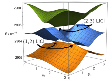
Figure 1: Vibrational polaritonic energy surfaces (VPES) of the “H³⁵Cl + H³⁷Cl + IR cavity mode” system, obtained by diagonalizing the $\mathbf{V}_{{\rm rot}}$ matrix in Eq. (9) using the parameters $E_{{\rm vib}}^{1,0}+E_{{\rm vib}}^{2,0}+\hbar\omega_{{\rm c}}=2904.5$ cm^-1, $E_{{\rm vib}}^{1,1}+E_{{\rm vib}}^{2,0}=2905.9$ cm^-1, and $E_{{\rm vib}}^{1,0}+E_{{\rm vib}}^{2,1}=2903.7$ cm^-1. The $\mu^{\rm(H^{35}Cl)}_{00}\sqrt{\hbar\omega_{{\rm c}}/(\varepsilon_{0}V)}$ coupling strength is 33.26 cm^-1. Two types of light-induced conical intersections (LICI) are also highlighted, see text.

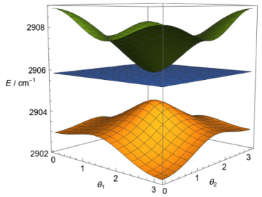
Figure 2: Same as Fig. 1, but for two identical H³⁵Cl molecules in the cavity. The parameters are $E_{{\rm vib}}^{1,1}+E_{{\rm vib}}^{2,0}=E_{{\rm vib}}^{1,0}+E_{{\rm vib}}^{2,1}=2905.9$ cm^-1, $\mu^{\rm(H^{35}Cl)}_{00}\sqrt{\hbar\omega_{{\rm c}}/(\varepsilon_{0}V)}=33.26$ cm^-1, while $E_{{\rm vib}}^{1,0}+E_{{\rm vib}}^{2,0}+\hbar\omega_{{\rm c}}=2904.5$ cm^-1.

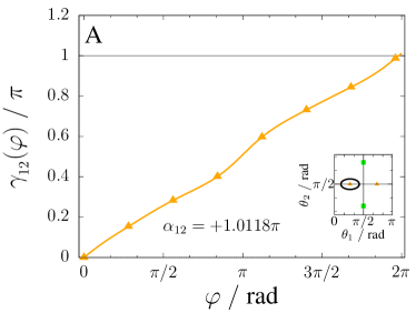
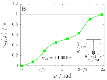
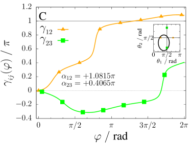
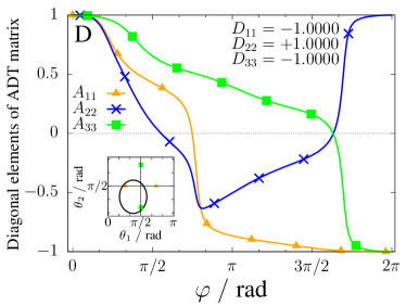
Figure 3: The adiabatic-to-diabatic transformation angle $\gamma_{i,j}$ (on panels A, B and C) and the diagonal elements of the A-topological matrix (on panel D) as a function of $\varphi\in[0,2\pi]$. $\varphi$ defines the position on the closed curve. The topological phase $\alpha_{i,j}$ and the $D$-topological matrix elements are both shown for the “H³⁵Cl + H³⁷Cl + IR cavity mode” system.

.

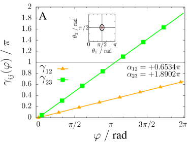
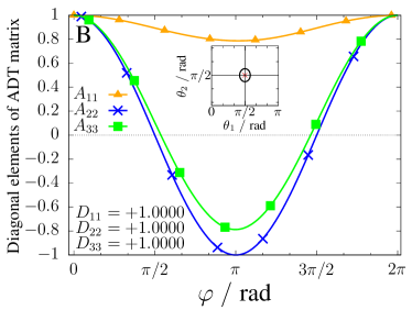
Figure 4: The adiabatic-to-diabatic transformation angle $\gamma_{i,j}$ (panel A) and the diagonal elements of the A-topological matrix (panel B) as a function of $\varphi\in[0,2\pi]$. $\varphi$ defines the position on the closed curve. The topological phase $\alpha_{i,j}$ and the $D$-topological matrix elements are both shown for the “2$\times$H³⁵Cl + IR cavity mode” system.

III.3 Light-dressed spectroscopy

Another physical property which can be effected by CIs or LICIs is the spectrum. The spectroscopy of polaritonic systems is a valuable tool for providing insight into their various physiochemical properties Zeb et al. (2018); Ribeiro et al. (2018b); Szidarovszky et al. (2018a, 2020), and nonadiabatic effects resulting from the strong coupling of the electronic, vibrational, rotational, and photonic degrees of freedom can cause a significant modification on the molecular absorption spectra. In one possible theoretical formulation of light-dressed spectroscopy Szidarovszky et al. (2019), transitions between light-dressed states are evaluated using first-order time-dependent perturbation theory, that is, for the $T_{l\leftarrow k}$ transition amplitude between the kth and lth light-dressed state $T_{l\leftarrow k}\propto\langle\Psi_{l}|\hat{\mathbf{d}}\mathbf{e}^{(p)}|\Psi_{k}\rangle\delta(E_{l}-E_{k}\pm\hbar\omega_{p})$ is assumed, where $\mathbf{e}^{(p)}$ and $\hbar\omega_{p}$ are the polarization vector and photon energy of the probe pulse, respectively, while $|\Psi_{i}\rangle$ and $E_{i}$ are the light-dressed wave functions and energies, respectively. In this work the light-dressed states (polaritonic states), $|\Psi_{i}\rangle$, have the form shown in Eq. (5), and the $T_{l\leftarrow k}$ transition amplitudes can be computed with formulae similar to that in Eq. (4). Note that within this framework the computed spectra represent the absorption of light running parallel to the cavity mirrors, in the medium, not that of which is transmitted through the mirrors.

Figure 5 shows the IR absorption spectra of H³⁵Cl molecules and the mixture of H³⁵Cl and H³⁷Cl molecules, confined in IR cavities of different coupling strengths. Blue, red, and green colors in the transition lines represent vibrational excitation in H³⁵Cl, vibrational excitation in the other H³⁵Cl (left panels) or H³⁷Cl (right panels), and photonic excitation, respectively. The color of each transition line is obtained by mixing the above three colors according to the weight of the different types of basis functions in the final polaritonic states of the transition. The panel (A1) in Fig. 5 demonstrates that at the weakest coupling strength presented in this work, the light-dressed spectrum of two confined H³⁵Cl molecules shows one dominant and several minor peaks, arising from the splitting of the single $|v=1,\,J=1,\,M=0\rangle\leftarrow|v=0,\,J=0,\,M=0\rangle$ field-free transition. The strongest peak is split into two in panel (B1) of Fig. 5. The small energy splitting reflects the slight differences in the rovibrational energies of H³⁵Cl and H³⁷Cl, while the significant difference in the peak heights reflects the different VPES landscape and related nonadiabatic effects (under field-free conditions the height of the split peak is nearly identical). The small green peaks represent excitation in the photonic mode (photon number increased by one), which appears in the spectrum due to the contamination of the photonic mode with molecular excited (ro)vibrational states, having non-zero transition amplitude. No significant difference can be seen in the low-resolution envelopes of the two panels in the first row.

The light dressed spectra at larger cavity coupling strengths demonstrate that the individual peak positions and peak heights can be slightly different for the confined 2$\times$H³⁵Cl and H³⁵Cl+H³⁷Cl systems, but no significant differences arise in their spectrum envelope. Due to the strong mixing between the different molecular excitations and the photonic mode, assigning the peaks at larger cavity coupling strengths becomes complicated and less informative. Nonetheless, the peak colors represent the character of the different transitions to some extent. Panels (B2),(B3) and (B4) of Fig. 5 show that some peaks are dominated by a H³⁵Cl, H³⁷Cl or photonic transition (peaks with mostly red, blue or green color), but other peaks show significant mixing between the rovibrational modes of the HCl molecules and the photonic mode (purple, dark green or brown peaks). Despite the subtle differences in the spectra of the “2$\times$H³⁵Cl + cavity mode” and “H³⁵Cl + H³⁷Cl cavity mode” systems, some of which can be attributed to the nonadiabatic couplings between the VPESs, the low-resolution spectrum envelopes remain nearly identical, thus the IR spectrum doesn’t seem to be the most efficient tool to highlight the nonadiabatic effects in this case.

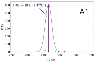
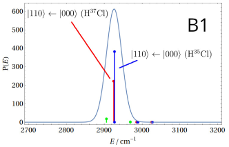
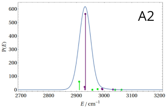
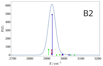
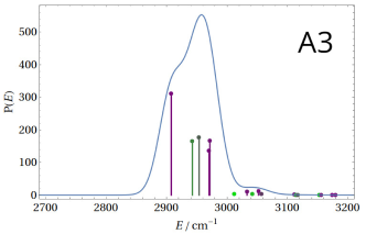
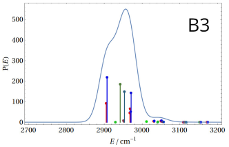
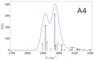
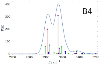
Figure 5: Light-dressed spectrum of the “2$\times$H³⁵Cl + IR cavity mode” system (panels A1, A2, A3 and A4) and “H³⁵Cl + H³⁷Cl + IR cavity mode” system (panels B1, B2, B3 and B4). See text for discussion on the peak assignment. Parameters are $E_{{\rm vib}}^{1,0}+E_{{\rm vib}}^{2,0}+\hbar\omega_{{\rm c}}=2904.5$ cm^-1, $E_{{\rm vib}}^{1,1}+E_{{\rm vib}}^{2,0}=2905.9$ cm^-1, $E_{{\rm vib}}^{1,0}+E_{{\rm vib}}^{2,1}=2903.7$ cm^-1, and the values of the coupling strength $\mu^{\rm(H^{35}Cl)}_{00}\sqrt{\hbar\omega_{{\rm c}}/(\varepsilon_{0}V)}$ equal 66.6, 133.2, 199.8, and 266.4 cm^-1 in the different rows from top to bottom, in order.

III.4 Laser-induced dynamics

An additional approach to highlight nonadiabatic couplings in molecular systems is to investigate their laser-induced dynamics. In this work such simulations were carried out by directly solving the time-dependent Schrödinger equation in the diabatic direct-product basis representation, assuming $T=0$ K. At room temperature, due to the non-zero populations in $J>0$ rotational levels, the numerical values for the expectation values shown below would vary, but the qualitative conclusions should not change.

As already demonstrated for the vibrational dynamics on electronic PESs Halász et al. (2011), an efficient way to pinpoint nonadiabatic effects is to monitor the populations on the adiabatic surfaces during the dynamics. Here we perform similar studies for the case of adiabatic vibrational polaritons. In the case of VPESs, the population on the $a$th adiabatic state is evaluated as

$$p^{(a)}=|\hat{P}^{(a)}|\Psi(t)\rangle|^{2},$$ (18)

where $|\Psi(t)\rangle$ is the time-dependent wave function expanded in terms of the direct-product diabatic states, see Eq. (2), and $\hat{P}^{(a)}=|\psi^{(a)}\rangle\langle\psi^{(a)}|$ is a projector onto the $a$th adiabatic state, i.e., the $a$th eigenstate of the matrix in Eq. (9). Note that

$$|\psi^{a}\rangle=\sum_{N,v_{1},v_{2}}{C_{N,v_{1},v_{2}}^{(a)}(\theta_{1},\theta_{2})|N\rangle|\Psi_{{\rm vib}}^{1,v_{1}}\rangle|\Psi_{{\rm vib}}^{2,v_{2}}\rangle},$$ (19)

that is, the $C_{N,v_{1},v_{2}}^{(a)}(\theta_{1},\theta_{2})$ expansion coefficients depend on the rotational coordinates, $\theta_{1}$ and $\theta_{2}$, as predictable from Figs. 1 and 2.

Fig. 6 shows the temporal evolution of the adiabatic populations for the “2$\times$H³⁵Cl + IR cavity mode” system and the “H³⁵Cl + H³⁷Cl + IR cavity mode” system, when a short IR laser pulse, tuned to the field-free vibrational fundamental of H³⁵Cl (2926.1 cm^-1), is used to excite these systems from their ground states. After 60 fs, when the laser field has subsided, the population of the ground adiabatic state is 0.52 for both systems, indicating that the degree of laser-induced molecular vibrational excitation is identical for the two systems. For both the “2$\times$H³⁵Cl + IR cavity mode” and “H³⁵Cl + H³⁷Cl + IR cavity mode” systems, shown in the the upper and lower panels of Fig. 6, respectively, the laser populates all three excited adiabatic states. However, the population is distributed among the three excited adiabatic states in a different manner for the two systems. Somewhat surprisingly, the middle polaritons, which one would intuitively address as dark states, are also populated by the light field for both systems. This is due to the permanent dipole coupling with the ground adiabatic state (see first row and column of second matrix in Eq. (9)), test simulations without this coupling show that the middle polaritons are indeed almost “dark”, and are much less populated. In either case, due to the strong nonadiabatic couplings between the VPESs, rapid, hundred-femtosecond timescale population transfer proceeds among all three adiabatic states following the excitation by the laser field. Overall, Fig. 6 demonstrates that when molecular rotations are feasable, strong nonadiabatic couplings influence the dynamics of multimolecule (ro)vibrational polaritons. Furthermore, the nonadiabatic dynamics shown in Fig. 6 verify that breaking the molecular permutational symmetry, in this case by introducing a different Cl isotope, the polariton dynamics can deviate substantially.

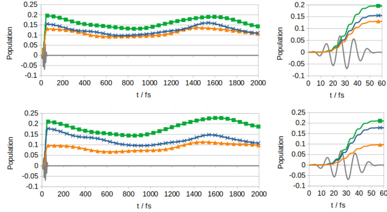
Figure 6: Adiabatic populations in the laser-induced dynamics of the “2$\times$H³⁵Cl + IR cavity mode” system (upper panels) and “H³⁵Cl + H³⁷Cl + IR cavity mode” system (lower panels). Squares, crosses, and triangles stand for the upper, middle, and lower adiabatic polaritonic VPESs, respectively, color coded according to Figs. 1 and 2. The continuous line represents the electric field of the laser pulse. Parameters are $E_{{\rm vib}}^{1,0}+E_{{\rm vib}}^{2,0}+\hbar\omega_{{\rm c}}=2904.5$ cm^-1, $E_{{\rm vib}}^{1,1}+E_{{\rm vib}}^{2,0}=2905.9$ cm^-1, $E_{{\rm vib}}^{1,0}+E_{{\rm vib}}^{2,1}=2903.7$ cm^-1, and $\mu^{\rm(H^{35}Cl)}\sqrt{\hbar\omega_{{\rm c}}/(\varepsilon_{0}V)}=133.2$ cm^-1. The pump laser has a field strength of $0.1/\sqrt{2}$ a.u., and its central wavenumber equals the field-free $|11\rangle\leftarrow|00\rangle$ rovibrational transition of H³⁵Cl (2926.1 cm^-1).

As an alternative approach to probe the presence of nonadiabatic couplings in the laser-induced dynamics of our rovibrational polaritonic test systems, the orientation, i.e., the $\langle{\rm cos}(\theta)\rangle$ expectation value, was evaluated for a single H³⁵Cl (H³⁷Cl) molecule, when confined in an IR cavity with another H³⁵Cl (H³⁷Cl) molecule or a H³⁷Cl (H³⁵Cl) isotopologue. The numerical results are shown for the same and mixed isotopologue cases in the upper and lower panels of Figure 7, respectively. The upper panel of Figure 7 demonstrates that the isotope effect causes only minor differences in the orientation dinamics, the curves for H³⁵Cl and H³⁷Cl and nearly identical. However, the lower panel of Figure 7 shows that on the timescale of the rotational dynamics of HCl (picoseconds), the orientation curves deviate substantially when the two isotopologues are mixed in the cavity. Although the exact value of the numerical results presented here should be treated with caution, because cavity loss was neglected in this work, such a dependence of the orientation on the partner molecule is a clear fingerprint of molecular distinguishability on the VPESs (and corresponding nonadiabatic couplings) and, therefore, on the rotational dynamics.

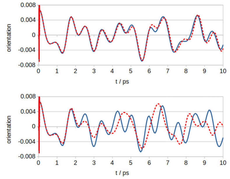
Figure 7: Upper panel: the laser-induced orientation, i.e., the $\langle{\rm cos}(\theta)\rangle$ expectation value of a confined H³⁵Cl molecule (blue continuous line) or a confined H³⁷Cl molecule (red dashed line), when sharing the cavity with an identical isotopologue, i.e., with a H³⁵Cl and a H³⁷Cl, respectively. Lower panel: the laser-induced orientation of H³⁵Cl (blue continuous line) and H³⁷Cl (red dashed line) in the “H³⁵Cl + H³⁷Cl + IR cavity mode” system. The inverse rotational constant in time units is 0.509 ps and 0.510 ps for H³⁵Cl and H³⁷Cl, respectively. $\mu^{\rm(H^{35}Cl)}\sqrt{\hbar\omega_{{\rm c}}/(\varepsilon_{0}V)}=133.2$ cm^-1, all other parameters are the same as in Fig. 6.

IV Summary and conclusions

A general framework for computing the rovibrational polaritons of several molecules in a lossless cavity was presented. Based on this formulation, the concept of vibrational potential energy surfaces (VPES) was introduced, which provide effective potential energy surfaces for the rotational motion of the confined molecules. For the test system of two rovibrating HCl molecules interacting with a single lossless infrared cavity mode, degeneracies were identified between the VPESs: light-induced conical intersections (LICI) were found when two different isotopologoues, H³⁵Cl and H³⁷Cl, are in the cavity, and a second-order degeneracy was found in the case of two same isotopologoues. The degeneracies between the VPESs were characterized based on their topological properties, and their nonadiabatic fingerprints were identified in the light-dressed spectra and the laser-induced dynamical properties of the investigated rovibrational polaritons.

The presented results clearly show that breaking molecular permutational symmetry due to different isotopes can play an important role in rovibrational polaritonic properties; the polaritonic surfaces, nonadiabatic couplings, and related spectral, topological, and dynamic properties can be influenced substantially. This implies that the natural abundance of different isotopologoues should be accounted for if one aims for a realistic simulation on confined molecular ensembles.

V Acknowledgement

This research was supported by the EU-funded Hungarian grant EFOP-3.6.2-16-2017-00005 as well as by the János Bolyai Research Scholarship of the Hungarian Academy of Sciences and by the ÚNKP-20-5 New National Excellence Program of the Ministry for Innovation and Technology from the source of the National Research, Development and Innovation Fund. The authors are grateful to NKFIH for support (Grants No. PD124623, K128396 and FK134291).

Data availability

The data that support the findings of this study are available from the corresponding author upon reasonable request.

References

- Miller et al. (2005) R. Miller, T. E. Northup, K. M. Birnbaum, A. Boca, A. D. Boozer, and H. J. Kimble, Journal of Physics B: Atomic, Molecular and Optical Physics 38, S551 (2005).
- Walls and Milburn (2008) D. F. Walls and G. J. Milburn, Quantum Optics, Berlin Heidelberg (Springer, 2008).
- Ruggenthaler et al. (2018) M. Ruggenthaler, N. Tancogne-Dejean, J. Flick, H. Appel, and A. Rubio, Nat. Rev. Chem. 2, 0118 (2018).
- Herrera and Owrutsky (2020) F. Herrera and J. Owrutsky, The Journal of Chemical Physics 152, 100902 (2020).
- Hutchison et al. (2012) J. A. Hutchison, T. Schwartz, C. Genet, E. Devaux, and T. W. Ebbesen, Angew. Chem. Int. Ed. 51, 1592 (2012).
- Ebbesen (2016) T. W. Ebbesen, Acc. Chem. Res. 49, 2403 (2016).
- Hertzog et al. (2019) M. Hertzog, M. Wang, J. Mony, and K. Börjesson, Chemical Society Reviews 48, 937 (2019).
- Galego et al. (2015) J. Galego, F. J. Garcia-Vidal, and J. Feist, Phys. Rev. X 5, 1 (2015).
- Galego et al. (2016) J. Galego, F. J. Garcia-Vidal, and J. Feist, Nat. Commun. 7, 13841 (2016).
- Feist et al. (2018) J. Feist, J. Galego, and F. J. Garcia-Vidal, ACS Photonics 5, 205 (2018).
- Schäfer et al. (2018) C. Schäfer, M. Ruggenthaler, and A. Rubio, Physical Review A 98 (2018), 10.1103/physreva.98.043801.
- Herrera and Spano (2016) F. Herrera and F. C. Spano, Phys. Rev. Lett. 116, 238301 (2016).
- Herrera and Spano (2017) F. Herrera and F. C. Spano, Phys. Rev. Lett. 118, 223601 (2017).
- Kowalewski et al. (2016a) M. Kowalewski, K. Bennett, and S. Mukamel, J. Chem. Phys. 144, 054309 (2016a).
- Kowalewski et al. (2016b) M. Kowalewski, K. Bennett, and S. Mukamel, J. Phys. Chem. Lett. 7, 2050 (2016b).
- Davidsson and Kowalewski (2020) E. Davidsson and M. Kowalewski, The Journal of Physical Chemistry A 124, 4672 (2020).
- Mandal and Huo (2019) A. Mandal and P. Huo, The Journal of Physical Chemistry Letters 10, 5519 (2019).
- Ribeiro et al. (2018a) R. F. Ribeiro, L. A. Martínez-Martínez, M. Du, J. Campos-Gonzalez-Angulo, and J. Yuen-Zhou, Chem. Sci. 9, 6325 (2018a).
- Luk et al. (2017) H. L. Luk, J. Feist, J. J. Toppari, and G. Groenhof, J. Chem. Theory Comput. 13, 4324 (2017).
- Groenhof and Toppari (2018) G. Groenhof and J. J. Toppari, J. Phys. Chem. Lett. 9, 4848 (2018).
- Szidarovszky et al. (2018a) T. Szidarovszky, G. J. Halász, A. G. Császár, L. S. Cederbaum, and Á. Vibók, J. Phys. Chem. Lett. 9, 6215 (2018a).
- Csehi et al. (2019a) A. Csehi, M. Kowalewski, G. J. Halász, and Á. Vibók, New J. Phys. 21, 093040 (2019a).
- Csehi et al. (2019b) A. Csehi, Á. Vibók, G. J. Halász, and M. Kowalewski, Physical Review A 100 (2019b), 10.1103/physreva.100.053421.
- Vendrell (2018a) O. Vendrell, Chem. Phys. 509, 55 (2018a).
- Vendrell (2018b) O. Vendrell, Phys. Rev. Lett. 121 (2018b), 10.1103/physrevlett.121.253001.
- Gu and Mukamel (2020a) B. Gu and S. Mukamel, Chemical Science 11, 1290 (2020a).
- del Pino et al. (2015) J. del Pino, J. Feist, and F. J. Garcia-Vidal, New Journal of Physics 17, 053040 (2015).
- Dunkelberger et al. (2016) A. D. Dunkelberger, B. T. Spann, K. P. Fears, B. S. Simpkins, and J. C. Owrutsky, Nature Communications 7 (2016), 10.1038/ncomms13504.
- Herrera and Spano (2018) F. Herrera and F. C. Spano, ACS Photonics 5, 65 (2018).
- Ahn et al. (2018) W. Ahn, I. Vurgaftman, A. D. Dunkelberger, J. C. Owrutsky, and B. S. Simpkins, ACS Photonics 5, 158 (2018).
- Thomas et al. (2016) A. Thomas, J. George, A. Shalabney, M. Dryzhakov, S. J. Varma, J. Moran, T. Chervy, X. Zhong, E. Devaux, C. Genet, J. A. Hutchison, and T. W. Ebbesen, Angew. Chem. Int. Ed. 55, 11462 (2016).
- Vergauwe et al. (2016) R. M. A. Vergauwe, J. George, T. Chervy, J. A. Hutchison, A. Shalabney, V. Y. Torbeev, and T. W. Ebbesen, J. Phys. Chem. Lett. 7, 4159 (2016).
- Chervy et al. (2018) T. Chervy, A. Thomas, E. Akiki, R. M. A. Vergauwe, A. Shalabney, J. George, E. Devaux, J. A. Hutchison, C. Genet, and T. W. Ebbesen, ACS Photonics 5, 217 (2018).
- Vergauwe et al. (2019) R. M. A. Vergauwe, A. Thomas, K. Nagarajan, A. Shalabney, J. George, T. Chervy, M. Seidel, E. Devaux, V. Torbeev, and T. W. Ebbesen, Angew. Chem. Int. Ed. 58, 15324 (2019).
- Thomas et al. (2019) A. Thomas, L. Lethuillier-Karl, K. Nagarajan, R. M. A. Vergauwe, J. George, T. Chervy, A. Shalabney, E. Devaux, C. Genet, J. Moran, and T. W. Ebbesen, Science 363, 615 (2019).
- Long and Simpkins (2015) J. P. Long and B. S. Simpkins, ACS Photonics 2, 130 (2015).
- Muallem et al. (2016) M. Muallem, A. Palatnik, G. D. Nessim, and Y. R. Tischler, J. Phys. Chem. Lett. 7, 2002 (2016).
- Damari et al. (2019) R. Damari, O. Weinberg, D. Krotkov, N. Demina, K. Akulov, A. Golombek, T. Schwartz, and S. Fleischer, Nature Communications 10, 3248 (2019).
- Campos-Gonzalez-Angulo et al. (2019) J. A. Campos-Gonzalez-Angulo, R. F. Ribeiro, and J. Yuen-Zhou, Nat. Commun. 10, 1 (2019).
- Kéna-Cohen and Yuen-Zhou (2019) S. Kéna-Cohen and J. Yuen-Zhou, ACS Central Science 5, 386 (2019).
- Mandal et al. (2020) A. Mandal, S. M. Vega, and P. Huo, The Journal of Physical Chemistry Letters (2020), 10.1021/acs.jpclett.0c02399.
- Ulusoy et al. (2019) I. S. Ulusoy, J. A. Gomez, and O. Vendrell, The Journal of Physical Chemistry A 123, 8832 (2019).
- Du et al. (2019) M. Du, R. F. Ribeiro, and J. Yuen-Zhou, Chem 5, 1167 (2019).
- Gu and Mukamel (2020b) B. Gu and S. Mukamel, The Journal of Physical Chemistry Letters 11, 5555 (2020b).
- Szidarovszky et al. (2020) T. Szidarovszky, G. J. Halász, and Á. Vibók, New Journal of Physics 22, 053001 (2020).
- Ribeiro and Yuen-Zhou (2017) R. F. Ribeiro and J. Yuen-Zhou, The Journal of Physical Chemistry Letters 9, 242 (2017).
- Hernández and Herrera (2019) F. J. Hernández and F. Herrera, The Journal of Chemical Physics 151, 144116 (2019).
- Triana et al. (2020) J. F. Triana, F. J. Hernández, and F. Herrera, The Journal of Chemical Physics 152, 234111 (2020).
- Köppel et al. (1984) H. Köppel, W. Domcke, and L. S. Cederbaum, Adv. Chem. Phys. 57, 59 (1984).
- Yarkony (1996) D. R. Yarkony, Rev. Mod. Phys. 68, 985 (1996).
- Baer (2002) M. Baer, Physics Reports 358, 75 (2002).
- Worth and Cederbaum (2004) G. A. Worth and L. S. Cederbaum, Ann. Rev. Phys. Chem. 55, 127 (2004).
- Domcke et al. (2004) W. Domcke, D. R. Yarkony, and H. Köppel, Conical Intersections: Electronic Structure, Dynamics and Spectroscopy (World Scientific, Singapore, 2004).
- Baer (2006) M. Baer, Beyond Born-Oppenheimer: Electronic Non-Adiabatic Coupling Terms and Conical Intersections (John Wiley & Sons, Inc., New York, 2006).
- Moiseyev et al. (2008) N. Moiseyev, M. Šindelka, and L. S. Cederbaum, J. Phys. B 41, 221001 (2008).
- Halász et al. (2011) G. J. Halász, A. Vibók, M. Šindelka, N. Moiseyev, and L. S. Cederbaum, J. Phys. B 44, 175102 (2011).
- Halász et al. (2012) G. J. Halász, M. Šindelka, N. Moiseyev, L. S. Cederbaum, and A. Vibók, J. Phys. Chem. A 116, 2636 (2012).
- Halász et al. (2014) G. J. Halász, A. Csehi, A. Vibók, and L. S. Cederbaum, J. Phys. Chem. A 118, 11908 (2014).
- Halász et al. (2015) G. J. Halász, A. Vibók, and L. S. Cederbaum, J. Phys. Chem. Lett. 6, 348 (2015).
- Szidarovszky et al. (2018b) T. Szidarovszky, G. J. Halász, A. G. Császár, L. S. Cederbaum, and Á. Vibók, J. Phys. Chem. Lett. 9, 2739 (2018b).
- Szidarovszky et al. (2010) T. Szidarovszky, A. G. Császár, and G. Czakó, Phys. Chem. Chem. Phys. 12, 8373 (2010).
- Magnier et al. (1993) S. Magnier, P. Millié, O. Dulieu, and F. Masnou-Seeuws, J. Chem. Phys. 98, 7113 (1993).
- Zemke et al. (1981) W. T. Zemke, K. K. Verma, T. Vu, and W. C. Stwalley, J. Mol. Spectrosc. 85, 150 (1981).
- Zare (1988) R. N. Zare, Angular Momentum: Understanding Spatial Aspects in Chemistry and Physics (Wiley–Interscience, New York, 1988).
- Houdré et al. (1996) R. Houdré, R. P. Stanley, and M. Ilegems, Phys. Rev. A 53, 2711 (1996).
- Longuet-Higgins et al. (1958) H. C. Longuet-Higgins, U. Opik, M. H. L. Pryce, and R. A. Sack, Proceedings of the Royal Society of London. Series A. Mathematical and Physical Sciences 244, 1 (1958).
- Longuet-Higgins (1961) H. Longuet-Higgins, Adv. Spectrosc. II , 429 (1961), cited By 1.
- Mead and Truhlar (1982) C. A. Mead and D. G. Truhlar, The Journal of Chemical Physics 77, 6090 (1982).
- Berry (1984) M. V. Berry, Proceedings of the Royal Society of London. A. Mathematical and Physical Sciences 392, 45 (1984).
- Halász et al. (2018) G. J. Halász, P. Badankó, and Á. Vibók, Molecular Physics 116, 2652 (2018).
- Baer (1975) M. Baer, Chemical Physics Letters 35, 112 (1975), cited By (since 1996)225.
- Vértesi et al. (2005) T. Vértesi, E. Bene, A. Vibók, G. J. Halász, and M. Baer, Journal of Physical Chemistry A 109, 3476 (2005), cited By (since 1996)19.
- Zeb et al. (2018) M. A. Zeb, P. G. Kirton, and J. Keeling, ACS Photonics 5, 249 (2018).
- Ribeiro et al. (2018b) R. F. Ribeiro, A. D. Dunkelberger, B. Xiang, W. Xiong, B. S. Simpkins, J. C. Owrutsky, and J. Yuen-Zhou, The Journal of Physical Chemistry Letters 9, 3766 (2018b).
- Szidarovszky et al. (2019) T. Szidarovszky, A. G. Császár, G. J. Halász, and A. Vibók, Phys. Rev. A 100, 033414 (2019).