MixTwice: large-scale hypothesis testing for peptide arrays by variance mixing

Abstract

Peptide microarrays have emerged as a powerful technology in immunoproteomics as they provide a tool to measure the abundance of different antibodies in patient serum samples. The high dimensionality and small sample size of many experiments challenge conventional statistical approaches, including those aiming to control the false discovery rate (FDR). Motivated by limitations in reproducibility and power of current methods, we advance an empirical Bayesian tool that computes local false discovery rate statistics and local false sign rate statistics when provided with data on estimated effects and estimated standard errors from all the measured peptides. As the name suggests, the MixTwice tool involves the estimation of two mixing distributions, one on underlying effects and one on underlying variance parameters. Constrained optimization techniques provide for model fitting of mixing distributions under weak shape constraints (unimodality of the effect distribution). Numerical experiments show that MixTwice can accurately estimate generative parameters and powerfully identify non-null peptides. In a peptide array study of rheumatoid arthritis (RA), MixTwice recovers meaningful peptide markers in one case where the signal is weak, and has strong reproducibility properties in one case where the signal is strong. MixTwice is available as an R software package. https://github.com/wiscstatman/MixTwice

Keywords 
empirical Bayes  $\cdot$ local false discovery rate $\cdot$ local false sign rate  $\cdot$ shape-constrained nonparametric mixture model

1 Introduction

Peptide microarray technology is used in biology, medicine, and pharmacology to measure various forms of protein interaction. Like other microarrays, a peptide array contains a large number of very small probes arranged on a glass or plastic chip. Each probe occupies a spatial position on the array, and is comprised of many molecular copies of a short amino-acid sequence (a peptide) anchored to the surface, perhaps 12 to 16 amino acids in length, depending on the design. In antibody profiling experiments, the array is exposed to serum derived from a donor’s blood sample; antibodies in the sample that recognize an anchored peptide epitope may bind to the probe. In order to measure these antibody/antigen binding events, a second, fluorescently tagged antibody is applied, which binds to exposed sites on the already-bound antibodies, providing quantitative readout at probes where there has been sufficient binding of serum antibody recognizing the peptide epitopes. High-density peptide microarrays have emerged as a powerful technology in immunoproteomics, as they enable simultaneous antibody-binding measurements against millions of peptide epitopes. Such arrays have guided the discovery of markers for viral, bacterial, and parasitic infections (Mishra et al., 2018, Tokarz et al., 2020, Bailey et al., 2020) and have illuminated the serological response to cancer (Yan et al., 2019) and cancer immunotherapy (Hoefges et al., 2020). The photolithographic design allows for custom arrays, which have benefited studies of autoimmunity, for example, where various forms of post-translational modification (e.g., citrullination) create targets for autoantibodies (Bailey et al., 2017, Zheng et al., 2020).

The high dimensionality and small sample size of many peptide-array experiments challenge conventional statistical approaches. Zheng et al. (2020), for example, reported a custom peptide-array having 172,828 distinct features and array data from 60 human subjects across several disease subsets. This dimensionality is relatively high compared to gene-expression studies, but quite low compared to other peptide-array studies; arrays that probe the entire human proteome carry over 6 million peptide features, for example. Methods for large-scale hypothesis testing respond to these challenges, often aiming to control the false discovery rate (FDR) (e.g., Efron, 2012). FDR-controlling procedures are more forgiving than techniques that control the probability of any type I errors (e.g., Bonferroni correction), but they still extract a high penalty for dimensionality in the peptide-array regime involving 10⁵-10⁶ features. When additional data are available it may be possible to further limit penalties associated with large-scale testing.

Continuing with Zheng et al. (2020), the authors sought to identify peptides for which antibody binding levels differ between control subjects and rheumatoid arthritis (RA) patients expressing a specific disease marker combination (CCP+ and RF-). Sera from twelve subjects in each group were applied to their custom-built array. After pre-processing, a univariate statistic (t-statistic) measured statistical changes at each peptide. Peptides with the most extreme statistics (and smallest p-values) would be set aside for further validation. In the CCP+RF- RA example, no peptides had a FDR-adjusted p-value less than 10% by either the Benjamini-Hochberg (BH) method (Benjamini and Hochberg, 1995) or the more sensitive $q-$value method (Storey et al., 2003), although the latter method estimated that 21% percent of the peptides in fact have differential binding between the two groups.

Improving power while maintaining robustness and reproducibility is a theme of contemporary large-scale inference that we explore in the peptide-array setting. The BH and $q-$value procedures yield no discoveries in the CCP+RF- RA example at one conventional FDR level. If this is due to low statistical power, it may not be surprising since these procedures enter quite late in data analysis, after all p-values have been computed. Procedures that intervene earlier have access to more information, and thereby may have better overall operating characteristics. Efron’s local FDR approach, locFDR, intervenes on test statistics just prior to p-value computation and has improved power properties in some settings (Efron et al., 2001). Independent filtering combines a selection statistic, such as marginal sample variance, and then applies an FDR-controlling procedure to the selected peptides (Bourgon et al., 2010). Neither locFDR nor independent filtering at 50% yielded any results in the CCP+RF- RA example, as it happens. We have the same null finding by independent hypothesis weighting (IHW), which generalizes independent filtering in not requiring a specific selection rate (Ignatiadis et al., 2016).

Adaptive Shrinkage (ASH) is a recent innovation for large-scale testing that intervenes after each peptide yields both an estimated effect and an estimated standard error (Stephens, 2017). There are several variations of its empirical Bayesian formulation; when using the $t-$distribution sampling-model version of ASH (say ASH-t), we discover 76 peptides to have differential antibody binding in the CCP+RF- RA comparison, also at 10% FDR control. This may reflect increased power, and is consistent with numerical studies showing increased power of ASH in many settings. A recent report from Professor Stephens’s group points out a technical limitation of ASH-t that could cause FDR inflation. It proposes a two-step ASH procedure that pre-processes the standard error estimates and then follows with the ASH-t procedure on modified input (Lu and Stephens, 2019). It happens that we discover 12 peptides with differential binding affinity by two-step ASH at 10% FDR. The different behavior of FDR-controlling procedures in the CCP+RF- RA example exposes ongoing practical challenges that are also revealed in comprehensive numerical studies (Korthauer et al., 2019).

Data analysts face many issues as they filter high-dimensional measurements into short lists for experimental follow-up. In studying this problem, we propose and evaluate a flexible empirical Bayesian mixture method that, like ASH, intervenes after effect estimates and standard errors are computed on each testing unit. The proposed MixTwice procedure involves shape-constrained mixture distribution for latent effects and also a separate nonparametric mixture for variance parameters (Section 2). We leverage existing tools for constrained optimization in order to estimate the underlying mixing distributions, and we present a variety of comparative numerical experiments on the operating characteristics of MixTwice. The CCP+RF- RA peptide-array example happens to yield 44 peptides having significant differential antibody binding at 10% FDR. A closer look at the identified peptides reveals binding patterns consistent with other biological information about RA, and thus provides a measure of confidence that these discoveries are not artifacts. In a second RA example where differential signals are stronger, MixTwice shows a higher level of reproducibility than other approaches when presented with two independent data sets on the same populations.

2 Mixture model

We index peptides by $i=1,2,\cdots,m$ and suppose that the two-group peptide-array data have been obtained and pre-processed in order to yield two summary statistics per peptide: $(x_{i},s_{i})$. The first component, $x_{i}$, is an estimated effect. It measures the difference between the two groups, such as a difference in sample means of log-transformed data, and is viewed a statistical estimate of an underlying effect, say $\theta_{i}$. In this view, $x_{i}$ is a random variable having some sampling distribution, which we take to be Gaussian centered at $\theta_{i}$; this is warranted noting the behavior of suitably-transformed fluorescence measurements coupled with central-limit effects for modest to large sample sizes. The second component, $s_{i}$, is an estimated standard error. In the Gaussian sampling model, $\mathbb{E}(x_{i})=\theta_{i}$ and var$(x_{i})=\sigma_{i}^{2}$, and $s_{i}^{2}$ is a sample-based estimate of the variance $\sigma_{i}^{2}$. We seek inference about the value of $\theta_{i}$ using local data $(x_{i},s_{i})$ as well as data $\{(x_{i^{\prime}},s_{i^{\prime}})\}$ from all peptides, which informs the distribution of effect and variance parameters across the array.

Our formulation is common in large-scale inference, and we could infer $\theta_{i}$ values in a number of ways. For example, we could produce a peptide-specific p-value from the test statistic $t_{i}=x_{i}/s_{i}$ against the null hypothesis $H_{0,i}:\theta_{i}=0$. We might refer $t_{i}$ to a Student-t distribution, obtain a two-sided p-value, and then process the p-values through the Benjamini-Hochberg (BH) or $q-$value methods to adjust for multiplicity (Benjamini and Hochberg, 1995, Storey et al., 2003). Alternatively, we might use the collection $\{t_{i}\}$ and model their fluctuations as a discrete mixture of null and non-null cases, as in the locFDR procedure (Efron et al., 2001, Strimmer, 2008). Both locFDR and $q-$value methods are based upon discrete mixtures; interestingly the reduction of $t_{i}$’s to two-sided p-values entails a loss of sign information that is enough to reduce statistical power in some settings. A more ambitious approach goes beyond null/non-null mixing to allow a full probability distribution of effects $\theta_{i}$ in order to account for fluctuations across all the peptides. Adaptive shrinkage (ASH) is appealing because it acquires robustness through a nonparametric treatment of this distribution, say $g(\theta)$, while using reasonable shape constraints to regularize the estimation (Stephens, 2017). Power advantages of ASH over other methods stem in part from its use of more data per peptide.

In the context of an estimated mixture model there are two useful empirical-Bayesian inference statistics. The first is local false discovery rate (lfdr), $l_{i}=\mathbb{P}(\theta_{i}=0|x_{i},s_{i}^{2})$. The term local false discovery rate was coined by Professor Efron, and the statistic may be computed in various settings beyond the specific mixture deployed in Efron et al. (2001). The list $\mathcal{L}$ of statistically significant peptides will be $\mathcal{L}=\{i:l_{i}\leq c\}$ for some threshold $c$. Notably, small $l_{i}$ warrants peptide $i$ to be placed in $\mathcal{L}$; but the value $l_{i}$ is also the probability (conditional on data) that such placement is erroneous (Newton et al., 2006). Given the data, the expected rate of false discoveries in $\mathcal{L}$ is dominated by $c$. The local false sign rate (lfsr) is analogous to lfdr, but it avoids relying on effects being precisely zero; when the estimated effect is positive for example, the lfsr is $\mathbb{P}(\theta_{i}\leq 0|x_{i},s_{i}^{2})$. Lists controlling lfsr may be constructed in the same way as $\mathcal{L}$, and may be slightly smaller for the same value of $c$. (In the CCP+RF- RA example in Section 1, ASH lfsr and lfdr lists are the same at the 10% level.)

With modest sample sizes, differences between estimated standard errors $\{s_{i}\}$ and actual standard errors $\{\sigma_{i}\}$ can affect the performance of existing tools for lfdr and lfds. To better account for these differences we propose an additional mixture layer involving a sampling model $p(s_{i}^{2}|\sigma_{i}^{2})$, which we derive from normal-theory considerations, and a flexible nonparametric mixing distribution $h(\sigma^{2})$. For both nonparametric components – $g$ on effects $\theta_{i}$ and $h$ on squared standard errors $\sigma_{i}^{2}$ – we use finite grids and treat each distribution as a vector of probabilities. We estimate $g$ and $h$ by maximum likelihood, respecting unimodal shape constraints for $g$ (as in ASH), but otherwise allowing any distributional forms.

Suppose that effects take values in a finite, regular grid $\{a_{-K},a_{-K+1},\cdots,a_{0},a_{1},\cdots,a_{K}\}$ where $a_{0}$ is the presumed mode, taken to be $a_{0}=0$ in typical applications in which we aim to retain the null hypothesis of no group difference. We use $K=15$ in numerical work reported here. Unimodality of the mixing distribution $g=(g_{k})$ is expressed as a set of ordering constraints: $g_{k}\geq g_{k+1}$ for $k=0,1,\cdots,K$ and $g_{k}\leq g_{k+1}$ for $k=-K,-K+1,\cdots,-1$. We also set a second regular grid $\{0<b_{1},b_{2},\cdots,b_{L}\}$ for squared standard errors, and impose no constraints on the mixing distribution $h=(h_{l})$ aside from the basic nonparametric essentials: $h_{l}\geq 0$ and $\sum_{l}h_{l}=1$.

The contribution to the likelihood objective from peptide $i$ is $p(x_{i},s_{i}^{2}|g,h)$:

$$= \sum_{k}\sum_{l}\mathbb{P}(\theta_{i}=a_{k})\,\mathbb{P}(\sigma_{i}^{2}=b_{l})\,p(x_{i},s_{i}^{2}|\theta_{i}=a_{k},\sigma_{i}^{2}=b_{l})$$ (1)

$$= \sum_{k}\sum_{l}g_{k}h_{l}\,p(x_{i}|\theta_{i}=a_{k},\sigma_{i}^{2}=b_{l})\,p(s_{i}^{2}|\sigma_{i}^{2}=b_{l})$$

$$= \sum_{k}\sum_{l}g_{k}h_{l}\,\frac{1}{\sqrt{b_{l}}}\phi\left(\frac{x_{i}-a_{k}}{\sqrt{b_{l}}}\right)\,\frac{\nu}{b_{l}}\chi_{2,\nu}\left(\frac{\nu s_{i}^{2}}{b_{l}}\right)$$

where $\phi$ is the standard normal probability density, $\chi_{2,\nu}$ is the density of a chi-square random variable on $\nu$ degrees of freedom. Under a normal data model, $\nu$ is determined by design (e.g. total samples minus two in the traditional two-sample comparison). The chi-square model is accurate asymptotically for a wide range of non-normal sampling distributions, however the degrees of freedom needs estimation in these cases (O’Neill, 2014).

To estimate the mixing distributions $h$ and $g$ we use the log-likelihood objective function, with terms as in (1). In MixTwice, we solve the constrained optimization:

$$\min_{g,h}-l(g,h) = -\sum_{i=1}^{m}\log p(x_{i},s_{i}^{2}|g,h)$$ (2)

Subject to: $$g_{k},h_{l}\geq 0\quad\forall k,l$$

$$\sum_{k}g_{k}=\sum_{l}h_{l}=1$$

$$g_{k}\leq g_{k+1},\quad k\in\{-K,-K+1,...,-1\}$$

$$g_{k}\geq g_{k+1},\quad k\in\{0,1,...,K\}$$

The gradient and Hessian of $l(g,h)$ are readily available, and so (2) may be solved efficiently using augmented Lagrangian for constrained optimization, using the BFGS algorithm for inner loop optimization, which is implemented in the R package alabama (Varadhan, 2015). We extract lfdr and lfsr statistics from the peptide-specific posterior distributions at the optimized vectors $\hat{g},\hat{h}$: $\mathbb{P}(\theta_{i}=a_{k}|x_{i},s_{i}^{2})$

$$= \sum_{l}\mathbb{P}(\theta_{i}=a_{k},\sigma_{i}^{2}=b_{l}|x_{i},s_{i}^{2})$$ (3)

$$\propto \hat{g}_{k}\sum_{l}\hat{h}_{l}\,\frac{1}{\sqrt{b_{l}}}\phi\left(\frac{x_{i}-a_{k}}{\sqrt{b_{l}}}\right)\,\frac{\nu}{b_{l}}\chi_{2,\nu}\left(\frac{\nu s_{i}^{2}}{b_{l}}\right).$$

Proportionality is resolved by summation over the grid $k$, and we get:

$${\rm lfdr}_{i} = \mathbb{P}(\theta_{i}=a_{0}|x_{i},s_{i}^{2}),$$

$${\rm lfsr}_{i} = \min\left\{\sum_{k\leq 0}\mathbb{P}(\theta_{i}=a_{k}|x_{i},s_{i}^{2}),\sum_{k\geq 0}\mathbb{P}(\theta_{i}=a_{k}|x_{i},s_{i}^{2})\right\}.$$

It may be helpful to recognize that by contrast to (3), ASH-normal would entail

$$\mathbb{P}(\theta_{i}=a_{k}|x_{i},s_{i}^{2}) \propto \hat{g}_{k}\,\frac{1}{s_{i}}\phi\left(\frac{x_{i}-a_{k}}{s_{i}}\right),$$ (4)

and ASH-$t$ would replace the normal density $\phi$ in (4) with a Student $t$ density; in both cases the ASH-estimated mixing density $\hat{g}$ would come not from (2) but from an objective in which mixing over variances is not explicitly accommodated. The initial implementation of MixTwice invokes unimodality shape constraint, but not symmetry, and, for computational convenience, allows that a random subset of the testing units is used in the optimization. We investigate this approximation in Supplementary Material.

3 Simulation Study

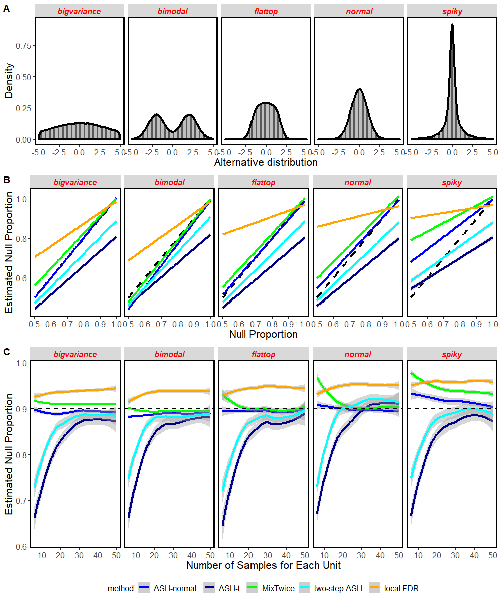
Figure 1: Errors in Estimation of $\pi_{0}$. Panel A shows distributions used for $g_{{\rm alt}}(\theta)$. Panel B shows the estimation of null proportion $\pi_{0}$ in case of equal samples in each group of 10. Methods are distinguished by color, where we report average parameter estimates from 500 simulated data sets.The identity line (dashed) indicates no bias. ASH-normal is an oracle case in which $\sigma_{i}^{2}=1$ is provided to the algorithm. Panel C shows error estimation as the number of observations grows, in $\pi_{0}=0.9$.

We are interested in the performance of MixTwice in scenarios reflecting what might be expected to occur in practice and have performed numerical experiments involving different generative distributions of both effects ($g$) and variances ($h$). Noting the special role of the null value, $\theta=0$, our experiments involve mixtures $g(\theta)=\pi_{0}\delta_{0}+(1-\pi_{0})g_{{\rm alt}}(\theta)$, where $\pi_{0}=\mathbb{P}(\theta_{i}=0)$ and $g_{\rm alt}$ provides various ways to distribute mass away from zero. Following Stephens (2017) and Lu and Stephens (2019), we entertain different general shapes, including so-called big-variance, bi-modal, flattop, normal, and spiky. MixTwice accounts for explicit differences between sample and underlying standard errors, and mixes nonparametrically over these underlying standard errors. Our numerical experiments consider the simplest case in which the data generating $h$ is a point mass, a case involving a finite mixture of two values, and also a continuous case of inverse-Gamma-distributed parameters. Patterns in the error of estimation and the hypothesis testing error rates are very comparable across different choices of $h$, and so for simplicity here we report only experiments when this true $h$ is a point mass distribution at $\sigma=1$. Figures 1 and 2 summarize, respectively, properties of estimation accuracy and testing error rates. Experiments are based on Gaussian samples, $m=1000$ peptides, and various sample size settings for the two-group comparison.

If a method tends to overestimate $\pi_{0}$, then power may be reduced; in case of underestimation the FDR may be inflated. Figure 1, Panel B, focuses on the estimation of this marginal null frequency for one choice of sample size, namely $n=10$ observations per group. In each setting of $g$ (column), 500 data sets are generated, each drawn after its own $\pi_{0}$ value was uniformly drawn in $[0.5,1]$. All methods respond appropriately to changes in $\pi_{0}$, though they exhibit different biases; MixTwice tracks the identity line (no bias) case closely in all scenarios except the challenging spiky case of $g_{\rm alt}$. By contrast locFDR is conservatively biased, tending to over-estimate $\pi_{0}$ in most cases. Our experiments include an oracle case, namely ASH$-$normal, which takes the true value $\sigma_{i}^{2}=1$ as known. This numerical control helps us gauge the magnitude of statistical errors induced by estimation error of the variance profile.

Figure 1, Panel C, amplifies one case from the second row, when $\pi_{0}=0.9$, and shows how estimation error drops as the sample size per peptide grows. Most methods display a level of convergence in this setting, with MixTwice performing relatively well especially at low sample sizes. Going beyond the estimation of $\pi_{0}$, we compared methods by their 1-Wassertstein error in estimating the entire mixture distribution $g$; MixTwice showed relatively small error in this setting also (data not shown). Without parametric assumptions, $\pi_{0}$ is not identifiable and only a upper bound may be reliably estimated (Efron et al., 2001, Stephens, 2017).

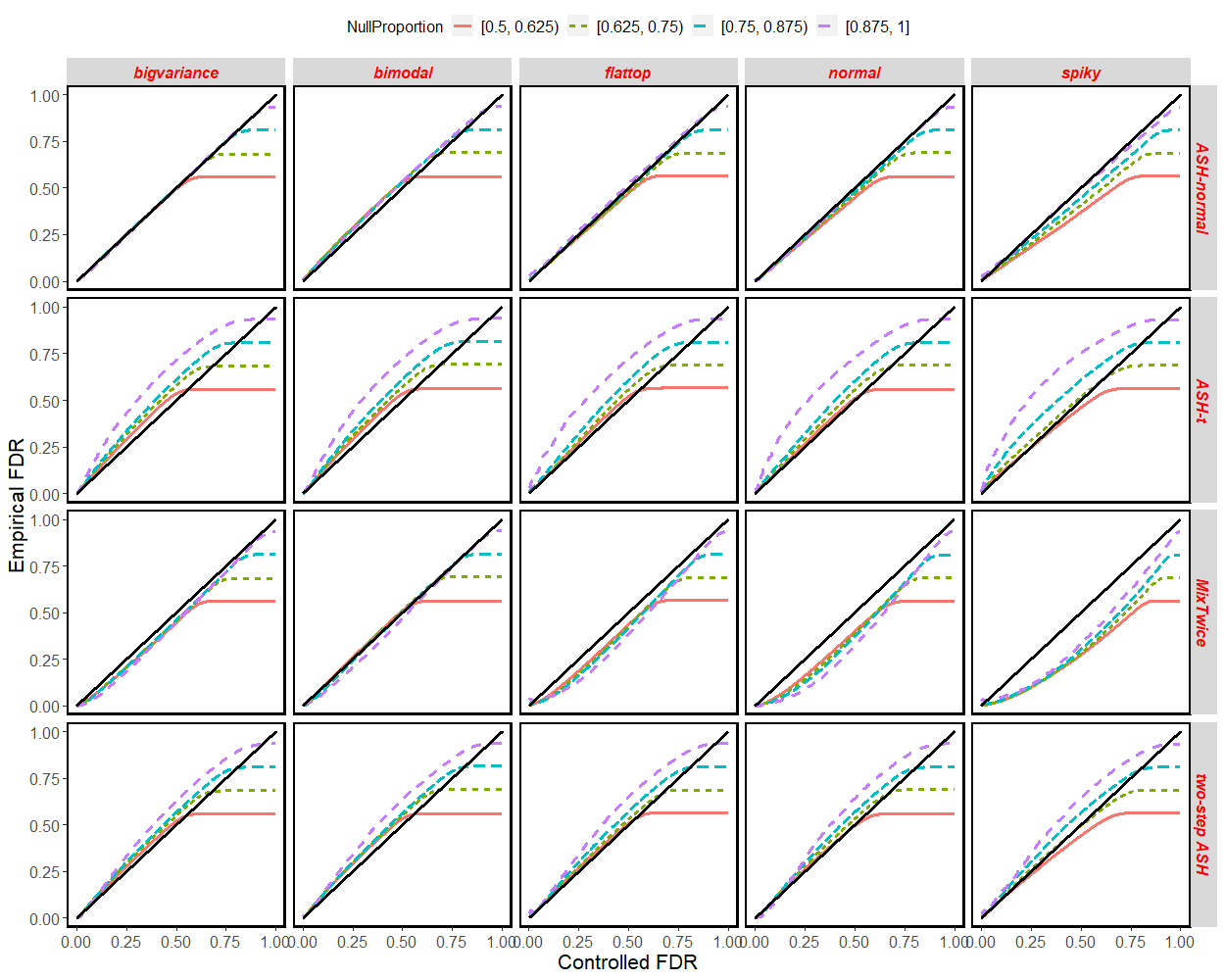
Figure 2: Synthetic data and FDR control: False discovery rates are shown by different methods (rows) under different alternative distributions $g_{{\rm alt}}(\theta)$ (columns). Empirical FDR (vertical) is the achieved error rate in the simulation; controlled FDR (horizontal) is the rate targeted by the methodology. Results with different $\pi_{0}$ are coded using different colors. A method tends to inflate FDR over the target level if its curve is greater than the identity line; it is conservative when its curve is dominated by the identity line.

Figure 2 confirms that most methods are controlling FDR as advertised. The empirical false discovery rate is plotted against the controlled rate; the latter is the nominal target FDR value where we threshold the lfdr’s; the former is what is evident from knowing the simulation states (in other terminology, it is the average, over simulated data sets, of the false discovery proportion). Colored lines are used to distinguish different levels of $\pi_{0}$, when the signal is dense (with a lower null proportion $\pi_{0}$) or when the signal is sparse (with a higher null proportion $\pi_{0}$). Recall we simulated independent data sets each governed by a randomly chosen $\pi_{0}$ from $[0.5,1]$. In order to visualize the results, we stratified data sets into four groups and averaged internally: $0.5\leq\pi_{0}\leq 0.625$, $0.625\leq\pi_{0}\leq 0.75$, $0.75\leq\pi_{0}\leq 0.875$, $0.875\leq\pi_{0}\leq 1$. The FDR inflation by ASH-t at high $\pi_{0}$ is evident in this simulation.

4 Empirical studies

4.1 Antibodies in rheumatoid arthritis

Rheumatoid arthritis (RA) is a chronic autoimmune disease characterized by inflammation and pain, primarily in the joints. RA patients produce autoantibodies against many different "self" proteins. Most famously, they generate antibodies against proteins in which arginine amino acids have been post-translationally modified to citrullines (Schellekens et al., 1998) as well as antibodies that bind to antibodies, called rheumatoid factor (RF) (Waaler, 1940). Both autoantibody types appear to be pathogenic (Sokolove et al., 2014) and both are used diagnostically (Aletaha et al., 2010), the former detected by the anti-cyclic citrullinated peptide (CCP) test. Most RA patients make both autoantibody types (CCP+RF+ RA), but some have only one type like in CCP+RF- RA. Little is known about why CCP+RF+ versus CCP+RF- RA develops. However, a better understanding of the autoantibody repertoires in each RA subset could provide insights, a task for which peptide arrays are perfect.

The custom high-density peptide array reported in Zheng et al. (2020) probed 172,828 distinct 12 amino acid length peptides derived from 122 human proteins suspected to be involved in RA, including peptides in which all arginines were replaced by citrullines. We reconsider here two distinct comparisons from that study, namely the comparison between CCP+RF- RA patients and controls, and a second comparison between CCP+RF+ RA patients and controls, in which differential signals are much stronger. Both comparisons have 12 subjects in each group. To assess reproducibility, we take advantage of a second peptide array data set derived from an independent set of 8 controls and 8 CCP+RF+ RA patients.

4.2 CCP+RF- RA: weak signals

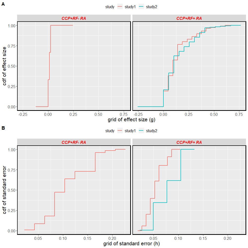
Figure 3: Estimated mixing distributions: For both effect distribution $g$ (Panel A) and squared-standard-error distribution $h$ (Panel B), shown are the maximum likelihood estimated mixing distributions as cumulative distribution functions (cdfs) in double natural log scale. The CCP+RF- RA example is shown on the left and the two CCP+RF+ RA examples are on the right.

We applied MixTwice to fit the shape-constrained mixture model of Section 2. Fitted mixing distributions are visualized in Figure 3 and provide a measure of the magnitude of changes in mean antibody levels as well as the magnitude of sampling variation. For example, the effect-size distribution estimates no probability for effects larger than 0.037. Also, the median standard error is 0.10 (squared standard error 0.01), which is large compared to the probable effect sizes.

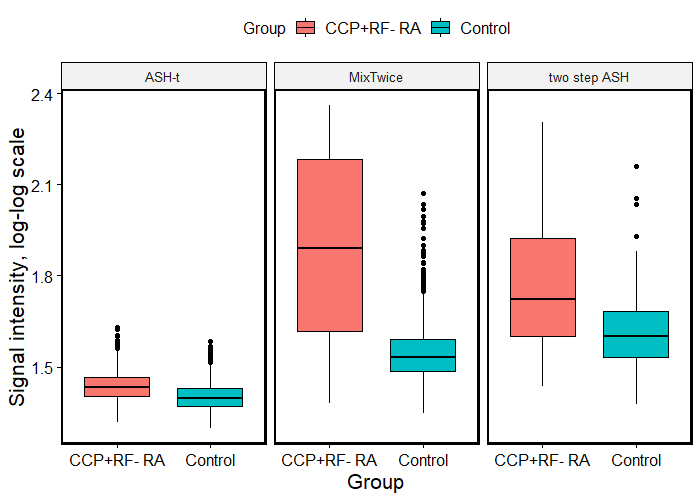
Figure 4: Signal intensity of differentially abundant peptides: Boxplots show averaged signal values on double natural log scale (both CCP+RF- RA and control subjects) for peptides found by ASH-t (76 peptides), MixTwice (44 peptides), and two-step ASH (11 peptides) all discovered at 10% FDR.

In Section 1 we presented summary counts of peptides identified at 10% FDR that exhibit differential binding between CCP+RF- RA patients and non-RA controls. MixTwice, ASH-t, and two-step ASH distinguish themselves in being the only methods among many standard large-scale tools to populate non-empty lists of discovered peptides at that FDR level. Recognizing that the magnitude of signal intensities on the peptide array is an important aspect of downstream analysis, Figure 4 shows a summary of the identified peptides by various methods. Notably, MixTwice and two-step ASH detect peptides in this case with higher average signal intensity than ASH-t; these may correspond to higher antibody abundance or affinity and potentially easier validation. ASH-t tends to select peptides with low standard errors, even when the estimated effects are very low.

Interestingly, the 44 peptides found by MixTwice have a strong pattern in their peptide sequences: all are citrulline ($B$)-containing peptides (which would be predicted for CCP+ RA patients) and contain citrulline next to glycine ($B$-$G$ or $G$-$B$), as shown in the motif in Figure 5. Binding of antigens in which citrulline is next to glycine is consistent with a growing body of literature on the reactivity of anti-citrullinated protein antibodies in RA (e.g., Burkhardt et al., 2002, Szarka et al., 2018, Steen et al., 2019, Zheng et al., 2020).

As a further negative control calculation, we applied MixTwice to each of 500 permuted data sets obtained by fixing the peptide data and randomly shuffling the 24 subject labels (12 control, 12 CCP+RF- RA). In 493 cases, the 10% FDR list is empty; 6 cases find a single peptide and one case finds 2 peptides at this threshold.

Among a number of large-scale testing methods applied to the CCP+RF- RA example, MixTwice identifies a comparatively large number of statistically significant peptides. By contrast to other methods, these peptides contain patterns in their amino acid sequences consistent with emerging evidence on this disease, and they correspond to relatively high fluorescence intensity measurements. Together, these observations provide some assurance that the MixTwice findings are not artifacts.

4.3 CCP+RF+ RA: strong signals

One of the findings from Zheng et al. (2020) concerns the extensive antibody-profile differences between RA patients who are positive for both biomarkers (CCP+RF+) and control subjects. Statistically, it represents an interesting non-sparse, large-scale testing situation, and the immunological mechanisms driving this remain only partially understood. To check the reproducibility of peptide-array findings, a new experiment was performed using the same procedures and 172,828 peptide array to detect IgG binding as in Zheng et al. (2020), but with serum samples from 16 different subjects: 8 CCP+RF+ RA and 8 controls. CCP+RF+ RA and control subjects were similar in regards to age, sex, race, ethnicity, and overall health. Preprocessing followed the same protocol and provided a data set (study 2) for us to look at reproducibility of large-scale hypothesis testing methods.

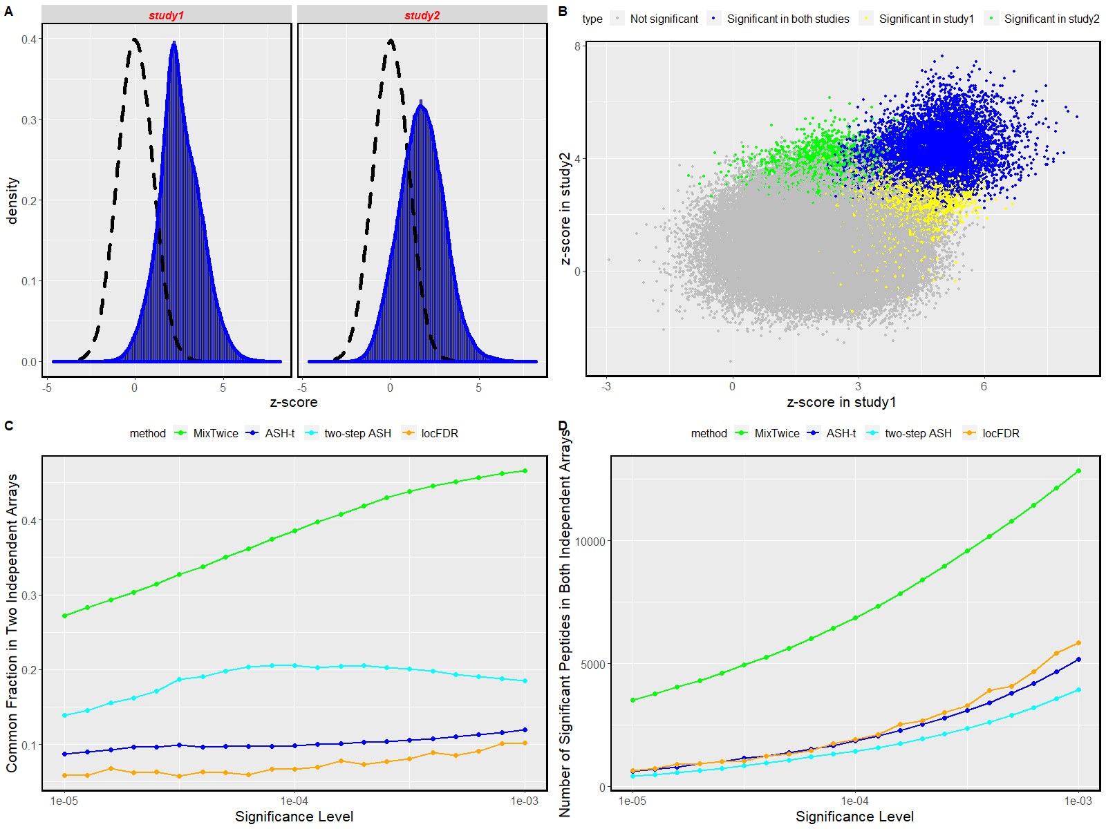
Figure 6: Reproducibility comparison. Panel A shows empirical z-score distributions for CCP+RF+ RA vs control at 172,828 peptides in two independent studies. The scatterplot in Panel B highlights peptides identified uniquely at 0.1% FDR by MixTwice in either study (yellow, green) and those reproducibly found in both studies (blue). Metrics in Panels C and D compare performance of MixTwice as a function of FDR threshold.

Z-score histograms in Figure 6, Panel A, show that both studies reveal extensive increased antibody binding in the CCP+RF+ RA group. The scatterplot in Panel B reveals concordance between the studies on this z-score metric. The color-coding highlights discovered peptides at the 0.1% FDR method by MixTwice, both uniquely in one study (green or yellow) and reproducibly in both studies (blue). Of course MixTwice uses more information than is in the z-score summary, but the scatterplot provides a convenient visualization. The lower panels in Figure 6 compare reproducibility statistics of different testing methods at various FDR thresholds. Denoting by $\mathcal{L}_{j}(\alpha)$ the list of significant peptides in study $j$ and FDR level $\alpha$, we have $|\mathcal{L}_{1}(\alpha)\cap\mathcal{L}_{2}(\alpha))|$ as the number of peptides identified in both studies (Panel D) and $\frac{|\mathcal{L}_{1}(\alpha)\cap\mathcal{L}_{2}(\alpha))|}{|\mathcal{L}_{1}(\alpha)\cup\mathcal{L}_{2}(\alpha))|}$ as the common fraction (Panel C). By connecting separate, independent studies of the same group difference, these statistics measure the reproducibility of various large-scale testing methods. MixTwice shows substantially better reproducibility than other testing methods, such as ASH-t, two-step ASH, and locFDR in this example.

5 Discussion

High-throughput biomedical experiments, such as those involving peptide arrays and immunological studies, continue to provide challenging problems for large-scale hypothesis testing. Readily applied techniques, such as $q-$value, locFDR, IHW, and ASH are often very effective at reporting lists of testing units (peptides) showing statistically significant effects at a targeted false discovery rate. In the case of high-density peptide arrays, we find several examples where these tools are deficient. One issue is the number of testing units, which is an order of magnitude larger than what is seen in transcript studies, for example. In the CCP+RF- RA comparison, most existing tools exhibit low power, which may stem in part from when they intervene in the data analysis. Methods that intervene earlier have access to more information and thereby may gain some advantage. The risk to intervening early is that more assumptions may be required to deliver relevant testing statistics (e.g., lfdr, lsdr). We rely on external validation, such as on sequence properties of the identified peptides, to assess practical utility. The CCP+RF+ RA example showcases a situation where power is high by all methods, and the differences boil down to how testing units are prioritized. The proposed MixTwice procedure shows impressive reproducibility in this case.

Structurally, MixTwice is similar to the ASH method for large-scale testing: it aims to estimate a mixing distribution of effects in an empirical Bayesian formulation. It adopts ASH’s nonparametric, shape-constrained model for effects, but deviates from that approach by incorporating a second mixing layer over underlying effect-variance parameters. A number of methodological issues deserve further study. For example, MixTwice treats the sampling model of squared standard errors as chi-square on a design-based degrees of freedom, which is rooted in a normal-data model. We expect that suitable transformation of the original data will make this treatment reasonable; for example, Zheng et al. (2020) proposed a double-log transform to stabilize variance. An interesting alternative is to use a bootstrap scheme to assess the sampling distributions directly, in order to thereby estimate the degrees of freedom that would be justified asymptotically for non-normal cases.

There are computational issues that warrant further investigation. The objective function (2) may not be convex in the pair of arguments $(g,h)$. Numerical experiments indicate good performance of the augmented Lagrangian optimization approach in a range of scenarios, though alternative approaches may have benefits. For example, the conditional optimizations of $g$ given $h$ or $h$ given $g$ are both convex, though attempts so far to leverage this have been less computationally efficient than the augmented Lagrangian method. Related to this are questions of grid sizes $K$ and $L$, which have to balance fidelity to the data and computational efficiency.

Though our presentation has focused on the classical two-group comparison problem, it should be evident that the core methodology is not restricted to this case. Estimated effects $x_{i}$, for example, could arise from a contrast of interest after adjusting for blocking variables or other covariates. These will be useful to consider as we expect them to emerge in experiments that further investigate mechanisms of immune-system disregulation.

Finally, we point out that other forms of information may be usefully integrated with the testing methodology. Peptides tile proteins, though we have treated them as anonymous testing units. More sophisticated peptide prioritization could leverage amino-acid structure, protein content, or other features of the immunological context.

Figure 5: Motif logo for significant peptides in CCP+RF- RA: Consensus sequences were generated using online software MEME Suite (Bailey et al., 2009) and the significant peptides from the different methods: ASH-t (left), MixTwice (middle) and two-step ASH (right). Each position of the motif logo represents the empirical distribution of amino acids at that site, with size proportional to frequency. $B$ found in the middle and right panels is citrulline, a post-transitionally modified arginine. The overall height of each stack is an information measure (bits) related to the concentration of the empirical distribution on its support.

Supplementary Material

Gradient and Hessian of optimization objective

We derive the gradient and Hessian of the log-likelihood equation, $l(g,h)$. Recall the definition of $l(g,h)$:

$$l(g,h) = \sum_{i=1}^{m}\log p(x_{i},s_{i}^{2}|g,h)$$

$$p(x_{i},s_{i}^{2}|g,h) = \sum_{k}\sum_{l}g_{k}h_{l}\,\frac{1}{\sqrt{b_{l}}}\phi\left(\frac{x_{i}-a_{k}}{\sqrt{b_{l}}}\right)\,\frac{\nu}{b_{l}}\chi_{2,\nu}\left(\frac{\nu s_{i}^{2}}{b_{l}}\right).$$

To simplify notation we use $c_{i,k,l}$ to denote the prior, mixture density of sample $i$ on the grid $a_{k},b_{l}$, and we let $d_{i}$ denote the observation density:

$$c_{i,k,l} := \frac{1}{\sqrt{b_{l}}}\phi\left(\frac{x_{i}-a_{k}}{\sqrt{b_{l}}}\right)\,\frac{\nu}{b_{l}}\chi_{2,\nu}\left(\frac{\nu s_{i}^{2}}{b_{l}}\right)$$

$$d_{i} := p(x_{i},s_{i}^{2}|g,h)=\sum_{k}\sum_{l}g_{k}h_{l}\ c_{i,k,l}.$$

Consider the parameter vector $(g,h)$ of length $(2K+1)+L$, where the first $2K+1$ components are for the effect mixing probabilities, $g=(g_{k})$, and the remaining $L$ components are for variance mixing probabilities $h=(h_{l})$. The quantities $c_{i,k,l}$ depend on the data, the support points but not the probabilities $g$ and $h$.

Constraints are critical to the optimization; of course all elements of $g$ and $h$ must be positive and sum to unity. We also impose a unimodality constraint on $g$. But in deploying the augmented Lagrangian method, these constraints act on the differentiable function $l(g,h)$, which we consider initially as varying freely over $2K+L+1$ Euclidean space. The gradient of $l(g,h)$ is a column vector of length $(2K+1)+L$ with the following format:

$$\nabla l(g,h) = \left(\left(\frac{\partial l(g,h)}{\partial g}\right)^{\prime},\left(\frac{\partial l(g,h)}{\partial h}\right)^{\prime}\right)^{\prime}$$

where each component has the explicit form:

$$\frac{\partial l(g,h)}{\partial g_{k}} = \sum_{i=1}^{m}\frac{1}{d_{i}}\sum_{l}h_{l}\ c_{i,k,l}$$

$$\frac{\partial l(g,h)}{\partial h_{l}} = \sum_{i=1}^{m}\frac{1}{d_{i}}\sum_{k}g_{k}\ c_{i,k,l}.$$

The Hessian of $l(g,h)$ is a $(2K+1)+L$ by $(2K+1)+L$ matrix:

$$\nabla^{2}l(g,h)=\begin{pmatrix}A&B\\ B^{\prime}&C\end{pmatrix}$$

where matrix $A$ ($2K+1$ by $2K+1$) contains second derivative with respect to $g$, matrix $C$ ($L$ by $L$) contains second derivative with respect to $h$ and matrix $B$ ($2K+1$ by $L$) contains second derivative with respect to $g$ and $h$.

For entries of matrix $A$:

$$\frac{\partial^{2}l(g,h)}{\partial g_{k}^{2}} = -\sum_{i=1}^{m}\frac{1}{d_{i}^{2}}\left(\sum_{l}h_{l}\ c_{i,k,l}\right)^{2}$$

$$\frac{\partial^{2}l(g,h)}{\partial g_{k_{1}}\partial g_{k_{2}}} = -\sum_{i=1}^{m}\frac{1}{d_{i}^{2}}\left(\sum_{l}h_{l}\ c_{i,k_{1},l}\right)\left(\sum_{l}h_{l}\ c_{i,k_{2},l}\right).$$

For entries of matrix $C$:

$$\frac{\partial^{2}l(g,h)}{\partial h_{l}^{2}} = -\sum_{i=1}^{m}\frac{1}{d_{i}^{2}}\left(\sum_{k}g_{k}\ c_{i,k,l}\right)^{2}$$

$$\frac{\partial^{2}l(g,h)}{\partial h_{l_{1}}\partial h_{l_{2}}} = -\sum_{i=1}^{m}\frac{1}{d_{i}^{2}}\left(\sum_{k}g_{k}\ c_{i,k,l_{1}}\right)\left(\sum_{k}g_{k}\ c_{k,l_{2}}\right).$$

For entries of matrix $B$:

$$\frac{\partial^{2}l(g,h)}{\partial g_{k}\partial h_{l}} = \sum_{i=1}^{m}\frac{1}{d_{i}^{2}}\left(c_{i,k,l}\ d_{i}-\sum_{l}h_{l}\ c_{i,k,l}\sum_{k}g_{k}\ c_{i,k,l}\right).$$

Random subsampling

The optimization to compute $\hat{g}$ and $\hat{h}$ becomes computationally challenging as the number of testing units increases. MixTwice provides an option for users to use a randomly-selected subset of testing units to obtain the fitted distributions. Here we illustrate the compute-time improvements associated with relatively little degradation in the quality of the estimates.

We use the CCP+RF+ RA example to illustrate the random subsampling properties in terms of estimation error and computational benefit. Relative to the estimate obtained from half the units, we evaluate the discrepancy in distribution estimation and the user’s CPU time (with Inter(R) Core(TM) i5-7400HQ CPU processor) when the prop, the proportion of testing units used to fit the distribution, changes. We use $1$-Wasserstein distance between two cumulative distribution functions as the metric to evaluate the discrepancy from the case when $\verb+prop+=0.5$ as benchmark.

Figure 7 summaries the result. Panel A highlights the estimation of $\hat{g},\hat{h}$ when $\verb+prop+=0.5,0.1,0.01$ where the estimations are quite similar. Panel B shows how the discrepancy decreases when the proportion of testing units used to fit the distribution increases. Note that even when $\verb+prop+=0.01$, the discrepancy is quite small (error in $\hat{g}$ less than 0.02 and error in $\hat{h}$ only $10^{-}4$). Panel C shows the computational benefits.

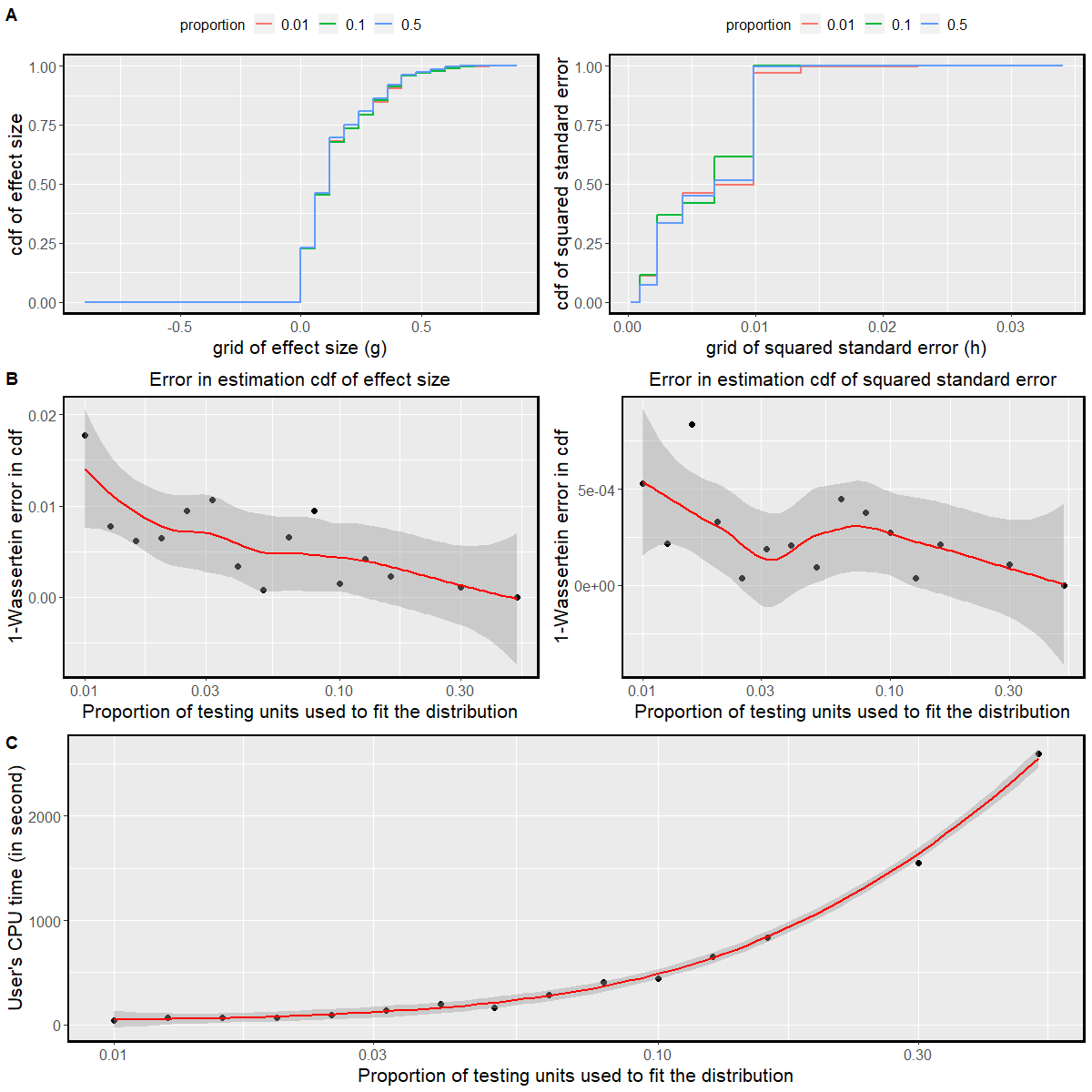
Figure 7: How does random subsampling influence estimation accuracy and computational efficiency? Panel A shows the estimation in $\hat{g},\hat{h}$ when various proportions of the units are used for estimation. Panel B shows the 1-Wasserstein discrepancy (between estimate at that proportion and estimate from half the units) as a function of subsampling proportion. Panel C shows the corresponding CPU time.

References

- Aletaha et al. (2010) D. Aletaha, T. Neogi, A. J. Silman, J. Funovits, D. T. Felson, C. O. Bingham III, N. S. Birnbaum, G. R. Burmester, V. P. Bykerk, M. D. Cohen, et al. 2010 rheumatoid arthritis classification criteria: an american college of rheumatology/european league against rheumatism collaborative initiative. Arthritis & rheumatism, 62(9):2569–2581, 2010.
- Bailey et al. (2017) A. L. Bailey, C. R. Buechler, D. R. Matson, E. J. Peterson, K. G. Brunner, M. S. Mohns, M. Breitbach, L. M. Stewart, A. J. Ericsen, C. M. Newman, et al. Pegivirus avoids immune recognition but does not attenuate acute-phase disease in a macaque model of hiv infection. PLoS pathogens, 13(10):e1006692, 2017.
- Bailey et al. (2020) J. A. Bailey, A. A. Berry, M. A. Travassos, A. Ouattara, S. Boudova, E. Y. Dotsey, A. Pike, C. G. Jacob, M. Adams, J. C. Tan, et al. Microarray analyses reveal strain-specific antibody responses to plasmodium falciparum apical membrane antigen 1 variants following natural infection and vaccination. Scientific reports, 10(1):1–12, 2020.
- Bailey et al. (2009) T. L. Bailey, M. Boden, F. A. Buske, M. Frith, C. E. Grant, L. Clementi, J. Ren, W. W. Li, and W. S. Noble. Meme suite: tools for motif discovery and searching. Nucleic acids research, 37(suppl_2):W202–W208, 2009.
- Benjamini and Hochberg (1995) Y. Benjamini and Y. Hochberg. Controlling the false discovery rate: a practical and powerful approach to multiple testing. Journal of the Royal statistical society: series B (Methodological), 57(1):289–300, 1995.
- Bourgon et al. (2010) R. Bourgon, R. Gentleman, and W. Huber. Independent filtering increases detection power for high-throughput experiments. Proceedings of the National Academy of Sciences, 107(21):9546–9551, 2010.
- Burkhardt et al. (2002) H. Burkhardt, T. Koller, Å. Engström, K. S. Nandakumar, J. Turnay, H. G. Kraetsch, J. R. Kalden, and R. Holmdahl. Epitope-specific recognition of type ii collagen by rheumatoid arthritis antibodies is shared with recognition by antibodies that are arthritogenic in collagen-induced arthritis in the mouse. Arthritis & Rheumatism, 46(9):2339–2348, 2002.
- Efron (2012) B. Efron. Large-scale inference: empirical Bayes methods for estimation, testing, and prediction, volume 1. Cambridge University Press, 2012.
- Efron et al. (2001) B. Efron, R. Tibshirani, J. D. Storey, and V. Tusher. Empirical bayes analysis of a microarray experiment. Journal of the American statistical association, 96(456):1151–1160, 2001.
- Hoefges et al. (2020) A. Hoefges, A. K. Erbe-Gurel, S. J. McIlwain, A. S. Melby, A. Xu, N. Mathers, A. L. Rakhmilevich, J. A. Hank, C. Baniel, R. Pinapati, et al. Thousands of new antigens are recognized in mice via endogenous antibodies after being cured of a b78 melanoma via immunotherapy, 2020.
- Ignatiadis et al. (2016) N. Ignatiadis, B. Klaus, J. B. Zaugg, and W. Huber. Data-driven hypothesis weighting increases detection power in genome-scale multiple testing. Nature methods, 13(7):577–580, 2016.
- Korthauer et al. (2019) K. Korthauer, P. K. Kimes, C. Duvallet, A. Reyes, A. Subramanian, M. Teng, C. Shukla, E. J. Alm, and S. C. Hicks. A practical guide to methods controlling false discoveries in computational biology. Genome biology, 20(1):1–21, 2019.
- Lu and Stephens (2019) M. Lu and M. Stephens. Empirical bayes estimation of normal means, accounting for uncertainty in estimated standard errors. arXiv preprint arXiv:1901.10679, 2019.
- Mishra et al. (2018) N. Mishra, A. Caciula, A. Price, R. Thakkar, J. Ng, L. V. Chauhan, K. Jain, X. Che, D. A. Espinosa, M. M. Cruz, et al. Diagnosis of zika virus infection by peptide array and enzyme-linked immunosorbent assay. MBio, 9(2), 2018.
- Newton et al. (2006) M. Newton, P. Wang, and C. Kendziorski. Hierarchical mixture models for expression profiles. In Bayesian inference for gene expression and proteomics, chapter 2, pages 40–52. Cambridge University Press New York, 2006.
- O’Neill (2014) B. O’Neill. Some useful moment results in sampling problems. The American Statistician, 68(4):282–296, 2014.
- Schellekens et al. (1998) G. A. Schellekens, B. De Jong, F. Van den Hoogen, L. Van de Putte, W. J. van Venrooij, et al. Citrulline is an essential constituent of antigenic determinants recognized by rheumatoid arthritis-specific autoantibodies. The Journal of clinical investigation, 101(1):273–281, 1998.
- Sokolove et al. (2014) J. Sokolove, D. S. Johnson, L. J. Lahey, C. A. Wagner, D. Cheng, G. M. Thiele, K. Michaud, H. Sayles, A. M. Reimold, L. Caplan, et al. Rheumatoid factor as a potentiator of anti–citrullinated protein antibody–mediated inflammation in rheumatoid arthritis. Arthritis & rheumatology, 66(4):813–821, 2014.
- Steen et al. (2019) J. Steen, B. Forsström, P. Sahlström, V. Odowd, L. Israelsson, A. Krishnamurthy, S. Badreh, L. Mathsson Alm, J. Compson, D. Ramsköld, et al. Recognition of amino acid motifs, rather than specific proteins, by human plasma cell–derived monoclonal antibodies to posttranslationally modified proteins in rheumatoid arthritis. Arthritis & Rheumatology, 71(2):196–209, 2019.
- Stephens (2017) M. Stephens. False discovery rates: a new deal. Biostatistics, 18(2):275–294, 2017.
- Storey et al. (2003) J. D. Storey et al. The positive false discovery rate: a bayesian interpretation and the q-value. The Annals of Statistics, 31(6):2013–2035, 2003.
- Strimmer (2008) K. Strimmer. fdrtool: a versatile r package for estimating local and tail area-based false discovery rates. Bioinformatics, 24(12):1461–1462, 2008.
- Szarka et al. (2018) E. Szarka, P. Aradi, K. Huber, J. Pozsgay, L. Végh, A. Magyar, G. Gyulai, G. Nagy, B. Rojkovich, É. Kiss, et al. Affinity purification and comparative biosensor analysis of citrulline-peptide-specific antibodies in rheumatoid arthritis. International Journal of Molecular Sciences, 19(1):326, 2018.
- Tokarz et al. (2020) R. Tokarz, T. Tagliafierro, A. Caciula, N. Mishra, R. Thakkar, L. V. Chauhan, S. Sameroff, S. Delaney, G. P. Wormser, A. Marques, et al. Identification of immunoreactive linear epitopes of borrelia miyamotoi. Ticks and tick-borne diseases, 11(1):101314, 2020.
- Varadhan (2015) R. Varadhan. alabama: Constrained Nonlinear Optimization, 2015. URL https://CRAN.R-project.org/package=alabama. R package version 2015.3-1.
- Waaler (1940) E. Waaler. On the occurrence of a factor in human serum activating the specific agglutination of sheep blood corpuscles. Acta Pathologica Microbiologica Scandinavica, 17(2):172–188, 1940.
- Yan et al. (2019) Y. Yan, N. Sun, H. Wang, M. Kobayashi, J. J. Ladd, J. P. Long, K. C. Lo, J. Patel, E. Sullivan, T. Albert, et al. Whole genome–derived tiled peptide arrays detect prediagnostic autoantibody signatures in non–small-cell lung cancer. Cancer research, 79(7):1549–1557, 2019.
- Zheng et al. (2020) Z. Zheng, A. M. Mergaert, L. M. Fahmy, M. Bawadekar, C. L. Holmes, I. M. Ong, A. J. Bridges, M. A. Newton, and M. A. Shelef. Disordered antigens and epitope overlap between anti–citrullinated protein antibodies and rheumatoid factor in rheumatoid arthritis. Arthritis & Rheumatology, 72(2):262–272, 2020.