¹Mathematics Section, EOT, tv42022@tvdsb.ca, terrymoschandreou@yahoo.com, Thames Valley District School Board, London Ontario, Canada

Periodic Navier Stokes Equations: Wave Equation Reduction and Existence of Non-Smooth Solutions for Non-Constant Vorticity

Copyright ©2021 by authors, all rights reserved. Authors agree that this article remains permanently
open access under the terms of the Creative Commons Attribution License 4.0 International License

Abstract   A rigorous proof of no finite time blowup of the 3D Incompressible Navier Stokes equations in $\mathbb{R}^{3}/\mathbb{Z}^{3}$ has been shown by corresponding author of the present work [1]. Smooth solutions for the $z-$component momentum equation $u_{z}$ assuming the $x$ and $y$ component equations have vortex smooth solutions have been proven to exist, however the Clay Institute Millennium problem on the Navier Stokes equations was not proven for a general enough vorticity form and [1], [3] and references therein do not prove this as previously thought. The idea was to show that Geometric Algebra can be applied to all three momentum equations by adding any two of the three equations and thus combinatorially producing either $u_{x}$, $u_{y}$ or $u_{z}$ as smooth solutions at a time. It was shown that using the Gagliardo-Nirenberg and Prékopa-Leindler inequalities together with Debreu’s theorem and some auxiliary theorems proven in [1] that there is no finite time blowup for 3D Navier Stokes equations for a constant vorticity in the $z$ direction. In part I of the present work it is shown that using Hardy’s inequality for $u^{2}_{z}$ term in the Navier Stokes Equations that a resulting PDE emerges which can be coupled to auxiliary pde’s which give us wave equations in each of the three principal directions of flow. The present work is extended to all spatial directions of flow for the most general flow conditions. In Part II it is shown for the first time that the full system of 3D Incompressible Navier Stokes equations without the above mentioned coupling consists of non-smooth solutions. In particular if $u_{x}$, $u_{y}$ satisfy a non-constant $z$- vorticity for 3D vorticity $\vec{\omega}$, then higher order derivatives blowup in finite time but $u_{z}$ remains regular. So a counterexample of the Navier Stokes equations having smooth solutions is shown. A specific time dependent vorticity is also considered.

Keywords Millennium, Navier Stokes, Geometric Algebra, Gagliardo-Nirenberg, Prékopa-Leindler, Hardy Inequality, Debreu, Brouwer, Lusin, Lebesgue Integral, finite time blowup, Non-Smooth solutions

1 Introduction

The global regularity of the Navier-Stokes equations remains to be an outstanding unsolved problem in fluid mechanics. The Clay Institute is offering a significant prize for those who are successful in solving either one of four proposed problems, that is either a periodic or non-periodic regular or finite time blowup problem for the full 3D Navier Stokes equations, See[1] and references therein. A turbulent flow field is characterized by rapid fluctuations. This flow is too complicated to be known in full detail. There are various reasons for the occurrence of turbulence. For example instabilities can occur due to viscosity. Viscosity converts kinetic energy into heat thus resulting in turbulence. Shearing flows with high Reynold’s numbers can result in turbulence. The question of whether turbulence is created deterministically or stochastically for fluid flows is still an open problem. In experiments, turbulence is often created deterministically. For example, wind tunnels are designed with low background disturbances and excitation sources in boundary layers that do cause transition from laminar to turbulent flow. Work in the area of Spatio-Temporal Wavefronts (STWF) has been carried out in [2] and references therein and identify the unit process of transition to be the STWF. Also, here it is stated that "once a STWF is created by a linear mechanism, subsequent linear growth is followed by non-linear effects, which cause STWF’s to display a regeneration mechanism. Small areas of turbulence result which join together to develop into fully developed turbulent flow. In the present work, specific auxiliary equations are introduced which differentially relate $u_{z}$ to $u_{x}$ and $u_{z}$ to $u_{y}$ velocities in the momentum equations. These equations are fourth order in time $t$. Specifically Eq.(5) in this work(also found in the less general case of $u_{x}$ and $u_{y}$ not variating wrt to $z$ in [1], [3] and [4]), are now dealt for extended problem such that the $\Omega_{5}=\nabla u^{2}_{z}\cdot\frac{\partial\vec{b}}{\partial t}$ term is considered for $\vec{b}=\frac{1}{\delta}(u_{x}\vec{i}+u_{y}\vec{j}+\epsilon u_{z}\vec{k})$ with $u_{x}$,$u_{y}$ and $u_{z}$ variating in $x$, $y$ and $z$ and $\epsilon>0$. Here I use the already proven fact that $u_{z}$ is smooth [1](see references therein). The idea is to show that Geometric Algebra can be applied to all three momentum equations by adding any two of the three equations and thus combinatorially producing either $u_{x}$, $u_{y}$ or $u_{z}$ as smooth solutions at a time. Having guaranteed a smooth function it can be now shown that by using the Hardy Inequality for $u^{2}_{z}$ as shown in Appendix that a resulting PDE occurs by a limiting "sandwich analysis" which ensures that the norm is in fact zero.-(See [1], [3] and [4]), where it is shown that the negative of $L_{2}$ norm of the gradient of $\vec{u}$ is greater than or equal to zero due to division by the volume of a cube which tends to infinity. See analysis section of this paper)). In part I of the present work it is shown that using Hardy’s inequality for $u^{2}_{z}$ term in the Navier Stokes Equations that a resulting PDE emerges which can be coupled to auxiliary pde’s which give us wave equations in each of the three principal directions of flow. The auxiliary equations are listed in the Appendix of this paper in a Maple programming code which can be used to show that the full 3D Navier Stokes and coupling equations can be interpreted as a series of wave equations in $\mathbb{R}^{3}$. The physical interpretation is that due to friction between shear layers in a viscous fluid that waves are produced. The present work is extended to all spatial directions of flow for the most general flow conditions. See also recent work on wave solutions to the Riemann wave equations and the Landau-Ginsburg-Higgs equation in [5]. Very recently in 2019 an important work on the search for wave phenomena in the incompressible Navier Stokes Equations has been undertaken with a historical perspective of the author’s and others’ related work in [6]. Various types of waves in related papers are found there. Based on the work of Truesdell, the possibility emerged that "other" types of waves, not longitudinal, and singular surfaces could exist within a flow space and not violate the incompressibility constraint. See Truesdell’s work in [7]-[9]. In Part II it is shown for the first time that the full system of 3D Incompressible Navier Stokes equations without the above mentioned coupling consists of non-smooth solutions. In particular if $u_{x}$, $u_{y}$ satisfy a non-constant $x-y-z$- or time dependent vorticity for 3D vorticity $\vec{\omega}$, then a blowup in finite time is presented here. So a counterexample of the Navier Stokes equations possessing smooth solutions is shown. See also [10] and references therein for a finite time blowup but with solutions that have linear growth at infinity

1.1 Equations

The 3D incompressible unsteady Navier-Stokes Equations (NSEs) in Cartesian coordinates may be written in the form for the velocity field $\textbf{u}^{*}=u^{*i}\vec{\textbf{e}}_{i}\phantom{.},\phantom{.}u^{*i}=\{u^{*}_{x},u^{*}_{y},u^{*}_{z}\}$:

$$\rho\left(\frac{\partial}{\partial t^{*}}+u^{*j}\nabla_{*j}\right)u^{*}_{i}-\mu\nabla^{2}_{*}u^{*}_{i}+\nabla_{*i}P^{*}=\rho F^{*}_{i}$$ (1)

where $\rho$ is constant density, $\mu$ is dynamic viscosity, and $\textbf{F}^{*}=F^{*i}\vec{\textbf{e}}_{i}$ are body forces on the fluid. The components of the velocity vector, and pressure in $\textbf{u}=(u)^{i}\vec{\textbf{e}}_{i}$, $\textbf{P}=(P)^{i}\vec{\textbf{e}}_{i}$, coordinates $\textbf{x}_{i}$ and time $t$, are reparametrized according to the following form utilizing the non-dimensional quantity $\delta\in R$:

$$u^{*}_{i}=\frac{1}{\delta}u_{i}\phantom{.},\phantom{.}P^{*}_{i}=\frac{1}{\delta^{2}}P_{i}\phantom{.},\phantom{.}x^{*}_{i}=\delta x_{i}\phantom{.},\phantom{.}t^{*}=\delta^{2}t$$ (2)

Along with Eq.(1), the continuity equation in Cartesian co-ordinates, is given in tensor index notation by:

$$\nabla^{i}u_{i}=0$$ (3)

1.2 Decomposition of NSEs

For Eqs.(1)-(3) the Dirichlet condition $\vec{u^{*}}(\vec{x^{*}},0)=\vec{\xi}(\vec{x^{*}})$ such that $\nabla\cdot\vec{\xi}=0$ describes the NSEs together with an incompressible initial condition. Considering periodic boundary conditions specified in the Millennium problem, defined on a cube subset $\Omega\subset\mathbb{R}^{3}$ with associated Lattice in $\mathbb{R}^{3}$ is the periodic BVP for the NSEs. In [3] and [4] a solution for Eqs.(1)-(3) exists in the form,

$${\bf{u}}=(u_{x},u_{y},u_{z})\mathrel{\mathop{\mathchar 58\relax}}\mathbb{R^{+}}\times\mathbb{R}^{3}/\mathbb{Z}^{3}\to\mathbb{R}^{3}$$ (4)

where $u_{z}$ in Eq.(4) satisfies the following integral equation,

2 The Existence of Spatio-Temporal Waves for the Navier-Stokes equations coupled to a set of Auxiliary Equations

An extension to the work done previously in [1], the following analysis shows the velocities $u_{x}$, $u_{y}$ and $u_{z}$ changing in the $z$ direction as well as the $x$ and $y$ directions,

$$\begin{matrix}\left({\delta}^{-1}-1\right)\left({\frac{\partial u_{z}}{\partial t}}\right)^{2}+{\frac{\mu\,\left({\frac{\partial u_{z}}{\partial t}}\right)\left({\frac{\partial^{2}u_{z}}{\partial{x}^{2}}}+{\frac{\partial^{2}u_{z}}{\partial{y}^{2}}}+{\frac{\partial^{2}u_{z}}{\partial{z}^{2}}}\right)}{\rho}\left(1-{\delta}^{-1}\right)}+\\ u^{2}_{z}{\frac{\partial^{2}u_{z}}{\partial z\partial t}}+\delta\,\left(\left({\it u_{x}}\right)^{2}+\left({\it u_{y}}\right)^{2}+\left({\it u_{z}}\right)^{2}\right)\times\\ \left(2\,\left({\frac{\partial u_{z}}{\partial x}}\right)^{2}+2u_{z}{\frac{\partial^{2}u_{z}}{\partial{x}^{2}}}+2\,\left({\frac{\partial u_{z}}{\partial y}}\right)^{2}+2\,{\it uz}{\frac{\partial^{2}u_{z}}{\partial{y}^{2}}}+2\,\left({\frac{\partial u_{z}}{\partial z}}\right)^{2}+2\,{\it uz}{\frac{\partial^{2}u_{z}}{\partial{z}^{2}}}\right)\\ \\ -{\frac{\mu\,\left({\it u_{z}}\right)^{2}\left({\frac{\partial^{3}u_{x}}{\partial{x}^{3}}}+{\frac{\partial^{3}u_{y}}{\partial{y}^{3}}}+{\frac{\partial^{3}u_{z}}{\partial{z}^{3}}}+{\frac{\partial^{3}u_{y}}{\partial{y}^{2}\partial x}}+{\frac{\partial^{3}u_{z}}{\partial{z}^{2}\partial x}}+{\frac{\partial^{3}u_{x}}{\partial y\partial{x}^{2}}}+{\frac{\partial^{3}u_{y}}{\partial{z}^{2}\partial y}}+{\frac{\partial^{3}u_{x}}{\partial z\partial{x}^{2}}}+{\frac{\partial^{3}u_{y}}{\partial z\partial{y}^{2}}}\right)}{\delta\,\rho}}\\ +{\frac{\left({\it u_{z}}\right)^{2}\left({\frac{\partial^{2}u_{z}}{\partial z\partial t}}+{\frac{\partial^{3}u_{z}}{\partial{z}^{3}}}\right)}{\delta}}+(\frac{1}{\delta}-1)\frac{1}{\rho}\frac{\partial u_{z}}{\partial t}\frac{\partial P}{\partial z}+\\ \iint_{S}\ \big{(}\frac{1}{\delta\rho}u^{2}_{z}\nabla_{xy}P+\vec{b}\frac{1}{\rho}u_{z}\frac{\partial P}{\partial z}\big{)}\cdot\vec{n}\ dS+\\ \delta^{2}\vec{F_{T}}\cdot\nabla u^{2}_{z}-\delta^{3}u_{z}\frac{\partial u_{z}}{\partial t}\frac{\partial u_{z}}{\partial z}F_{z}+\delta^{3}\vec{b}\cdot\nabla(u_{z}F_{z})-\\ \frac{1}{\mathinner{\!\left\lVert\vec{b}\right\rVert}}\int_{U}\mathinner{\!\left\lVert\frac{\partial u_{z}}{\partial t}\vec{b}\cdot\left(\vec{b}\otimes\nabla u_{z}\right)\right\rVert}dV=0\end{matrix}$$ (5)

$$\begin{matrix}P_{zz}=-{\it u_{z}}\left({\frac{\partial^{2}u_{z}}{\partial{x}^{2}}}+{\frac{\partial^{2}u_{z}}{\partial{y}^{2}}}+{\frac{\partial^{2}u_{z}}{\partial{z}^{2}}}\right)-{\it u_{z}}{\frac{\partial^{2}u_{z}}{\partial{x}^{2}}}-{\it u_{z}}{\frac{\partial^{2}u_{z}}{\partial{y}^{2}}}-\left({\frac{\partial u_{z}}{\partial z}}\right)^{2}-\\ {\it u_{z}}{\frac{\partial^{2}u_{z}}{\partial{z}^{2}}}+{\frac{\partial^{2}u_{z}}{\partial z\partial x}}+{\frac{\partial^{2}u_{z}}{\partial z\partial y}}-\delta\,{\it u_{x}}{\frac{\partial^{2}u_{z}}{\partial z\partial x}}-\delta\,{\it u_{y}}{\frac{\partial^{2}u_{z}}{\partial z\partial y}}-{\frac{\partial^{2}u_{z}}{\partial z\partial t}}-{\frac{\partial^{3}u_{z}}{\partial{z}^{3}}}\end{matrix}$$ (6)

Solve for $\frac{\partial P}{\partial z}$ in Eq.(5), differentiating wrt to $z$ and substituting and equating to Eq.(6), and setting $\vec{F_{T}}$ and $F_{z}$ to zero as in [4] results in a new PDE in $u_{z}$. The pressure terms integral is set equal to the integral of the tensor product term. It will become apparent why this is done as we will return here to complete the calculation for both pressure and $u_{z}$ velocity.

2.1 Extension to all spatial directions of flow

In the expression for $\Omega_{5}=\nabla u^{2}_{z}\cdot\frac{\partial\vec{b}}{\partial t}$ in Eq. (5) assuming that $\vec{b}$ is extended to $u_{x},u_{y}$ and $u_{z}$, that is,

$$\vec{b}=\frac{1}{\delta}u_{x}\vec{i}+\frac{1}{\delta}u_{y}\vec{j}+\frac{1}{\delta}u_{z}\vec{k}$$ (7)

where,

$$u_{z}\rightarrow\frac{u_{z}}{\eta}$$

for large $\eta$, then

$$\int_{\Omega}\nabla u^{2}_{z}\cdot\frac{\partial\vec{b}}{\partial t}dv=-\delta\Bigg{[}\int_{\Omega}\frac{\partial u^{2}_{z}}{\partial x}\left(u_{x}\frac{\partial u_{x}}{\partial x}+u_{y}\frac{\partial u_{y}}{\partial x}+u_{z}\frac{\partial u_{z}}{\partial x}\right)+$$

$$\frac{\partial u^{2}_{z}}{\partial y}\left(u_{x}\frac{\partial u_{x}}{\partial y}+u_{y}\frac{\partial u_{y}}{\partial y}+u_{z}\frac{\partial u_{z}}{\partial y}\right)+$$

$$\frac{\partial u^{2}_{z}}{\partial z}\left(u_{x}\frac{\partial u_{x}}{\partial z}+u_{y}\frac{\partial u_{y}}{\partial z}+u_{z}\frac{\partial u_{z}}{\partial z}\right)dv\Bigg{]}+\dots$$ (8)

In the entire paper $u_{z}$ denotes $u_{z}$ divided by $\eta$. In the limit we obtain the two dimensional Navier Stokes equations. See [3], Eq.(17) there. Thus by integration by parts,

$$\int_{\Omega}\nabla u^{2}_{z}\cdot\frac{\partial\vec{b}}{\partial t}dv=-\delta\int_{\Omega(y,z)}\frac{\partial u^{2}_{z}}{\partial x}\ \mathinner{\!\left\lVert\vec{u}\right\rVert}^{2}\mid_{\text{x-bdry}}dydz+$$

$$\delta\int_{\Omega}\frac{\partial^{2}u^{2}_{z}}{\partial x^{2}}\mathinner{\!\left\lVert\vec{u}\right\rVert}^{2}dxdydz-\delta\int_{\Omega(x,z)}\frac{\partial u^{2}_{z}}{\partial y}\ \mathinner{\!\left\lVert\vec{u}\right\rVert}^{2}\mid_{\text{y-bdry}}dxdz+$$

$$\delta\int_{\Omega}\frac{\partial^{2}u^{2}_{z}}{\partial y^{2}}\mathinner{\!\left\lVert\vec{u}\right\rVert}^{2}dydxdz-\delta\int_{\Omega(x,y)}\frac{\partial u^{2}_{z}}{\partial z}\ \mathinner{\!\left\lVert\vec{u}\right\rVert}^{2}\mid_{\text{z-bdry}}dxdy+$$

$$\delta\int_{\Omega}\frac{\partial^{2}u^{2}_{z}}{\partial z^{2}}\mathinner{\!\left\lVert\vec{u}\right\rVert}^{2}dzdxdy$$ (9)

and because $\mathinner{\!\left\lVert\vec{u}\right\rVert}$ is zero on the respective boundaries,

$$\int_{\Omega}\nabla u^{2}_{z}\cdot\frac{\partial\vec{b}}{\partial t}dv=\delta\int_{\Omega}\nabla^{2}u^{2}_{z}\ \mathinner{\!\left\lVert\vec{u}\right\rVert}^{2}dv$$ (10)

The next term in $\Omega_{5}$ is $-\frac{\mu}{\rho}\int_{\Omega}\nabla u^{2}_{z}\cdot\nabla^{2}\vec{b}dv$. All together including pressure term $P_{xx}+P_{yy}$ (see Eq (4) and Poisson’s equation in [3]), Integrating by parts gives,

$$\begin{matrix}\int_{\Omega}\nabla u^{2}_{z}\cdot\frac{\partial\vec{b}}{\partial t}dv=\delta\int_{\Omega}\nabla^{2}u^{2}_{z}\ \mathinner{\!\left\lVert\vec{u}\right\rVert}^{2}dv+\\ \frac{\mu}{\delta\rho}{\it u^{2}_{z}}\left({\frac{\partial^{3}u_{x}}{\partial{x}^{3}}}+{\frac{\partial^{3}u_{y}}{\partial{y}^{3}}}+{\frac{\partial^{3}u_{z}}{\partial{z}^{3}}}\right)+{\frac{\it u^{2}_{z}}{\delta}\left({\frac{\partial^{2}u_{z}}{\partial z\partial t}}+{\frac{\partial^{3}u_{z}}{\partial{z}^{3}}}\right)}\end{matrix}$$

Hence Eq.(5), Eq.(12) become,

$$\left({\delta}^{-1}-1\right)\left({\frac{\partial u_{z}}{\partial t}}\right)^{2}+{\frac{\mu\,\left({\frac{\partial u_{z}}{\partial t}}\right)\left({\frac{\partial^{2}u_{z}}{\partial{x}^{2}}}+{\frac{\partial^{2}u_{z}}{\partial{y}^{2}}}+{\frac{\partial^{2}u_{z}}{\partial{z}^{2}}}\right)}{\rho}\left(1-{\delta}^{-1}\right)}+$$

$${\frac{\left({\delta}^{-1}-1\right)\left({\frac{\partial u_{z}}{\partial t}}\right)K}{\rho}}+u^{2}_{z}{\frac{\partial^{2}u_{z}}{\partial z\partial t}}+\delta\,\left(\left({\it u_{x}}\right)^{2}+\left({\it u_{y}}\right)^{2}+\left({\it u_{z}}\right)^{2}\right)\times$$

$$\Big{(}2\,\left({\frac{\partial u_{z}}{\partial x}}\right)^{2}+2u_{z}{\frac{\partial^{2}u_{z}}{\partial{x}^{2}}}+2\,\left({\frac{\partial u_{z}}{\partial y}}\right)^{2}+$$

$$2\,{\it uz}{\frac{\partial^{2}u_{z}}{\partial{y}^{2}}}+2\,\left({\frac{\partial u_{z}}{\partial z}}\right)^{2}+2\,{\it uz}{\frac{\partial^{2}u_{z}}{\partial{z}^{2}}}\Big{)}$$

$$-\frac{\mu}{\delta\,\rho}\,\left({\it u_{z}}\right)^{2}\Big{(}{\frac{\partial^{3}u_{x}}{\partial{x}^{3}}}+{\frac{\partial^{3}u_{y}}{\partial{y}^{3}}}+{\frac{\partial^{3}u_{z}}{\partial{z}^{3}}}+{\frac{\partial^{3}u_{y}}{\partial{y}^{2}\partial x}}+$$

$${\frac{\partial^{3}u_{z}}{\partial{z}^{2}\partial x}}+{\frac{\partial^{3}u_{x}}{\partial y\partial{x}^{2}}}+{\frac{\partial^{3}u_{y}}{\partial{z}^{2}\partial y}}+{\frac{\partial^{3}u_{x}}{\partial z\partial{x}^{2}}}+{\frac{\partial^{3}u_{y}}{\partial z\partial{y}^{2}}}\Big{)}$$

$$+{\frac{\left({\it u_{z}}\right)^{2}\left({\frac{\partial^{2}u_{z}}{\partial z\partial t}}+{\frac{\partial^{3}u_{z}}{\partial{z}^{3}}}\right)}{\delta}}$$ (11)

$$\begin{matrix}\frac{\partial}{\partial t}\big{(}\frac{\partial u_{z}}{\partial z}\big{)}+\frac{1}{u^{2}_{z}}\nabla u^{2}_{z}\cdot\frac{\partial\vec{b}}{\partial t}+(\frac{1}{\delta}-1)\frac{1}{u^{2}_{z}}\big{(}\frac{\partial u_{z}}{\partial t}\big{)}^{2}+\frac{1}{u^{2}_{z}}\left(u_{z}\frac{\partial u_{z}}{\partial z}\frac{\partial u_{z}}{\partial t}\right)+\\ \frac{\mu}{\rho}\frac{1}{u^{2}_{z}}(1-\frac{1}{\delta})\frac{\partial u_{z}}{\partial t}\nabla^{2}u_{z}+(\frac{1}{\delta}-1)\frac{1}{\rho}\frac{1}{u^{2}_{z}}\frac{\partial u_{z}}{\partial t}\frac{\partial P}{\partial z}+\\ \frac{1}{u^{2}_{z}}\iint_{S}\ \big{(}\frac{1}{\delta\rho}u^{2}_{z}\nabla_{xy}P+\vec{b}\frac{1}{\rho}u_{z}\frac{\partial P}{\partial z}\big{)}\cdot\vec{n}\ dS+\\ \delta^{2}\frac{1}{u^{2}_{z}}\vec{F_{T}}\cdot\nabla u^{2}_{z}-\frac{1}{u^{2}_{z}}\delta^{3}u_{z}\frac{\partial u_{z}}{\partial t}\frac{\partial u_{z}}{\partial z}F_{z}+\delta^{3}\vec{b}\cdot\nabla(u_{z}F_{z})=\\ \frac{1}{\mathinner{\!\left\lVert\vec{b}\right\rVert}u^{2}_{z}}\int_{U}\mathinner{\!\left\lVert\frac{\partial u_{z}}{\partial t}\vec{b}\cdot\left(\vec{b}\otimes\nabla u_{z}\right)\right\rVert}dV\end{matrix}$$ (12)

3 Methods and Analysis

As in [1], use Gagliardo-Nirenberg and Prékopa-Leindler inequalities for $h=\nabla^{2}u_{z}$. Now I apply this three times one for $h$, one for $I=\nabla^{2}u_{y}$ and one for $J=\nabla^{2}u_{x}$. Bounds for each one of these per case has been worked out and proven in [1],[3] and [4]. Now I introduce the Hardy Inequality which is,

$$\mathinner{\!\left\lVert\frac{f}{\mathinner{\!\left\lvert x\right\rvert}}\right\rVert}_{L^{p}(\mathbb{T}^{n})}\leq\frac{p}{n-p}\mathinner{\!\left\lVert\nabla f\right\rVert}_{L^{p}(\mathbb{T}^{n})},\ \ \ \ 2\leq n,\ \ 1\leq p<n$$

where $f\in C^{\infty}_{0}(\mathbb{T}^{n})$, and where $\frac{p}{n-p}$ is sharp. The following inequalities result using $G-N$, $P-L$ and $HDY$ inequalities,

$$0\leq-\int_{\mathbb{T}^{n}}\mathinner{\!\left\lvert\nabla f\right\rvert}^{p}dx\leq-\left(\frac{p-1}{p}\right)^{p}\int_{\mathbb{T}^{n}}\frac{\mathinner{\!\left\lvert f\right\rvert}^{p}}{x^{p}}dx<0$$

where $f$ is either $u_{x}$, $u_{y}$ or $u_{z}$. Note that I have multiplied by the volume of a cube $\mathinner{\!\left\lvert\Omega\right\rvert}$ on both sides of the Hardy Inequality and then divided it out and then let the volume $\mathinner{\!\left\lvert\Omega\right\rvert}$ approach infinity thereby filling all of $\mathbb{R}^{n}$.

Next, introducing the following auxiliary equations which are coupled to the Navier Stokes equations,

$$L_{3}=\frac{\partial^{4}u_{z}}{\partial t^{4}}-c^{2}\left(\frac{\partial^{2}u_{y}}{\partial x^{2}}+\frac{\partial^{2}u_{y}}{\partial y^{2}}+\frac{\partial^{2}u_{y}}{\partial z^{2}}\right)=0$$

$$L3_{W}=c\frac{\partial^{2}u_{y}}{\partial t^{2}}-\frac{\partial^{4}u_{z}}{\partial t^{4}}=0,$$

it can be shown as in the Appendix for any Maple programming environment that solving Eq.(2.1) first coupled to $L_{3}=0$ and then as a separate problem Eq.(2.1) to $L3_{W}=0$ that the two solutions are identical. Of course Eq.(2.1) is coupled to the Poisson Equation. The same is true for the coupling with $u_{y}$ replaced by $u_{x}$. Finally both $L_{3}$ and $L3_{W}$ set to zero imply the wave equation,

$$\frac{\partial^{2}u_{y}}{\partial t^{2}}=c\nabla^{2}u_{y}$$

The same is true for $x$ and $z$ momentum equations and the Navier Stokes equations are reduced to three wave equations in each of the principal directions of flow.

3.1 The Case of Finite Time Blowup: Non constant Vorticity $\omega_{3}$, in the $z$ direction

Considering time variation in all velocities in $\Omega_{5}$ term and a non-constant vorticity in the $z$- direction,(as opposed to a constant vorticity in [1],[3],[4]. I have,

$$\begin{matrix}\Gamma_{1}=\Big{(}{\delta}^{-1}-1\Big{)}\Big{(}{\frac{\partial u_{z}}{\partial t}}\Big{)}^{2}+\\ \frac{\mu\,\left({\frac{\partial u_{z}}{\partial t}}\right)\left({\frac{\partial^{2}u_{z}}{\partial{x}^{2}}}+{\frac{\partial^{2}u_{z}}{\partial{y}^{2}}}+{\frac{\partial^{2}u_{z}}{\partial{z}^{2}}}\right)}{\rho}\left(1-{\delta}^{-1}\right)+{\frac{\left({\delta}^{-1}-1\right)\left({\frac{\partial u_{z}}{\partial t}}\right)K}{\rho}}\end{matrix}$$ (13)

and

$$\begin{matrix}\Gamma_{2}={\it u_{z}}\left({\frac{\partial u_{z}}{\partial z}}\right){\frac{\partial u_{z}}{\partial t}}+\left({\it u_{z}}\right)^{2}{\frac{\partial^{2}u_{z}}{\partial z\partial t}}+\\ \frac{2\,\left({\frac{\partial u_{x}}{\partial t}}\right){\it u_{z}}{\frac{\partial u_{z}}{\partial x}}+2\,\left({\frac{\partial u_{y}}{\partial t}}\right){\it u_{z}}{\frac{\partial u_{z}}{\partial y}}+2\,\left({\frac{\partial u_{z}}{\partial t}}\right){\it u_{z}}{\frac{\partial u_{z}}{\partial z}}}{\delta}\end{matrix}$$ (14)

$$\begin{matrix}\Gamma=\Gamma_{1}+\Gamma_{2}+\Gamma_{3}=0\end{matrix}$$ (15)

By integration by parts and using Ostogradsky’s theorem, at $\delta=1$,

$$\begin{matrix}\int_{\Omega}\Gamma_{1}=-\int_{\Omega}\Gamma_{2}\\ \Gamma_{3}=0\end{matrix}$$

where $\Gamma_{3}$ consists of the pressure surface integral and tensor product volume integral in Eq.(5). Also the Poisson equation Eq.(6) is used. Note that $u_{x}$ and $u_{y}$ variate wrt to $z$ as well, as opposed to [1],[3] and [4]. There the vorticity in the $z$-direction was constant. What happens if the vorticity is changing spatially and even spatial-temporally? A construction of a non smooth solution for the full 3D Navier Stokes Equations follows for a general spatially changing vorticity. Solutions for $u_{x}$, $u_{y}$ in Eq.(15) are,

$$\begin{matrix}{\it u_{x}}={\it F_{2}}+\int-\,\frac{1}{2\left({\frac{\partial u_{z}}{\partial x}}{\it uz}\right)}\Bigg{[}\left(\frac{\partial u_{z}}{\partial t}\right)\times\\ \Big{[}\int\frac{1}{\left({\frac{\partial u_{z}}{\partial t}}\right)^{2}}\Big{[}\left({\frac{\partial u_{z}}{\partial t}}\right)\left({\it uz}\right)^{2}{\frac{\partial^{3}u_{z}}{\partial{t}\partial z^{2}}}-u^{2}_{z}{\left(\frac{\partial^{2}u_{z}}{\partial t\partial z}\right)}^{2}+\\ 3u_{z}\left({\frac{\partial^{2}u_{z}}{\partial{z}^{2}}}\right)\left({\frac{\partial u_{z}}{\partial t}}\right)^{2}+2\,u_{z}\left({\frac{\partial u_{z}}{\partial t}}\right)\left({\frac{\partial^{2}u_{y}}{\partial t\partial z}}\right){\frac{\partial u_{z}}{\partial y}}+\\ 2\,\left({\frac{\partial u_{z}}{\partial t}}\right){\it uz}\left({\frac{\partial^{2}u_{z}}{\partial y\partial z}}\right){\frac{\partial u_{y}}{\partial t}}+2\,u_{z}\left({\frac{\partial u_{z}}{\partial t}}\right)\left(\frac{\partial^{2}u_{z}}{\partial t\partial z}\right)\left({\frac{\partial u_{z}}{\partial z}}\right)-\\ 2u_{z}\left({\frac{\partial u_{y}}{\partial t}}\right){\frac{\partial u_{z}}{\partial y}}\left(\frac{\partial^{2}u_{z}}{\partial t\partial z}\right)+3\left(\frac{\partial u_{z}}{\partial z}\right)^{2}\left(\frac{\partial u_{z}}{\partial t}\right)^{2}+\\ 2\left(\frac{\partial u_{z}}{\partial t}\right)\left(\frac{\partial u_{y}}{\partial t}\right)\left(\frac{\partial u_{z}}{\partial y}\right)\left(\frac{\partial u_{z}}{\partial z}\right)\Big{]}\,{\rm d}z\Big{]}\Bigg{]}\,{\rm d}t+\int\!{\frac{\left({\frac{\partial u_{z}}{\partial t}}\right){\it F_{1}}\left(x,y,t\right)}{\left({\frac{\partial u_{z}}{\partial x}}\right){\it uz}}}\,{\rm d}t\end{matrix}$$ (16)

$$\begin{matrix}{\it u_{y}}={\it F_{2}}+\int-\,\frac{1}{2\left({\frac{\partial u_{z}}{\partial y}}{\it uz}\right)}\Bigg{[}\left(\frac{\partial u_{z}}{\partial t}\right)\times\\ \Big{[}\int\frac{1}{\left({\frac{\partial u_{z}}{\partial t}}\right)^{2}}\Big{[}\left({\frac{\partial u_{z}}{\partial t}}\right)\left({\it uz}\right)^{2}{\frac{\partial^{3}u_{z}}{\partial{t}\partial z^{2}}}-u^{2}_{z}{\left(\frac{\partial^{2}u_{z}}{\partial t\partial z}\right)}^{2}+\\ 3u_{z}\left({\frac{\partial^{2}u_{z}}{\partial{z}^{2}}}\right)\left({\frac{\partial u_{z}}{\partial t}}\right)^{2}+2\,u_{z}\left({\frac{\partial u_{z}}{\partial t}}\right)\left({\frac{\partial^{2}u_{x}}{\partial t\partial z}}\right){\frac{\partial u_{z}}{\partial x}}+\\ 2\,\left({\frac{\partial u_{z}}{\partial t}}\right){\it uz}\left({\frac{\partial^{2}u_{z}}{\partial x\partial z}}\right){\frac{\partial u_{x}}{\partial t}}+2\,u_{z}\left({\frac{\partial u_{z}}{\partial t}}\right)\left(\frac{\partial^{2}u_{z}}{\partial t\partial z}\right)\left({\frac{\partial u_{z}}{\partial z}}\right)-\\ 2u_{z}\left({\frac{\partial u_{x}}{\partial t}}\right){\frac{\partial u_{z}}{\partial x}}\left(\frac{\partial^{2}u_{z}}{\partial t\partial z}\right)+3\left(\frac{\partial u_{z}}{\partial z}\right)^{2}\left(\frac{\partial u_{z}}{\partial t}\right)^{2}+\\ 2\left(\frac{\partial u_{z}}{\partial t}\right)\left(\frac{\partial u_{x}}{\partial t}\right)\left(\frac{\partial u_{z}}{\partial x}\right)\left(\frac{\partial u_{z}}{\partial z}\right)\Big{]}\,{\rm d}z\Big{]}\Bigg{]}\,{\rm d}t+\int\!{\frac{\left({\frac{\partial u_{z}}{\partial t}}\right){\it F_{1}}\left(x,y,t\right)}{\left({\frac{\partial u_{z}}{\partial y}}\right){\it uz}}}\,{\rm d}t\end{matrix}$$ (17)

where $F_{2}=F_{2}(x,y,z)$. Next differentiating and subtracting $u_{x}$ and $u_{y}$ wrt to consecutively $t$, $z$, results upon using the definition of vorticity,

$$\frac{\partial^{2}u_{y}}{\partial z\partial t}-\frac{\partial^{2}u_{x}}{\partial z\partial t}={\frac{\partial}{\partial t}}{\it\kappa}\left(x,y,z,t\right)-{\frac{\partial^{2}u_{z}}{\partial y\partial t}}+{\frac{\partial^{2}u_{z}}{\partial x\partial t}}$$ (18)

where $\kappa$ is the difference of the the first two in general different vorticities in the vector vorticy $\vec{\omega}$. The $u_{x}$ and $u_{y}$ velocities are chosen respectively as the following stationary functions,

$${\it u_{x}}\left(x,y,z,t\right)=U_{x}(x,y,z)$$ (19)

and

$${\it u_{y}}\left(x,y,z,t\right)=U_{y}(x,y,z)$$ (20)

Noting that the vorticity in 3D, $\vec{\omega}$, is twice the angular velocity,

$$\vec{\omega}=\frac{2}{\mathinner{\!\left\lvert\vec{r}\right\rvert}^{2}}\left(\vec{r}\times\vec{u}\right)$$ (21)

where $r=x\vec{i}+y\vec{j}+z\vec{k}$ and where the vorticity is calculated as follows,

$$\begin{matrix}{\it\kappa}\left(x,y,z,t\right)=2\times\\ {\frac{y{\it u_{z}}\left(x,y,z,t\right)-zU_{y}(x,y,z)-x{\it u_{z}}\left(x,y,z,t\right)+zU_{x}(x,y,z)}{{x}^{2}+{y}^{2}+{z}^{2}}}\end{matrix}$$ (22)

upon substitution leads to a partial differential equation in $u_{z}(x,y,z,t)$ and $\kappa(x,y,z,t)$ and is separable as $u_{z}(x,y,z,t)=F_{4}(t)\times F_{5}(x,y,z)$ in Maple 2021. There is an integration function (like an integration constant) $F_{1}(x,y,t)$ due to integration wrt to $z$ in the solution. Recall $u_{z}$ denotes $\frac{u_{z}}{\eta}$ and the rightmost integrals in Eqs.(16) and (17) must be zero in large $\eta$ limit so that $F_{1}=0$. The solution is not shown due to the $F_{5}$ PDE being a significant number of Maple prompt pages long, but can be produced with Maple software. The solution $F_{4}(t)$ is given as a solution to the following ODE,

$$\left(\frac{dF_{4}(t)}{dt}\right)^{2}=\frac{c_{4}}{F_{4}(t)^{10}}$$

Outputs of the system through 4 real solution(s) and derivatives of the corresponding PDE, three of which are,

$${F_{4}}\left(t\right)=\pm\sqrt[6]{6\,{\it C_{1}}\,\sqrt{c_{{4}}}-6\,t\sqrt{c_{{4}}}}$$ (23)

$${\frac{dF_{4}(t)}{dt}}=\pm{\frac{\sqrt{c_{{4}}}}{\left(6\,{\it C_{1}}\,\sqrt{c_{{4}}}-6\,t\sqrt{c_{{4}}}\right)^{5/6}}}$$ (24)

$${\frac{d^{2}F_{4}(t)}{dt^{2}}}=\pm{\it\frac{-5\,{c_{{4}}}}{\left(6\,{\it C_{1}}\,\sqrt{c_{{4}}}-6\,t\sqrt{c_{{4}}}\right)^{{\frac{11}{6}}}}}$$ (25)

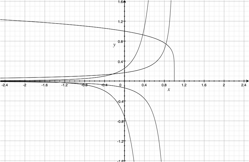
Figure 1: Finite time blowup for $m\geq 1$ along $x=t$.

and so on.

Extending $F_{4}$ on the positive real axis,

$$F_{4}(t)=\begin{cases}\pm\sqrt[6]{6\,{\it C_{1}}\,\sqrt{c_{{4}}}-6\,t\sqrt{c_{{4}}}}\quad&\text{if}\,t\in[0,C_{1}]\\ 0\quad&\text{if}\,t\in(C_{1},\infty)\\ \end{cases}$$

The above solutions with the extension $F_{4}(t)=0$ on $(C_{1},\infty)$ for $C_{1}>0$ serves as a counterexample to the smoothness assumption in one of the Millennium problems of the Clay Institute for the Navier Stokes equations. Here $u_{z}$ is not in $C^{m}$ for $m\in\{1,2,3,\dots\}$ as higher derivatives of $F_{4}(t)$ blow up in finite time for two of the four real solutions. The above Figure shows these functions and their growth.

4 Time dependent $\omega_{3}$ vorticity

If the vorticity is time dependent by choosing $u_{x}$ and $u_{y}$ as,

$$\begin{matrix}u_{x}=\sin\left[\left(n^{2}-\left(\frac{z}{\pi}\right)^{2}\right)x\right]\sin\left[\left(n^{2}-\left(\frac{x}{\pi}\right)^{2}\right)y\right]\times\\ \sin\left[\left(n^{2}-\left(\frac{y}{\pi}\right)^{2}\right)z\right]\frac{F_{x}(x,y,z)}{\left(n^{2}-\left(\frac{y}{\pi}\right)^{2}\right)z}+\eta\ y\ (1-t)^{1/6}\end{matrix}$$ (26)

$$\begin{matrix}u_{y}=\sin\left[\left(n^{2}-\left(\frac{z}{\pi}\right)^{2}\right)x\right]\sin\left[\left(n^{2}-\left(\frac{x}{\pi}\right)^{2}\right)y\right]\times\\ \sin\left[\left(n^{2}-\left(\frac{y}{\pi}\right)^{2}\right)z\right]\frac{F_{y}(x,y,z)}{\left(n^{2}-\left(\frac{y}{\pi}\right)^{2}\right)z}+\eta\ x\ (1-t)^{1/6}\end{matrix}$$ (27)

where $x=n\pi$, $y=n\pi$ and $z=n\pi$ on the wall of each cell or box of Lattice for $n\in\mathbb{R}$. Here the arbitrariness of $n$ implies that the volume $\Omega$ is any bounded and general (cube) subset of $\mathbb{R}^{3}$. This proves that $\Gamma_{1}=-\Gamma_{2}$. The tensor product volume integral in $\Gamma_{3}$ need not be zero by choice of $F_{x}(x,y,z)$ and $F_{y}(x,y,z)$, however in $\Gamma_{3}$, the second surface integral has a factor of $u^{2}_{z}$ due to three components of $\vec{b}$ for which the first two are zero. The first surface integral in $\Gamma_{3}$ is converted to a volume integral and Poisson’s equation in $x,y$ is used. Specifically for $u_{x}$ and $u_{y}$ selected, the third partial derivative of these functions wrt to $z$ is non zero. Substitution of $u_{x}$ and $u_{y}$ into Eq.(15) modulo $\Gamma_{3}$, division by $\eta$ and letting $\eta$ tend to infinity produces a general separable solution for $u_{z}$ in the form $u_{z}=g(x)h(y)k(z)f(t)$. Note that for $u_{x}$, $u_{y}$ in Eqs (16)-(17) after substitution in Eq (15) that two integrals must be solved for algebraically in sequence with subsequent differentiation wrt $z$, so that an entire non-integral pde results. Now, $u_{x}$, $u_{y}$ are zero on cell walls of the Lattice and at $t=1$. Note that the $\frac{sin(\alpha)}{\alpha}$ forms are extended for each sine factor so that the velocities are zero on all faces of the cells in the lattice.
Substituting the general form of $u_{z}$, and the specific forms for $u_{x}$ and $u_{y}$ into $\Gamma_{3}$ which involves integration over the volume of the union of all cells or boxes, we can obtain an ODE in $u_{z}$, which is,

$$C^{2}A_{2}\frac{df(t)}{dt}f(t)=C^{2}f(t)^{2}\left(A_{1}+f(t)\ (-2A)\right)$$ (28)

with constants due to integration over the volume in $\Gamma_{3}$: $C$, $A_{1}$, $A$ and $A_{2}$. $A\in\mathbb{R}$. It is noteworthy to mention that for tensor product term in $\Gamma_{3}$ the $\frac{u^{2}_{z}}{\eta^{3}}$ term vanishes in the $\eta$ limit. Also $u_{x}$ and $u_{y}$ are evaluated at $t=1$ giving a $1/\eta^{2}$ term on both sides of Eq.(28). Here the general solution is,

$$f(t)=\frac{A_{1}}{\text{e}^{-\frac{A_{1}t}{A_{2}}}C_{1}\ A_{1}+2A}$$ (29)

where $C_{1}$ is positive. Applying initial condition for arbitrarily large data, given $\epsilon>0$, $A_{1}=-\frac{2A}{C_{1}}-\epsilon$.
Of course the smaller the $\epsilon$ value the larger the data value. Substituting gives blowup times as,

$$t=-\frac{\ln\left(-\frac{2A}{\left(-\frac{2A}{C_{1}}-\epsilon\right)C_{1}}\right)A_{2}}{-\frac{2A}{C_{1}}-\epsilon}$$ (30)

The term $C_{1}>0$ when expanding $\ln$ in terms of positive $A$(no complex functions are considered). The term $A_{2}$ depends on general inputs $u_{x}$, $u_{y}$, wheras $A_{1}$ depends on pressure and $u_{z}$. So the $x-y$ inputs are independent of $A_{1}$ and possible positive blowup times exist. Finally, it is known that for a finite time singularity solution to the Navier-Stokes equations that the normalized pressure becomes unbounded from below, see [11].

5 Appendix 1-Maple Code for Wave Equation Equivalence of 3D Navier-Stokes Equations

⬇

#program to Solve Equation Eq.$(\ref{11})$;

#Second partial derivative of Pressure wrt to z:

# Use Poisson Equation

solve(simplify(%), $\delta^{2}$)

subs($\delta$=1,%)

simplify(%)-1

simplify(%)

numer(%)

simplify(%)

#Factor out $u^{2}_{z}$ and use Hardy Inequality

solve(%,$uz(x,y,z,t)^{2}$)

$subs(\left({\frac{\partial}{\partial z}}{\it ux}\left(x,y,z,t\right)\right){\it ux}\left(x,y,z,t\right)+{\it uy}\left(x,y,z,t\right){\frac{\partial}{\partial z}}{\it uy}\left(x,y,z,t\right)$ =Y,%)

solve(%,Y)

simplify(%)

$-2\,\left({\frac{\partial^{2}}{\partial{t}^{2}}}{\it uz}\left(x,y,z,t\right)\right){\frac{\partial^{3}}{\partial z\partial{t}^{2}}}{\it uz}\left(x,y,z,t\right)$+%

L2s:=simplify(%)

$subs(\left({\frac{\partial}{\partial x}}{\it uz}\left(x,y,z,t\right)\right)^{2}+\left({\frac{\partial}{\partial y}}{\it uz}\left(x,y,z,t\right)\right)^{2}+\left({\frac{\partial}{\partial z}}{\it uz}\left(x,y,z,t\right)\right)^{2}$=U,%)

solve(%,U)

L2s:=%;

#Solve resulting PDE using pdsolve command

#Introduce fourth order auxillary PDE L3 and L3W

$L_{3}\mathrel{\mathop{\mathchar 58\relax}}=c\frac{\partial^{4}u_{z}}{\partial t^{4}}-\frac{\partial^{2}u_{y}}{\partial x^{2}}-\frac{\partial^{2}u_{y}}{\partial y^{2}}-\frac{\partial^{2}u_{y}}{\partial z^{2}}=0$

$L3_{W}\mathrel{\mathop{\mathchar 58\relax}}=\frac{\partial^{2}u_{y}}{\partial t^{2}}-c\frac{\partial^{4}u_{z}}{\partial t^{4}}=0$

pdsolve(${L2s,L_{3}}$);

pdsolve(${L2s,L3_{W}}$);

#L3 and L3_W are equivalent proving,

# that we have a wave equation in $y$

# The same code above can be used by

replacing $y$ and $u_{y}$ by $x$ and $u_{x}$

respectively;

#hence we also have wave equations in $x$

and $z$.

References

- [1] T.E. Moschandreou. On the 4th Clay Millennium Problem for the Periodic Navier Stokes Equations Millennium Prize Problems. Recent Advances in Mathematical Research and Computer Science November 2021, Vol. 4, 12, 79-92 https://doi.org/10.9734/bpi/ramrcs/v4/14379D
- [2] S. Bhaumik and T. K. Sengupta, Precursor of transition to turbulence: Spatiotemporal wave front. Phys. Rev. E Published 28 April 2014 2014, 89, 043018 , 1-13, DOI: 10.1103/PhysRevE.00.003000
- [3] T.E.Moschandreou, No Finite Time Blowup for 3D Incompressible Navier Stokes Equations via Scaling Invariance. Mathematics and Statistics 2021, 9(3), 386-393.
- [4] T.E.Moschandreou and K.C. Afas, Existence of Incompressible Vortex-Class Phenomena and Variational Formulation of Raleigh–Plesset Cavitation Dynamics,Applied Mechanics. 2021, 2(3):613-629. https://doi.org/10.3390/applmech2030035
- [5] Barman HK, Aktar MS, Uddin MH, Akbar MA, Baleanu D, Osman MS. Physically significant wave solutions to the Riemann wave equations and the Landau-Ginsburg-Higgs equation.Results in Physics. 2021 Aug 1;27:104517.
- [6] Aubery D., Searching for Waves in the Incompressible Navier-Stokes Equations - The Adventure. Momentum Waves, Vol. 1, No. 1, 2019 1-29(06.12.19).
- [7] Truesdell C. and Toupin R.A., The Classical Field Theories. Encyclopedia of Physics, Vol. III/1, Springer-Verlag, 1960 226-858.
- [8] Truesdell C. and Ragagopal K.R., An introduction to the Mechanics of Fluids. Birkhauser Boston 2000.
- [9] Truesdell and Noll., The Non-Linear Field Theories of Mechanics.3 ed. Springer-Verlag 2004, 1992, 1965.
- [10] E.Miller, Finite-time blowup for smooth solutions of the Navier–Stokes equations on the whole space with linear growth at infinity Arxiv.org arXiv:2103.12237 [math.AP] 2021, 1-50.
- [11] Seregin G. and Šverák V., Navier-Stokes Equations with Lower Bounds on the Pressure. Arch. Rational Mech. Anal. 163, 2002 65-86, DOI: 10.1007/s002050200199.