Non-stationary Online Regression

Abstract

Online forecasting under changing environment has been a problem of increasing importance in many real-world applications. In this paper, we consider the meta-algorithm presented in Zhang et al. [22] combined with different subroutines. We show that an expected cumulative error of order $\tilde{\mathcal{O}}(n^{1/3}C_{n}^{2/3})$ can be obtained for non-stationary online linear regression where the total variation of parameter sequence is bounded by $C_{n}$. Our paper extends the result of online forecasting of one dimensional time-series as proposed in [2] to general $d$-dimensional non-stationary linear regression. We improve the rate $O(\sqrt{nC_{n}})$ obtained by Zhang et al. [22] and Besbes et al. [3]. We further extend our analysis to non-stationary online kernel regression. Similar to the non-stationary online regression case, we use the meta-procedure of Zhang et al. [22] combined with Kernel-AWV [16] to achieve an expected cumulative controlled by the effective dimension of the RKHS and the total variation of the sequence. To the best of our knowledge, this work is the first extension of non-stationary online regression to non-stationary kernel regression. Lastly, we evaluate our method empirically with several existing benchmarks and also compare it with the theoretical bound obtained in this paper.

1 Introduction

We consider online linear regression in a non-stationary environment. More formally, at each round $t=1,\dots,n$, the learner receives an input $x_{t}\in{\mathbb{R}}^{d}$, makes a prediction $\widehat{y}_{t}\in{\mathbb{R}}$ and receives a noisy output $y_{t}=x_{t}^{\top}\theta_{t}+Z_{t}$ where $\theta_{t}\in{\mathbb{R}}^{d}$ is some unknown parameter and $Z_{t}$ are i.i.d. sub-Gaussian noise. We are interested in minimizing the expected cumulative error

$$R_{n}(\widehat{y}_{1:n},\theta_{1:n}):=\sum_{t=1}^{n}{\mathbb{E}}\big{[}(\widehat{y}_{t}-x_{t}^{\top}\theta_{t})^{2}\big{]}\,.$$ (1)

Of course, without further assumption, the cumulative error is doomed to grow linearly in $n$. Therefore, we assume there is regularity in the signal $\theta_{1:n}=\big{(}\theta_{1},\dots,\theta_{n}\big{)}\in{\mathbb{R}}^{d\times n}$, measured by its total variation

$$TV(\theta_{1:n})=\sum_{t=2}^{n}\big{\|}\theta_{t}-\theta_{t-1}\big{\|}_{1}\,.$$ (2)

We also assume that there exists $B>0$ such that for all $t\geq 1$, $\|\theta_{t}\|_{1}\leq B$. We emphasize that apart from boundedness in $\ell_{1}$-norm and in total variation, we do not make any assumption on the sequence $\theta_{1:n}$. The latter is arbitrary and may be chosen by an adversary.

Related Works

Online prediction of arbitrary time-series has already been well studied by the online learning and optimization communities and we refer to the monographs [6, 10] and references therein for detailed overviews. A very large part of the existing work only deals with stationary environment, in which the learner’s performance is compared with respect to some fixed strategy that does not evolve over time. Thanks to many applications (e.g. web marketing or electricity forecasting), designing strategies that adapt to a changing environment has recently drawn considerable attention.

Online learning in a non-stationary environment was referred under different names or settings as “shifting regret”, “adaptive regret”, “dynamic regret”, or “tracking the best predictor” but most of these notions are strongly related. Some relevant works are [3, 14, 23, 7, 12, 4, 15, 18, 21]. [14] first considered shifting bounds for linear regression using projected mirror descent. [23] provides dynamic regret guarantees for any convex losses for projected online gradient descent. Most of these work considered however non noisy observations (or gradients), as we consider. [3] proved matching upper and lower bounds for the dynamic regret with noisy observations. They provide dynamic regret bounds of order $TV(\theta_{1:n})^{1/3}n^{2/3}$ for convex losses and $\sqrt{TV(\theta_{1:n})n}$ for strongly convex losses. The latter was generalized to exp-concave losses by [22].

Contributions

Most of the above works consider the regret, while here we consider the cumulative error (1). In other words, in our case, the performance of the player is only compared with respect to the true underlying sequence $\theta_{1:n}$ which must have low total variation. This assumption allows us to prove stronger guarantees. Indeed, in the one-dimensional setting of online forecasting of a time-series with square loss, [2] could prove that the optimal rate of order $TV(\theta_{1:n})^{2/3}n^{1/3}$ instead of $\sqrt{TV(\theta_{1:n})n}$ for the cumulative error (1). Their technique is based on change point detection via wavelets and heavily relies on their simple setting (one dimension, no input $x_{t}$).

In this work, we generalize the result of [2] to online linear regression in dimension $d$ and to reproducing kernel Hilbert spaces (RKHS). We ended up by using the meta-procedures of [11] and [22] for exp-concave loss functions, combined with well-chosen subroutines. Carrying a careful regret analysis in our setting, we achieve the optimal error of [2].

Finally, in Section 4, we corroborate our theoretical results on numerical simulations.

2 Warm-up: Online Prediction of Non-Stationary Time Series

In this section, we discuss the relevant background to our work and simple intuition for $1$-dimensional problem. However, before going into the details of our approach, we first discuss the work of Baby and Wang [2] which considers one dimensional non-stationary online linear regression.

2.1 ARROWS [2]

ARROWS considers to solve the problem of online forecasting of sequences of length $n$ whose total-variation (TV) is at most $n$. The observed output is the noise contaminated version of original input sequence $\theta_{i}$ for $i$ in $[n]$. ARROWS considers to predict via the moving average of the output in an interval. If the total-variation within that time interval is small then the moving average in that time interval is reasonably good prediction to minimize the cumulative squared error. For that reason, the algorithm needs to detect intervals which has low total variation. This task of detection is accomplished by constructing a lower bound of TV which acts like a threshold to restart the averaging and hence acts like a non-linearity which can capture the non-linear variation in the sequence. The estimation of the lower bound is based on computing of Haar coefficients as it smooths the adjacent regions of a signal and then taking difference between them. A slightly modified version of the soft threshold estimator from from Donoho et al. [8] is considered for oracle estimator.

Overall, the restart strategy based on change point detection using Haar coefficients proposed in this work achieves the optimal error however, the approach is very hard to extend beyond one dimensional regression problem. Another drawback this work has is that ARROWS requires to know the noise level sigma to tun the algorithm even in one dimensional forecasting problem. To know the exact noise level is an unrealistic assumption in real life problems. We address here these two concerns.

2.2 One-Dimensional Intuition

In this section, we consider the simpler case with $d=1$ and $x_{t}=1$ that was already considered by [2] as a warm up to understand the intuition behind our algorithm. Let us now define the formal problem. The problem formulation looks as: $y_{t}=\theta_{t}+Z_{t}$ for $t=1,\cdots,n$ and $Z_{t}$ be independent $\sigma$ sub-Gaussian random variables. The goal of the problem is to recover $\theta_{t}$ by minimizing the cumulative error $R_{n}(\widehat{y}_{1:n},\theta_{1:n})=\sum_{t=1}^{T}{\mathbb{E}}\big{[}(\widehat{y}_{t}-\theta_{t})^{2}\big{]}$.

Lower-bound and previous results

In [19], the authors first prove that using online gradient descent with fixed restart (as considered by [3]) is sub-optimal in this setting. Their theorem 2 shows a cumulative error for OGD with fixed restart of order $\tilde{\mathcal{O}}(B^{2}+TV(\theta_{1:n})^{2}+\sigma TV(\theta_{1:n})\sqrt{n})$, where $B$ is an upper-bound on $\|\theta_{1}\|_{1}$. Yet, they also prove the following lower-bound.

Proposition 1 ([2, Proposition 2])

Let $n\geq 2$, $\sigma>0$, and $B,C_{n}>0$ such that $\min\{B,C_{n}\}>2\pi\sigma$. Then, there is a universal constant $c$ such that, for any forecaster, there exists a sequence $\theta_{1},\dots,\theta_{n}$ such that $TV(\theta_{1:n})\leq C_{n}$ and

$$R_{n}\big{(}\widehat{y}_{1:n},\theta_{1:n}\big{)}\geq c(B^{2}+C_{n}^{2}+\sigma^{2}\log n+n^{1/3}C_{n}^{2/3}\sigma^{4/3}).$$

Our aim is to address the two major challenges of ARROWS discussed previously (address general $d$-dimensional problems and no need to know the exact noise level $\sigma$) while achieving an optimal error of order $O(n^{1/3}C_{n}^{2/3})$.

An hypothetical forecaster which achieves optimal error

Let $m\geq 1$. We first analyse the approximation error obtained by an hypothetical forecaster that produces moving average with at most $m$ restarts. It first computes a sequence of restart times $1=t_{1}\leq t_{2}\leq\dots\leq t_{m+1}=n+1$ such that

$$TV\big{(}\theta_{t_{i}:(t_{i+1}-1)}\big{)}\leq\frac{TV(\theta_{1:n})}{m}\,,$$ (3)

for all $1\leq i\leq m$ and then forms the prediction $\tilde{y}_{t}$ for $t\in\{t_{i}+1,\dots,t_{i+1}\}$

$$\tilde{y}_{t}:=\bar{y}_{t_{i}:(t-1)}~{}\text{where}~{}\bar{y}_{t_{i}:(t-1)}:=\frac{1}{t-t_{i}}\sum_{k=t_{i}}^{t-1}y_{k}\,.$$ (4)

We would assume the existence of similar hypothetical forecaster for non-stationary online linear regression (section 3.1) and non-stationary online kernel regression (section 3.2) with slight variation in the prediction function. Of course this forecaster is not practical since the restart times $t_{i}$ are unknown.

In Theorem 5 stated in Appendix A, we show that for $m\approx n^{1/3}C_{n}^{2/3}$, this hypothetical forecaster achieves the same optimal error of Proposition 1,

$$R_{n}(\tilde{y}_{1:n},\theta_{1:n})\leq O(n^{1/3}C_{n}^{2/3})\,,$$ (5)

as was already obtained by [2]. Of course, it remains to estimate the restart times $t_{i}$.

A meta-aggregation algorithm to learn the restart times

Contrary to [2], which uses a change point detection method, we propose to do so by using meta-aggregation algorithms from non-stationary online learning such Follow the Leading History (FLH) [11] based on exponential weights and presented in Algorithm 1.

Input: black box algorithm $\mathcal{A}$, learning parameter $\eta>0$

1

2Init: $S_{0}=\emptyset$

3for  $t=1,\dots,n$ do

4       Start a new instance of algorithm $\mathcal{A}$ denoted $\mathcal{A}_{t}$ and assign weight $\widehat{p}_{t}(t)=\frac{1}{t}$.

5      Normalize the weight of each expert $j\in[t-1]:=\{1,\dots,t-1\}$

$$\textstyle{\widehat{p}_{t}(j):=\big{(}1-\frac{1}{t}\big{)}\frac{p_{t}(j)}{\sum_{j\in[t-1]}p_{t}(j)}}$$

6      Observe $x_{t}$ and get the prediction $\tilde{y}_{t}(i)$ from each black box algorithm $\mathcal{A}_{i},i\in[t-1]$.

7      Predict $\widehat{y}_{t}=\sum_{i\in[t-1]}\widehat{p}_{t}(i)\tilde{y}_{t}(i)$ and observe $y_{t}\in{\mathbb{R}}$.

8      Update the weights for each $i\in[t-1]$

$$p_{t+1}(i)=p_{t}(i)\exp\big{(}-\eta(y_{t}-\tilde{y}_{t}(i))^{2}\big{)}\,.$$

Algorithm 1 Follow the Leading History (FLH) [11]

Basically, FLH is a meta-aggregation procedure that considers a subroutine algorithm, called $\mathcal{A}$, producing a prediction based on past observations. $\mathcal{A}$ can be any online learning algorithm that aims at minimizing the static regret, that is the excess cumulative error compared to a fixed parameter. The role of the meta-algorithm is to learn the restarts. To do so, at each round $t\geq 1$, FLH builds a new expert (step 3 of Alg. 2) that applies $\mathcal{A}$ on the sequence of observations $y_{t},\dots,y_{n}$ (that is by not considering the past data before round $t$). This new expert is assigned a weight $1/t$ and the weights of previous experts are normalized so that they sum to 1 (step 4). All the experts are then combined using a standard exponentially weighted average algorithm (step 6 of Alg. 2). The prediction of FLH is finally obtained (step 8) by forming a convex combination of the expert predictions. The number of active experts grow linearly with time. In Alg. 2, we also present IFLH, introduced by [22], which improves the computational complexity by removing experts over time.

In Theorem 1, we show that a cumulative error of optimal order $\tilde{O}(C_{n}^{2/3}n^{1/3})$ can be achieved by applying FLH with moving averaged (4) as subroutines.

Theorem 1

Let $\theta_{1:n}\in{\mathbb{R}}^{n}$ such that $TV(\theta_{1:n})\leq C_{n}$. Assume that $|\theta_{t}|\leq B$ for all $t\geq 1$. If moving average predictions (4) are used as subroutine of Algorithm 2, the cumulative error is upper-bounded as

$$R_{n}(\widehat{y}_{1:n},\theta_{1:n})\leq O(n^{1/3}C_{n}^{2/3}\log^{2}n)\,,$$

with high probability.

Proof  First, with probability $1-\delta$, all $|y_{t}|=|\theta_{t}+Z_{t}|$ for $1\leq t\leq n$ are bounded by $C\sqrt{\log n}$ for some constant $C$ depending on $B$ and $\sigma^{2}$. Thus, $y\mapsto(y-y_{t})^{2}$ are $\alpha$-exp-concave with $\alpha=C^{\prime}/(\log(n/\delta))$ for some $C^{\prime}>0$. Let $m\approx n^{1/3}C_{n}^{2/3}$ and $t_{1},\dots,t_{m}$ be as defined in (3) and (5) (see also Thm. 5). From Claim 3.1 of [11], we have for any $i=1,\dots,m$

$$\sum_{t=t_{i}}^{t_{i+1}-1}(\widehat{y}_{t}-y_{t})^{2}-(\tilde{y}_{t}(t_{i})-y_{t})^{2}\leq\frac{3\log n}{\alpha}\leq O(\log^{2}n)\,.$$

Therefore, summing over $i=1,\dots,m$ and using that the subroutines are moving averages (i.e., $\tilde{y}_{t}(t_{i})=\bar{y}_{t_{i}:(t-1)}$) and the definition of $\tilde{y}_{t}$ in (4), we get

$$\sum_{t=1}^{n}(\widehat{y}_{t}-y_{t})^{2}-(\tilde{y}_{t}-y_{t})^{2}\leq O(m\log^{2}n)\,.$$ (6)

Thus, because $Z_{t}=y_{t}-\theta_{t}$ is independent of $\widehat{y}_{t}$

$$R_{n}(\widehat{y}_{1:n},\theta_{1:n}):=\sum_{t=1}^{n}{\mathbb{E}}\big{[}(\widehat{y}_{t}-y_{t}+y_{t}-\theta_{t})^{2}\big{]}$$

$$=\sum_{t=1}^{n}{\mathbb{E}}\big{[}(\widehat{y}_{t}-y_{t})^{2}-(y_{t}-\theta_{t})^{2}\big{]}$$

$$=\sum_{t=1}^{n}{\mathbb{E}}\big{[}(\widehat{y}_{t}-y_{t})^{2}-(\tilde{y}_{t}-y_{t})^{2}$$

$$\hskip 56.9055pt+(\tilde{y}_{t}-y_{t})^{2}-(y_{t}-\theta_{t})^{2}\big{]}$$

$$\stackrel{{\scriptstyle\eqref{eq:reg_hazan}}}{{\leq}}O(m(\log n)^{2})+\sum_{t=1}^{n}{\mathbb{E}}\big{[}(\tilde{y}_{t}-y_{t})^{2}-(y_{t}-\theta_{t})^{2}\big{]}\,.$$

It only remains to show that the last term corresponds to $R_{n}(\tilde{y}_{1:n},\theta_{1:n}):=\sum_{t=1}^{n}{\mathbb{E}}\big{[}(\tilde{y}_{t}-\theta_{t})^{2}\big{]}$ and apply Inequality (5). Expending the squares, it indeed yields

$${\mathbb{E}}\big{[} (\tilde{y}_{t}-y_{t})^{2}-(y_{t}-\theta_{t})^{2}\big{]}={\mathbb{E}}\big{[}\tilde{y}_{t}^{2}+2(\theta_{t}-\tilde{y}_{t})y_{t}-\theta_{t}^{2}\big{]}$$

$$={\mathbb{E}}\big{[}\tilde{y}_{t}^{2}+2(\theta_{t}-\tilde{y}_{t})(\theta_{t}+Z_{t})-\theta_{t}^{2}\big{]}$$

$$={\mathbb{E}}\big{[}(\tilde{y}_{t}-\theta_{t})^{2}\big{]}\,,$$

where the last equality is because ${\mathbb{E}}[Z_{t}]=0$ and $Z_{t}$ is independent from $\tilde{y}_{t}$ and $\theta_{t}$.  

3 Non-Stationary Online Regression

In this section, we discuss more general problem of non-stationary online regression. We consider the following problem :

$$y_{t}=g_{t}(x_{t})+Z_{t}$$ (7)

where $g_{t}:\mathbb{R}^{d}\rightarrow\mathbb{R}$ is a non-linear function and $Z_{t}$ be independent $\sigma$-subGaussian random variables in one dimension with ${\mathbb{E}}[Z_{t}]=0$. Similar to the previous section, the goal in this section would be to track the sequence of $g_{t}$ with $\widehat{g}_{t}$ for all $t$ such that $\widehat{y}_{t}=\widehat{g}_{t}(x_{t})$ to minimize the expected cumulative error $R_{n}(\widehat{y}_{1:n},\theta_{1:n})$ with respect to the unobserved output $g_{t}$ after $n$ time steps which we define as follow:

$$R_{n}(\widehat{y}_{1:n},g_{1:n})=\sum_{t=1}^{n}\mathbb{E}\left[(\widehat{y}_{t}-{g}_{t}(x_{t}))^{2}\right]$$

$$=\sum_{t=1}^{n}\mathbb{E}\left[(\widehat{g}_{t}(x_{t})-{g}_{t}(x_{t}))^{2}\right].$$ (8)

However, we need to remember that we observe $g_{t}(x_{t})$ only after perturbed through some noise variable $Z_{t}$. Hence, we need to decompose our regret in terms of the observed response $y_{t}$. Bias-variance decomposition directly provides the decomposition in terms of the observed variable $y_{t}$. Proof is given in Appendix B.

Lemma 1

For any sequence of functions $\tilde{g}_{t}:\mathbb{R}^{d}\rightarrow\mathbb{R}$ for $t\in[n]$ independent of $Z_{t}$ for all $t$, the cumulative error (8) can be decomposed as follows:

$$R_{n}(\widehat{y}_{1:n},g_{1:n})=\sum_{t=1}^{n}\mathbb{E}\left[(\widehat{y}_{t}-{y}_{t})^{2}-(\tilde{g}_{t}(x_{t})-{y}_{t})^{2}\right]$$

$$+\sum_{t=1}^{n}\mathbb{E}\left[(\tilde{g}_{t}(x_{t})-{g}_{t}(x_{t}))^{2}\right].$$

3.1 Non-stationary Linear Regression

Input: black box algorithm $\mathcal{A}$, learning parameter $\eta>0$

1

2Init: $S_{0}=\emptyset$

3for  $t=1,\dots,n$ do

4       Start a new instance of algorithm $\mathcal{A}$ denoted $\mathcal{A}_{t}$ and assign weight $\widehat{p}_{t}(t)=\frac{1}{t}$.

5      Define its ending time as $\tau_{t}:=t+2^{k}$ where $k:=\min\{k\geq 0\ \text{s.t}\ c_{k}>0\}$ and $t:=\sum_{i=1}^{\infty}c_{k}2^{k}$ is the binary representation of $t$.

6      Define the set of active experts $S_{t}:=\{1\leq i\leq t:\ \tau_{i}>t\}$

7      Normalize the weight of each active expert $j\in S_{t}\setminus\{t\}$

$$\widehat{p}_{t}(j):=\big{(}1-\frac{1}{t}\big{)}\frac{p_{t}(j)}{\sum_{j\in S_{t}\setminus\{t\}}p_{t}(j)}$$

8      Observe $x_{t}$ and get the prediction $\tilde{y}_{t}(i)$ from each black box algorithm $\mathcal{A}_{i},i\in S_{t}$.

9      Predict $\widehat{y}_{t}=\sum_{i\in S_{t}}\widehat{p}_{t}(i)\tilde{y}_{t}(i)$ and observe $y_{t}\in{\mathbb{R}}$.

10      Update the weights for each $i\in S_{t}$

$$p_{t+1}(i)=p_{t}(i)\exp\big{(}-\eta(y_{t}-\tilde{y}_{t}(i))^{2}\big{)}\,.$$

Algorithm 2 IFLH – Improved Following the Leading History (binary base) [22]

In Lemma 1, we provided the general bias-variance decomposition result for squared loss while computing expected cumulative error. In this section, we will specifically discuss the result for linear predictor $\theta_{t}$ for all $t$ i.e. we assume that $g_{t}$ is linear function for all $t$. Hence, the problem can be formulated as follows. At each step $t\geq 1$, the learner observes $x_{t}\in{\mathbb{R}}^{d}$, predicts $\widehat{y}_{t}=x_{t}^{\top}\widehat{\theta}_{t}$ and observes

$$y_{t}=x_{t}^{\top}\theta_{t}+Z_{t}\,$$ (9)

where $Z_{t}$ be independent $\sigma$-subGaussian zero mean random variable. We assume $\theta_{1},\dots,\theta_{n}\in{\mathbb{R}}^{d}$ such that $TV(\theta_{1:n})=\sum_{t=2}^{n}\|\theta_{t}-\theta_{t-1}\|_{1}\leq C_{n}$ and $\|\theta_{t}\|\leq B$ for all $t\geq 1$. The goal is to control the cumulative error with respect to the unobserved outputs $\tilde{y}_{t}=x_{t}^{\top}\theta_{t}=y_{t}-Z_{t}.$ We substitute $g_{t}(x_{t})$ with $x_{t}^{\top}\theta_{t}$ in Equation (8) and denote the prediction function $\widehat{g}_{t}(x_{t})=x_{t}^{\top}\widehat{\theta}_{t}=\widehat{y}_{t}$. Hence, the expected cumulative error $R_{n}(\widehat{y}_{1:n},g_{1:n})$ can be written as

$$\sum_{t=1}^{n}{\mathbb{E}}\Big{[}(\widehat{y}_{t}-\tilde{y}_{t})^{2}\Big{]}=\sum_{t=1}^{n}{\mathbb{E}}\Big{[}\big{(}(\widehat{\theta}_{t}-\theta_{t})^{\top}x_{t}\big{)}^{2}\Big{]}\,.$$

Hypothetical forecaster

We consider an hypothetical forecaster which similar to that of 1-dimensional case. It computes a sequence of restart times $1=t_{1}\leq t_{2}\leq\dots\leq t_{m+1}=n+1$ for all $1\leq i\leq m$ as in equation (3) and then forms the prediction $\tilde{y}_{t}$ for $t\in\{t_{i}+1,\dots,t_{i+1}\}$

$$\tilde{y}_{t}:=x_{t}^{\top}\bar{\theta}_{t}\,,$$ (10)

where $\bar{\theta}_{t}=\bar{\theta}_{t_{j}:(t_{j+1}-1)}$ for $t_{j}\leq t<t_{j+1}$ and $\bar{\theta}_{t_{j}:(t_{j+1}-1)}=\frac{1}{t_{j+1}-t_{j}}\sum_{t=t_{j}}^{t_{j+1}-1}\theta_{t}$. Below in Lemma 2, we show that the cumulative error can be controlled with respect to this hypothetical forecaster.

Lemma 2 (Adaptive Restart in $d$-dimension)

Let $X,B>0$. Assume that $\|x_{t}\|\leq X$ and $\|\theta_{t}\|\leq B$ for all $t\in[n]$. Then, there exists a sequence of restarts $1=t_{1}<\dots<t_{m}=n+1$ such that

$$\sum_{t=1}^{n}(x_{t}^{\top}\bar{\theta}_{t}-x_{t}^{\top}\theta_{t})^{2} =\sum_{j=1}^{m}\sum_{t=t_{j}}^{t_{j+1}-1}\big{(}(\bar{\theta}_{t_{j}:(t_{j+1}-1)}-\theta_{t})^{\top}x_{t}\big{)}^{2}$$

$$\leq X^{2}n\Big{(}\frac{C_{n}}{m}\Big{)}^{2}+4X^{2}B^{2}m\,,$$

where $\bar{\theta}_{t}:=\bar{\theta}_{t_{j}:(t_{j+1}-1})$ for $t_{j}\leq t\leq t_{j+1}-1$ and $\bar{\theta}_{t_{j}:(t_{j+1}-1)}=\frac{1}{t_{j+1}-t_{j}}\sum_{t=t_{j}}^{t_{j+1}-1}\theta_{t}$.

However, this forecaster cannot be computed and is only useful for the analysis since both the restart times $t_{i}$ and the parameters $\theta_{t}$ are unknown. We use meta algorithm Improved Following the Leading History (IFLH, Algorithm 2) [22] to efficiently learn the restart time which is computationally more efficient than FLH presented in Algorithm 1. To reduce the computation complexity, there is also an associated ending time for each expert in IFLH which tells that that particular expert will no longer active after its ending time. As we only have the access to the noisy gradient, we will utilize the result presented in [22, Theorem 1] with a probabilistic upper bound on the gradient to get the final upper bound on expected cumulative loss. We provide below an upper bound on the expected cumulative error.

Theorem 2

Let $n,m\geq 1$, $\sigma>0$, $B>0$, $X>0$, and $C_{n}>0$. Let $\theta_{1},\dots,\theta_{n}$ such that $TV(\theta_{1:n})\leq C_{n}$ and $\|\theta_{t}\|\leq B$. Assume that $\|x_{t}\|\leq X$ for all $t\geq 1$. Then, Alg. 2 [22] with Online Newton Step [13] as subroutine and well-tuned learning rate $\eta>0$ satisfy

$$R_{n}(\widehat{y}_{1:n},\theta_{1:n})\lesssim d^{1/3}n^{1/3}C_{n}^{2/3}(X^{2}\sigma^{2}B+X^{2}B^{2})^{1/3}\,,$$

with high probability.

Discussion:

The result presented in Theorem 2 provides an upper bound on the expected cumulative error of Alg. 2 for non-stationary online linear regression. This generalizes the result of Baby and Wang [2] which only works for one dimensional problem. Our algorithm is adaptive to the noise parameter $\sigma$ which means we do not need to know the variance $\sigma$, which is not correct for the algorithm presented in Baby and Wang [2]. While implementing the algorithm, all we need to know is the maximum value of $y_{t}$ observed so far.

On Lower Bound:

The lower bound presented in Baby and Wang [2] can be extended easily for general $d$-dimension by considering the problem of $d$-independent variables. This will simply add an extra multiplicative factor of $d$ in the lower bound (Proposition 1). Our upper-bound is thus optimal in $n,d$, and $C_{n}$. However, the dependence in $\sigma$ is worse than the one of Baby and Wang [2]. This may be due to fact that our algorithm also adapt to the noise parameter and we do not need to know $\sigma$ in our algorithm. It is an interesting question to know whether our dependence in $\sigma$ is optimal in our case and we leave it for future work.

3.2 Non-stationary Kernel Regression

In this section, we consider the case of non-stationary online kernel regression. For the input space $\mathcal{X}$ and a positive definite kernel function $\mathcal{K}:\mathcal{X}\times\mathcal{X}\rightarrow\mathbb{R}$, we denote the RKHS associated with $\mathcal{K}$ as $\mathcal{H}$. We further denote the associated feature map $\phi:\mathcal{X}\rightarrow\mathcal{H}$, such that $\mathcal{K}(x,x^{\prime})=\langle\phi(x),\phi(x^{\prime})\rangle_{\mathcal{H}}$. With slight abuse of notation, we write that $\mathcal{K}(x,x^{\prime})=\phi(x)^{\top}\phi(x^{\prime}).$ In this section, we assume that the functions $g_{t}$ lie in some RKHS $\mathcal{H}$ corresponding to the kernel $\mathcal{K}$ for all $t$. At each step $t\geq 1$, the learner observes $x_{t}\in{\mathbb{R}}^{d}$, predicts $\widehat{y}_{t}=\phi(x_{t})^{\top}\widehat{\theta}_{t}$ and observes

$$y_{t}=\phi(x_{t})^{\top}\theta_{t}+Z_{t}\,,$$ (11)

where $Z_{t}$ be independent $\sigma$-subGaussian zero mean random variable. The case we consider comes under well specified case as the optimal functions $\theta_{1},\dots,\theta_{n}\in\mathcal{H}$ lie in the same RKHS $\mathcal{H}$ corresponding to the kernel $\mathcal{K}$ where we consider our hypothesis space. We define $K_{nn}$ as $(K_{nn})_{i,j}=\langle\phi(x_{i}),\phi(x_{j})\rangle$ and $\lambda_{k}(K_{nn})$ denotes the $k$-th largest eigenvalue of $K_{nn}$. Time dependent effective dimension $d_{eff}(\lambda,s,r)$ is defined as follows,

$$d_{eff}(\lambda,s,r)=Tr(K_{s-r,s-r}(K_{s-r,s-r}+\lambda I)^{-1})\,.$$

We also assume that $TV(\theta_{1:n})=\sum_{t=2}^{n}\|\theta_{t}-\theta_{t-1}\|_{\mathcal{H}}\leq C_{n}$. The goal is to control the cumulative error with respect to the unobserved outputs $\tilde{y}_{t}=\phi(x_{t})^{\top}\theta_{t}=y_{t}-Z_{t}.$ We substitute $g_{t}(x_{t})$ with $\phi(x_{t})^{\top}\theta_{t}$ in Equation (8) and denote the prediction function with $\widehat{\theta}_{1},\cdots,\widehat{\theta}_{n}$ such that $\widehat{g}_{t}(x_{t})=\phi(x_{t})^{\top}\widehat{\theta}_{t}=\widehat{y}_{t}$. Hence, the expected cumulative error $R_{n}(\widehat{y}_{1:n},\theta_{1:n})$ can be written as

$$R_{n}(\widehat{y}_{1:n},\theta_{1:n}) =\sum_{t=1}^{n}{\mathbb{E}}\Big{[}\big{(}(\widehat{\theta}_{t}-\theta_{t})^{\top}\phi(x_{t})\big{)}^{2}\Big{]}\,.$$

For our analysis, we consider a similar hypothetical forecaster as in linear regression (see Equation (3)). The prediction $\tilde{y}_{t}$ for $t\in\{t_{i}+1,\dots,t_{i+1}\}$ is simply given as $\tilde{y}_{t}:=\phi(x_{t})^{\top}\bar{\theta}_{t}$ where $\bar{\theta}_{t}=\bar{\theta}_{t_{j}:(t_{j+1}-1)}$ for $t_{j}\leq t<t_{j+1}$. In the result given below in Lemma 3, we show that the expected cumulative error can be controlled with respect to this hypothetical forecaster given the adaptive restart.

Lemma 3 (Adaptive Restart in RKHS)

Let $B,\kappa>0$. Assume that $\|\phi(x_{t})\|^{2}\leq\kappa^{2}$, and $\|\theta_{t}\|_{\mathcal{H}}\leq B$ for all $t$. Then, there exists a sequence of restarts $1=t_{1}<\dots<t_{m}=n+1$ such that

$$\sum_{t=1}^{n}(\phi(x_{t})^{\top}\bar{\theta}_{t}-\phi(x_{t})^{\top}\theta_{t})^{2}$$

$$\qquad\qquad=\sum_{j=1}^{m}\sum_{t=t_{j}}^{t_{j+1}-1}\big{(}(\bar{\theta}_{t_{j}:(t_{j+1}-1)}-\theta_{t})^{\top}\phi(x_{t})\big{)}^{2}$$

$$\qquad\qquad\leq\kappa^{2}n\Big{(}\frac{C_{n}}{m}\Big{)}^{2}+4\kappa^{2}B^{2}m\,,$$

where $\bar{\theta}_{t}:=\bar{\theta}_{t_{j}:(t_{j+1}-1)}$ for $t_{j}\leq t<t_{j+1}$, $C_{n}\geq\sum_{t=2}^{n}\|\theta_{t}-\theta_{t-1}\|_{\mathcal{H}}$, and

$$\bar{\theta}_{t_{j}:(t_{j+1}-1)}=\frac{1}{t_{j+1}-t_{j}}\sum_{t=t_{j}}^{t_{j+1}-1}\theta_{t}.$$

As we have discussed previously, it is not possible to compute this forecaster and it will be only useful in the analysis of the algorithm. One simply has to use a meta algorithm as in [22] to learn these restart times. However, one cannot use online newton step as the black box subroutine in this meta algorithm like it was done for linear regression as the convergence of online newton step is not known for tracking prediction functions in RKHS. Hence, we use Kernel-AWV as the black box online learner [9] (see also [16]) as subroutine in Alg. 2 to estimate the prediction function. Kernel-AWV depends on a regularization parameter $\lambda>0$. Note that other subroutines designed for Online Kernel Regression such as Pros-N-Kons [5] or PKAWV [16] can be used. Below, we have the following theorem regarding the adaptive regret of least square in when the predictor function lies in RKHS.

Theorem 3

Let $\lambda>0$. For online kernel regression with square loss if for all $i\in[n]$, $y_{i}\in[-Y,Y]$ then for Algorithm 2 with Kernel-AWV [9] with regularization parameter $\lambda$ as subroutine, we have

$$\sum_{t=r}^{s}f_{t}(\theta_{t})-\sum_{t=r}^{s}f_{t}(u)\leq 8Y^{2}({p+2})\log n+\lambda p\|\theta\|^{2}$$

$$+Y^{2}pd_{eff}(\lambda,s-r)\log\left(e+\frac{en\kappa^{2}}{\lambda}\right).$$

where $[r,s]\subseteq[n]$, $p\leq\lceil\log_{2}(s-r+1)\rceil+1$ and $f_{t}(\theta)=(y_{t}-\phi(x_{t})^{\top}\theta)^{2}$.

With Theorem 5 and Lemma 3, we have the expression for upper bound on both the independent error terms which after combining together bound the overall expected cumulative error. Below, we provide our final bound on the expected cumulative error assuming the capacity condition, i.e., that the effective dimension satisfies $d_{eff}(\lambda,n)\leq({n}/{\lambda})^{\beta}$ for $\beta\in(0,1)$. The proof is given in Appendix C.

Theorem 4

Let $n,m\geq 1$, $\sigma>0$, $B>0$, $\kappa>0$, and $C_{n}>0$. Let $\theta_{1},\dots,\theta_{n}$ such that $TV(\theta_{1:n})\leq C_{n}$ and $\|\theta_{t}\|_{\mathcal{H}}\leq B$ for all $t\geq 1$. Assume also that $\|\phi(x_{t})\|_{\mathcal{H}}\leq\kappa$ for $t\geq 1$. Then , for well chosen $\eta>0$, Alg. 2 with Kernel-AWV using $\lambda=({n}/{m})^{\frac{\beta}{\beta+1}}$ satisfies

$$R_{n}(\widehat{y}_{1:n},\theta_{1:n})\leq\tilde{\mathcal{O}}\left(C_{n}^{\frac{2(\beta+1)}{2\beta+3}}n^{\frac{1}{2\beta+3}}\left(\sigma^{2}\log\frac{n}{\delta}+B^{2}\kappa^{2}\right)\right.$$

$$+\left.C_{n}^{\frac{2}{2\beta+3}}n^{\frac{2\beta+1}{2\beta+3}}B^{\frac{4(\beta+1)}{2\beta+3}}\kappa^{\frac{2}{2\beta+3}}\right)\,.$$

with probability at least $1-\delta$.

Discussion:

To the best of our knowledge, this work is the first extension of non-stationary online regression to non-stationary kernel regression. After carefully looking at the bound on the expected cumulative regret term presented in Theorem 4 and comparing it with that of non-stationary online linear regression (Theorem 2), we find that as $\beta\rightarrow 0$, we have $\lambda\rightarrow\mathcal{O}(1/d)$ and we would have the similar dependence of $C_{n}$ and $n$ in the expected cumulative error bound for linear and kernel part. However, we have a slightly worse dependent on the variance of the noise $\sigma$ in the expected cumulative error bound for non-stationary online kernel regression than that of non-stationary online linear regression part. This artefact arises due to difficulty in simultaneously choosing optimal number of restart time $m$ and regularization parameter $\lambda$. We believe that the dependence in $\sigma$ in Theorem 4 can be improved further.

As discussed in [16], the per round space and time complexities is of order $\mathcal{O}(n^{2})$ for each prediction sequence corresponding to different start times. However, the method can be made computationally more efficient by the use of Nyström approximation [16].

It is also worth pointing out that the optimal learning rate $\eta$ only depends on $B,\kappa,\delta$, and $n$ and can be optimized using standard calibration techniques (e.g., doubling trick). The regularization parameter of $\lambda$ on the other hand depends on the regularity of the Kernel. It can be calibrated by starting at each time steps $t$ in Alg. 2 several new instances of Kernel-AWV, each run with a different parameter $\lambda$ in a logarithmic grid.

(a) Soft shifts

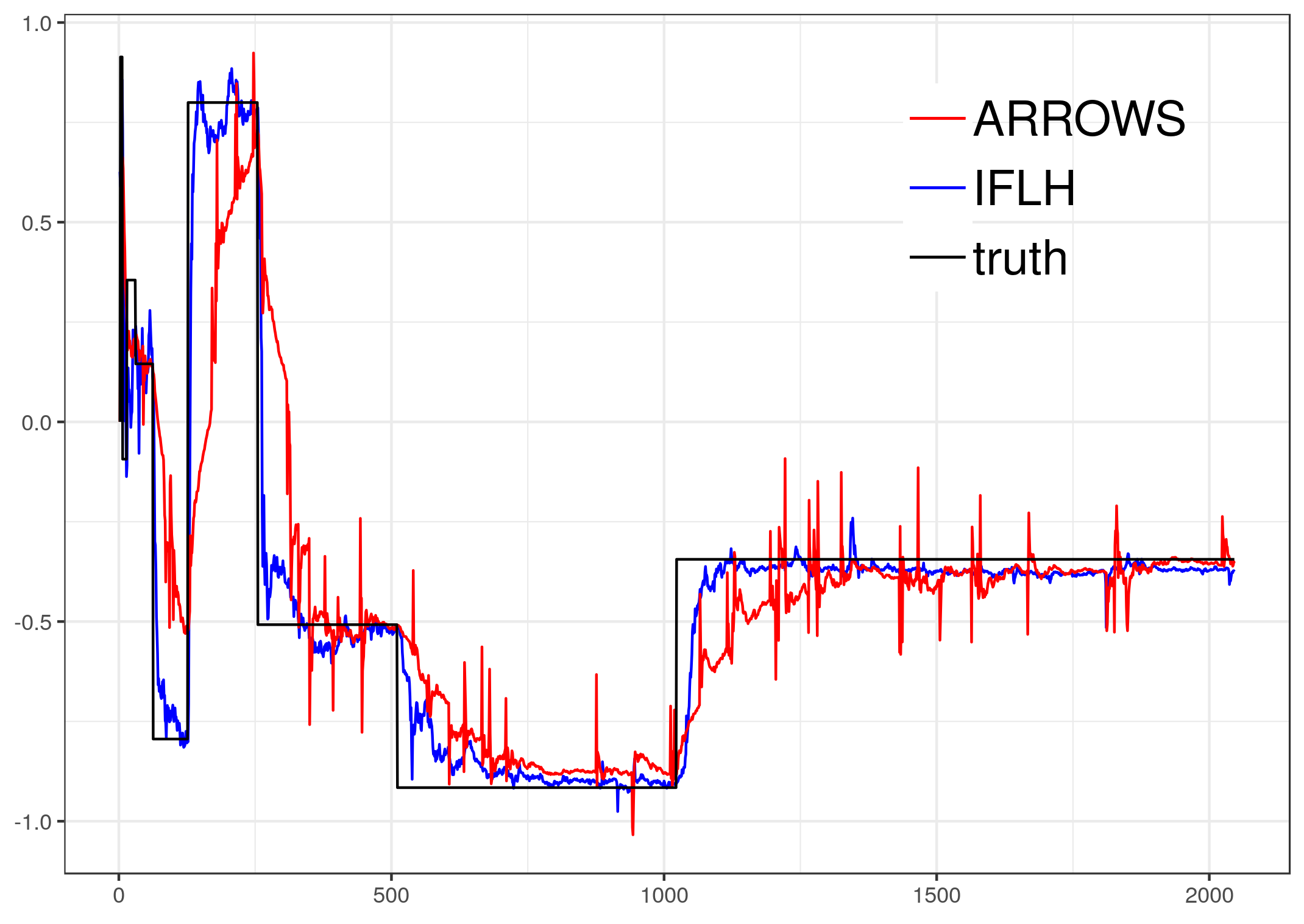
(b) Hard shifts ($m_{i}=2^{i}$, $1\!\leq\!i\!\leq\!10$)

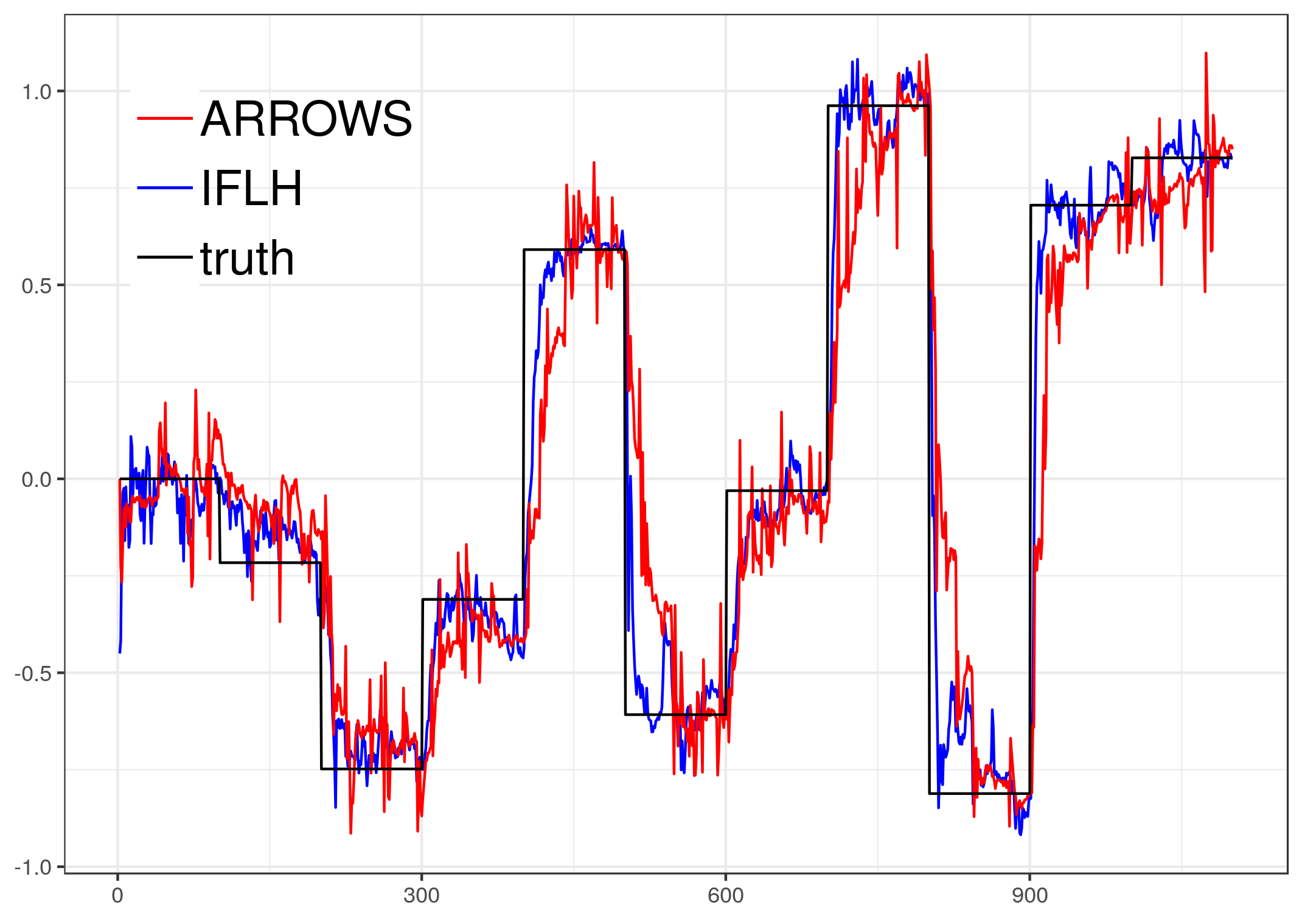
(c) Hard shifts ($m_{i}=100i$, $1\!\leq\!i\!\leq\!10$)

Figure 1: Examples of predictions obtained by the two considered algorithms (ARROWS in red and IFLH in blue) together with the one dimensional time-series to be predicted.

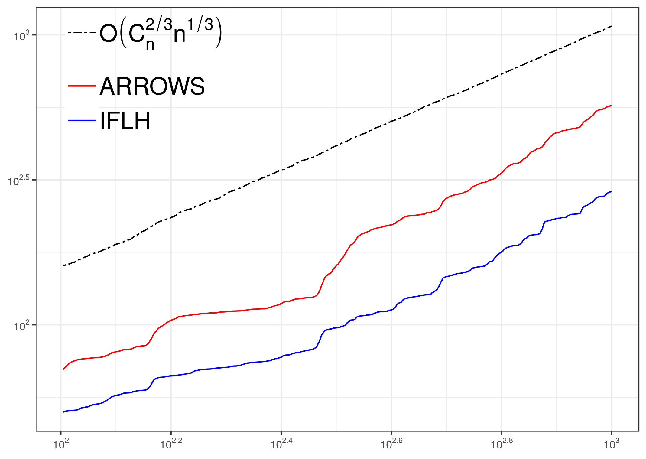
(a) Soft shifts

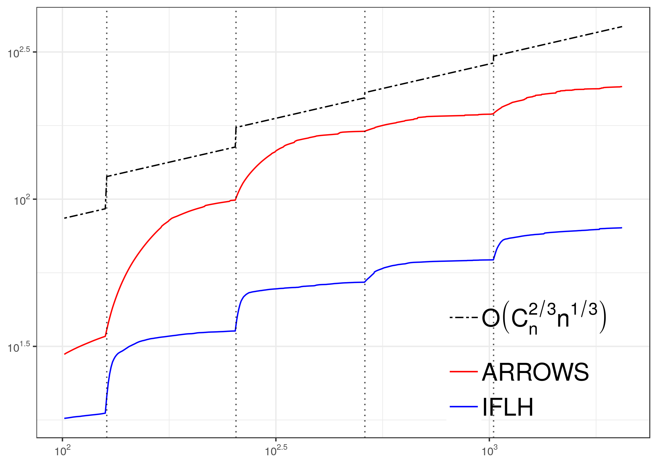
(b) Hard shifts ($m_{i}=2^{i}$, $1\!\leq\!i\!\leq\!10$)

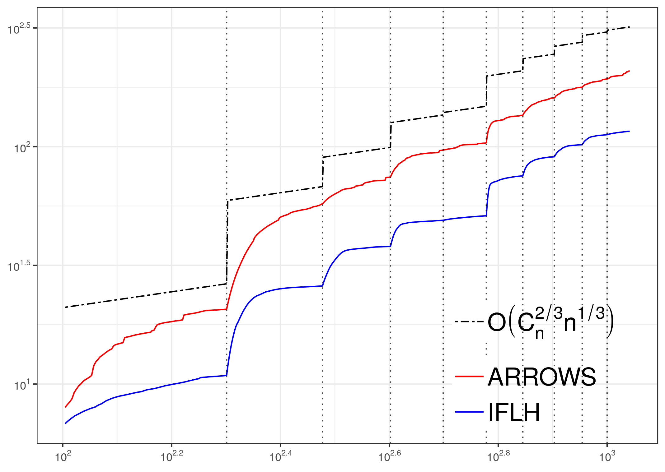
(c) Hard shifts ($m_{i}=100i$, $1\!\leq\!i\!\leq\!10$)

Figure 2: Cumulative errors suffered in average over 10 runs by the two algorithms (ARROWS in red, IFLH in blue) together with the upper bound of order $O(n^{1/3}C_{n}^{2/3})$ for one dimensional time-series.

4 Experiments

In this section, we evaluate our results on empirical simulations. We compare the theoretical bound with the performance of ARROWS [2] (wherever possible (1 dimension, no input)) and the procedure analyzed here, i.e., IFLH [22] with different subroutines (Online Newton Step [13], OGD [23], or Azoury-Warmuth-Vovk forecaster [20, 1]), and online gradient descent with fixed restart [3]. We test the algorithms on two different settings. The first one involves a non-stationary time series with continuous small changes in distribution which we call soft shifts. We use decaying innovation variance in order to observe how the algorithms react to a smooth change in the total variation. The second one involves hard and abrupt changes in distribution at well separated time intervals, we call the hard shifts.

4.1 Data Generation

Before presenting the experimental results and plots, we quickly here discuss the data generation process. Details of data generation process in the setting of soft shifting and hard shifting is given below.

Soft Shifts:

We let $\theta_{1},\dots,\theta_{n}$ be a multivariate random walk with exponential decaying variance. We set, $\theta_{t}=\theta_{t-1}+\epsilon_{t}$ with $\epsilon_{t}\sim\mathcal{N}(0,t^{-\alpha}I_{d})$ multivariate normal. The total variation of this time series is $TV=\sum_{t=2}^{n}||\theta_{t}-\theta_{t-1}||_{1}=\sum_{t=2}^{n}||\epsilon_{t}||_{1}$.

Hard Shifts:

For generating the data used in hard shifts mechanism, we split the time series $\theta_{1},...,\theta_{n}\in{\mathbb{R}}^{d}$ into $M$ chunks such that $m_{i}$ is the index of the start of the $i^{\text{th}}$ chunk. At the start of each new chunk, all coordinates $\theta_{m_{i}}(k)$ for $1\leq k\leq d$ are sampled from independent Rademacher distributions. The values of $\theta_{t}$ are then constant within a chunk. The total variation of the decision vector $\theta_{1:n}$ is $TV=\sum_{t=2}^{n}||\theta_{t}-\theta_{t-1}||_{1}=\sum_{i=2}^{M}||\theta_{m_{i}}-\theta_{m_{i-1}}||_{1}$.

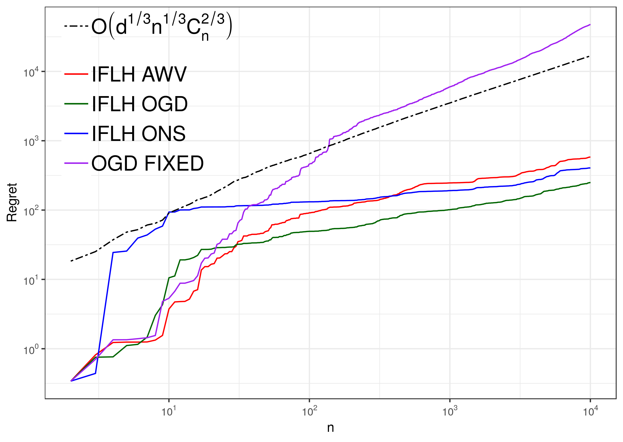
(a) $\alpha=1$ and $d=2$

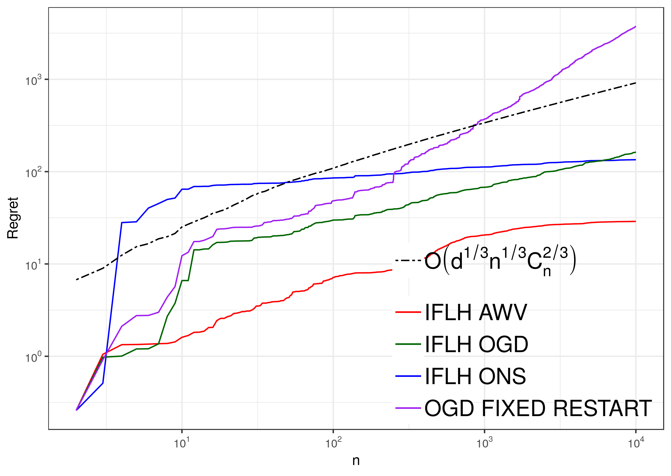
(b) $\alpha=2$ and $d=2$

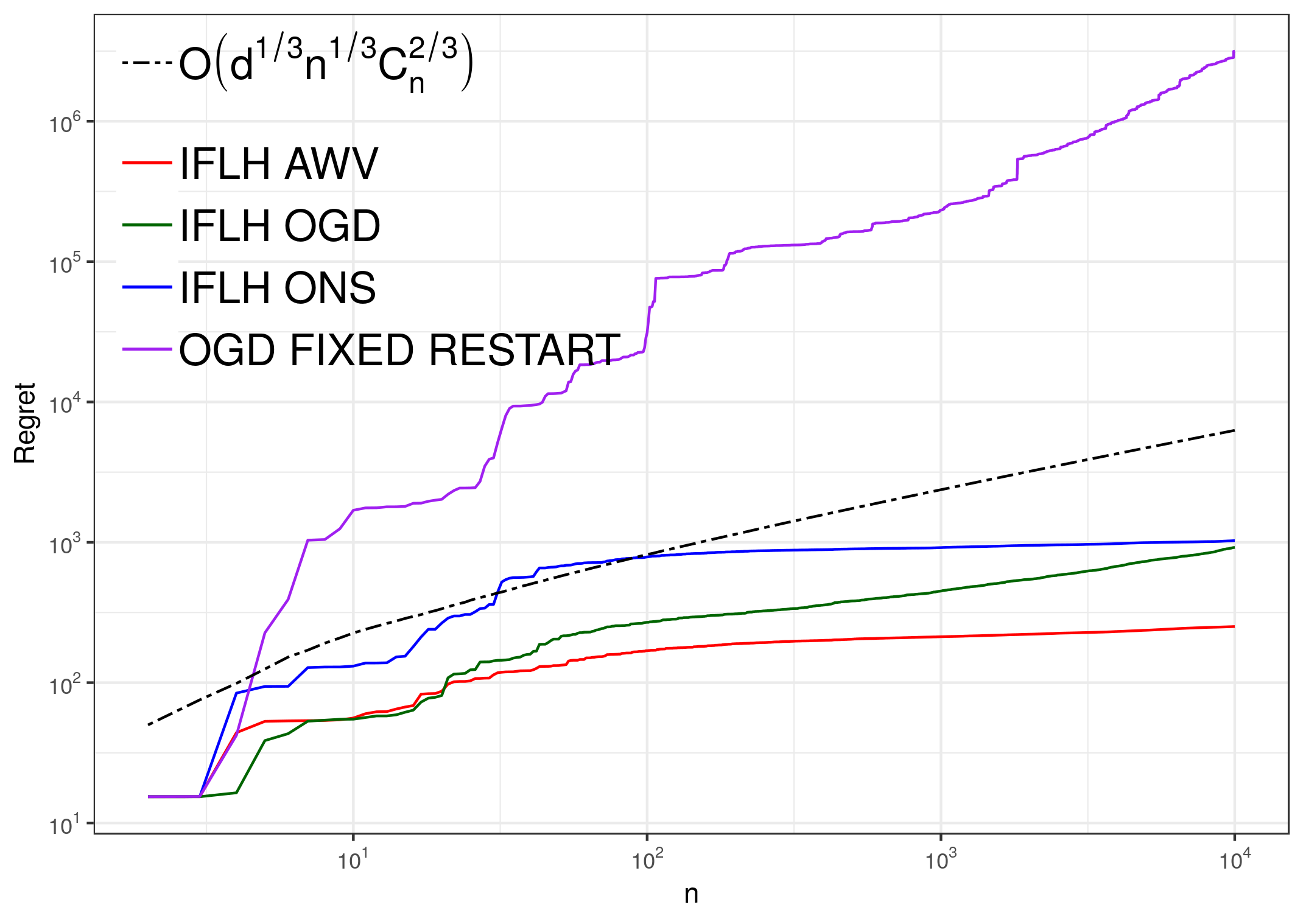
(c) $\alpha=2$ and $d=10$

Figure 3: Performances of online linear regression IFLH algorithms and OGD with fixed restart on the time series generated with the Soft Shifts for various dimension $d$ and parameter $\alpha$

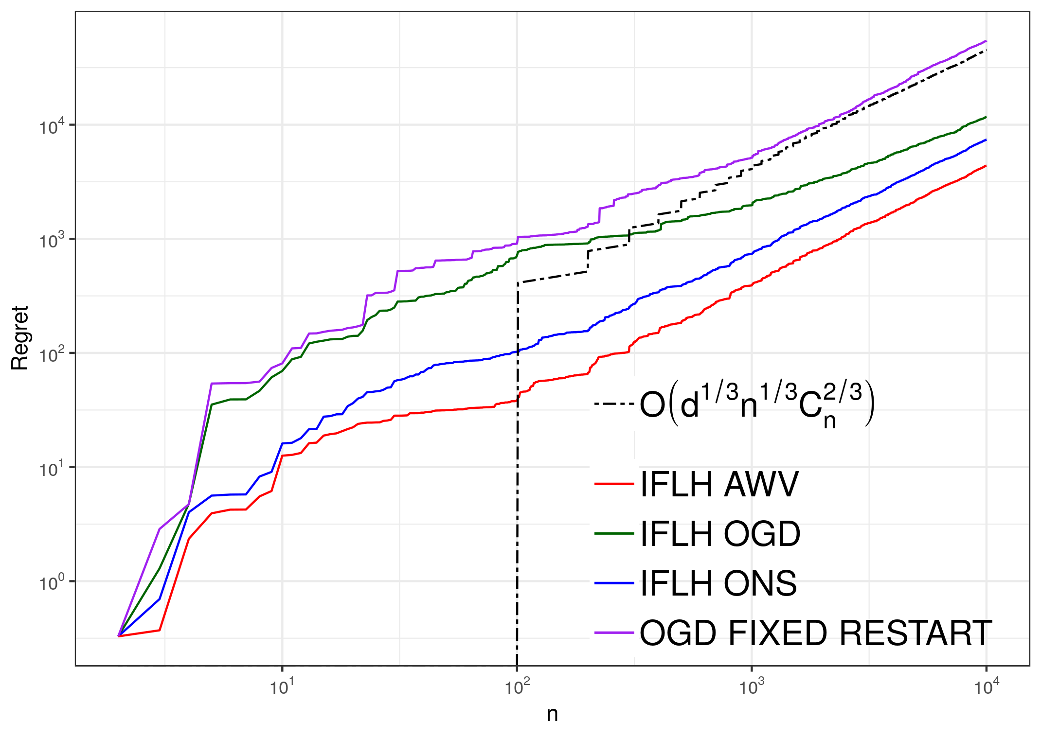
(a) $\{m_{i}=100i\,|\,1\leq i\leq 100\}$, $d=10$

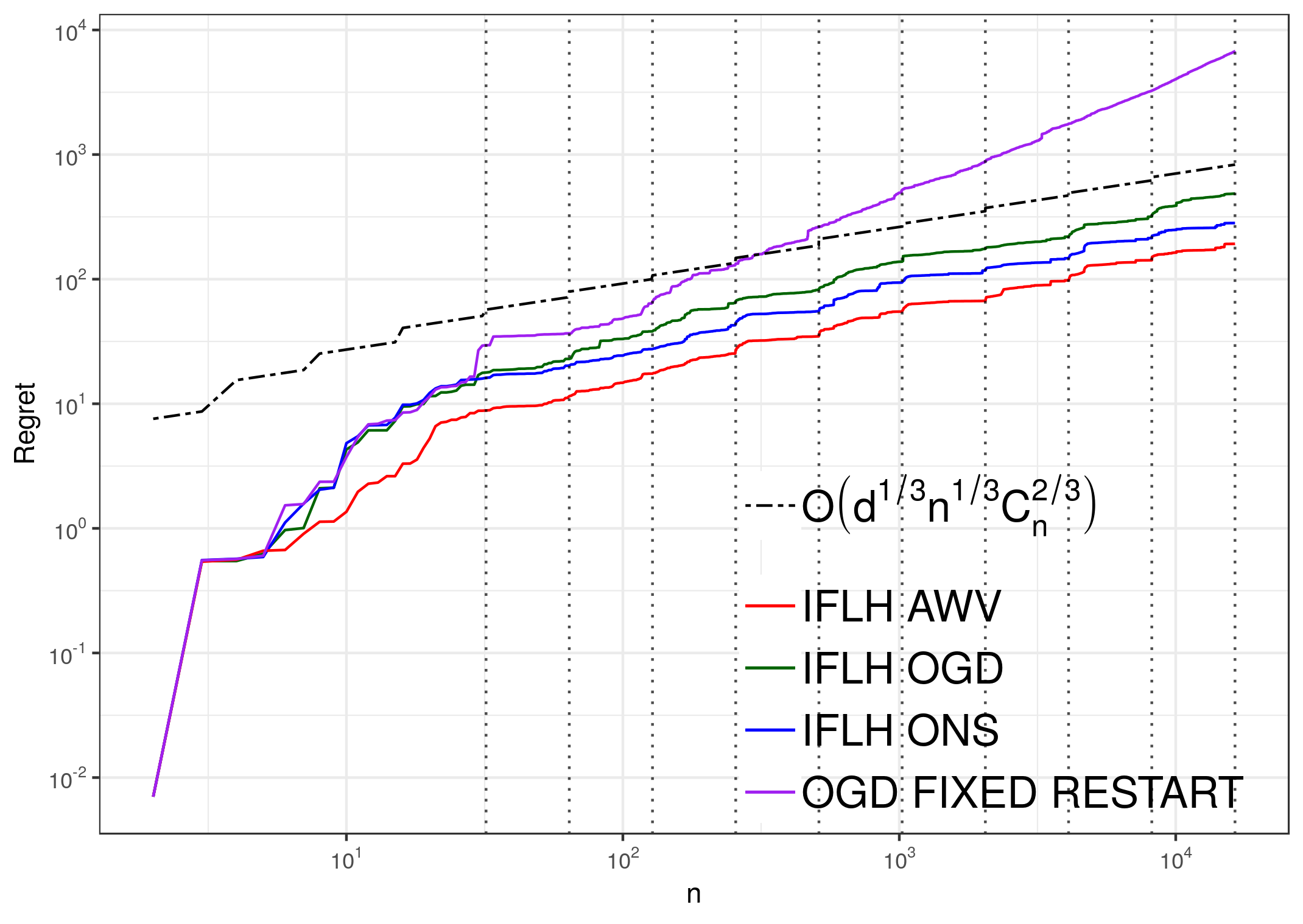
(b) $\{m_{i}=2^{i}\,|\,1\leq i\leq 14\}$, $d=2$

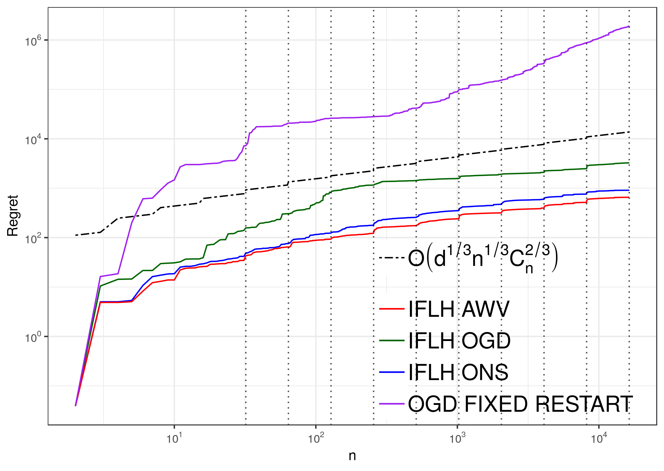
(c) $\{m_{i}=2^{i}\,|\,1\leq i\leq 14\}$, $d=10$

Figure 4: Performances of online linear regression IFLH algorithms and OGD with fixed restart on the time series generated with the Hard Shifts.

4.2 1-Dimension (Figs 1 and 2)

We use ARROWS [2] as our baseline for this part of the experiment, we compare it with our procedure proposed in Section 2, that is IFLH with moving averages as a subroutine. We recall that ARROWS was especially designed for this one dimensional setting in which it achieves the optimal rate. It also requires the variance of the noise $\sigma^{2}$ to be give beforehand which is not the case for our procedure. We average the predictions and the cumulative errors on 10 iterations over the time series. In all of our experiments, we consider the sub-Gaussian noise with standard deviation to be $\sigma=1$. We have $y_{t}=\theta_{t}+Z_{t}$ with $Z_{t}\sim\mathcal{N}(0,\sigma^{2})$. We generate data by soft shifting and hard shifts mechanism described above.

Soft Shifts:

In first part of our experiment, we generate the data by soft shifting mechanism. The parameter $\alpha$, which controls how much the time-series is non-stationary, is set to be $0.3$. This results in a slow decay of total variation of order $\sum_{t=2}^{n}t^{-\alpha}=O(n^{1-\alpha})=O(n^{0.7})$ and in an upper-bound of order $O(C_{n}^{2/3}n^{1/3})=O(n^{1-\frac{2}{3}\alpha})=O(n^{4/5})$. We can see in Figure 2(a) that IFLH reacts faster to slight changes in the time series yielding a slightly smaller cumulative error than ARROWS.

Hard Shifts:

For the second part of the experiment, we generate data using the hard shift mechanism. In Figures 1(b) and 2(b) we test IFLH and ARROWS on a time series with equal spaced shifts, whereas in Figure 1(c) and 2(c), time intervals between shifts grow exponentially with the length of the total number of shifts. It is clear from the plots that IFLH reacts faster than ARROWS to abrupt changes and manages to adapt better to stationary portions of the time series.

4.3 Online linear regression

We test IFLH [22] on the online linear regression setting with three different subroutines: Online Gradient Descent (OGD), Online Newton Steps (ONS) as well as AWV (online ridge regression). We chose these subroutines because they are well used by the online learning community for standard stationary online linear regression. Note that ONS and AWV achieve optimal regret while this is not the case for OGD which cannot take advantage of the exp-concavity of the square loss. We compare their performances with the Online Gradient Descent with fixed restart of Besbes et al. [3]. We use as batch size their theoretical result of $\left\lceil{\sigma^{-1}\sqrt{n\log n}/TV}\right\rceil$. We again consider two data generation mechanism as described above (soft shifting and hard shifting) to generate decision vectors $\theta_{t}$ for all $t$. We take the sub-Gaussian noise to be multivariate normal with $\Sigma=I_{d}$. We have

$$Y_{t}=X_{t}^{\top}\theta_{t}+Z_{t}$$

with $Z_{t}\sim\mathcal{N}(0,\Sigma)$. We take $X_{t}$ to be multivariate uniformly distributed random variables $X_{t}\sim U(-\mathbf{1},\mathbf{1})$. The expected cumulative error of OGD with fixed restart grows at a rate greater than the the theoretical upper bound of $O(d^{1/3}n^{1/3}TV^{2/3})$ proved in this paper. IFLH algorithms regrets stay below the theoretical upper bound.

Soft shifts:

In Figure 3, we vary the noise decaying parameter $\alpha$ as well as the dimension $d$ of the time series. We can clearly notice the better performance of IFLH algorithms especially with ONS and AWV as subroutine. When $\alpha=2$ for instance, the sequence of $\theta_{t}$ quickly converges and OGD with fixed restart continues on resetting which leads to the high divergence of its regret.

Hard shifts:

In experiment 4(a), we use fixed size chunks. The OGD with fixed restart algorithm performs well since the sizes of the chunks are constant and adopting a fixed restart window strategy corresponds to the setting. IFLH algorithms reacts faster to these changes and have a slightly lower regret. In 4(b) and 4(c), we use an exponentially growing size partitions. OGD with fixed restart’s regret grows at a rate bigger than the boundary line of $O(d^{1/3}n^{1/3}TV^{2/3})$. IFLH algorithms conserve a regret rate of this order.

Acknowledgments

This work was funded in part by the French government under management of Agence Nationale de la Recherche as part of the "Investissements d’avenir" program, reference ANR-19-P3IA-0001 (PRAIRIE 3IA Institute).

Appendix

Appendix A Warmup : One Dimensional Time Series

Theorem 5 (Approximation error)

Let $n,m\geq 1$, $\sigma>0$, and $C_{n}>0$. Assume that $1\leq t_{1},\dots,t_{m+1}=n+1$ are defined such that (3) holds for each $1\leq i\leq m$. Then, for any sequence $\theta_{1},\dots,\theta_{n}$ such that $TV(\theta_{1:n})\leq C_{n}$ and $|\theta_{1}|\leq B$, the hypothetical forecasts $\tilde{y}_{t}$ defined in Equation (4) satisfy

$$R_{n}(\tilde{y}_{1:n},\theta_{1:n})\leq B^{2}+TV(\theta_{1:n})^{2}+2m\sigma^{2}(2+\log n)+\frac{n}{m^{2}}TV(\theta_{1:n})^{2}\,.$$

Therefore, optimizing $m:=\left(\frac{nC_{n}^{2}}{\sigma^{2}(2+\log n)}\right)^{1/3}$ yields

$$R_{n}(\tilde{y}_{1:n},\theta_{1:n})\lesssim B^{2}+C_{n}^{2}+n^{1/3}C_{n}^{2/3}\sigma^{4/3}(2+\log n)^{2/3}\,.$$

Proof 

Let $\tilde{y}_{t}$ be the estimate of the restarted moving average forecaster defined in Eq. (4) at time $t$. Let $m\geq 1$ be the total number of batches and $1=t_{1}\leq\dots\leq t_{m+1}=n+1$ and batches be numbered as $1,\cdots,m$ where $m$ is the total number of batches. By Equation (3), the total variation of ground truth within batch $i$ is fixed and is bounded by $\frac{C_{n}+B}{m}$ for each $i$, i.e. if the time interval of batch $i$ is denoted by $[t_{i},t_{i+1}-1]$ then by Inequality (3)

$$\sum_{t=t_{i}}^{t_{i+1}-2}|\theta_{t}-\theta_{t+1}|\leq\frac{C_{n}}{m}\,.$$

Let us fix a batch $i\in\{1,\dots,m\}$. By (4), the cumulative error within the batch equals

$$R_{i} :=\sum_{t=t_{i}}^{t_{i+1}-1}\mathbb{E}\left[(\tilde{y}_{t}-\theta_{t})^{2}\right]$$

$$\stackrel{{\scriptstyle\eqref{eq:constant_pred}}}{{=}}\mathbb{E}\left[(\bar{y}_{t_{i-1}:(t_{i}-1)}-\theta_{t_{i}})^{2}\right]+\sum_{t=t_{i}+1}^{t_{i+1}-1}\mathbb{E}\left[\Big{(}\bar{y}_{t_{i}:(t-1)}-\theta_{t}\Big{)}^{2}\right]$$

$$=\mathbb{E}\left[(\bar{\theta}_{t_{i-1}:(t_{i}-1)}+\bar{Z}_{t_{i-1}:(t_{i}-1)}-\theta_{t_{i}})^{2}\right]+\sum_{t=t_{i}+1}^{t_{i+1}-1}\mathbb{E}\left[\Big{(}\bar{\theta}_{t_{i}:(t-1)}+\bar{Z}_{t_{i}:(t-1)}-\theta_{t}\Big{)}^{2}\right]$$

where the notation $\bar{x}_{t:t^{\prime}}$ means $\sum_{s=t}^{t^{\prime}}x_{s}$ and where we used that $y_{t}=\theta_{t}+Z_{t}$ for any $t$. Using that $Z_{t}$ are i.i.d. random variables with ${\mathbb{E}}[Z_{t}]=0$ and ${\mathbb{E}}[Z_{t}^{2}]\leq\sigma^{2}$, we have by bias-variance decomposition

$$R_{i} =(\bar{\theta}_{t_{i-1}:(t_{i}-1)}-\theta_{t_{i}})^{2}+\mathbb{E}\big{[}\bar{Z}_{t_{i-1}:(t_{i}-1)}^{2}\big{]}+\sum_{t=t_{i}+1}^{t_{i+1}-1}\big{(}\bar{\theta}_{t_{i}:(t-1)}-\theta_{t}\big{)}^{2}+{\mathbb{E}}\big{[}\bar{Z}_{t_{i}:(t-1)}^{2}\big{]}$$

$$\leq(\bar{\theta}_{t_{i-1}:(t_{i}-1)}-\theta_{t_{i}})^{2}+\frac{\sigma^{2}}{t_{i}-t_{i-1}}+\sum_{t=t_{i}+1}^{t_{i+1}-1}\big{(}\bar{\theta}_{t_{i}:(t-1)}-\theta_{t}\big{)}^{2}+\frac{\sigma^{2}}{t-t_{i}}$$

Assuming $\theta_{0}=0$, and summing across all bins yields that the cumulative error is upper-bounded by,

$$R_{n}(\tilde{y}_{1:n},\theta_{1:n}):=\sum_{i=1}^{m}R_{i} \leq\sum_{i=1}^{m}(\bar{\theta}_{t_{i-1}:(t_{i}-1)}-\theta_{t_{i}})^{2}+\sum_{i=1}^{m}\sum_{t=t_{i}+1}^{t_{i+1}-1}\Big{(}\bar{\theta}_{t_{i}:(t-1)}-\theta_{t}\Big{)}^{2}+\sum_{i=1}^{m}\sum_{t=t_{i}+1}^{t_{i+1}}\frac{\sigma^{2}}{t-t_{i}}$$

$$\stackrel{{\scriptstyle t_{1}=1}}{{\leq}}|\theta_{1}|^{2}+\bigg{(}\sum_{i=2}^{m}\big{|}\bar{\theta}_{t_{i-1}:(t_{i}-1)}-\theta_{t_{i}}\big{|}\bigg{)}^{2}+\sum_{i=1}^{m}\sum_{t=t_{i}+1}^{t_{i+1}-1}\big{(}\bar{\theta}_{t_{i}:(t-1)}-\theta_{t}\big{)}^{2}+\sum_{i=1}^{m}\sum_{t=t_{i}+1}^{t_{i+1}}\frac{\sigma^{2}}{t-t_{i}}$$

$$\leq B^{2}+\bigg{(}\sum_{i=2}^{m}\big{|}\bar{\theta}_{t_{i-1}:(t_{i}-1)}-\theta_{t_{i}}\big{|}\bigg{)}^{2}+\sum_{i=1}^{m}\sum_{t=t_{i}+1}^{t_{i+1}-1}\big{(}\bar{\theta}_{t_{i}:(t-1)}-\theta_{t}\big{)}^{2}+2m\sigma^{2}(2+\log n)$$

Then, because for all $i\geq 1$ and $t_{i+1}\geq t\geq t_{i}$,

$$\big{|}\bar{\theta}_{t_{i}:(t-1)}-\theta_{t}\big{|}=\bigg{|}\frac{1}{t-t_{i}}\sum_{s=t_{i}}^{t-1}\theta_{s}-\theta_{t}\bigg{|}\stackrel{{\scriptstyle\text{Jensen}}}{{\leq}}\frac{1}{t-t_{i}}\sum_{s=t_{i}}^{t-1}\big{|}\theta_{s}-\theta_{t}\big{|}\leq\max_{s\in\{t_{i},\dots,t-1\}}|\theta_{s}-\theta_{t}|\\ =\max_{s\in\{t_{i},\dots,t-1\}}\bigg{|}\sum_{r=s}^{t-1}\theta_{r}-\theta_{r+1}\bigg{|}\leq\max_{s\in\{t_{i},\dots,t-1\}}\sum_{r=s}^{t-1}\big{|}\theta_{r}-\theta_{r+1}\big{|}=\sum_{s=t_{i}}^{t-1}|\theta_{s}-\theta_{s+1}|\,,$$

we have

$$R_{n}(\tilde{y}_{1:n},\theta_{1:n}) \leq B^{2}+\bigg{(}\sum_{i=2}^{m}\sum_{s=t_{i-1}}^{t_{i}-1}|\theta_{s}-\theta_{s+1}|\bigg{)}^{2}+\sum_{i=1}^{m}\sum_{t=t_{i}+1}^{t_{i+1}-1}\bigg{(}\sum_{s=t_{i}}^{t-1}|\theta_{s}-\theta_{s+1}|\bigg{)}^{2}+2m\sigma^{2}(2+\log n)$$

$$\leq B^{2}+C_{n}^{2}+\sum_{i=1}^{m}\sum_{t=t_{i}+1}^{t_{i+1}-1}\bigg{(}\sum_{s=t_{i}}^{t-1}|\theta_{s}-\theta_{s+1}|\bigg{)}^{2}+2m\sigma^{2}(2+\log n)\,.$$

Therefore, using Inequality (3),

$$R_{n}(\tilde{y}_{1:n},\theta_{1:n}) \leq B^{2}+C_{n}^{2}+\sum_{i=1}^{m}\sum_{t=t_{i}+1}^{t_{i+1}-1}\bigg{(}\frac{C_{n}}{m}\bigg{)}^{2}+2m\sigma^{2}(2+\log n)$$

$$\leq B^{2}+C_{n}^{2}+\frac{C_{n}^{2}}{m^{2}}\sum_{i=1}^{m}\big{(}t_{i+1}-t_{i}\big{)}+2m\sigma^{2}(2+\log n)$$

$$\leq B^{2}+C_{n}^{2}+\frac{nC_{n}^{2}}{m^{2}}+2m\sigma^{2}(2+\log n).$$

Now in the above equation, the choice $m=\left(\frac{nC_{n}^{2}}{\sigma^{2}(2+\log n)}\right)^{1/3}$ yields

$$R_{n}(\tilde{y}_{1:n},\theta_{1:n})\leq B^{2}+C_{n}^{2}+2n^{1/3}C_{n}^{2/3}\sigma^{4/3}(2+\log n)^{2/3}.$$ (12)

 

Remark 1

Since, we also have the boundedness assumption here on each $\theta_{i}$ such that $|\theta_{i}|\leq B$ hence, it is easy to see that the bound given in the above result in Theorem 5 can be written as

$$R_{n}(\tilde{y}_{1:n},\theta_{1:n})\leq B^{2}+2BC_{n}+2n^{1/3}C_{n}^{2/3}\sigma^{4/3}(2+\log n)^{2/3}.$$ (13)

Appendix B Non-Stationary Online Linear Regression

B.1 Bias-variance decomposition for online linear regression

Lemma 4 (Restatement of Lemma 1)

For any sequence of functions $\tilde{g}_{t}:\mathbb{R}^{d}\rightarrow\mathbb{R}$ for $t\in[n]$ independent of $Z_{t}$ for all $t$, the cumulative error $R_{n}(\widehat{y}_{1:n},g_{1:n})$ can be decomposed as follows:

$$R_{n}(\widehat{y}_{1:n},g_{1:n})=\sum_{t=1}^{n}\mathbb{E}\left[(\widehat{y}_{t}-{y}_{t})^{2}-(\tilde{g}_{t}(x_{t})-{y}_{t})^{2}\right]+\sum_{t=1}^{n}\mathbb{E}\left[(\tilde{g}_{t}(x_{t})-{g}_{t}(x_{t}))^{2}\right].$$

Proof  Let $t\geq 1$. Since $y-t-g_{t}(x_{t})=Z_{t}$, which is zero mean and independent from $\widehat{g}_{t}(x_{t})-g_{t}(x_{t})$, we have

$$\mathbb{E}\Big{[}\big{(}\widehat{g}_{t}(x_{t})-y_{t}\big{)}^{2}\Big{]}=\mathbb{E}\Big{[}\big{(}\widehat{g}_{t}(x_{t})-g_{t}(x_{t})+g_{t}(x_{t})-y_{t}\big{)}^{2}\Big{]}=\mathbb{E}\Big{[}\big{(}\widehat{g}_{t}(x_{t})-g_{t}(x_{t})\big{)}^{2}\Big{]}+\mathbb{E}\Big{[}\big{(}g_{t}(x_{t})-y_{t}\big{)}^{2}\Big{]}.$$ (14)

Therefore, by definition (8) of the cumulative error

$$R_{n}(\widehat{y}_{1:n},g_{1:n}) \stackrel{{\scriptstyle\eqref{eq:gen_non-station}}}{{=}} \sum_{t=1}^{n}\mathbb{E}\left[(\widehat{g}_{t}(x_{t})-{g}_{t}(x_{t}))^{2}\right]$$

$$\stackrel{{\scriptstyle\eqref{eq:decomp_bias_variance}}}{{=}} \sum_{t=1}^{n}\mathbb{E}\left[(\widehat{g}_{t}(x_{t})-{y}_{t})^{2}-({g}_{t}(x_{t})-{y}_{t})^{2}\right]$$

$$= \sum_{t=1}^{n}\mathbb{E}\left[(\widehat{g}_{t}(x_{t})-{y}_{t})^{2}-(\tilde{g}_{t}(x_{t})-{y}_{t})^{2}+(\tilde{g}_{t}(x_{t})-{y}_{t})^{2}-({g}_{t}(x_{t})-{y}_{t})^{2}\right]$$

$$= \sum_{t=1}^{n}\mathbb{E}\left[(\widehat{g}_{t}(x_{t})-{y}_{t})^{2}-(\tilde{g}_{t}(x_{t})-{y}_{t})^{2}\right]+\sum_{t=1}^{n}\mathbb{E}\left[(\tilde{g}_{t}(x_{t})-{y}_{t})^{2}-({g}_{t}(x_{t})-{y}_{t})^{2}\right]$$

$$= \sum_{t=1}^{n}\mathbb{E}\left[(\widehat{g}_{t}(x_{t})-{y}_{t})^{2}-(\tilde{g}_{t}(x_{t})-{y}_{t})^{2}\right]+\sum_{t=1}^{n}\mathbb{E}\left[\tilde{g}_{t}(x_{t})^{2}-2\tilde{g}_{t}(x_{t}){y}_{t}-{g}_{t}(x_{t})^{2}+2{g}_{t}(x_{t}){y}_{t}\right]$$

$$\stackrel{{\scriptstyle\eqref{eq:generalized_curve_fitting}}}{{=}} \sum_{t=1}^{n}\mathbb{E}\left[(\widehat{g}_{t}(x_{t})-{y}_{t})^{2}-(\tilde{g}_{t}(x_{t})-{y}_{t})^{2}\right]+\sum_{t=1}^{n}\left[\mathbb{E}[\tilde{g}_{t}(x_{t})^{2}]-2\mathbb{E}[\tilde{g}_{t}(x_{t})(g_{t}(x_{t})+Z_{t})]\right.$$

$$\qquad\qquad\qquad\qquad\qquad\qquad\qquad\qquad\qquad\qquad\left.-\mathbb{E}[{g}_{t}(x_{t})^{2}]+\mathbb{E}[2{g}_{t}(x_{t})(g_{t}(x_{t})+Z_{t})]\right]$$

$$= \sum_{t=1}^{n}\mathbb{E}\left[(\widehat{g}_{t}(x_{t})-{y}_{t})^{2}-(\tilde{g}_{t}(x_{t})-{y}_{t})^{2}\right]+\sum_{t=1}^{n}\mathbb{E}\left[(\tilde{g}_{t}(x_{t})-{g}_{t}(x_{t}))^{2}\right]\,,$$

where the last line of the proof comes from the fact that $\tilde{g}_{t}(x_{t})$ is independent of $Z_{t}$ for all $t$.  

B.2 Approximation error of the hypothetical forecaster

Lemma 5 (Restatement of Lemma 2)

Let $X,B>0$. Assume that $\|x_{t}\|\leq X$ and $\|\theta_{t}\|\leq B$ for all $t\in[n]$. Then, there exists a sequence of restarts $1=t_{1}<\dots<t_{m}=n+1$ such that

$$\sum_{t=1}^{n}(x_{t}^{\top}\bar{\theta}_{t}-x_{t}^{\top}\theta_{t})^{2}=\sum_{j=1}^{m}\sum_{t=t_{j}}^{t_{j+1}-1}\big{(}(\bar{\theta}_{t_{j}:(t_{j+1}-1)}-\theta_{t})^{\top}x_{t}\big{)}^{2}\leq X^{2}n\Big{(}\frac{C_{n}}{m}\Big{)}^{2}+4X^{2}B^{2}m\,,$$

where

$$\bar{\theta}_{t}:=\bar{\theta}_{t_{j}:(t_{j+1}-1)}\quad\text{for}\quad t_{j}\leq t\leq t_{j+1}-1\qquad\text{and}\qquad\bar{\theta}_{t_{j}:(t_{j+1}-1)}=\frac{1}{t_{j+1}-t_{j}}\sum_{t=t_{j}}^{t_{j+1}-1}\theta_{t}\,.$$

Proof 

Let $m\in[n]$ be the total number of batches. Let $1=t_{1}\leq\dots\leq t_{m+1}=n+1$ be such that the total variation of the ground truth with each batch $i$ is at most $(C_{n}+B)/m$, that is for all $i\in[m]$

$$\sum_{t=t_{i}}^{t_{i+1}-2}\big{\|}\theta_{t}-\theta_{t+1}\big{\|}_{1}\leq\frac{C_{n}}{m}\,.$$ (15)

Therefore,

$$\sum_{t=t_{i}}^{t_{i+1}-1}{\mathbb{E}}\big{[}(x_{t}^{\top}\bar{\theta}_{t_{i}:(t_{i+1}-1)}-x_{t}^{\top}\theta_{t})^{2}\big{]} \leq\sum_{t=t_{i}}^{t_{i+1}-1}{\mathbb{E}}\big{[}\|\bar{\theta}_{t_{i}:(t_{i+1}-1)}-\theta_{t}\|_{2}^{2}\|x_{t}\|^{2}\big{]}$$

$$\leq X^{2}\sum_{t=t_{i}}^{t_{i+1}-1}\|\bar{\theta}_{t_{i}:(t_{i+1}-1)}-\theta_{t}\|_{2}^{2}$$

$$\leq 4X^{2}B^{2}+X^{2}\sum_{t=t_{i}}^{t_{i+1}-2}\|\bar{\theta}_{t_{i}:(t_{i+1}-1)}-\theta_{t}\|_{2}^{2}$$

$$\leq 4X^{2}B^{2}+X^{2}\sum_{t=t_{i}}^{t_{i+1}-2}\big{\|}\bar{\theta}_{t_{i}:(t_{i+1}-1)}-\theta_{t}\big{\|}_{1}^{2}\,.$$

But, since for all $i\geq 1$ and all $t\in\{t_{i},\dots,t_{i+1}-2\}$

$$\big{\|}\bar{\theta}_{t_{i}:(t_{i+1}-1)}-\theta_{t}\big{\|}_{1}\stackrel{{\scriptstyle\text{Jensen}}}{{\leq}}\frac{1}{t_{i+1}-t_{i}}\sum_{s=t_{i}}^{t_{i+1}-1}\big{\|}\theta_{s}-\theta_{t}\big{\|}_{1}\leq\max_{t_{i}\leq s\leq t_{i+1}-1}\big{\|}\theta_{s}-\theta_{t}\big{\|}_{1}\leq\sum_{t=t_{i}}^{t_{i+1}-2}\big{\|}\theta_{t}-\theta_{t+1}\big{\|}_{1}\stackrel{{\scriptstyle\eqref{eq:batch_linear_reg}}}{{\leq}}\frac{C_{n}}{m}\,,$$

it yields

$$\sum_{t=t_{i}}^{t_{i+1}-1}{\mathbb{E}}\big{[}(x_{t}^{\top}\bar{\theta}_{t_{i}:(t_{i+1}-1)}-x_{t}^{\top}\theta_{t})^{2}\big{]}\leq 4X^{2}B^{2}+X^{2}(t_{i+1}-t_{i}-1)\Big{(}\frac{C_{n}}{m}\Big{)}^{2}.$$ (16)

Summing over all batches $i=1,\dots,m$ concludes the proof.  

B.3 Dynamic regret bound for IFLH with Online Newton Step

We present here a result from Zhang et al. [22] on the adaptive regret of Algorithm 2 that will be usefull for our regret analysis. Let us first recall their setting on non stationary online convex optimization. Let $\Omega\subset\mathbb{R}^{d}$ be a convex compact subset of $\mathbb{R}^{d}$. A sequence of convex loss functions $f_{t}:\Omega\to\mathbb{R}^{d}$ is sequentially optimized as follows. At each round $t=1,\dots,n$, a learner chooses a parameter $\theta_{t}\in\Omega$, then observes a subgradient $\nabla f_{t}(\theta_{t})$ and updates $\theta_{t+1}$. Learner’s goal is to minimize his adaptive regret defined as the maximum static regret over intervals of length $\tau\geq 1$

$$\text{SA-Regret}(n,\tau):=\max_{1\leq s\leq n-\tau}\left\{\sum_{t=s}^{s+\tau-1}f_{t}(\theta_{t})-\min_{\theta\in\Omega}\sum_{t=s}^{s+\tau-1}f_{t}(\theta)\right\}\,.$$

Theorem 6 (Theorem 1, [22])

Let $n,d\geq 1$, $\Omega\subseteq\mathbb{R}^{d}$, and $G,B,\alpha>0$. Let $f_{1},\dots,f_{n}:\Omega\to\mathbb{R}^{d}$ be a sequence of $\alpha$-exp-concave loss functions such that $\|\nabla f_{t}(\theta)\|\leq G$ for all $\theta\in\Omega$ and $1\leq t\leq n$. Then, Algorithm 2 (i.e., Alg. 1 of Zhang et al. [22] with $K=2$) with $\eta=\alpha$ and Online Newton Step as subroutine satisfies

$$\text{SA-Regret}(T,\tau)\leq\left(\frac{(5d+1)(\lceil\log_{2}\tau\rceil+1)+2}{\alpha}+5d(\lceil\log_{2}\tau\rceil+1)GB\right)\log n=\mathcal{O}\left(d\log^{2}n\right)\,,$$

for any $\tau\in[n]$.

B.4 Proof of Theorem 2

Theorem 7 (Restatement of Theorem 2)

Let $n,m\geq 1$, $\sigma>0$, $B>0$, $X>0$, and $C_{n}>0$. Let $\theta_{1},\dots,\theta_{n}$ such that $TV(\theta_{1:n})\leq C_{n}$ and $\|\theta_{t}\|\leq B$. Assume that $\|x_{t}\|\leq X$ for all $t\geq 1$. Then, Alg. 2 [22] with Online Newton Step [13] as subroutine and well-tuned learning rate $\eta>0$ satisfies

$$R_{n}(\widehat{y}_{1:n},\theta_{1:n})\lesssim d^{1/3}n^{1/3}C_{n}^{2/3}(X^{2}\sigma^{2}B+X^{2}B^{2})^{1/3}\,,$$

with high probability.

Proof  As discussed before, here the goal is to control the expected cumulative error with respect to the unobserved outputs $\tilde{y}_{t}=x_{t}^{\top}\theta_{t}=y_{t}-Z_{t}$. Our prediction for $\theta_{t}$ at any time instant $t$ is denoted as $\widehat{\theta}_{t}$. Hence, the prediction for $\tilde{y}_{t}$ is given by $\widehat{y}_{t}=\widehat{\theta}_{t}^{\top}x_{t}$ and the expected cumulative error $R_{n}(\widehat{y}_{1:n},\theta_{1:n})$ can be written as

$$R_{n}(\widehat{y}_{1:n},\theta_{1:n})=\sum_{t=1}^{n}{\mathbb{E}}\Big{[}(\widehat{y}_{t}-\tilde{y}_{t})^{2}\Big{]}=\sum_{t=1}^{n}{\mathbb{E}}\Big{[}\big{(}(\widehat{\theta}_{t}-\theta_{t})^{\top}x_{t}\big{)}^{2}\Big{]}\,.$$

Let $1=t_{1}\leq\dots\leq t_{m+1}=n+1$, $\bar{\theta}_{t}$, and $\bar{\theta}_{t_{i}:(t_{i+1}-1)}$ be defined as in Lemma 5. Applying Lemma 1 with $\tilde{g}_{t}(x_{t})=\bar{\theta}_{t}^{\top}x_{t}$ for all $t$, we have

$$R_{n}(\widehat{y}_{1:n},\theta_{1:n}) = \sum_{t=1}^{n}{\mathbb{E}}\left[(x_{t}^{\top}\widehat{\theta}_{t}-y_{t})^{2}-(x_{t}^{\top}\bar{\theta}_{t}-y_{t})^{2}\right]+\sum_{t=1}^{n}\Big{[}(x_{t}^{\top}\bar{\theta}_{t}-x_{t}^{\top}\theta_{t})^{2}\Big{]}$$ (17)

$$\leq \sum_{t=1}^{n}{\mathbb{E}}\left[(x_{t}^{\top}\widehat{\theta}_{t}-y_{t})^{2}-(x_{t}^{\top}\bar{\theta}_{t}-y_{t})^{2}\right]+X^{2}n\Big{(}\frac{C_{n}}{m}\Big{)}^{2}+4X^{2}B^{2}m\,,$$

where the second inequality is by Lemma 5. Now, we can upper-bound the first term of the right-hand-side by applying Theorem 6 with $f_{t}(\theta)=(x_{t}^{\top}\theta-y_{t})^{2}$. Then,

$$\nabla f_{t}(\theta)=2(x_{t}^{\top}\theta-y_{t})x_{t}=2(x_{t}^{\top}\theta-x_{t}^{\top}\theta_{t}-Z_{t})x_{t}=2(x_{t}x_{t}^{\top}(\theta-\theta_{t}))-2Z_{t}x_{t}.$$

Since for all $t\geq 1$, $Z_{t}$ are $\sigma$-subGaussian with zero-mean, we have

$$|Z_{t}|\leq 2\sigma\sqrt{\log\frac{n}{\delta}},\qquad\text{for all}\quad t=1,\dots,n\,,$$

with probability at least $1-\delta$. Hence, with probability at least $1-\delta$, for all $t\in[n]$ and all $\|\theta\|\leq B$

$$|y_{t}|=|\theta_{t}^{\top}x_{t}+Z_{t}\big{|}\leq BX+2\sigma\sqrt{\log\frac{n}{\delta}}\quad\text{and}\quad\big{\|}\nabla f_{t}(\theta)\big{\|}\leq 4X^{2}B^{2}+2\sigma X\sqrt{\log\frac{n}{\delta}}\,.$$

We consider this favorable event until the end of the proof. In particular, this implies that $G=4X^{2}B^{2}+2\sigma X\sqrt{\log\frac{n}{\delta}}$ and that all losses $f_{t}$ are $\alpha$-exp-concave with any parameter $\alpha\leq\big{(}16B^{2}X^{2}+2\sigma^{2}\log\frac{n}{\delta}\big{)}^{-1}$. Applying Theorem 6, for the choice $\eta=\alpha$ in Alg. 2, we thus get

$$\sum_{t=1}^{n}{\mathbb{E}}\left[(x_{t}^{\top}\widehat{\theta}_{t}-y_{t})-(x_{t}^{\top}\bar{\theta}_{t}-y_{t})^{2}\right]=\sum_{i=1}^{m}\sum_{t=t_{i}}^{t_{i+1}-1}{\mathbb{E}}\left[(x_{t}^{\top}\widehat{\theta}_{t}-y_{t})-(x_{t}^{\top}\bar{\theta}_{t_{i}:(t_{i+1}-1)}-y_{t})^{2}\right]\\ \stackrel{{\scriptstyle\text{Thm.~{}\ref{thm:zhang_thm1}}}}{{\leq}}m\left(\frac{(5d+1)(\lceil\log_{2}n\rceil+1)+2}{\alpha}+5d(\lceil\log_{2}n\rceil+1)GB\right)\,.$$

Finally, substituting $G$ and $\alpha$, and plugging back into Inequality (17), we get

$$R_{n}(\widehat{y}_{1:n},\theta_{1:n})\leq m\left((5d+3)(16B^{2}X^{2}+2\sigma^{2}\log\frac{n}{\delta})+5d(4X^{2}B+2\sigma X\sqrt{\log\frac{n}{\delta}})B\right)\log^{2}n$$

$$+Xn\Big{(}\frac{C_{n}}{m}\Big{)}^{2}+4X^{2}B^{2}m\,,$$

with probability greater than $1-\delta$. Choosing $m=\tilde{\mathcal{O}}\left(\frac{n^{1/3}C_{n}^{2/3}}{d^{1/3}(X^{2}\sigma^{2}B+X^{2}B^{2})^{1/3}}\right)$ we get,

$$R_{n}(\widehat{y}_{1:n},\theta_{1:n})\leq\tilde{\mathcal{O}}\left(d^{1/3}n^{1/3}C_{n}^{2/3}(X^{2}\sigma^{2}B+X^{2}B^{2})^{1/3}\right)\,.$$

with high probability.  

Appendix C Non-Stationary Online Kernel Regression

Below, we provide two results from Jézéquel et al. [16] for online kernel regression with square loss. Kernel-AWV Jézéquel et al. [17] computes the following estimator.

$$\widehat{\theta}_{t}=\mathop{\rm arg\,min}_{\theta\in\mathcal{H}}\left\{\sum_{s=1}^{t-1}(y_{s}-\theta^{\top}\phi(x_{t}))^{2}+\lambda\|\theta\|^{2}+(\phi(x_{t})^{\top}\theta)^{2}\right\},$$ (18)

where $\phi:\mathbb{R}^{d}\rightarrow\mathcal{H}$ and $\mathcal{H}$ is RKHS corresponding to kernel $\mathcal{K}$.

Theorem 8 (Proposition 1, [16])

Let $\lambda,Y\geq 0$, $\mathcal{X}\subset\mathbb{R}^{d}$ and $\mathcal{Y}\subset[-Y,Y]$. For any RKHS $\mathcal{H}$, for $n\geq 1$, for any arbitrary sequence of observations $(x_{1},y_{1}),\cdots,(x_{n},y_{n})\in\mathcal{X}\times\mathcal{Y}$, the regret of Kernel-AWV (Equation (18), [17]) is upper-bounded for all $\theta\in\mathcal{H}$ as

$$R_{n}(\theta):=\sum_{t=1}^{n}(\widehat{y}_{t}-y_{t})^{2}-(\theta^{\top}\phi(x_{t})-y_{t})^{2}\leq\lambda\|\theta\|_{\mathcal{H}}^{2}+Y^{2}\sum_{k=1}^{n}\log\left(1+\frac{\lambda_{k}(K_{nn})}{\lambda}\right)$$

where $K_{nn}$ is defined as $(K_{nn})_{i,j}=\langle\phi(x_{i}),\phi(x_{j})\rangle$ and $\lambda_{k}(K_{nn})$ denotes the $k$-th largest eigenvalue of $K_{nn}$.

Theorem 9 (Proposition 2, [16])

For all $n\geq 1$, $\lambda>0$ and all input sequences $x_{1},\cdots,x_{n}\in\mathcal{X}$,

$$\sum_{k=1}^{n}\log\left(1+\frac{\lambda_{k}(K_{nn})}{\lambda}\right)\leq\log\left(e+\frac{en\kappa^{2}}{\lambda}\right)d_{eff}(\lambda).$$

where $\kappa=\sup_{x\in\mathcal{X}}\mathcal{K}(x,x)$ and $d_{eff}(\lambda):=\text{Tr}(K_{nn}(K_{nn}+\lambda I_{n})^{-1})$.

Before proceeding to the next result, we reiterate our definition of time dependent effective dimension

$$d_{eff}(\lambda,s,r)=Tr(K_{s-r,s-r}(K_{s-r,s-r}+\lambda I)^{-1})$$ (19)

where by abuse of notation $K_{s-r,s-r}=\phi(x_{i})^{\top}\phi(x_{j})$ for $r\leq i\leq s$ and $r\leq j\leq s$. It is also important to note that for each fixed $r$, $d_{eff}(\lambda,s,r)$ is an increasing function of $s-r$, so that we assume that their exists an upper-bound such that for all $1\leq r\leq s\leq n$,

$$d_{eff}(\lambda,s,r)\leq d_{eff}(\lambda,s-r)\,,$$

which only depends on $s-r$.

Theorem 10 (Restatement of Theorem 3)

For online kernel regression with square loss if for all $t\in[n]$, $y_{t}\in[-Y,Y]$, then for the Alg. 2 with Kernel-AWV [17] as subroutine with parameter $\lambda>0$, we have for all $1\leq r\leq s\leq n$ and all $\theta\in\mathcal{H}$

$$\sum_{t=r}^{s}f_{t}(\theta_{t})-\sum_{t=r}^{s}f_{t}(\theta)\leq 8Y^{2}({p+2})\log n+\lambda p\|\theta\|^{2}+Y^{2}pd_{eff}(\lambda,s-r)\log\left(e+\frac{en\kappa^{2}}{\lambda}\right)\,,$$

where $p\leq\lceil\log_{2}(s-r+1)\rceil+1$ and $f_{t}(\theta)=(y_{t}-\phi(x_{t})^{\top}\theta)^{2}$.

Proof  Following the proof of Theorem 1 from [22], we know that there exists $p$ segments

$$I_{j}=[t_{j},\tau_{t_{j}}],~{}j\in[p]$$

with $p\leq\lceil\log_{2}(s-r+1)\rceil+1$, such that $t_{1}=r$, $t_{j+1}=\tau_{t_{j}}+1$, $j\in[p-1]$ and $\tau_{t_{p}}\geq s$. Also, the expert (or subroutine) $\mathcal{A}_{t_{j}}$ corresponds to Kernel-AWV started at round $t_{j}$ and stopped at round $\tau_{t_{j}}$. We denote ${\theta}_{t_{j}}^{t_{j}},\cdots,{\theta}_{\tau_{t_{j}}}^{t_{j}}$ as the sequence of solutions generated by the subroutine $\mathcal{A}_{t_{j}}$. In other words, $\theta_{t}^{t_{j}}$ denotes the prediction at round $t$ output by an instance of Kernel-AWV started at time $t_{j}$. Following the proof of Theorem 1 of [22], we have

$$\sum_{j=1}^{p-1}\left(\sum_{t=t_{j}}^{\tau_{t_{j}}}f_{t}(\widehat{\theta}_{t})-f_{t}({\theta}_{t}^{t_{j}})\right)+\sum_{t=t_{p}}^{s}f_{t}(\widehat{\theta}_{t})-f_{t}({\theta}_{t}^{t_{p}})\leq\frac{1}{\alpha}\sum_{j=1}^{p}\log t_{j}+\frac{2}{\alpha}\sum_{t=r+1}^{s}\frac{1}{t}\leq\frac{p+2}{\alpha}\log n,$$ (20)

where $\alpha$ is the exp-concavity parameter of the functions $f_{t}$ that will be fixed later. From Theorem 8 and 9, for any $j\in[p-1]$, the regret of the subroutine $\mathcal{A}_{t_{j}}$ can be upper-bounded as

$$\sum_{t=t_{j}}^{\tau_{t_{j}}}f_{t}(\theta_{t}^{t_{j}})-f_{t}(\theta) \leq\lambda\|\theta\|^{2}+Y^{2}d_{eff}(\lambda,t_{j},\tau_{t_{j}})\log\left(e+\frac{en\kappa^{2}}{\lambda}\right)$$

$$\leq\lambda\|\theta\|^{2}+Y^{2}d_{eff}(\lambda,\tau_{t_{j}}-t_{j})\log\left(e+\frac{en\kappa^{2}}{\lambda}\right)$$

$$\leq\lambda\|\theta\|^{2}+Y^{2}d_{eff}(\lambda,s-r)\log\left(e+\frac{en\kappa^{2}}{\lambda}\right)\,.$$

Similarly for $j=p$, we have

$$\sum_{t=t_{p}}^{s}f_{t}(\theta_{t}^{t_{m}})-f_{t}(\theta)\leq\lambda\|\theta\|^{2}+Y^{2}d_{eff}(\lambda,s-r)\log\left(e+\frac{en\kappa^{2}}{\lambda}\right).$$

Combining everything together, we have

$$\sum_{t=r}^{s}f_{t}(\widehat{\theta}_{t})-f_{t}(\theta)\leq\frac{p+2}{\alpha}\log n+\lambda p\|\theta\|^{2}+Y^{2}pd_{eff}(\lambda,s-r)\log\left(e+\frac{en\kappa^{2}}{\lambda}\right)\,.$$

For square loss with bounded output domain i.e. $y_{i}\in[-Y,Y]$ for all $i\in[n]$, the square loss is $\alpha$-exp-concave with $\alpha=1/8B^{2}$. Hence, substituting the value

$$\sum_{t=r}^{s}f_{t}(\widehat{\theta}_{t})-f_{t}(\theta)\leq 8Y^{2}({p+2})\log n+\lambda p\|\theta\|^{2}+Y^{2}pd_{eff}(\lambda,s-r)\log\left(e+\frac{en\kappa^{2}}{\lambda}\right).$$

 

Lemma 6 (Restatement of Lemma 3)

Let $B,\kappa>0$. Assume that $\|\phi(x_{t})\|^{2}\leq\kappa^{2}$, and $\|\theta_{t}\|_{\mathcal{H}}\leq B$ for all $t$. Then, there exists a sequence of restarts $1=t_{1}<\dots<t_{m}=n+1$ such that

$$\sum_{t=1}^{n}(\phi(x_{t})^{\top}\bar{\theta}_{t}-\phi(x_{t})^{\top}\theta_{t})^{2}=\sum_{j=1}^{m}\sum_{t=t_{j}}^{t_{j+1}-1}\big{(}(\bar{\theta}_{t_{j}:(t_{j+1}-1)}-\theta_{t})^{\top}\phi(x_{t})\big{)}^{2}\leq\kappa^{2}n\Big{(}\frac{C_{n}}{m}\Big{)}^{2}+4\kappa^{2}B^{2}m\,,$$

where $\bar{\theta}_{t}:=\bar{\theta}_{t_{j}:(t_{j+1}-1)}$ for $t_{j}\leq t<t_{j+1}$, $C_{n}\geq\sum_{t=2}^{n}\|\theta_{t}-\theta_{t-1}\|_{\mathcal{H}}$, and

$$\bar{\theta}_{t_{j}:(t_{j+1}-1)}=\frac{1}{t_{j+1}-t_{j}}\sum_{t=t_{j}}^{t_{j+1}-1}\theta_{t}.$$

Proof  Let $m$ be the total number of batches and $1=t_{1}\leq\dots\leq t_{m+1}=n+1$ such that for each batch $i\in[m]$ the total variation within the batch is upper-bounded as

$$\sum_{i=t_{j}}^{t_{j+1}-2}\|\theta_{t}-\theta_{t+1}\|_{\mathcal{H}}\leq\frac{C_{n}}{m}\,.$$

Following the proof of Lemma 5, we get for all $i\in[m]$

$$\sum_{t=t_{i}}^{t_{i+1}-1}{\mathbb{E}}\big{[}(\phi(x_{t})^{\top}\bar{\theta}_{t_{i}:(t_{i+1}-1)}-\phi(x_{t})^{\top}\theta_{t})^{2}\big{]} \leq\sum_{t=t_{i}}^{t_{i+1}-1}{\mathbb{E}}\big{[}\|\bar{\theta}_{t_{i}:(t_{i+1}-1)}-\theta_{t}\|_{\mathcal{H}}^{2}\|\phi(x_{t})\|_{\mathcal{H}}^{2}\big{]}$$

$$\leq\kappa^{2}\sum_{t=t_{i}}^{t_{i+1}-1}{\mathbb{E}}\big{[}\|\bar{\theta}_{t_{i}:(t_{i+1}-1)}-\theta_{t}\|_{\mathcal{H}}^{2}\big{]}$$

$$\leq 4\kappa^{2}B^{2}+\kappa^{2}(t_{i+1}-t_{i}-1)\Big{(}\frac{C_{n}}{m}\Big{)}^{2},$$

where the last inequality is obtained similarly to (16). Summing over the batches $i=1,\dots,m$ concludes the proof.  

Theorem 11 (Restatement of Theorem 4)

Let $n,m\geq 1$, $\sigma>0$, $B>0$, $\kappa>0$, and $C_{n}>0$. Assume that

$$d_{eff}(\lambda,r,s)\leq\Big{(}\frac{s-r}{\lambda}\Big{)}^{\beta}\,,$$

for all $1\leq r\leq s\leq n$. Let $\theta_{1},\dots,\theta_{n}$ such that $TV(\theta_{1:n})\leq C_{n}$ and $\|\theta_{t}\|_{\mathcal{H}}\leq B$ for all $t\geq 1$. Assume also that $\|\phi(x_{t})\|_{\mathcal{H}}\leq\kappa$ for $t\geq 1$. Then , for well chosen $\eta>0$, Alg. 2 with Kernel-AWV using $\lambda=({n}/{m})^{\frac{\beta}{\beta+1}}$ and $m:=\mathcal{O}\big{(}C_{n}^{\frac{2(\beta+1)}{2\beta+3}}n^{\frac{1}{2\beta+3}}\big{)}$ satisfies

$$R_{n}(\widehat{y}_{1:n},\theta_{1:n})\leq\tilde{\mathcal{O}}\left(C_{n}^{\frac{2(\beta+1)}{2\beta+3}}n^{\frac{1}{2\beta+3}}\left(\sigma^{2}\log\frac{1}{\delta}+B^{2}\kappa^{2}\right)+(C_{n}+B)^{\frac{2}{2\beta+3}}n^{\frac{2\beta+1}{2\beta+3}}B^{\frac{4(\beta+1)}{2\beta+3}}\kappa^{\frac{2}{2\beta+3}}\right)\,,$$

with probability at least $1-\delta$.

Proof  Recall that the cumulative error $R_{n}(\widehat{y}_{1:n},\theta_{1:n})$ can be written as

$$R_{n}(\widehat{y}_{1:n},\theta_{1:n})=\sum_{t=1}^{n}{\mathbb{E}}\Big{[}(\widehat{y}_{t}-y_{t})^{2}\Big{]}=\sum_{t=1}^{n}{\mathbb{E}}\Big{[}\big{(}(\widehat{\theta}_{t}-\theta_{t})^{\top}\phi(x_{t})\big{)}^{2}\Big{]}\,.$$

Let $m$ to be fixed later and let $\bar{\theta}_{t}$ and $1=t_{1}<\dots<t_{m}=n+1$, for $t\in\{t_{j},\cdots,t_{j+1}\}$ be as defined in Lemma 3. Applying Lemma 1 with $\tilde{g}_{t}(x_{t})=\bar{\theta}_{t}^{\top}\phi(x_{t})$ for all $t$, followed by Lemma 6, we get

$$R_{n}(\widehat{y}_{1:n},\theta_{1:n}) =\sum_{t=1}^{n}{\mathbb{E}}\left[(\phi(x_{t})^{\top}\widehat{\theta}_{t}-y_{t})^{2}-(\phi(x_{t})^{\top}\bar{\theta}_{t}-y_{t})^{2}\right]+\sum_{t=1}^{n}{\mathbb{E}}\Big{[}(\phi(x_{t})^{\top}\bar{\theta}_{t}-\phi(x_{t})^{\top}\theta_{t})^{2}\Big{]}$$

$$\leq\underbrace{\sum_{t=1}^{n}{\mathbb{E}}\left[(\phi(x_{t})^{\top}\widehat{\theta}_{t}-y_{t})^{2}-(\phi(x_{t})^{\top}\bar{\theta}_{t}-y_{t})^{2}\right]}_{:=T_{1}}+\kappa^{2}n\Big{(}\frac{C_{n}}{m}\Big{)}^{2}+4\kappa^{2}B^{2}m.$$ (21)

Now, we upper-bound $T_{1}$ the first term of the right-hand-side by applying Theorem 3. We only need to compute the upper-bound $Y$ which will hold with high probability. Since for all $t\geq 1$, $Z_{t}$ are $\sigma$-subGaussian with zero-mean, we have

$$|Z_{t}|\leq 2\sigma\sqrt{\log\frac{n}{\delta}},\qquad\text{for all}\quad t=1,\dots,n\,,$$

with probability at least $1-\delta$. We consider this favorable high probability event until the end of the proof. Hence, $|y_{t}|=|\theta_{t}^{\top}\phi(x_{t})+Z_{t}|\leq B\kappa+2\sigma\sqrt{\log\frac{n}{\delta}}:=Y$ for all $t\in[n]$. Therefore, Theorem 3 entails

$$T_{1} :=\sum_{t=1}^{n}{\mathbb{E}}\left[(\phi(x_{t})^{\top}\widehat{\theta}_{t}-y_{t})^{2}-(\phi(x_{t})^{\top}\bar{\theta}_{t}-y_{t})^{2}\right]$$

$$=\sum_{i=1}^{m}\sum_{t=t_{i}}^{t_{i+1}-1}{\mathbb{E}}\left[(\phi(x_{t})^{\top}\widehat{\theta}_{t}-y_{t})^{2}-(\phi(x_{t})^{\top}\bar{\theta}_{t_{i}:(t_{i+1}-1)}-y_{t})^{2}\right]$$ (22)

$$\leq 8mY^{2}(\log_{2}(n)+4)\log n+m\lambda(\log_{2}(n)+2)B^{2}+Y^{2}(\log_{2}(n)+2)\log\left(e+\frac{en\kappa^{2}}{\lambda}\right)\sum_{i=1}^{m}d_{eff}(\lambda,t_{i+1}-t_{i})$$

From the capacity condition, we know that there exists $\beta\in(0,1)$ such that for all $\lambda>0$ and $n\geq 1$

$$d_{eff}(\lambda,n)\leq\Big{(}\frac{n}{\lambda}\Big{)}^{\beta}\,.$$

Hence, using $(\log_{2}(n)+4)\log n\leq 8\log^{2}n$ for $n\geq 1$ and $\log_{2}(n)+2\leq 5\log n$ for $n\geq 2$ (the error bound is true for $n=1$), we get

$$T_{1} \leq 64mY^{2}\log^{2}n+\lambda mB^{2}\log n+5Y^{2}\log n~{}\log\left(e+\frac{en\kappa^{2}}{\lambda}\right)\sum_{j=1}^{m}\Big{(}\frac{t_{j+1}-t_{j}}{\lambda}\Big{)}^{\beta}$$

$$\leq 64mY^{2}\log^{2}n+\lambda mB^{2}\log n+5Y^{2}\log n~{}\log\left(e+\frac{en\kappa^{2}}{\lambda}\right)m^{1-\beta}\Big{(}\frac{n}{\lambda}\Big{)}^{\beta}\,.$$ (23)

Last line comes from the Jensen’s inequality. In the above equation, we choose $\lambda=\Big{(}\frac{n}{m}\Big{)}^{\frac{\beta}{\beta+1}}$ to get the following,

$$T_{1} \lesssim mY^{2}\log^{2}n+B^{2}\log n~{}m^{\frac{1}{\beta+1}}n^{\frac{\beta}{\beta+1}}\left(1+\log\left(e+{e\kappa^{2}m^{\frac{\beta}{\beta+1}}n^{\frac{1}{\beta+1}}}\right)\right)\,.$$ (24)

Plugging back into Inequality (21), it yields

$$R_{n}(\widehat{y}_{1:n},\theta_{1:n}) \lesssim mY^{2}\log^{2}n+B^{2}\log n~{}m^{\frac{1}{\beta+1}}n^{\frac{\beta}{\beta+1}}\left(1+\log\left(e+{e\kappa^{2}m^{\frac{\beta}{\beta+1}}n^{\frac{1}{\beta+1}}}\right)\right)$$

$$\qquad\qquad\qquad\qquad\qquad\qquad\qquad\qquad\qquad\qquad+\kappa^{2}n\Big{(}\frac{C_{n}}{m}\Big{)}^{2}+\kappa^{2}B^{2}m.$$ (25)

Choosing $m=\mathcal{O}\Big{(}(C_{n})^{\frac{2(\beta+1)}{2\beta+3}}n^{\frac{1}{2\beta+3}}\Big{)}$ concludes the proof.

References

- Azoury and Warmuth [2001] Katy S Azoury and Manfred K Warmuth. Relative loss bounds for on-line density estimation with the exponential family of distributions. Machine Learning, 43(3):211–246, 2001.
- Baby and Wang [2019] Dheeraj Baby and Yu-Xiang Wang. Online forecasting of total-variation-bounded sequences. In Advances in Neural Information Processing Systems, pages 11069–11079, 2019.
- Besbes et al. [2015] Omar Besbes, Yonatan Gur, and Assaf Zeevi. Non-stationary stochastic optimization. Operations research, 63(5):1227–1244, 2015.
- Bousquet and Warmuth [2002] Olivier Bousquet and Manfred K Warmuth. Tracking a small set of experts by mixing past posteriors. Journal of Machine Learning Research, 3(Nov):363–396, 2002.
- Calandriello et al. [2017] Daniele Calandriello, Alessandro Lazaric, and Michal Valko. Second-order kernel online convex optimization with adaptive sketching. arXiv preprint arXiv:1706.04892, 2017.
- Cesa-Bianchi and Lugosi [2006] Nicolo Cesa-Bianchi and Gábor Lugosi. Prediction, learning, and games. Cambridge university press, 2006.
- Cesa-Bianchi et al. [2012] Nicolò Cesa-Bianchi, Pierre Gaillard, Gábor Lugosi, and Gilles Stoltz. Mirror descent meets fixed share (and feels no regret). In Proceedings of NIPS, pages 989–997, 2012.
- Donoho et al. [1990] David L Donoho, Richard C Liu, and Brenda MacGibbon. Minimax risk over hyperrectangles, and implications. The Annals of Statistics, pages 1416–1437, 1990.
- Gammerman et al. [2012] Alex Gammerman, Yuri Kalnishkan, and Vladimir Vovk. On-line prediction with kernels and the complexity approximation principle. arXiv preprint arXiv:1207.4113, 2012.
- Hazan [2019] Elad Hazan. Introduction to online convex optimization. arXiv preprint arXiv:1909.05207, 2019.
- [11] Elad Hazan and Comandur Seshadhri. Adaptive algorithms for online decision problems.
- Hazan and Seshadhri [2009] Elad Hazan and Comandur Seshadhri. Efficient learning algorithms for changing environments. In Proceedings of the 26th annual international conference on machine learning, pages 393–400, 2009.
- Hazan et al. [2007] Elad Hazan, Amit Agarwal, and Satyen Kale. Logarithmic regret algorithms for online convex optimization. Machine Learning, 69(2-3):169–192, 2007.
- Herbster and Warmuth [2001] Mark Herbster and Manfred K Warmuth. Tracking the best linear predictor. Journal of Machine Learning Research, 1(Sep):281–309, 2001.
- Jadbabaie et al. [2015] Ali Jadbabaie, Alexander Rakhlin, Shahin Shahrampour, and Karthik Sridharan. Online optimization: Competing with dynamic comparators. In Artificial Intelligence and Statistics, pages 398–406, 2015.
- Jézéquel et al. [2019] Rémi Jézéquel, Pierre Gaillard, and Alessandro Rudi. Efficient online learning with kernels for adversarial large scale problems. In Advances in Neural Information Processing Systems, pages 9427–9436, 2019.
- Jézéquel et al. [2020] Rémi Jézéquel, Pierre Gaillard, and Alessandro Rudi. Efficient improper learning for online logistic regression. arXiv preprint arXiv:2003.08109, 2020.
- Mokhtari et al. [2016] Aryan Mokhtari, Shahin Shahrampour, Ali Jadbabaie, and Alejandro Ribeiro. Online optimization in dynamic environments: Improved regret rates for strongly convex problems. In 2016 IEEE 55th Conference on Decision and Control (CDC), pages 7195–7201. IEEE, 2016.
- Roy et al. [2019] Abhishek Roy, Yifang Chen, Krishnakumar Balasubramanian, and Prasant Mohapatra. Online and bandit algorithms for nonstationary stochastic saddle-point optimization. arXiv preprint arXiv:1912.01698, 2019.
- Vovk [2001] Volodya Vovk. Competitive on-line statistics. International Statistical Review, 69(2):213–248, 2001.
- Yang et al. [2016] Tianbao Yang, Lijun Zhang, Rong Jin, and Jinfeng Yi. Tracking slowly moving clairvoyant: Optimal dynamic regret of online learning with true and noisy gradient. In International Conference on Machine Learning, pages 449–457, 2016.
- Zhang et al. [2017] Lijun Zhang, Tianbao Yang, Rong Jin, and Zhi-Hua Zhou. Dynamic regret of strongly adaptive methods. arXiv preprint arXiv:1701.07570, 2017.
- Zinkevich [2003] Martin Zinkevich. Online convex programming and generalized infinitesimal gradient ascent. In Proceedings of the 20th international conference on machine learning (icml-03), pages 928–936, 2003.