Estimating the Copula of a class of Time-Changed Brownian Motions: A non-parametric Approach

Abstract

Within a high-frequency framework, we propose a non-parametric approach to estimate a family of copulas associated to a time-changed Brownian motion. We show that our estimator is consistent and asymptotically mixed-Gaussian. Furthermore, we test its finite-sample accuracy via Monte Carlo.

1 Introduction

One of the most fundamental results in probability theory is the so-called Sklar’s Theorem. It states that for every random vector $\mathbf{X}=(X_{1},\ldots,X_{n})$ there exists a copula $C$ (see Section 2) such that

$$H(x)=C(F(x)),\quad\forall x\in\mathbb{R}^{n},$$

where $H:\mathbb{R}^{n}\to[0,1]$ is the cumulative distribution function (cdf for short) of $\mathbf{X}$ and

$$F(x):=(F_{1}(x_{1}),F_{2}(x_{2}),\dots,F_{n}(x_{n})),\quad x\in\mathbb{R}^{n},$$ (1.1)

and $F_{i}$ is the cdf of $X_{i}$, for $i$ in $\{1,2,\dots,n\}$.

Since then, copulas have been applied in a large number of sciences, for instance in hydrology ([11]), engineering ([15]), and, perhaps most noticeably, in finance. In finance, their primary use is in risk management and portfolio allocation. Specifically, copulas are used to model the joint distribution of financial assets. For a detailed account see [3] and [5]. Note that this way of using copulas can be considered as a spatial way of modeling dependence, i.e. describing the dependence between two or several stochastic processes at distinct times. Copulas have also found their use in temporal modelling as well. [4] characterized Markov processes by means of their copulas. [14] also define so-called copula processes. Furthermore, [4] derived the copula of the bivariate distributions of a Brownian motion. In addition, [13], argued that the copula of a Brownian motion could be uses to construct similar processes with arbitrary marginal distributions.

In the spatial set-up, parametrical and non-parametrical inference for copulas is well documented. See for instance [12] and [6]. However, in the temporal case very little statistical analysis has been done, see for instance [2]. This paper aims at developing some results in that direction.

In the present work, we concentrate on the statistical inference for a family of copulas associated with the finite-dimensional distributions of a class of time-changed Brownian motions. More precisely, we propose a non-parametric estimator for a family of conditional copulas linked to a time-changed Brownian motion. We show consistency and asymptotic (mixed) normality under the assumption that the process is observed in a high-frequency set-up.

The paper is structured as follows. Section 2 introduces the notations used through the paper and discusses some essential preliminaries. In Section 3 we present our results and we show the performance of the estimator in finite-samples. In the last section the proofs of our main results are presented.

2 Background

In this section we recall several definitions and properties required to present our main results. Throughout this paper $\left(\Omega,\mathcal{F},\left(\mathcal{F}_{t}\right)_{[0,\infty)},\mathbb{P}\right)$ will denote a filtered probability space satisfying the usual assumptions of right-continuity and completeness. If $\mathcal{X}$ is a set, then we will denote the $n$-fold cartesian product of $\mathcal{X}$ with itself as $\mathcal{X}^{n}$. Similarly, if $(\mathcal{X},d)$ is a metric space, then the product metric defined on $\mathcal{X}^{n}$ is denoted $d^{n}$.

2.1 Copulas of Time-Changed Brownian motion

For $a=(a_{1},\dots,a_{n}),b=(b_{1},\dots,n)\in\mathbb{R}^{n},n\in\mathbb{N}$ we write $a\leq b$ ($a<b$) if $a_{i}\leq b_{i}$ ($a_{i}<b_{i}$) for every $i\in\{1,\dots,n\}$. Whenever $a\leq b$ with $a,b\in\mathbb{R}^{n}$, we define $(a,b]:=\bigtimes_{i=1}^{n}(a_{i},b_{i}]$. Recall that a copula is a function $C:[0,1]^{n}\to[0,1]$ satisfying the following:

$$C(u) =0,\quad u\in[0,1]^{n}:\exists i\in\{1,2,\dots,n\}:u_{i}=0$$ (2.1)

$$C(1,1,\dots,u,\dots,1) =u,\quad u\in[0,1]$$

$$\int_{(a,b]}dC \geq 0,\quad\forall a,b\in[0,1]^{n}:a\leq b.$$

In this paper we focus on the time-changed Brownian motion

$$X_{t}=W_{T_{t}},\quad t\geq 0,$$ (2.2)

where $(T_{t})_{t\geq 0}$ is a continuous random time change independent of $W$, that is, it is a non-decreasing process taking values in $[0,\infty]$ such that $T_{t}$ is a $(\mathcal{F}_{t})_{t\geq 0}$-stopping time for all $t\geq 0$. Within this framework, for all $0\leq t_{0}<t_{1}<t_{2}<\cdots<t_{n}$ the copula associated to $(X_{t_{0}},X_{t_{1}},\ldots,X_{t_{n}})$, is completely determined by the law of $\mathcal{T}_{n}:=(T_{t_{0}},\ldots,T_{t_{n}})$ and the random fields

$$C(t_{k-1},t_{k};u,v):=\psi(T_{k-1},T_{k};u,v),\,\,u,v\in[0,1],k=1,\ldots,n,$$ (2.3)

where

$$\psi(s,t;u,v):=\begin{cases}\int_{0}^{u}\Phi\left(\frac{\sqrt{t\lor s}\Phi^{-1}(v)-\sqrt{s\land t}\Phi^{-1}(w)}{\sqrt{\left|t-s\right|}}\right)dw,&\text{if }\left|t-s\right|>0;\\ u\land v&\text{if }t=s>0;\\ uv&\text{otherwise},\end{cases}$$ (2.4)

in which $\Phi$ denotes the cdf of the standard normal distribution. For more details on the previous statements we refer the reader to [3] and [4]. It is not difficult to see that the mapping $(u,v)\mapsto C(t,s;u,v)$ satisfies (2.1) almost surely for all $t\geq s$. Moreover, it holds that

$$C(s,t;F_{s}(x\mid T_{t},T_{s}),F_{t}(y\mid T_{t},T_{s}))=\mathbb{P}(X_{s}\leq x,X_{t}\leq y\mid T_{t},T_{s}),$$ (2.5)

where $F_{t}(x\mid T_{t},T_{s})$ denotes the cdf of $X_{t}$ given $(T_{t},T_{s})$. Motivated by (2.5) and the terminology used in [9], we will refer to $C(t,s;\cdot,\cdot)$ as the conditional copula associated to $X$.

2.2 Limit Theorems and Convergence

The notations $\overset{\mathbb{P}}{\rightarrow}$ and $\overset{d}{\rightarrow}$ stand, respectively, for convergence in probability and in distribution of random vectors. As usual the space of cádlág fields will be denoted by $\mathbb{D}([0,\mathscr{T}]^{n};\mathbb{R}^{d})$. If $X$ and $X^{n}$ are two cádlág processes we write $X^{n}\overset{u.c.p.}{\Rightarrow}X$, whenever

$$\lim_{n\to\infty}\mathbb{P}(\sup_{0\leq t\leq\mathcal{\mathscr{T}}}\left\|X_{t}^{n}-X_{t}\right\|\geq\varepsilon)=0,\quad\forall\,\mathcal{\mathscr{T}},\varepsilon>0.$$

A sequence of random vectors $(\xi_{n})_{n\geq 1}$ on $\left(\Omega,\mathcal{F},\mathbb{P}\right)$ is said to converges stably in law towards $\xi$ (in symbols $\xi_{n}\overset{s.d}{\longrightarrow}\xi$), which is defined on an extension of $\left(\Omega,\mathcal{F},\mathbb{P}\right)$, say $\left(\widetilde{\Omega},\widetilde{\mathcal{F}},\widetilde{\mathbb{P}}\right)$, if for every continuous and bounded function $f$ and any bounded random variable $\chi$ it holds that

$$\mathbb{E}(f(\xi_{n})\chi)\rightarrow\widetilde{\mathbb{E}}(f(\xi)\chi),$$

where $\widetilde{\mathbb{E}}$ denoted expectation w.r.t. $\widetilde{\mathbb{P}}$. For a concise exposition of stable convergence see [7]. Given a stochastic process $Z=(Z_{t})_{t\geq 0}$, we will use the notation $\Delta_{i}^{n}Z:=Z_{i/n}-Z_{(i-1)/n}$, $i\in\mathbb{N}$. The realized variation of a process $Z=(Z_{t})_{t\geq 0}$ is defined and denoted as the process

$$[Z]_{t}^{n}=\sum_{i=1}^{[nt]}(\Delta_{i}^{n}Z)^{2},\quad t\geq 0.$$

where $[x]$ denotes the integer part of $x\in\mathbb{R}$. It is well known that if $Z$ is a continuous semimartingale, then $[Z]^{n}\overset{u.c.p}{\Rightarrow}[Z].$

3 Estimating the conditional copula of $X$

As discussed in Section 2, the copula associated to $(X_{t_{0}},X_{t_{2}},\ldots,X_{t_{n}})$, for $0<t_{1}<t_{2}<\cdots<t_{n}$, is completely determined by the law of $(T_{t_{0}},\ldots,T_{t_{n}})$ as well as the family of conditional copulas $\{C(s,t;u,v):0\leq s,t\leq T,u,v\in[0,1]\}$, where $C$ as in (2.3). For the rest of this section, we propose a non-parametric approach for estimating the later. Our sample scheme is as follows: The process $X$ is observed on a fixed interval $[0,\mathscr{T}]$, $\mathscr{T}>0$, at times $t_{i}=i/n$, for $i=0,1,\ldots,[n\mathscr{T}]$. Thus, motivated by (2.3) and the fact that $[X]^{n}\overset{u.c.p}{\Rightarrow}[X]=T$, as $n\rightarrow\infty$, we propose to estimate $C$ via

$$C^{n}(s,t;u,v):=\psi([X]_{s}^{n},[X]_{t}^{n};u,v),\quad u,v\in[0,1],0\leq s,t.$$

Our first result shows that $C^{n}$ is indeed a consistent estimator for $C$.

Theorem 1.

Let $t_{0}\geq 0$, such that $\mathbb{P}(T_{t_{0}}>0)=1$. Then for all $u,v\in[0,1]$, $\mathscr{T}>t_{0}$, and $\varepsilon>0$, it holds

$$\mathbb{P}\left(\sup_{t_{0}\leq s,t\leq\mathscr{T}}|C(s,t;u,v)-C^{n}(s,t;u,v)|\geq\varepsilon\right)\rightarrow 0,\,\,\,n\rightarrow\infty.$$

Now we proceed to derive second-order asymptotics for $C^{n}$. In order to do this, we require stronger assumptions on the structure of $X$. Specifically, we are going to assume that there is a $(\mathcal{G}_{t})_{t\geq 0}$-Brownian motion $B$ such that

$$X_{t}=\int_{0}^{t}\sigma_{s}dB_{s},\,\,\,t\geq 0,$$ (3.1)

where $\sigma$ is a cádlág process. Observe that by Knight’s Theorem, $X$ admits the representation

$$X_{t}=W_{T_{t}},\,\,\,t\geq 0,$$ (3.2)

where $T_{t}=\int_{0}^{t}\sigma_{r}^{2}dr,\,\,t\geq 0$. Thus, if $\sigma$ is assumed to be independent of $B$, we can further choose $W$ to be independent of $\sigma$. This can be seen easily in the case when $\int_{0}^{\infty}\sigma_{r}^{2}dr=\infty$. Indeed, in that situation it is well known (see for instance [1]) that (3.2) holds with

$$W_{t}=X_{A_{t}},\,\,\,t\geq 0,$$

where $A_{t}=\inf\{s\geq 0:T_{s}>t\}$, which easily implies that $W$ is independent of $\sigma$. The general case can be analysed in a similar way. Assuming that $X$ admits the representation (3.1) we obtain the following Central Limit Theorem for $C^{n}.$

Theorem 2.

Let $X$ be given by (3.1) and assume that $\mathbb{P}(\sigma_{t}^{2}>0)=1$ for all $t\geq 0$. Fix $u,v\in(0,1)$ and denote by $\nabla\psi(s,t;u,v)=(\partial_{t}\psi(s,t;u,v),\partial_{s}\psi(s,t;u,v))$. Then for $0<s<t$, as $n\rightarrow\infty$

$$\sqrt{n}\left[C^{n}(s,t;u,v)-C(s,t;u,v)\right]\xrightarrow{s.d}\sqrt{V_{s,t}}N(0,1),$$

where $N(0,1)$ is a standard normal random variable independent of $\mathcal{F}$ and

$$V_{s,t}=2\nabla\psi(T_{s},T_{t};u,v)\begin{bmatrix}Q_{t}&Q_{s}\\ Q_{s}&Q_{s}\end{bmatrix}\nabla\psi(T_{s},T_{t};u,v)^{\prime},$$

in which $Q_{t}:=\int_{0}^{t}\sigma_{r}^{4}dr$, $t\geq 0.$

A simple way to estimate $V_{s,t}$ is by using power variations: If $\sigma$ is càdlàg (see for instance [8]), then as $n\rightarrow\infty$

$$Q^{n}_{t}:=\frac{n}{3}\sum_{i=1}^{[nt]}\left|\Delta_{i}^{n}Z\right|^{4}\overset{u.c.p}{\Rightarrow}Q_{t}.$$

Thus, a feasible estimator for $V_{s,t}$ is

$$V^{n}_{s,t}:=2\nabla\psi([X]^{n}_{s},[X]^{n}_{t};u,v)\begin{bmatrix}Q^{n}_{t}&Q^{n}_{s}\\ Q^{n}_{s}&Q^{n}_{s}\end{bmatrix}\nabla\psi([X]^{n}_{s},[X]^{n}_{t};u,v)^{\prime}\overset{\mathbb{P}}{\rightarrow}V_{s,t}.$$

Thus, we have an easy consequence of the previous theorem:

Corollary 1.

Under the assumptions of the previous theorem we have that

$$\sqrt{\frac{n}{V^{n}_{s,t}}}\left[C^{n}(s,t;u,v)-C(s,t;u,v)\right]\xrightarrow{s.d}N(0,1).$$

3.1 Simulation study

In this part we study the finite-sample behavior of our proposed estimator. We use here Monte Carlo simulations to investigate the sensitivity of $C^{n}$ to the variation of $s,t,u,v$ as well as the sample size. Our set-up is as follows: The volatility term $\sigma^{2}$ is simulated according to the so-called Cox-Ingersoll-Ross process, i.e. $\sigma^{2}$ satisfies the stochastic differential equation

$$d\sigma_{t}^{2}=\kappa(\theta-\sigma_{t}^{2})dt+\nu\sqrt{\sigma_{t}^{2}}dW_{t},\quad\sigma_{0}^{2}=s_{0}.$$

The parameters are set $(\kappa,\theta,\nu,s_{0})=(0.5,1.5,1,1.5)$ in such a way that the Feller condition $2\kappa\theta>\nu^{2}$ is satisfied. Based on this, we sample over the interval $[0,1]$ equidistant discretizations $(X_{i/n})_{i=1}^{n}$, where $X$ is given as in (3.2).

In Figure 1 we have plotted the level sets of $C^{n}(s,t;\cdot,\cdot)$ and $C(s,t;\cdot,\cdot)$ together with the $95\%$ confidence contours provided by Theorem 2. The confidence countours behave as we would imagine; near the line $u=v$ we see that that they allow for the largest deviations. As $(u,v)$ approach the boundary of $[0,1]^{2}$, the intervals diminish as expected: $C^{n}(s,t;u,v)$ and $C(s,t;u,v)$ coincide on the boundary. Furthermore, as $n$ increases we see that the confidence contours become increasingly narrow as expected.

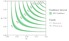
(a) Level curves with estimated confidence intervals for $n=100$ points per path.

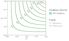
(b) Level curves with estimated confidence intervals for $n=10000$ points per path.

Figure 1: Level curves for the estimated copula with confidence intervals ($s=0.3$ and $t=0.7$).

In Figure 2 we report the finite-sample distribution of our standardized error against the standard normal distribution. We can see that the accuracy of our statistic is sensitive to the boundary points where $s$ and $t$ are close. Again, this behaviour is not unexpected; the temporal gradient $\nabla\psi$, as in Theorem 2, is given by

$$\begin{bmatrix}\int_{0}^{u}\varphi\left(\frac{\sqrt{t}\Phi^{-1}(v)-\sqrt{s}\Phi^{-1}(w)}{\sqrt{t-s}}\right)\left(\frac{\Phi^{-1}(v)}{2\sqrt{t(t-s)}}-\frac{\sqrt{t}\Phi^{-1}(v)-\sqrt{s}\Phi^{-1}(w)}{2\sqrt{t-s}^{3}}\right)dw\\ \\ \int_{0}^{u}\varphi\left(\frac{\sqrt{t}\Phi^{-1}(v)-\sqrt{s}\Phi^{-1}(w)}{\sqrt{t-s}}\right)\left(\frac{\sqrt{t}\Phi^{-1}(v)-\sqrt{s}\Phi^{-1}(w)}{2\sqrt{t-s}^{3}}-\frac{\Phi^{-1}(w)}{2\sqrt{s(t-s)}}\right)dw\end{bmatrix}.$$

Here, $\varphi$ is the density function of a standard Gaussian. We see, that terms proportional to $1/\sqrt{t-s}$ appear. However, recall that as $(s,t)\to(t_{0},t_{0})$ for $t_{0}>0$ the copula reduces to $C(t_{0},t_{0};u,v)=u\land v$. Furthermore, it is also very likely that numerical errors influence the result here, due to terms such as $1/\sqrt{t-s}$.

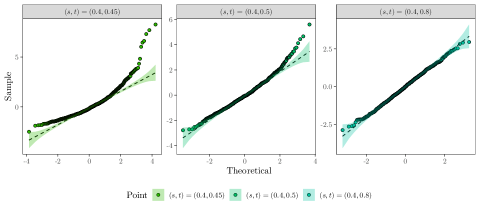
Figure 2: QQ plot for $\sqrt{n/V^{n}_{s,t}}\cdot(C^{n}(s,t;u,v)-C(s,t;u,v))$, $(n=10000,(u,v)=(0.7,0.3))$.

We conclude this section by investigating whether the convergence in Theorem 1 can be extended to uniform convergence over $(u,v)$. Specifically, we investigate, via Monte Carlo simulations, the asymptotic behavior of the statistic

$$\rho(C^{n},C):=\sup_{\begin{subarray}{c}(u,v)\in[0,1]^{2}\\ \tau\leq s,t\leq\mathscr{T}\end{subarray}}|C^{n}(s,t;u,v)-C(s,t;u,v)|,$$

as the sample size increases.

Figure 3: Density estimates for $\rho(C^{n},C)$ on a logarithmic scale.

Figure 3 shows the density estimates, obtained via a Gaussian kernel density estimate, for $\rho(C^{n},C)$ on a logarithmic scale focusing on the peaks. Observe that the mean is located in the lower tail, due to a substantial number of simulations resulting in $\rho(C^{n},C)$ being very close $0$. Similarly, $1/\sqrt{n}$ is also added to the plot, showing that the shift in the distribution is, relatively, proportional to $1/\sqrt{n}$ on a logarithmic scale. Based on Figure 3, these simulations indicate that Theorem 1 may be extended to include the supremum over $(u,v)\in[0,1]^{2}$.

4 Proofs

The following lemmas are key for the proof of our main results.

Lemma 1.

Let $\psi$ be as in (2.4). For all $u,v\in[0,1]$, the mapping $(s,t)\mapsto\psi(s,t;u,v)$ is continuous in $(0,\infty)^{2}$ and continuously differentiable in $\{(s,t)\mid 0<s<t\}$.

Proof.

If $(u,v)$ is in the boundary of $[0,1]^{2}$ the result is trivial. Suppose that $u,v\in(0,1)$ and put

$$g(t,s,w):=\Phi\left(\frac{\sqrt{t\lor s}\Phi^{-1}(v)-\sqrt{t\land s}\Phi^{-1}(w)}{\sqrt{\left|t-s\right|}}\right),\,\,\,t,s>0,w\neq v,$$

and $g(t,s,w)\equiv 0$ when $w=v$. From Example 5.32 in [13], it follows that for almost all $w\in[0,u]$

$$\lim_{(t,s)\rightarrow(t_{0},s_{0})}g(t,s,w)=\begin{cases}\mathbbm{1}_{[0,v]}(w)&\text{if }t_{0}=s_{0};\\ g(t_{0},s_{0},w)&\text{if }t_{0}\neq s_{0}.\end{cases}$$ (4.1)

The continuity then follows by the Lebesgue’s Dominated Convergence Theorem. On the other hand, for $w\neq v$ we have that for $0<s<t$

$$\begin{bmatrix}\dfrac{\partial g(s,t,w)}{\partial t}\\ \\ \dfrac{\partial g(s,t,w)}{\partial s}\end{bmatrix}=\begin{bmatrix}\varphi\left(\frac{\sqrt{t}\Phi^{-1}(v)-\sqrt{s}\Phi^{-1}(w)}{\sqrt{t-s}}\right)\left(\frac{\Phi^{-1}(v)}{2\sqrt{t(t-s)}}-\frac{\sqrt{t}\Phi^{-1}(v)-\sqrt{s}\Phi^{-1}(w)}{2\sqrt{t-s}^{3}}\right)\\ \\ \varphi\left(\frac{\sqrt{t}\Phi^{-1}(v)-\sqrt{s}\Phi^{-1}(w)}{\sqrt{t-s}}\right)\left(\frac{\sqrt{t}\Phi^{-1}(v)-\sqrt{s}\Phi^{-1}(w)}{2\sqrt{t-s}^{3}}-\frac{\Phi^{-1}(w)}{2\sqrt{s(t-s)}}\right)\end{bmatrix},$$

where $\varphi$ is density of a standard normal distribution. Since for any constants $c,k$ such that $k\neq 0$, it holds that $\varphi(c+kx)x\rightarrow 0$ as $\left|x\right|\rightarrow\infty$, we deduce that

$$\sup_{w\in[0,1]}\left\|\left(\dfrac{\partial g(s,t,w)}{\partial t},\dfrac{\partial g(s,t,w)}{\partial s}\right)\right\|<\infty,\,\,\,0<s<t.$$ (4.2)

Interchanging roles between $s$ and $t$ allow us to conclude that (4.2) is fulfilled for all $(s,t)\in\{(s,t)\mid 0<s<t\}$. Another application of the Dominated Convergence Theorem concludes the proof.∎

For the next result we need the following subspace of $\mathbb{D}([0,\mathscr{T}];\mathbb{R})$:

$$\mathbb{F}([0,\mathscr{T}];(0,\infty)=\mathbb{D}([0,\mathscr{T}];\mathbb{R})\cap\{f:[0,\mathscr{T}]\to(0,\infty)\mid f\text{ is non-decreasing}\}.$$

Lemma 2.

Let $g\in C((0,\infty)^{n};\mathbb{R}^{m}))$, $m,n\in\mathbb{N}$ and $\mathscr{T}>0$. Then the mapping

$$\Psi :(\mathbb{F}([0,\mathscr{T}];\mathbb{R})^{n},d_{\infty}^{n})\to(\mathbb{D}([0,\mathscr{T}]^{n};\mathbb{R}^{m}),d_{\infty})$$

$$x \mapsto g(x_{1}(t_{1}),x_{2}(t_{2}),\dots,x_{n}(t_{n})),\quad\forall t=(t_{1},t_{2},\dots,t_{n})\in[0,\mathscr{T}]^{n},$$

is continuous, where $d_{\infty}$ denotes the supremum metric.

Proof.

We must show, that for every $x=(x_{1},\ldots,x_{n})\in\mathbb{F}([0,\mathscr{T}];\mathbb{R})^{n}$ and $\varepsilon>0$ there exists a $\delta>0$ such that

$$d_{\infty}^{n}(x,y)<\delta\implies d_{\infty}(\Psi(x),\Psi(y))<\varepsilon.$$ (4.3)

To this end, note first that for all $i=1,\ldots,n$, $\inf_{t\in[0,\mathscr{T}]}x_{i}(t)=x_{i}(0)>0.$ Now, let $i=1,\ldots,n$ and consider the set $B_{x_{i}}=\{z\in\mathbb{F}([0,\mathscr{T}];\mathbb{R})\mid d_{\infty}(x_{i},y)\leq x_{i}(0)/2\}$. For $z\in B_{x_{i}}$ we have

$$|\sup_{t\in[0,\mathscr{T}]}\left|x_{i}(t)\right|-\sup_{t\in[0,\mathscr{T}]}\left|z(t)\right||=\sup_{t\in[0,\mathscr{T}]}\left|x_{i}(t)-z(t)\right|<\max_{i}x_{i}(0)/2=:c_{x_{i}}$$

This implies $\sup_{t\in[0,\mathscr{T}]}\left|z(t)\right|\leq\sup_{t\in[0,\mathscr{T}]}\left|x_{i}(t)\right|+c_{x_{i}}<\infty$. Now set $C_{x_{i}}=c_{x_{i}}+\sup_{t\in[0,\mathscr{T}]}x_{i}(t)$. Then, $z(t),x_{i}(t)\in[c_{x_{i}},C_{x_{i}}]$ for every $t\in[0,\mathscr{T}]$. Let $K=\prod_{i=1}^{n}[c_{x_{i}},C_{x_{i}}]\subset(0,\infty)^{n}$. By the Heine-Cantor Theorem, it follows that the restriction of $g$ to $K$ is uniformly continuous. This means that we can find $\delta_{0}>0$ such that for all $|t-s|<\delta_{0}\implies|g(t)-g(s)|<\varepsilon$. Now, put $\delta=\min(\delta_{0},c_{x_{1}},\ldots,c_{x_{n}})$. We conclude from above that if $y=(y_{1},\ldots,y_{n})\in\mathbb{F}([0,\mathscr{T}];\mathbb{R})^{n}$ and $d_{\infty}^{n}(x,y)<\delta$ then $x(t),y(t)\in K$ for all $0\leq t\leq\mathscr{T}$, from which (4.3) follows. ∎

Proof of Theorem 1.

Let $\mathscr{T}>t_{0}$. From Lemma 1, the mapping $(s,t)\mapsto\psi(s,t;u,v)$ is continuous in $(0,\infty)^{2}$. Thus, we deduce that $\psi$ extends (as in Lemma 2) to a continuous function $\Psi:\mathbb{F}([0,\mathscr{T}-t_{0}];(0,\infty)^{2})\to\mathbb{D}([0,\mathscr{T}]^{2};\mathbb{R})$. Moreover

$$C^{n}(\cdot,\cdot;u,v)=\Psi((S_{t_{0}}[X]^{n},S_{t_{0}}[X]^{n})));\,\,\,C(\cdot,\cdot;u,v)=\Psi(S_{t_{0}}T,S_{t_{0}}T),$$

where $S_{t_{0}}:\mathbb{D}([0,\mathscr{T}];\mathbb{R})\to\mathbb{D}([0,\mathscr{T}-t_{0}];\mathbb{R})$ denotes the shift operator, i.e.

$$x \mapsto(S_{t_{0}}x)(t)=x(t+t_{0}),\quad\forall t\in[0,\mathscr{T}-t_{0}].$$

In view that $S_{t_{0}}$ is a continuous operator from $\mathbb{D}([0,\mathscr{T}];\mathbb{R})$ to $\mathbb{D}([0,\mathscr{T}-t_{0}];\mathbb{R})$ and $[X]^{n}\overset{u.c.p}{\Rightarrow}T$, as $n\rightarrow\infty$, we can now apply The Continuous Mapping Theorem (see for instance [3]) to conclude that

$$d_{\infty}(\Psi(S_{t_{0}}[X]^{n},S_{t_{0}}[X]^{n}),\Psi(S_{t_{0}}T,S_{t_{0}}T))\overset{\mathbb{P}}{\rightarrow}0,$$

which is exactly the conclusion of the theorem.∎

Proof of Theorem 2.

First note that thanks to Lemma 5.3.12 in [8] we may and do assume that $\left|\sigma_{t}\right|\leq C$ for some deterministic constant $C>0$. Now, let

$$Z_{n}:=\left([X]^{n}_{t},[X]^{n}_{s}\right);\,\,\,Z:=\left(T_{t},T_{s}\right).$$

Since $\mathbb{P}(\sigma_{t}^{2}>0)=1$ for all $t\geq 0,$ we can find $n$ large enough such that $Z_{n}\in\{(s,t):0<s,t,t\neq s\}$. Moreover, by Taylor’s Theorem

$$\sqrt{n}\left[C^{n}(s,t;u,v)-C(s,t;u,v),\right]=\int_{0}^{1}\nabla\psi(Z+y(Z_{n}-Z),u,v)dy\cdot\sqrt{n}(Z_{n}-Z).$$

From Theorem 5.4.2 in [8], it follows that for any $s\neq t$

$$\sqrt{n}(Z_{n}-Z)\xrightarrow{s.d}\sqrt{2}\left(\int_{0}^{t}\sigma_{r}^{2}dW^{\prime}_{r},\int_{0}^{s}\sigma_{r}^{2}dW^{\prime}_{r}\right),$$

where $W^{\prime}$ is a Brownian motion independent of $\mathcal{F}$. Therefore, it is enough to show that

$$\int_{0}^{1}\nabla\psi(Z+y(Z_{n}-Z),u,v)dy\xrightarrow{\mathbb{P}}\nabla\psi\left(T_{t},T_{s},u,v\right).$$ (4.4)

In view that $Z_{n}\overset{\mathbb{P}}{\rightarrow}Z$, every subsequence $Z_{n_{k}}$ contains a further subsequence $Z_{n_{k(i)}}$ such that $Z_{n_{k(i)}}\xrightarrow{a.s.}Z$. Fix $\omega\in\Omega_{t,s}:=\{\omega\in\Omega:Z_{n_{k(i)}}(\omega)\rightarrow Z(\omega),Z(\omega)\in\{(s,t)\mid 0<s<t\}\}.$ By using that $Z(\omega)\in V$, we can find an open ball with center $Z(\omega)$ and radius $\rho(\omega)>0$ which is totally contained in $\{(s,t)\mid 0<s<t\}$. Moreover, for every $\rho>\varepsilon>0$ there is $n_{0}\equiv n_{0}(\omega)\in\mathbb{N}$ such that

$$\left\|Z_{n_{k(i)}}(\omega)-Z(\omega)\right\|<\varepsilon,\,\,\,\forall\,n_{k(i)}\geq n_{0}.$$

This in particular implies that for all $0\leq y\leq 1$ and $n_{k(i)}\geq n_{0}$, $Z(\omega)+y(Z_{n_{k(i)}}(\omega)-Z(\omega))$ is contained in an open ball with center $Z(\omega)$ and radius $\varepsilon>0$. Therefore, we can find a compact set $K_{\omega}\subseteq\{(s,t)\mid 0<s<t\}$ such that $Z(\omega)+y(Z_{n_{k(i)}}(\omega)-Z(\omega))\in K_{\omega}$ for all $0\leq y\leq 1$ and $n_{k(i)}\geq n_{0}$. Hence, by the continuity of $\nabla\psi$ on $\{(s,t)\mid 0<s<t\}$ (see Lemma 1) and the Dominated Convergence Theorem, we deduce that as $n_{k(i)}\rightarrow\infty$

$$\int_{0}^{1}\nabla\psi(Z(\omega)+y(Z_{n_{k(i)}}(\omega)-Z(\omega));u,v)dy\rightarrow\nabla\psi(Z(\omega);u,v),\,\,\forall\omega\in\Omega_{t,s}.$$

(4.4) follows now by Theorem 6.3.1 in [10].∎

References

- [1] O. E Barndorff-Nielsen and A. Shiryaev. Change of Time and Change of Measure. WORLD SCIENTIFIC, 2nd edition, 2015.
- [2] Xiaohong Chen and Yanqin Fan. Estimation of copula-based semiparametric time series models. Journal of Econometrics, 130(2):307–335, 2006.
- [3] U. Cherubini, F. Gobbi, S. Mulinacci, and S. Romagnoli. Introduction to empirical processes and semiparametric inference. John Wiley & Sons Ltd, 2012.
- [4] William F Darsow, Bao Nguyen, Elwood T Olsen, et al. Copulas and markov processes. Illinois journal of mathematics, 36(4):600–642, 1992.
- [5] Christian Genest, Michel Gendron, and Michaël Bourdeau-Brien. The advent of copulas in finance. The European Journal of Finance, 15(7-8):609–618, 2009.
- [6] Christian Genest, Kilani Ghoudi, and L-P Rivest. A semiparametric estimation procedure of dependence parameters in multivariate families of distributions. Biometrika, 82(3):543–552, 1995.
- [7] Erich Häusler and Harald Luschgy. Stable convergence and stable limit theorems, volume 74. Springer, 2015.
- [8] Jean Jacod and Philip Protter. Discretization of processes, volume 67. Springer Science & Business Media, 2011.
- [9] Andrew J Patton. Modelling asymmetric exchange rate dependence. International economic review, 47(2):527–556, 2006.
- [10] Sidney Resnick. A probability path. Springer, 2019.
- [11] G Salvadori and Carlo De Michele. On the use of copulas in hydrology: theory and practice. Journal of Hydrologic Engineering, 12(4):369–380, 2007.
- [12] Olivier Scaillet and Jean-David Fermanian. Nonparametric estimation of copulas for time series. FAME Research paper, (57), 2002.
- [13] Volker Schmitz. Copulas and stochastic processes. PhD thesis, Bibliothek der RWTH Aachen, 2003.
- [14] Andrew G Wilson and Zoubin Ghahramani. Copula processes. pages 2460–2468, 2010.
- [15] SC Yang, TJ Liu, and HP Hong. Reliability of tower and tower-line systems under spatiotemporally varying wind or earthquake loads. Journal of Structural Engineering, 143(10):04017137, 2017.