Stochastic Stability of Agglomeration Patterns in an Urban Retail Model

Abstract

We consider a model of urban spatial structure proposed by Harris and Wilson (Environment and Planning A, 1978). The model consists of fast dynamics, which represent spatial interactions between locations by the entropy-maximizing principle, and slow dynamics, which represent the evolution of the spatial distribution of local factors that facilitate such spatial interactions. One known limitation of the Harris and Wilson model is that it can have multiple locally stable equilibria, leading to a dependence of predictions on the initial state. To overcome this, we employ equilibrium refinement by stochastic stability. We build on the fact that the model is a large-population potential game and that stochastically stable states in a potential game correspond to global potential maximizers. Unlike local stability under deterministic dynamics, the stochastic stability approach allows a unique and unambiguous prediction for urban spatial configurations. We show that, in the most likely spatial configuration, the number of retail agglomerations decreases either when shopping costs for consumers decrease or when the strength of agglomerative effects increases.

Keywords: retail agglomeration; spatial interaction; multiple equilibria; local stability; stochastic stability.

JEL Classification: C62, R12, R13, R14

1 Introduction

Effective urban planning require a good understanding of how cities and regions change and grow over time. It is one of the central problems for contemporary science to understand the structure, function, and dynamics of cities. The key features of cities include activities at locations, flow patterns between these locations, and the internal spatial structure that facilitates these activities. To model such systems, Wilson, (2007) proposed the Boltzmann–Lotka–Volterra (BLV) method. The BLV method is a synthesis of fast dynamics (the “Boltzmann” component) and slow dynamics (the “Lotka–Volterra” component). Fast dynamics describe the short-run spatial interaction patterns (i.e., the flows between locations, such as trip distributions between the origin and destination pairs) and the short-run payoff landscape. Slow dynamics describe the gradual evolution of the spatial distribution of mobile factors that govern the processes of flow generation and attraction (i.e., the stocks at the locations, such as trip demand at the origins and attractiveness of the destinations). The fast dynamics of flow-based spatial interactions follow the entropy-maximizing framework (Wilson, , 1967, 1970). The BLV formalism adds slow dynamics by considering flow-dependent evolution of stock values at the locations. This combination of short- and long-run dynamics was being followed in new economic geography synthesized by Fujita et al., (1999) and, ultimately, to the recent wave of quantitative spatial models in economics surveyed by Redding and Rossi-Hansberg, (2017).

The prototype of the BLV method is the Harris and Wilson, (1978) (HW) model, a pioneering work in modeling the spontaneous formation of retail agglomerations in an urban area. Based on the static shopping models of Huff, (1963) and Lakshmanan and Hansen, (1965), Harris and Wilson formulated a dynamic model of spatial structure with agglomeration force. Their study illustrates that such a model can exhibit multiple equilibria, path dependence, and catastrophic phase transitions. Although their study considered the formation of retail agglomerations in an urban area as an application, the HW model, and more generally the BLV methodology, has a wider scope of applications, including logistics (Leonardi, 1981a, ; Leonardi, 1981b, ), archaeology (Bevan and Wilson, , 2013; Paliou and Bevan, , 2016), healthcare (Tang et al., , 2017), and crime (Davies et al., , 2013; Baudains et al., , 2016) to name a few (see Dearden and Wilson, , 2015, for an exposition on applications of the BLV method ). In light of these diverse applications, it is essential to have a solid understanding of the analytical aspects of the HW model.

One key issue of the HW model is that it converges to one of the multiple equilibria, depending on the initial conditions. The early explorations of the analytical properties of the model mainly focused on two-location settings for tractability (for example, Clarke, , 1981; Wilson, , 1981; Rijk and Vorst, 1983a, ; Rijk and Vorst, 1983b, ). However, they had already suggested that multiple locally stable equilibria could arise. Thereafter, extensive numerical simulations of the HW model in many-location settings has demonstrated that many locally stable equilibria can arise (Clarke and Wilson, , 1983, 1985; Wilson and Dearden, , 2011; Dearden and Wilson, , 2015). Further, by using an analytical method developed by Akamatsu et al., (2012), Osawa et al., (2017) formally illustrated that the model allows multiple locally stable states in many-location settings. The existence of multiple locally stable states means that the model’s prediction can be elusive and raises the question of robustness regarding the numerical findings in the literature.

To overcome this, we introduce a new approach that allows unambiguous prediction of the most likely spatial configuration in the HW model. We use the stochastic stability approach developed in game theory. We first show that the HW model is a potential game (Monderer and Shapley, , 1996; Sandholm, , 2001, 2009). In potential games, it is known that the set of global potential maximizers is stochastically stable. By global maximization of the potential function, we can determine the most likely spatial agglomeration patterns at each given value of the structural parameters of the model. This contrasts with the local stability approach in the literature, which exhibits multiple stable equilibria. We apply the stochastic stability approach to a two-dimensional square economy and show that, in the most likely spatial configuration, the number of retail agglomerations decreases either when shopping costs for consumers decrease or when the strength of agglomerative effects increases. These results corroborate the numerical findings in the literature.

The rest of this paper is organized as follows. Section 2 discusses our contribution to the literature. Section 3 introduces the HW model. Section 4 provides formal examples to demonstrate that the HW model can allow numerous locally stable equilibria simultaneously. Section 5 shows that the HW model is a potential game. Section 6 reviews the stochastic stability approach employed in this paper and provides a simple example. Section 7 applies the stochastic stability approach to the HW model in a two-dimensional economy. Section 8 concludes the paper.

2 Related literature

Harris and Wilson, (1978) showed that their model reduces to reduces to a maximization problem of a scalar-valued function with respect to spatial interaction patterns and spatial distribution of retailers. Consequently, we can interpret the HW model as a large-population potential game (Sandholm, , 2001, 2009), which, in turn, allows us to apply a stochastic stability approach developed in game theory literature in a simplified manner. Specifically, the stationary distribution of stochastic evolutionary dynamics in a potential game often becomes a Boltzmann–Gibbs measure that assigns a higher probability at a spatial configuration achieving a higher value of the potential. Stochastic stability considers some limits of stationary distribution, for example, the “low-temperature” limit, whereby the distribution concentrates on the unique set of global maximizers of the potential function (Blume, , 1993, 1997). Thus, this approach regards the global potential maximizers as stochastically stable states. We employ Sandholm, (2010)’s results on the limiting behaviors of the stationary distribution when the number of players grows to infinity, and noise level diminishes (the “double limits”). See Wallace and Young, (2015) for a survey of stochastic stability approaches in game theory.

One successful application of stochastic stability and potential games in the urban spatial context is Schelling, (1971)’s celebrated model of segregation, where a finite number of agents choose their locations on a discrete grid. Schelling’s studies demonstrate that a slight microscopic homophily can lead to macroscopic separation of two groups of people. By considering several specific functional forms for an individual’s utility function, Zhang, 2004a ; Zhang, 2004b ; Zhang, (2011) showed that potential functions can be used to characterize the equilibria of the model. Building on Zhang’s work, Grauwin et al., (2012) formulated Schelling’s model as a spatial evolutionary game and provided a general analysis using a potential game method. Zhang, 2004a ; Zhang, 2004b ; Zhang, (2011) and Grauwin et al., (2012) considered games with a finite number of agents and the limiting behavior of the stationary measure of stochastic dynamics when stochasticity diminishes—the small noise limit (Foster and Young, , 1990; Kandori et al., , 1993). To study the HW model where there is a continuum of agents, we build on Sandholm, (2010), Section 12, and consider double limits where the number of agents tends to infinity, and the level of noise diminishes.

Although the stochastic stability approach used in this study implicitly considers stochastic evolutionary dynamics, its predictions are deterministic because it considers the limiting behavior of the Boltzmann–Gibbs measure. One can instead directly study the behavior of the stochastic differential equation (SDE) obtained from the HW model. For example, Vorst, (1985) considered an SDE version of the HW model and defined a different type of stochastic stability concept, showing that equilibrium in the model is globally absorbing when it is unique. Compared with that, our approach can treat cases in which the model features multiple equilibria that are locally stable under deterministic dynamics. More recently, Ellam et al., (2018) proposed a unified approach based on an SDE formulation for the HW model to incorporate uncertainty and provided a Bayesian method for parameter estimation. They exploit the existence of a potential function for the HW model to facilitate analysis because the Boltzmann–Gibbs stationary distribution associated with their SDE formulation forms an integral part of the data-generating process for parameter estimation. Our approach instead focuses on the limiting behavior of the invariant measure to obtain cleaner theoretical insights into the agglomeration behavior of the HW model.

We contribute to the literature on potential game methods in spatial economic models. One example is the formation of central business districts as a result of agents’ social preference for proximity to others, as considered by Beckmann, (1976) and revisited by Mossay and Picard, (2011). By generalizing Mossay and Picard, (2011)’s framework with Beckmann-type social externalities, Blanchet et al., (2016) provided a variational (potential maximization) formulation for a general class of urban spatial models with a continuum of agents in continuous space. Stability characterization in such continuous-space models is difficult, although some authors have tackled this problem (for example, Bragard and Mossay, , 2016). Instead, by considering discrete-space versions of Beckmann-type models, Akamatsu et al., (2017) provided a potential function that can be used to characterize the stability of equilibria through more elementary means of finite-strategy evolutionary dynamics (as surveyed by Sandholm, , 2010). Similarly, Osawa and Akamatsu, (2020) showed that Fujita and Ogawa, (1982)’s seminal urban economics model on the formation of multiple business districts in a city is an instance of potential games when formulated in discrete space; global maximization of the potential function is also an effective method of analysis in this model. We expect that the discrete-space approach can provide a tractable strategy to continuous-space models, including variants of Schelling’s framework with a continuum of agents and continuous space (instead of discrete agents and discrete space), such as the model by Mossay and Picard, (2019).

3 An urban retail model

We briefly review the HW model following the version of Osawa et al., (2017). Consider a city comprising $K\in\mathbb{Z}$ discrete zones, where $\mathbb{Z}$ is the set of integers. Let $[K]\equiv\{1,2,\ldots,K\}$ denote the set of zones. There is a large continuum of retailers that can enter or exit any zone in the city, and the equilibrium mass of retailers in the city is given by an equilibrium condition. The spatial distribution of retailers is denoted by $\bm{x}=(x_{i})_{i\in[K]}$, where $x_{i}\geq 0$ is the mass of retailers in zone $i\in[K]$. We call $i\in[K]$ with $x_{i}>0$ a retail agglomeration. The spatial distribution of the retailers, $\bm{x}$, is the endogenous variable of the model.

There is a continuum of consumers whose spatial distribution is exogenously given. Each infinitesimal consumer purchases a fixed amount of goods sold by retailers. Consumers’ shopping behavior is modeled by a set of origin-constrained gravity equations, which is originally derived from the entropy-maximization principle (Wilson, , 1967), a foundation for the logit model. The value spent in zone $i$ by consumers from zone $j$ is

$$V_{ij}(\bm{x})=\frac{x_{i}^{\alpha}\exp\left(-\beta t_{ji}\right)}{\sum_{k\in[K]}x_{k}^{\alpha}\exp\left(-\beta t_{jk}\right)}Q_{j},$$ (3.1)

where the fixed constant $Q_{j}>0$ denotes total demand in zone $j$; $t_{ji}$ is the generalized travel cost from zone $j$ to $i$; $\alpha>0$ denotes scale economies; and $\beta>0$ represents the rate at which demand decreases in distance. All variables, except retailers’ spatial distribution $\bm{x}$, are exogenous. In HW’s terminology, $x_{i}^{\alpha}$ represents the attractiveness of zone $i$ for consumers.

Retailers incur a fixed cost $\kappa>0$ to enter a zone. The total revenue of zone $i$ is equally distributed among the retailers therein. The profit of a retailer in zone $i$, which is a function of $\bm{x}$, is then given by the following equation:

$$\pi_{i}(\bm{x}) \equiv\frac{1}{x_{i}}\sum_{j\in[K]}V_{ij}(\bm{x})-\kappa=\sum_{j\in[K]}\frac{x_{i}^{\alpha-1}\phi_{ji}}{\sum_{k\in[K]}x_{k}^{\alpha}\phi_{jk}}Q_{j}-\kappa,$$ (3.2)

where $\phi_{ij}\equiv\exp\left(-\beta t_{ij}\right)\in(0,1]$. We denote $\mathbf{D}\equiv[\phi_{ij}]_{ij\in[K]\times[K]}$ and $\bm{\pi}(\bm{x})\equiv(\pi_{i}(\bm{x}))_{i\in[K]}$. The fixed cost $\kappa$ can be assumed to be different across locations. As such an assumption changes only the scale of $x_{i}$, we assume $\kappa_{i}=\kappa$ for simplicity.

Equilibrium spatial distribution of retailers is determined by their entry–exit behavior. We assume that retailers enter zone $i$ if $\pi_{i}(\bm{x})>0$, exit if $\pi_{i}(\bm{x})<0$, and $x_{i}$ does not change if $\pi_{i}(\bm{x})=0$. That is, $x_{i}>0$ implies $\pi_{i}(\bm{x})=0$, and $\pi_{i}(\bm{x})=0$ implies $x_{i}\geq 0$; thus, retailers in all zones achieve zero profit in equilibrium. In addition, $x_{i}=0$ implies $\pi_{i}(\bm{x})\leq 0$; there is no incentive for retailers to relocate to or enter zones without retailers. This is represented by the following complementarity condition:

$$x_{i}\pi_{i}(\bm{x})=0,\ x_{i}\geq 0,\ \pi_{i}(\bm{x})\leq 0 \forall i\in[K].$$ (3.3)

Spatial equilibrium in the model is defined as follows.

Definition 1.

A state $\bm{x}\geq\bm{0}$ is a spatial equilibrium if it satisfies (3.3).

Following the literature, we investigate the evolution in spatial equilibrium patterns when there are changes in the structural parameters of the model. In particular, we focus on the roles of $\alpha$ and $\beta$.

Remark 1.

At any spatial equilibrium of the model, it must be that $\sum_{i\in[K]}x_{i}\pi_{i}(\bm{x})=0$; that is, $\sum_{i\in[K]}Q_{i}=\kappa\sum_{i\in[K]}x_{i}$. The left-hand side is the retailers’ total revenue, whereas the right-hand side is their total cost. Together with positivity $\bm{x}\geq\bm{0}$, this implies that any spatial equilibrium must lie in the following closed and convex set (Harris and Wilson, , 1978):

$$\mathcal{X}\equiv\left\{\bm{x}\geq\bm{0}\mathrel{}\middle|\mathrel{}\kappa\textstyle{\sum_{i\in[K]}}x_{i}=Q\right\},$$ (3.4)

where $Q\equiv\sum_{i\in[K]}Q_{i}$. Thus, $\sum_{i\in[K]}x_{i}=\frac{Q}{\kappa}$ at any spatial equilibrium. Without loss of generality, we assume $\frac{Q}{\kappa}=1$ for normalization, and $\mathcal{X}$ becomes the $(K-1)$-simplex. ∎

4 Multiplicity of locally stable equilibria

It is known that the HW model admits numerous spatial equilibria simultaneously. For example, Rijk and Vorst, 1983b showed that there are at least $\binom{K}{K/2}+1$ positive spatial equilibria when $K$ is even. To obtain realistic outcomes, the literature focuses on locally stable equilibria under deterministic adjustment dynamics, that is, the “slow dynamics” of the BLV method, which is defined as follows:

$$\dot{x}_{i}=E_{i}(\bm{x})\equiv x_{i}\pi_{i}(\bm{x})=\sum_{j\in[K]}\frac{x_{i}^{\alpha}\phi_{ji}}{\sum_{k\in[K]}x_{k}^{\alpha}\phi_{jk}}Q_{j}-\kappa x_{i}.$$ (D)

This is consistent with the equilibrium condition (3.3) in the sense that any stationary point of (D) is a spatial equilibrium. As an evolutionary dynamic on $\mathcal{X}$, (D) is a special case of the replicator dynamic (Taylor and Jonker, , 1978), where the average payoff is always zero.

Under (D), $\mathcal{X}$ is globally attracting in $\mathbb{R}_{+}^{N}$. The total mass of retailers increases if $Q>\kappa\sum_{i\in[K]}x_{i}$ and decreases if $Q<\kappa\sum_{i\in[K]}x_{i}$ because

$$\sum_{i\in[K]}\dot{x}_{i}=\sum_{i\in[K]}E_{i}(\bm{x})=\sum_{i\in[K]}x_{i}\pi_{i}(\bm{x})=Q-\kappa\sum_{i\in[K]}x_{i}.$$ (4.1)

Thus, we can focus on the states in $\mathcal{X}$ without loss of generality.

Equilibrium refinement based on local stability under (D) can leave numerous equilibria as locally stable states. For example, the mono-centric concentration of retailers in any single zone is always locally stable when $\alpha>1$.

Proposition 1.

Suppose $\alpha>1$. Then, a full concentration of retailers in a single zone, namely $x_{i}=\frac{Q}{\kappa}=1$ and $x_{j}=0$ ($j\neq i$) for some $i\in[K]$, is a locally stable spatial equilibrium for any $\mathbf{D}=[\phi_{ij}]$.

Proof.

If $x_{i}^{*}=1$ and $x_{j}^{*}=0$ ($j\neq i$), then it is a strict equilibrium because $\pi_{i}(\bm{x}^{*})=0>-\kappa=\pi_{j}(\bm{x}^{*})$ ($j\neq i$) if $\alpha>1$. Thus, it is locally stable under a wide range of dynamics, including (D) (Sandholm, , 2014). ∎

There is (at least) as many stable equilibria as the number of zones at any level of travel costs for consumers when $\alpha>1$. Further, the following result from Osawa et al., (2017) concretely demonstrates that nontrivial spatial patterns with more than two retail agglomerations can become locally stable simultaneously.

Proposition 2.

Suppose $\alpha>1$. Consider a one-dimensional circular economy, where $\phi_{ij}=\phi^{\ell_{ij}}$ with $\phi\in(0,1)$ and $\ell_{ij}=\min\{|i-j|,K-|i-j|\}$. Assume $K=2^{J}$ with $J\geq 3$. When $\phi$ and $\alpha$ are sufficiently small, all spatial patterns of the form

$$\bm{x}^{(k)}\equiv(\underbrace{\underbrace{2^{k}\bar{x},0,0,\ldots,0}_{\text{$2^{k}$ elements}},\underbrace{2^{k}\bar{x},0,0,\ldots,0}_{\text{$2^{k}$ elements}},\ldots,\underbrace{2^{k}\bar{x},0,0,\ldots,0}_{\text{$2^{k}$ elements}}}_{\text{repeated $K/2^{k}=2^{J-k}$ times}})$$ (4.2)

with $0\leq k\leq J$ and $\bar{x}=\frac{1}{K}$, up to symmetry, are locally stable simultaneously.

Proof.

See Osawa et al., (2017), Proposition 4. Their Figure 8 demonstrates this result numerically. ∎

If $\bm{x}^{(k)}$ ($k\geq 2$) is locally stable, then all $\bm{x}^{(l)}$ ($l\geq k$) are locally stable. For the case of $K=2^{4}=16$, Figure 1 shows the circular economy and spatial patterns $\{\bm{x}^{(k)}\}_{1\leq k\leq J}$. Further, notably spatial patterns other than $\{\bm{x}^{(k)}\}_{1\leq k\leq J}$ can be locally stable simultaneously.

(a) $K=2^{4}$ circle

(b) $\bm{x}^{(0)}=\bar{\bm{x}}$

(c) $\bm{x}^{(1)}$

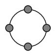
(d) $\bm{x}^{(2)}$

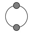
(e) $\bm{x}^{(3)}$

(f) $\bm{x}^{(4)}$

Figure 1: Circular economy and symmetric spatial configurations that can be simultaneously locally stable. Gray disks indicate the masses of retailers in the populated zones or retail agglomeration.

As these examples demonstrate that the equilibrium refinement based on local stability can leave multiple equilibria. We will also numerically illustrate this issue in Sections 6.2 and 7. To alleviate this, we introduce a new approach to equilibrium refinement, namely, an approach based on stochastic stability.

5 Potential game representation

For preparation, here, we observe that the HW model is a large-population potential game. Large-population games are defined as follows (see, for example, Sandholm, , 2010, for a survey).

Definition 2 (Large-population game).

Consider a game played by a continuum of homogeneous agents. Let $[S]=\{1,2,\ldots,S\}$ be the set of strategies, where $S\in\mathbb{Z}$ is the number of strategies. Let $\mathcal{Y}\equiv\{\bm{y}\in\mathbb{R}_{+}^{S}\mid\sum_{i\in[S]}y_{i}=1\}$ be the set of all possible strategy distributions, where $\mathbb{R}_{+}$ is the set of nonnegative reals, and $y_{i}\in[0,1]$ is the share of agents that play strategy $i\in[S]$. Let $\mathbf{F}:\mathcal{Y}\to\mathbb{R}^{S}$ be the Lipshitz continuous payoff function, whose $i$th component $F_{i}:\mathcal{Y}\to\mathbb{R}$ maps a state $\bm{y}\in\mathcal{Y}$ to payoff $F_{i}(\bm{y})$ for agents playing $i\in[S]$ at state $\bm{y}$. The tuple $([S],\mathbf{F})$ is called a large-population game.

We follow the convention, where $\mathbf{F}$ is defined over an open neighborhood of $\mathcal{Y}$ so that its differential is well-defined on $\mathcal{Y}$. The HW model can be seen as a large-population game $([K],\bm{\pi})$, where the set of retailers’ strategies is $[K]$, and their payoff function is $\bm{\pi}$. As we know that $\mathcal{X}$ contains all equilibria of the model, we can focus on the states in $\mathcal{X}$.

A large-population game whose payoff function is integrable is called a large-population potential game (Sandholm, , 2001, 2009).

Definition 3 (Large-population potential game).

A large population game $([S],\mathbf{F})$ is a potential game if there is a scalar-valued function $f$ defined in the neighborhood of $\mathcal{Y}=\{\bm{y}\in\mathbb{R}_{+}^{S}\mid\sum_{i\in[S]}y_{i}=1\}$ that satisfies $\frac{\partial f(\bm{y})}{\partial y_{i}}=F_{i}(\bm{y})$ for all $i\in[S]$ and $\bm{y}\in\mathcal{Y}$.

Subsequently, the next observation follows.

Observation 1.

The HW model is a large-population potential game. ∎

The following function $f:\mathbb{R}_{+}^{N}\to\mathbb{R}$ is the potential function for the payoff function $\bm{\pi}$:

$$f(\bm{x})\equiv\frac{1}{\alpha}\sum_{j\in[K]}Q_{j}\log\left(\sum_{k\in[K]}x_{k}^{\alpha}\phi_{jk}\right)-\kappa\sum_{i\in[K]}x_{i},$$ (P)

as we have $\nabla f(\bm{x})=\bm{\pi}(\bm{x})$ for all $\bm{x}\in\mathbb{R}_{+}^{K}$. The first term represents the accessibility for consumers, whereas the second term the total cost for retailers.

As all spatial equilibria of the HW model are contained in $\mathcal{X}$, the equilibria of the HW model, and their properties are characterized by the following potential maximization problem.

$$\max_{\bm{x}\in\mathcal{X}}.\ f(\bm{x}).$$ (PM)

First, the first-order necessary condition for the extrema (the Karush-Kuhn-Tucker condition) is equivalent to the equilibrium condition (3.3). Second, the set of local maximizers coincides with that of locally stable states under various deterministic dynamics, including (D). For example, it is stable under the best response dynamic (Gilboa and Matsui, , 1991), the Smith dynamic (Smith, , 1984), the Brown-von Neumann-Nash dynamic (Brown and von Neumann, , 1950; Nash, , 1951), and a class of Riemannian game dynamics (Mertikopoulos and Sandholm, , 2018) that encompasses the projection dynamic (Dupuis and Nagurney, , 1993) as a special case.

Remark 2.

If $\alpha\in(0,1)$, then we can show that $f$ is strictly convex, and thus, (PM) has a unique global maximizer. This fact provides a simple proof for the uniqueness of equilibrium in the HW model when $\alpha\in(0,1)$, which was originally shown by Theorem 2 of Rijk and Vorst, 1983a or Theorem 1 of Vorst, (1985). Vorst, (1985) notes that (P) is a Lyapunov function for (D) when $\alpha\in(0,1)$. In addition, in light of the potential function $f$, Proposition 1 has another interpretation. Every corner of $\mathcal{X}$ corresponds to the full concentration of retailers in a zone. Each of them is a local maximizer for the problem (PM) if $\alpha>1$, and hence locally stable. ∎

Remark 3.

As $\sum_{i\in[K]}x_{i}^{*}=\sum_{i\in[K]}x_{i}^{**}=\frac{Q}{\kappa}=1$ for any two equilibria $\bm{x}^{*}$ and $\bm{x}^{**}$ in $\mathcal{X}$, we have $f(\bm{x}^{*})-f(\bm{x}^{**})=g(\bm{x}^{*})-g(\bm{x}^{**})$, where $g$ is the first term of $f$ in (P), which corresponds to a welfare measure for immobile consumers in terms of the aggregate accessibility to retail agglomerations (Harris and Wilson, , 1978; Leonardi, , 1978). It is a log-sum function commonly used in transport research, which was initially suggested by Williams, (1977) (see de Jong et al., , 2007, for a recent survey). For the HW model, it corresponds to the social aggregate of the expected maximum utility of immobile consumers under the logit model, where, concretely, a consumer in $i\in[K]$ chooses their shopping destination $j\in[K]$ by maximizing the random utility of the form $u_{ij}=\alpha\log x_{j}-\beta t_{ij}+\epsilon$ with $\epsilon$ being i.i.d. Gumbel. The larger the equilibrium potential value, the greater the accessibility to retail agglomerations for immobile consumers in equilibrium. ∎

6 A stochastic stability approach for equilibrium refinement

6.1 Stochastic relocation, stochastic stability, and potential function

As we have seen in Section 4, equilibrium refinement based on local stability under deterministic dynamics can result in inconclusive predictions in the context of the HW model. To overcome this, we employ a stronger equilibrium refinement based on stochastic stability given the existence of a potential function. Sandholm, (2010), Sections 11.5 and 12.2 develop a theory under which the global maximizers of the potential function are stochastically stable. We briefly review the essence of his analysis. See Wallace and Young, (2015) for a broader survey on stochastic stability approaches in game theory.

To define the stochastic stability of a state, we introduce the stochastic relocation dynamics of retailers. For this, we regard the HW model as a continuous (or large-population) and deterministic limit of a discrete (or atomic) and stochastic analog of the model.

Suppose there is a finite (but large) number of retailers, instead of a continuum, and let $N\in\mathbb{Z}$ be the finite number of retailers. Then, a strategy distribution (spatial distribution) of finite retailers can be seen as an element of the discrete set $\mathcal{X}^{N}\subset\mathcal{X}$ defined by $\mathcal{X}^{N}\equiv\left\{\bm{x}\in\mathcal{X}\mathrel{}\middle|\mathrel{}N\bm{x}\in\mathbb{Z}^{K}\right\}$. For $\bm{x}\in\mathcal{X}^{N}$, we have $x_{i}\in\{0,\frac{1}{N},\frac{2}{N},\ldots,\frac{N-1}{N},1\}$.

Every retailer receives strategy revision opportunities (i.e., it may exit a zone and then enter another) according to a Poisson process with a unit rate. When a retailer in zone $i$ receives a revision opportunity at state $\bm{x}\in\mathcal{X}^{N}$, it switches from zone $i$ to $j\neq i$ according to the following logit rule.

$$\rho_{j}(\bm{x})=\dfrac{\exp\left(\eta^{-1}\pi_{j}(\bm{x})\right)}{\sum_{k\in[K]}\exp\left(\eta^{-1}\pi_{k}(\bm{x})\right)},$$ (6.1)

where $\eta>0$. We have $\rho_{j}(\bm{x})>\rho_{k}(\bm{x})$ if $\pi_{j}(\bm{x})>\pi_{k}(\bm{x})$, meaning that retailers prefer locations with higher profit. The parameter $\eta$ can be interpreted as the level of noise in retailers’ choice, as $\eta\to 0$ implies that every retailer switches to $j$ with the highest profit with probability $1$. If $\eta$ is high, retailers could make suboptimal choices and relocate to less profitable zones than their current choice. This rule may represent errors in retailers’ decisions or unobservable heterogeneities of retailers.

These behavioral assumptions induce a stochastic dynamic for retailers’ spatial distribution or a Markov process $\{\mathbf{X}_{t}^{N}\}$ on the discrete state space $\mathcal{X}^{N}$. It has a common jump rate $N$, and the transition probabilities from state $\bm{x}\in\mathcal{X}^{N}$ to $\bm{y}\in\mathcal{X}^{N}$ are as follows.

$$P_{\bm{x}\to\bm{y}}^{N}=\begin{cases}x_{i}\rho_{j}(\bm{x})&\text{if }\bm{y}=\bm{x}+\tfrac{1}{N}(\bm{e}_{j}-\bm{e}_{i}),\ j\neq i\\ \sum_{i\in[K]}x_{i}\rho_{i}(\bm{x})&\text{if }\bm{y}=\bm{x},\\ 0&\text{otherwise},\end{cases}$$ (6.2)

where $\bm{e}_{i}$ is the $i$th standard basis in $\mathbb{R}^{K}$. Under this stochastic evolutionary law, the state can move only to neighboring states in $\mathcal{X}^{N}$.

Sandholm, (2010), Theorem 11.5.12 shows that the Markov process $\{\mathbf{X}_{t}^{N}\}$ admits a unique stationary distribution $\mu^{N,\eta}$ on $\mathcal{X}^{N}$ as follows.

$$\mu^{N,\eta}(\bm{x})=\frac{1}{Z}\frac{N!}{\prod_{k\in[K]}(Nx_{k})!}\exp\left(\eta^{-1}f^{N}(\bm{x})\right),$$ (6.3)

where $Z>0$ is the normalizing constant that ensures that $\sum_{\bm{x}\in\mathcal{X}^{N}}\mu^{N,\eta}(\bm{x})=1$; the function $f^{N}:\mathcal{X}^{N}\to\mathbb{R}$ is a discrete analog for the potential function $f$ for the large-population case, whose details are irrelevant for our purpose. We require only that $\{\frac{1}{N}f^{N}\}$ converges uniformly to $f$ as $N\to\infty$.

In evolutionary game theory, a state is said to be stochastically stable when the stationary distribution of a stochastic dynamic assigns a positive weight on the state in some limits of the structural parameters of the dynamic adjustment process. One leading example is stochastic stability in the small noise limit (Foster and Young, , 1990; Kandori et al., , 1993). A state $\bm{x}^{*}\in\mathcal{X}^{N}$ is stochastically stable in the small noise limit when

$$\lim_{\eta\to 0}\mu^{N,\eta}(\bm{x})>0.$$ (6.4)

In the limit $\eta\to 0$, retailers choose zones with higher profit with higher probability. The small noise limit is, thus, a deterministic limit where noise vanishes and retailers recover optimal choice behavior.

Small noise limit can be understood with the formula (6.3). We have

$$\frac{\mu^{N,\eta}(\bm{x})}{\mu^{N,\eta}(\bm{y})}=\underbrace{\frac{\prod_{k\in[K]}(Ny_{k})!}{\prod_{k\in[K]}(Nx_{k})!}}_{\text{constant in $\eta$}.}\exp\left(\eta^{-1}\left(f^{N}(\bm{x})-f^{N}(\bm{y})\right)\right)$$ (6.5)

for two states $\bm{x},\bm{y}\in\mathcal{X}^{N}$. If $f^{N}(\bm{x})-f^{N}(\bm{y})>0$, then the right-hand side grows infinitely large as $\eta\to 0$. That is, $\mu^{N,\eta}$ assigns higher and higher probability on the states with larger values of $f^{N}$ when $\eta$ goes smaller and smaller. In the limit, $\mu^{N,\eta}$ concentrates on the states that globally maximize $f^{N}$. Thus, the global maximizers of discrete potential $f^{N}$ are stochastically stable in the small noise limit under a fixed $N$.

In a similar spirit to the small noise limit, the double limits considers a situation where $N\to\infty$ and $\eta\to 0$. By taking these two limits, we recover our model as laid out in Section 3, in which retailers do not incur errors, and the set of retailers is a continuum. Thus, stochastic stability in double limits provides a refinement procedure for the deterministic large-population model. We employ the following result for the double limits.

Fact 1 (Sandholm, (2010), Corollary 12.2.5).

The stationary distribution $\mu^{N,\eta}$ concentrates on global maximizers of the potential function $f$ in the double limits; that is, the set of global maximizers in a potential game is stochastically stable in the double limits. ∎

6.2 Applying stochastic stability

Stochastic stability provides stronger refinement for spatial equilibria than local stability, as the latter corresponds to looking at local maximizers of $f$. Simply put, we look into the properties of global maximizers for the problem (PM). To apply the refinement based on stochastic stability, the following procedure is carried out.

1. Fix parameters $\bm{\theta}\in\Theta$, where $\Theta$ is the feasible set of the structural parameters of interest. Enumerate all spatial patterns $\bm{x}^{*1}(\bm{\theta})$, $\bm{x}^{*2}(\bm{\theta})$, $\bm{x}^{*3}(\bm{\theta})$, $\ldots$ that can be local maximizers of the potential function, and let $\mathcal{E}(\bm{\theta})\equiv\{\bm{x}^{*1}(\bm{\theta}),\bm{x}^{*2}(\bm{\theta}),\bm{x}^{*3}(\bm{\theta}),\ldots\}\subset\mathcal{X}$.

2. Select the global potential maximizers of potential $f(\cdot,\bm{\theta})$ by the comparison of the potential values for the candidate equilibrium patterns in $\mathcal{E}(\bm{\theta})$.

3. By moving $\bm{\theta}$ throughout $\Theta$ and repeating the two steps above, obtain the partition of $\Theta$ based on the global potential maximizer.

The main structural parameters of the model are $\alpha$ and $\beta$ because we assume that the underlying geographical environment for retailers (i.e., $\{t_{ij}\}$ and $\{Q_{j}\}$) is exogenous, and we normalize $\frac{Q}{\kappa}=1$. By definition, the set of local potential maximizers $\mathcal{E}(\bm{\theta})$ contains all global potential maximizers at $\bm{\theta}$ because a stochastically stable state $\bm{x}^{*}$ for a given $\bm{\theta}$ must satisfy $\bm{x}^{*}\in\operatornamewithlimits{arg\,max}_{\bm{x}\in\mathcal{E}(\bm{\theta})}f(\bm{x},\bm{\theta})$. By exhausting all possible $\bm{\theta}$ in the parameter space $\Theta$, we can obtain its partition based on stochastic stability, which provides basic insights into the implication of the model.

Below, we consider an illustrative example. Suppose a symmetric two-zone city; let $K=2$, $t_{11}=t_{22}=0$, $t_{12}=t_{21}=1$, and $Q_{1}=Q_{2}=\frac{\kappa}{2}$ so that $\frac{Q}{\kappa}=1$. We fix $\alpha$ and consider the changes of $\beta$. For completeness of the diagrams, we use

$$\phi\equiv\exp\left(-\beta\right)\in(0,1),$$ (6.6)

which is the level of freeness of consumers’ inter-zone travel. For $\alpha$, we let $\alpha=1.2$. We note that the preferred estimate for $\alpha$ available in the literature is $1.18$, which is obtained by applying the model to the London retail system (Ellam et al., , 2018).

Figure 2 shows the bifurcation diagram of spatial equilibria along the $\phi$ axis in terms of $x_{1}$. Figure 2(a) considers local stability of equilibria under (D). The black solid curves show locally stable equilibria, whereas the gray dashed curves represent locally unstable equilibria. As the two zones are symmetric, the uniform distribution of retailers $\bar{\bm{x}}=\left(\frac{1}{2},\frac{1}{2}\right)$ across zones is always a spatial equilibrium. It is stable for small $\phi$ and becomes locally unstable at $\phi^{*}=\frac{1-\sqrt{\bar{\alpha}}}{1+\sqrt{\bar{\alpha}}}$ with $\bar{\alpha}\equiv\frac{\alpha-1}{\alpha}$ (Osawa et al., , 2017, Proposition 1). If retailers are initially distributed uniformly, then it is stable when $\phi$ is small, and a steady increase in $\phi$ induces the spontaneous formation of retail agglomeration at $\phi^{*}$. The only equilibria that can be stable are $\bar{\bm{x}}$ and the full concentration $\bm{x}^{*1}\equiv(1,0)$ and $\bm{x}^{*2}\equiv(0,1)$ (or simply, agglomeration of retailers in either zone). Agglomeration is locally stable for all $\phi$, in accordance with Proposition 1. All three equilibria are stable when $\phi\in(0,\phi^{*})$; there are no criteria to further select one (or two). However, when $\phi\in(0,0.2)$, Figure 2(a) suggests that the region of attraction for agglomeration is infinitesimally small. This indicates that a very small perturbation is sufficient to nudge the equilibrium toward dispersion when $\phi$ is small. In this respect, agglomeration is “less relevant” when $\phi$ is small.

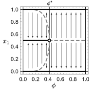
(a) Local stability

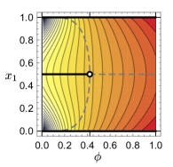
(b) Contour of $f$

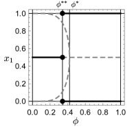
(c) Stochastic stability

Figure 2: Local stability and stochastic stability of equilibria in a two-zone symmetric city ($\alpha=1.2$, $\phi\equiv\exp\left(-\beta\right)$). Panel(a): The thin arrows indicate direction of adjustment under dynamic (D). The solid black curves indicate locally stable equilibrium values of $x_{1}$. The dashed gray curves are locally unstable equilibria. Panel (b): Contours of space $f$ on $(\phi,x_{1})$ space. Red indicates a higher value of potential. Panel (c): Equilibrium refinement by stochastic stability. The black solid curves indicate stochastically stable equilibria.

Figure 2(b) shows contours of $f$ on $(\phi,x_{1})$ space, together with the curves of spatial equilibria in Figure 2(a). The paths of spatial equilibria trace the extrema of $f$. Locally stable equilibria are local maximizers, whereas locally unstable ones are either minimizers or saddle points. Thus, we let $\mathcal{E}(\phi)=\left\{\bar{\bm{x}},\bm{x}^{*1},\bm{x}^{*2}\right\}$ for all $\phi$ in Step 1.

Figure 2(c) is the bifurcation diagram obtained by global maximization of potential function in $\mathcal{E}(\phi)$ at each level of $\phi$ (i.e., Step 2) and then varying $\phi$ (i.e., Step 3). Formally, we conclude as follows.

Proposition 3.

Suppose $K=2$ and consider the symmetric case where $t_{11}=t_{22}=0$, $t_{12}=t_{21}=1$, and $Q_{1}=Q_{2}=\frac{\kappa}{2}$. Let $\phi^{**}\equiv\frac{1}{2}(4^{\alpha}-2-\sqrt{4^{\alpha}(4^{\alpha}-1)})$. Then, dispersion $\bm{x}=(\frac{1}{2},\frac{1}{2})$ is stochastically stable when $\phi\in(0,\phi^{**}]$, whereas agglomeration $\bm{x}=(1,0)$ or $\bm{x}=(0,1)$ is stochastically stable when $\phi\in[\phi^{**},1)$.

Proof.

For any $\alpha>1$, $\phi=\phi^{**}$ solves the equation $f(\bar{\bm{x}},\phi)=f(\bm{x}^{*1},\phi)$. The uniform distribution globally maximizes $f$ over $\mathcal{X}$ when $\phi\in(0,\phi^{**}]$, whereas agglomeration does so when $\phi\in[\phi^{**},1)$. ∎

By comparing Figure 2(a) and Figure 2(c), we see that the latter extracts the essential implication of the former by ignoring the “less relevant” local maximizers. Thus, stochastic stability provides a way of simplifying the bifurcation diagram while preserving the basic implications of the model.

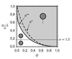
Figure 3: Stochastically stable states in a two-zone city ($\alpha\geq 1$). The black solid (dashed) curve indicates the threshold for stochastic stability of agglomeration (local stability of dispersion). Agglomeration is stochastically stable in the shaded region, whereas dispersion is stochastically stable. Under the myopic dynamics (D), dispersion is locally stable below the dashed curve, whereas agglomeration is always locally stable.

Figure 3 shows the partition of the parameter space based on Proposition 3. The case $\alpha\in(0,1)$ is omitted because the equilibrium is unique and stable if $\alpha\in(0,1)$ (Rijk and Vorst, 1983a, ). The boundary curve between the gray and white regions is $\phi^{**}$ in Proposition 3. Agglomeration is stochastically stable in the shaded region, whereas dispersion is stochastically stable in the blank region. The schematics show the stochastically stable spatial pattern in each region. Agglomeration tends to become stochastically stable when $\alpha$ is high and/or $\beta$ is low, that is, $\phi=\exp\left(-\beta\right)$ is high. The dashed curve indicates the threshold $\phi^{*}$ at which $\bar{\bm{x}}$ becomes locally unstable. Dispersion $\bar{\bm{x}}$ is locally stable below the dashed curve, whereas agglomeration is always locally stable. Figure 2 corresponds to a cross section of Figure 3 when $\alpha=1.2$.

7 Potential maximizing equilibria in two dimensions

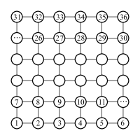
(a) Square economy

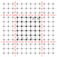
(b) Periodic boundary conditions

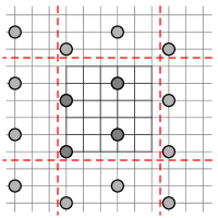
(c) An agglomeration pattern

Figure 4: $6\times 6$ square economy with periodic boundary conditions

The two-zone example demonstrates that the stochastic stability approach is effective for distilling the essential implications from the HW model. As a further illustration, we turn our attention to a two-dimensional space, which has been the focus of the model’s practical applications. We aim to obtain an analog of Figure 3 for two-dimensional settings.

A standard symmetric setting for theoretical investigation in regional science is an infinitely extended two-dimensional space as per the central place theory (Christaller, , 1933; Lösch, , 1940). As an analog of infinitely extended two-dimensional space, we consider a symmetric square economy with periodic boundaries.

Figure 4(a) shows the economy, where the sequentially numbered zones are indicated by circles; thin lines indicate the transportation network. The zones are equidistantly placed on a regular square network; the distance between each neighboring zone is one unit. We focus on the case $K=6\times 6=36$, which is the smallest square number that can be divided by both $2$ and $3$.

Figure 4(b) illustrates the periodic boundary conditions. For example, zone $1$ is neighboring not only to zones $2$ and $7$ but also to zones $6$ and $31$. As the figure shows, this economy can be regarded as an approximation of an infinitely extended two-dimensional space. Although we focus on the $K=36$ case, considering a higher $K$ does not qualitatively alter the results (Ikeda et al., , 2018, 2019).

Figure 4(c) shows, as an example of agglomeration patterns in this economy, a four-centric pattern where the gray disks schematically show retailers’ spatial distribution $\bm{x}$. A spatial configuration in a $6\times 6$ lattice can be seen as an infinitely repeated pattern on a two-dimensional space in this manner.

Let $\phi_{ij}=\phi^{\ell_{ij}}$ for all $i,j\in[K]$, where $\ell_{ij}\geq 0$ is the shortest path length between $i$ and $j$ and $\phi=\exp(-\beta)$. For example, $\ell_{1,2}=1$, $\ell_{1,9}=3$, $\ell_{1,36}=2$, and $\ell_{1,28}=5$. Alternatively, $\phi_{ij}=\exp(-\beta\ell_{ij})$. Consumer demand is assumed to be spatially uniform: $Q_{j}=\frac{Q}{K}$ for all $j\in[K]$. Based on these assumptions, we abstract away all the exogenous advantages induced by the underlying transport network and focus on the endogenous mechanisms in the HW model.

The difficulty of considering such many-zone settings lies in Step 1 of the procedure discussed in Section 6.2. An enumeration of all equilibria is practically impossible. To alleviate this, we use a systematic approach developed by Ikeda et al., (2018, 2019) to enumerate all the important candidates of spatial equilibria: invariant equilibria. Invariant equilibria are a special class of special equilibrium patterns in which all retail agglomerations (zones with retailers) host the same mass of retailers.

Definition 4.

A spatial equilibrium $\bm{x}^{*}\in\mathcal{X}$ is an invariant equilibrium if $x_{i}^{*}=\frac{1}{M}$ for all $i\in\operatorname{supp}(\bm{x}^{*})\equiv\{i\in[K]\mid x_{i}^{*}>0\}$, where $M=\left|{\operatorname{supp}(\bm{x}^{*})}\right|$ is the number of retail agglomerations.

For example, if $K=2$, as in Section 7, $\bar{\bm{x}}=\left(\frac{1}{2},\frac{1}{2}\right)$, $\bm{x}^{*1}=(1,0)$, and $\bm{x}^{*2}=(0,1)$ are invariant equilibria, and they exhaust all equilibrium patterns that can be locally stable. For the $6\times 6$ square economy considered in this section, there are $83$ invariant equilibria (see Figure 9 in Appendix B).

In any invariant equilibrium for a general $K$ zone economy with spatially uniform demand ($Q_{j}=Q/K$ for all $j\in[K]$), all retail agglomerations must be geographically symmetric in the sense that they have a common level of market share. To see this, consider a spatial pattern $\bm{x}^{*}$ in which retailers are located uniformly in $M\leq K$ zones. For $\bm{x}^{*}$ to satisfy the equilibrium condition $\pi_{i}(\bm{x}^{*})=0$, it must be

$$\sum_{j\in[K]}\frac{\phi_{ji}}{\sum_{k\in\operatorname{supp}(\bm{x}^{*})}\phi_{jk}}\frac{Q_{j}}{x_{i}^{*}}-\kappa=\sum_{j\in[K]}\frac{\phi_{ji}}{\Phi_{j}(\bm{x}^{*})}\frac{QM}{K}-\kappa=0 \forall i\in\operatorname{supp}(\bm{x}^{*}),$$ (7.1)

since $x_{i}^{*}=1/M$ for every $i\in\operatorname{supp}(\bm{x}^{*})$; $\Phi_{j}(\bm{x}^{*})=\sum_{k\in\operatorname{supp}(\bm{x}^{*})}\phi_{jk}$ is the aggregate accessibility from zone $j$ to the retail agglomerations. We note that $\bar{\phi}_{ji}\equiv\frac{\phi_{ji}}{\Phi_{j}(\bm{x}^{*})}$ is the share of shopping demand to $i$ in the total demand from $j$. Since $Q/\kappa=1$, we have

$$\sum_{j\in[K]}\bar{\phi}_{ji}\frac{1}{K}=\frac{1}{M}, \forall i\in\operatorname{supp}(\bm{x}^{*}).$$ (7.2)

The left-hand side is the aggregate market share of each retail agglomeration. Thus, (7.2) means that all retail agglomerations $i\in\operatorname{supp}(\bm{x}^{*})$ should face the same share of demand $\frac{1}{M}$, if retailers are located uniformly in $M$ locations.

In fact, all invariant equilibria exhibit geometric symmetry in which every retail agglomeration has the same level of market share in the square economy (see Figure 9 in Appendix B), thereby satisfying condition (7.2). Since changing $\phi$ uniformly and symmetrically reduces the accessibility between zones, all invariant equilibria are spatial equilibria for any value of $\phi$.

For any $K$, invariant equilibria in symmetric geographies can be identified using group theory. They are characterized by the group that represents the symmetry of the geography (Ikeda et al., , 2018). For example, when we consider a square lattice economy with $K=n^{2}$ locations and periodic boundaries, it can be formally shown that $M$ must divide $8K=8n^{2}$. In addition, invariant equilibrium can be enumerated by a computational group theory algorithm implemented by, for example, the GAP, (2019) software. Given the set of all invariant equilibria, we can consider the global maximization of the potential function $f$ over it.

In summary, the modified procedure we employ in this section is as follows.

1. Enumerate all invariant equilibria $\bar{\bm{x}}^{*1}$, $\bar{\bm{x}}^{*2}$, $\bar{\bm{x}}^{*3}$, $\ldots$, and let $\bar{\mathcal{E}}\equiv\{\bar{\bm{x}}^{*1},\bar{\bm{x}}^{*2},\bar{\bm{x}}^{*3},\ldots\}$.

2. At each value of structural parameters $\bm{\theta}\equiv\left(\alpha,\beta\right)$, select the global potential maximizer(s) of potential $f(\cdot,\bm{\theta})$ among the set of invariant equilibria $\bar{\mathcal{E}}$.

3. By moving $\bm{\theta}$ throughout $\Theta$ and repeating Step 2’, obtain the partition of $\Theta$ based on the global potential maximizer.

The set of invariant equilibria $\bar{\mathcal{E}}$ coincides exactly with that of all equilibria that can be a local potential maximizer if $K=2$. By definition, $\bar{\mathcal{E}}$ does not cover spatial equilibria in which there are retail agglomerations of different sizes. Therefore, $\bar{\mathcal{E}}$ may not exhaust all possible local potential maximizers in many-zone settings. However, we expect that they encompass all relevant patterns in symmetric geography. In fact, previous studies of spatial agglomeration models in symmetric many-location setups have suggested that most locally stable equilibria that emerge in line with monotonic changes are invariant equilibria (Ikeda et al., , 2018, 2019). It is also expected that symmetric spatial distributions, such as invariant equilibria, are natural candidates for global potential maximizers. Our assumption here is that the global maximization of potential in the set of invariant equilibria $\bar{\mathcal{E}}$ will provide a sufficiently accurate view of the overall properties of stochastically stable equilibria.

Figure 9 in Appendix B lists all the invariant equilibria in $6\times 6$ square economy (up to symmetry), which completes Step 1’. By conducting Step 3’ numerically, Figure 5 shows the partition of the $(\phi,\alpha)$ space based on the global potential maximizer in the same way as Figure 3. For example, the region with “D” in Figure 5(a) indicates that the duo-centric pattern in Figure 5(b) is the global potential maximizer among $\bar{\mathcal{E}}$ in that parametric region. Only $8$ among the $83$ invariant equilibria can be the global maximizers of the potential in $\bar{\mathcal{E}}$. When the freeness of interaction $\phi$ is low or returns to scale $\alpha$ are low, the retailers are spatially dispersed. As $\phi$ and $\alpha$ increase, the number of retail agglomerations decreases, and the spacing between them increases. As a robustness check, Appendix A compares the results for the square grid economy and a triangular grid economy. It is observed that the basic implications do not alter qualitatively.

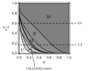
(a) Partition of the $(\phi,\alpha)$ space

Uniform (83)

18-centric (80)

12-centric (76)

8-centric (61)

6-centric (47)

Quad-centric (37)

Duo-centric (10)

Mono-centric (01)

(b) Stochastically stable patterns

Figure 5: Equilibrium selection based on global maximization of the potential function in a square lattice economy with $36$ locations ($\alpha\geq 1$). Panel (a) shows the partition of $(\phi,\alpha)$-space based stochastic stability, whereas Panel (b) shows the associated spatial configurations. The number in the label of each spatial configuration corresponds to Figure 9 in Appendix B. In Panel (a), the letters M, D, and Q indicate the mono-, duo-, and quad-centric equilibria, respectively; U indicates uniform equilibrium; the $\{18,12,8,6\}$-centric equilibrium patterns are sequentially aligned from the bottom left to the top right in the figure.

Equilibrium refinement based on global maximization of the potential function is by far sharper than that based on local stability (i.e., local maximization of potential). To demonstrate this, Figure 6 compares the local and global maximization of $f$. We consider $\alpha=1.2$ and $\alpha=2.5$, which are indicated in Figure 5 by the horizontal dashed lines. The vertical axis corresponds to $83$ invariant equilibria for the $6\times 6$ square economy. The lower the index of the spatial pattern, the lower the number of zones in which retailers locate. For example, pattern $83$ corresponds to the uniform distribution and pattern $01$, which corresponds to the full concentration in one of the zones (see Figure 9 in Appendix B). Each gray solid line indicates the range of $\phi$, in which the corresponding invariant equilibrium is a local maximizer of the potential function; that is, it is a locally stable equilibrium under (D). The black portion of each gray line, if any, indicates that the spatial configuration maximizes the potential function among all invariant equilibria. In Figures 6(a) and 6(b), the entire range of $\phi\in(0,1)$ is covered by locally stable invariant equilibria. This would indicate that invariant equilibria occupy essential parts of the set of all spatial equilibria and that other asymmetric equilibria are transient patterns of secondary importance, as is the case for other models of economic agglomeration (Ikeda et al., , 2018, 2019).

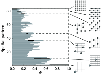
(a) $\alpha=1.2$

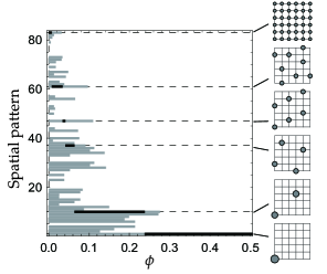
(b) $\alpha=2.5$

Figure 6: Comparison of refinement based on local stability and maximization of the potential function for $\alpha=1.2$ and $\alpha=2.5$. The vertical axis corresponds to the invariant patterns shown in Figure 9 in Appendix B. The solid lines indicate the range of $\phi$, in which the invariant equilibrium is locally stable under (D). The black portion on a gray solid line indicates that the equilibrium maximizes the potential value among the invariant equilibria in the range of $\phi$. Panels (a) and (b) correspond to the cross-sections indicated in Figure 5(a). In Panel (a), $8$ patterns can be the global maximizer, whereas $6$ patterns can be seen in Panel (b).

In Figure 6(a), $\alpha=1.2$, and the centripetal force is relatively weak. Figure 6(a) demonstrates that many configurations can become locally stable simultaneously. For example, when $\phi=0.1$, all the $83$ patterns are locally stable. Although retailers tend to agglomerate in a smaller number of locations when $\phi$ increases, the local stability approach creates ambiguity over which configuration is the most relevant outcome. Instead, by considering the global maximization of the potential function, we can single out only $8$ patterns (indicated by the horizontal dashed lines in Figure 6(a)) that can become the global maximizer of $f$ among the invariant patterns.

In Figure 6(b), we consider the case $\alpha=2.5$. As centripetal force is strong, multiple retail agglomerations tend to become unstable. Some invariant equilibria can never be locally stable when $\phi=0.1$. There is still the possibility of a multiplicity of locally stable equilibria. Global maximization of the potential function allows an unambiguous prediction at each level of $\phi$. Only $6$ invariant equilibria can globally maximize the potential function; compared with Figure 6(a), $18$- and $12$-centric patterns are skipped.

In sum, the basic implications of the HW model are that a decrease in transport costs (i.e., an increase in $\phi$) and an increase in centripetal force $\alpha$ promote retailers’ concentration in increasingly fewer locations. These results corroborate the numerical findings in the literature (e.g., Clarke and Wilson, , 1985; Dearden and Wilson, , 2015). As the previous numerical simulations in the literature are based on deterministic dynamics (D), the obtained equilibria can be one of many possibilities, as illustrated by Figure 6. Conversely, the stochastic stability approach pins down a unique prediction at each parameter value, providing a refined view of agglomeration behavior in the HW model.

8 Concluding remarks

The Harris and Wilson model is a parsimonious framework for the formation of urban spatial structures. This study introduces a new approach for equilibrium selection in the model based on the theory of stochastic evolutionary dynamics in potential games. We first observe that the model is an instance of large-population potential games and use a refinement of equilibrium by stochastic stability. Stochastic stability, or global maximization of a potential function, allows unambiguous prediction of the equilibrium spatial structure, unlike local stability. Our results provide a refined justification for previous numerical observations, which point out that lowering transport costs promotes concentration.

To enumerate all the important spatial configurations in two-dimensional settings, we used a group-theoretic approach developed by Ikeda et al., (2018, 2019) to consider the set of invariant equilibria. A similar approach to focus on symmetric patterns was adopted by Osawa and Akamatsu, (2020) in the context of an urban economics model. One technical limitation of this approach is that, by construction, we ignore asymmetric spatial configurations. However, we expect that the set of invariant equilibria has sufficient representativeness to capture the comparative statics of stochastically stable equilibrium configurations for our symmetric setup.

The simplicity of the Harris and Wilson framework allows its application in diverse contexts and enables researchers to develop a unified framework of parameter estimation. Some studies aim to deepen the physics of Wilson, (2007)’s BLV framework. For example, Crosato et al., (2018) considered the thermodynamic efficiency of urban transformation. In addition, in considering the long-run evolution of urban spatial structure, an important generalization is to consider the resettlement of consumers (Slavko et al., , 2019). This means that there are two types of qualitatively different actors in the model, in contrast to the original HW framework. Osawa and Akamatsu, (2020) showed that the potential maximization approach employed in this study could be an effective method of analysis for models with multiple types of agents. Further development of the potential game approach for modeling urban spatial structure would be profitable for both theory and applications.

Appendix A Triangular grid economy

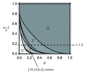
(a) Partition of the $(\phi,\alpha)$ space

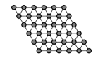
Uniform (65)

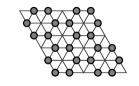
18-centric (63)

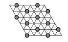
12-centric (57)

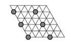
6-centric (33)

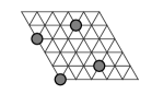
Quad-centric (25)

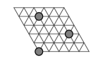
Tri-centric (14)

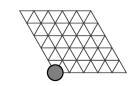
Mono-centric (01)

(b) Stochastically stable patterns

Figure 7: Equilibrium selection based on global maximization of the potential function in a triangular lattice economy with $36$ locations ($\alpha\geq 1$). Panel (a) shows the partition of $(\phi,\alpha)$-space based stochastic stability, whereas Panel (b) shows the associated spatial configurations. The number in the label of each spatial configuration corresponds to Figure 10 in Appendix B. In Panel (a), the letters M and T indicate the mono- and duo-centric equilibria, respectively; U indicates uniform equilibrium; the $\{18,12,6,4\}$-centric equilibrium patterns are sequentially aligned from left to right on the $\phi$ axis.

For a robustness check, we compare the square economy with another two-dimensional space, a symmetric triangular lattice economy, as considered by Ikeda and Murota, (2014). A triangular lattice economy with periodic boundaries is significant because the hexagonal market area envisaged by central place theory (Christaller, , 1933; Lösch, , 1940) can endogenously emerge as a locally stable equilibrium in general equilibrium models (Ikeda et al., , 2014, 2017). In the context of the HW model, Beaumont et al., (1981) provided a numerical investigation on a hexagonal economy with a triangular lattice. To compare the results with the square lattice case, we consider a $6\times 6$ triangular lattice economy with $6\times 6=36$ locations. In the triangular case, there are $65$ invariant equilibria, which we list in Figure 9 in Appendix B. Ikeda et al., (2019) provide a detailed discussion on the properties of invariant equilibria. For example, the number of retail agglomerations $M$ must divide $12n^{2}$. Only $7$ among the $65$ invariant equilibria can globally maximize the potential function.

Figure 7 shows the partition of $(\phi,\alpha)$ space based on the invariant equilibrium with the highest potential value. The partition is qualitatively similar to Figure 5. The spatial configurations are aligned from the bottom left to the top right according to the number of retail agglomerations. In addition to the uniform distribution and full agglomeration in a zone, there are two representative configurations that occupy relatively large regions in the parameter space: 12-centric and tri-centric patterns. The former corresponds to Christaller’s $k=3$ system, as $\frac{36}{12}=3$. Both the patterns feature hexagonal market area considered in central place theory.

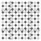
18-centric

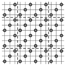
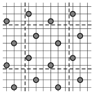
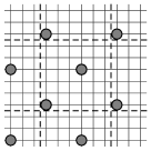
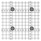
$\to$ 12-centric $\to$ Quad-centric $\to$ Duo-centric $\to$ Mono-centric

(a) Square lattice

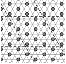
12-centric

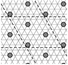
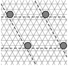
$\to$ Tri-centric $\to$ Mono-centric

(b) Triangular lattice

Figure 8: Comparison of evolution of the potential-maximizing spatial structure in the square and triangular lattices. Representative patterns are shown for the $\alpha=1.2$ cross-section indicated in Figure 5 and Figure 7.

Figure 8 compares the evolution of potential-maximizing invariant equilibria in the square and triangular lattices. We consider a monotonic increase in $\phi$ in Figures 5 and 7 under $\alpha=1.2$. It can be seen that the basic implication is the same: as $\phi$ increases, the size of retail agglomeration grows, and the spacing between them widens.

Appendix B Invariant equilibria in two-dimensional economy

Figure 9 shows all invariant equilibria for the $6\times 6$ square economy with periodic boundaries. In these spatial patterns, retail agglomerations are symmetrically placed over the square economy. For example, in patterns $29$, $64$, and $80$, retail agglomerations are equidistantly placed to form square patterns. Figure 4(c) in the main text shows pattern 37.

Figure 10 shows all invariant equilibria for the $6\times 6$ triangular lattice economy with periodic boundaries. Analogous to Figure 9, retail agglomerations exhibit geographical symmetry.

In our stylized two-dimensional economy, these invariant equilibria are characterized by the group $G$ that represents the symmetry of the economy. For example, the square lattice with periodic boundaries is invariant (symmetric) under $90^{\circ}$, $180^{\circ}$, and $270^{\circ}$ rotation as well as horizontal and vertical translation; and $G$ is a mathematical object that encapsulates such symmetry. By exploiting this symmetry, the GAP software (GAP, , 2019) was employed to enumerate the invariant equilibria for the square and triangular lattice economy considered in this study. For each geography, we first enumerate all the subgroups $\{G^{\prime}\}$ in the ground group $G$. Subsequently, we apply orbit decomposition for each subgroup $G^{\prime}$, which is a partitioning of the set of locations $[K]$ into equivalence class defined by the action of $G^{\prime}$ (i.e., the permutations of zone indices induced by $G^{\prime}$). The support $\operatornamewithlimits{supp}(\bar{\bm{x}}^{*})$ of each invariant equilibria $\bar{\bm{x}}^{*}$ corresponds to one of the partitioned components of $[K]$. For details, see Ikeda et al., (2018) and Ikeda et al., (2019) that provide group-theoretic analysis of invariant equilibria in square and triangular economies, respectively, with an arbitrary number of locations.

​

Figure 9: The full list of invariant equilibria for a square grid economy with $6\times 6$ locations.

​

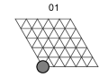
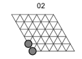
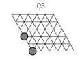
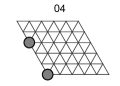
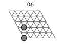
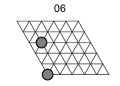
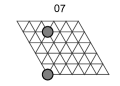
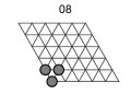
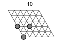
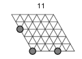
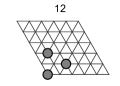
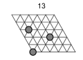
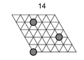
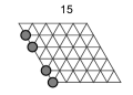
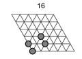
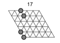
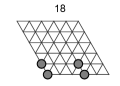
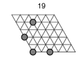
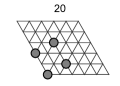
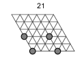
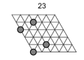
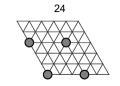
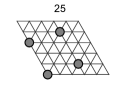
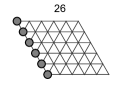
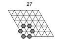
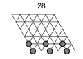
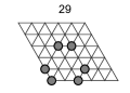
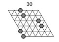
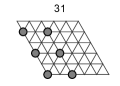
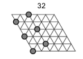
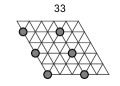
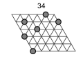
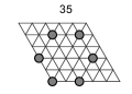
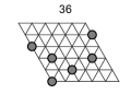
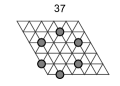
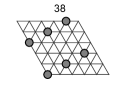
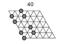
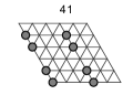
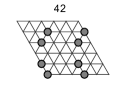
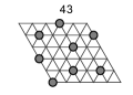
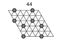
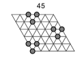
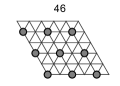
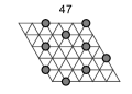
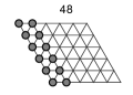
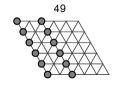
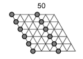
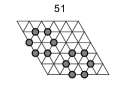
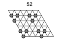
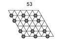
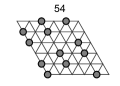
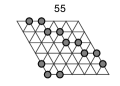
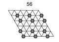
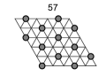
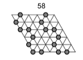
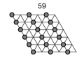
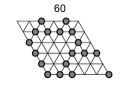
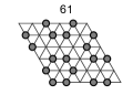
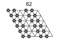
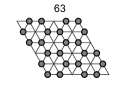
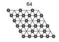
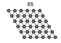
Figure 10: The full list of invariant equilibria for a triangular lattice economy with $6\times 6$ locations.

References

- Akamatsu et al., (2017) Akamatsu, T., Fujishima, S., and Takayama, Y. (2017). Discrete-space agglomeration models with social interactions: Multiplicity, stability, and continuous limit of equilibria. Journal of Mathematical Economics, 69:22–37.
- Akamatsu et al., (2012) Akamatsu, T., Takayama, Y., and Ikeda, K. (2012). Spatial discounting, fourier, and racetrack economy: A recipe for the analysis of spatial agglomeration models. Journal of Economic Dynamics and Control, 99(11):32–52.
- Baudains et al., (2016) Baudains, P., Fry, H. M., Davies, T. P., Wilson, A. G., and Bishop, S. (2016). A dynamic spatial model of conflict escalation. European Journal of Applied Mathematics, 27(3):530–553.
- Beaumont et al., (1981) Beaumont, J. R., Clarke, M., and Wilson, A. G. (1981). Changing energy parameters and the evolution of urban spatial structure. Regional Science and Urban Economics, 11(3):287–315.
- Beckmann, (1976) Beckmann, M. J. (1976). Spatial equilibrium in the dispersed city. In Environment, Regional Science and Interregional Modeling, pages 132–141. Springer.
- Bevan and Wilson, (2013) Bevan, A. and Wilson, A. (2013). Models of settlement hierarchy based on partial evidence. Journal of Archaeological Science, 40(5):2415–2427.
- Blanchet et al., (2016) Blanchet, A., Mossay, P., and Santambrogio, F. (2016). Existence and uniqueness of equilibrium for a spatial model of social interactions. International Economic Review, 57(1):36–60.
- Blume, (1993) Blume, L. E. (1993). The statistical mechanics of strategic interaction. Games and Economic Behavior, 5(3):387–424.
- Blume, (1997) Blume, L. E. (1997). Population games. The Economy as an Evolving Complex System II, 27:425–460.
- Bragard and Mossay, (2016) Bragard, J. and Mossay, P. (2016). Stability of a spatial model of social interactions. Chaos, Solitons & Fractals, 83:140–146.
- Brown and von Neumann, (1950) Brown, G. W. and von Neumann, J. (1950). Solutions of games by differential equations. In Kuhn, H. W. and Tucker, A. W., editors, Contributions to the Theory of Games I. Princeton University Press.
- Christaller, (1933) Christaller, W. (1933). Die Zentralen Orte in Süddeutschland. Gustav Fischer, Jena. (English translation: Central Places in Southern Germany, Prentice Hall, Englewood Cliffs, 1966).
- Clarke, (1981) Clarke, M. (1981). A note on the stability of equilibrium solutions of production-constrained spatial interaction models. Environment and Planning A, 13(5):601–604.
- Clarke and Wilson, (1983) Clarke, M. and Wilson, A. G. (1983). The dynamics of urban spatial structure: Progress and problems. Journal of Regional Science, 23(1):1–18.
- Clarke and Wilson, (1985) Clarke, M. and Wilson, A. G. (1985). The dynamics of urban spatial structure: the progress of a research programme. Transactions of the Institute of British Geographers, 10(4):427–451.
- Crosato et al., (2018) Crosato, E., Nigmatullin, R., and Prokopenko, M. (2018). On critical dynamics and thermodynamic efficiency of urban transformations. Royal Society Open Science, 5(10):180863.
- Davies et al., (2013) Davies, T. P., Fry, H. M., Wilson, A. G., and Bishop, S. R. (2013). A mathematical model of the london riots and their policing. Scientific reports, 3:1303.
- de Jong et al., (2007) de Jong, G., Daly, A., Pieters, M., and van der Hoorn, T. (2007). The logsum as an evaluation measure: Review of the literature and new results. Transportation Research Part A: Policy and Practice, 41(9):874–889.
- Dearden and Wilson, (2015) Dearden, J. and Wilson, A. G. (2015). Explorations in Urban and Regional Dynamics: A Case Study in Complexity Science. Routledge.
- Dupuis and Nagurney, (1993) Dupuis, P. and Nagurney, A. (1993). Dynamical systems and variational inequalities. Annals of Operations Research, 44(1):7–42.
- Ellam et al., (2018) Ellam, L., Girolami, M., Pavliotis, G. A., and Wilson, A. (2018). Stochastic modelling of urban structure. Proceedings of the Royal Society A: Mathematical, Physical and Engineering Sciences, 474(2213):20170700.
- Foster and Young, (1990) Foster, D. and Young, P. (1990). Stochastic evolutionary game dynamics. Theoretical Population Biology, 38(2):219–232.
- Fujita et al., (1999) Fujita, M., Krugman, P., and Venables, A. (1999). The Spatial Economy: Cities, Regions, and International Trade. Princeton University Press.
- Fujita and Ogawa, (1982) Fujita, M. and Ogawa, H. (1982). Multiple equilibria and structural transition of non-monocentric urban configurations. Regional Science and Urban Economics, 12:161–196.
- GAP, (2019) GAP (2019). GAP – Groups, Algorithms, and Programming, Version 4.10.2. The GAP Group.
- Gilboa and Matsui, (1991) Gilboa, I. and Matsui, A. (1991). Social stability and equilibrium. Econometrica, 59(3):859–867.
- Grauwin et al., (2012) Grauwin, S., Goffette-Nagot, F., and Jensen, P. (2012). Dynamic models of residential segregation: An analytical solution. Journal of Public Economics, 96(1-2):124–141.
- Harris and Wilson, (1978) Harris, B. and Wilson, A. G. (1978). Equilibrium values and dynamics of attractiveness terms in production-constrained spatial-interaction models. Environment and Planning A, 10(4):371–388.
- Huff, (1963) Huff, D. L. (1963). A probabilistic analysis of shopping center trade areas. Land Economics, 31(1):81–90.
- Ikeda et al., (2019) Ikeda, K., Kogure, Y., Aizawa, H., and Takayama, Y. (2019). Invariant patterns for replicator dynamics on a hexagonal lattice. International Journal of Bifurcation and Chaos, 29(06):1930014.
- Ikeda and Murota, (2014) Ikeda, K. and Murota, K. (2014). Bifurcation Theory for Hexagonal Agglomeration in Economic Geography. Springer.
- Ikeda et al., (2014) Ikeda, K., Murota, K., Akamatsu, T., Kono, T., and Takayama, Y. (2014). Self-organization of hexagonal agglomeration patterns in new economic geography models. Journal of Economic Behavior & Organization, 99:32–52.
- Ikeda et al., (2017) Ikeda, K., Murota, K., and Takayama, Y. (2017). Stable economic agglomeration patterns in two dimensions: Beyond the scope of central place theory. Journal of Regional Science, 57(1):132–172.
- Ikeda et al., (2018) Ikeda, K., Onda, M., and Takayama, Y. (2018). Spatial period doubling, invariant pattern, and break point in economic agglomeration in two dimensions. Journal of Economic Dynamics and Control, 29:129–152.
- Kandori et al., (1993) Kandori, M., Mailath, G. J., and Rob, R. (1993). Learning, mutation, and long run equilibria in games. Econometrica, pages 29–56.
- Lakshmanan and Hansen, (1965) Lakshmanan, J. and Hansen, W. G. (1965). A retail market potential model. Journal of the American Institute of Planners, 31(2):134–143.
- Leonardi, (1978) Leonardi, G. (1978). Optimum facility location by accessibility maximizing. Environment and Planning A, 10(11):1287–1305.
- (38) Leonardi, G. (1981a). A unifying framework for public facility location problems—part 1: A critical overview and some unsolved problems. Environment and Planning a, 13(8):1001–1028.
- (39) Leonardi, G. (1981b). A unifying framework for public facility location problems—part 2: Some new models and extensions. Environment and Planning a, 13(9):1085–1108.
- Lösch, (1940) Lösch, A. (1940). Die räumliche Ordnung der Wirtschaft. Gustav Fischer, Jena. (English translation: The Economics of Location, Yale University Press, 1954).
- Mertikopoulos and Sandholm, (2018) Mertikopoulos, P. and Sandholm, W. H. (2018). Riemannian game dynamics. Journal of Economic Theory, 177:315–364.
- Monderer and Shapley, (1996) Monderer, D. and Shapley, L. S. (1996). Potential games. Games and Economic Behavior, 14(1):124–143.
- Mossay and Picard, (2019) Mossay, P. and Picard, P. (2019). Spatial segregation and urban structure. Journal of Regional Science, 59(3):480–507.
- Mossay and Picard, (2011) Mossay, P. and Picard, P. M. (2011). On spatial equilibria in a social interaction model. Journal of Economic Theory, 146(6):2455–2477.
- Nash, (1951) Nash, J. (1951). Non-cooperative games. Annals of Mathematics, 54(2):286–295.
- Osawa and Akamatsu, (2020) Osawa, M. and Akamatsu, T. (2020). Equilibrium refinement for a model of non-monocentric internal structures of cities: A potential game approach. Journal of Economic Theory, 187:105025.
- Osawa et al., (2017) Osawa, M., Akamatsu, T., and Takayama, Y. (2017). Harris and wilson (1978) model revisited: The spatial period-doubling cascade in an urban retail model. Journal of Regional Science, 57(3):442–466.
- Paliou and Bevan, (2016) Paliou, E. and Bevan, A. (2016). Evolving settlement patterns, spatial interaction and the socio-political organisation of late prepalatial south-central crete. Journal of Anthropological Archaeology, 42:184–197.
- Redding and Rossi-Hansberg, (2017) Redding, S. J. and Rossi-Hansberg, E. (2017). Quantitative spatial economics. Annual Review of Economics, 9:21–58.
- (50) Rijk, F. and Vorst, A. (1983a). Equilibrium points in an urban retail model and their connection with dynamical systems. Regional Science and Urban Economics, 13(3):383–399.
- (51) Rijk, F. and Vorst, A. (1983b). On the uniqueness and existence of equilibrium points in an urban retail model. Environment and Planning A, 15(4):475–482.
- Sandholm, (2001) Sandholm, W. H. (2001). Potential games with continuous player sets. Journal of Economic Theory, 97(1):81–108.
- Sandholm, (2009) Sandholm, W. H. (2009). Large population potential games. Journal of Economic Theory, 144(4):1710–1725.
- Sandholm, (2010) Sandholm, W. H. (2010). Population Games and Evolutionary Dynamics. MIT Press.
- Sandholm, (2014) Sandholm, W. H. (2014). Local stability of strict equilibria under evolutionary game dynamics. Journal of Dynamics & Games, 1(3):485.
- Schelling, (1971) Schelling, T. C. (1971). Dynamic models of segregation. Journal of Mathematical Sociology, 1(2):143–186.
- Slavko et al., (2019) Slavko, B., Glavatskiy, K., and Prokopenko, M. (2019). Dynamic resettlement as a mechanism of phase transitions in urban configurations. Physical Review E, 99(4):042143.
- Smith, (1984) Smith, M. J. (1984). The stability of a dynamic model of traffic assignment: An application of a method of Lyapunov. Transportation Science, 18(3):245–252.
- Tang et al., (2017) Tang, J.-H., Chiu, Y.-H., Chiang, P.-H., Su, M.-D., and Chan, T.-C. (2017). A flow-based statistical model integrating spatial and nonspatial dimensions to measure healthcare access. Health & Place, 47:126–138.
- Taylor and Jonker, (1978) Taylor, P. D. and Jonker, L. B. (1978). Evolutionary stable strategies and game dynamics. Mathematical Biosciences, 40(1-2):145–156.
- Vorst, (1985) Vorst, T. (1985). A stochastic version of the urban retail model. Environment and Planning A, 17(12):1569–1580.
- Wallace and Young, (2015) Wallace, C. and Young, H. P. (2015). Stochastic evolutionary game dynamics. In Young, H. P. and Zamir, S., editors, Handbook of Game Theory with Economic Applications, volume 4, pages 327 – 380. Elsevier.
- Williams, (1977) Williams, H. C. (1977). On the formation of travel demand models and economic evaluation measures of user benefit. Environment and Planning A, 9(3):285–344.
- Wilson and Dearden, (2011) Wilson, A. and Dearden, J. (2011). Phase transitions and path dependence in urban evolution. Journal of Geographical Systems, 13(1):1–16.
- Wilson, (1967) Wilson, A. G. (1967). A statistical theory of spatial distribution models. Transportation research, 1(3):253–269.
- Wilson, (1970) Wilson, A. G. (1970). Entropy in Urban and Regional Modelling. Pion Ltd.
- Wilson, (1981) Wilson, A. G. (1981). Catastrophe Theory and Bifurcation: Applications to Urban and Regional Systems. University of California Press.
- Wilson, (2007) Wilson, A. G. (2007). Boltzmann, Lotka and Volterra and spatial structural evolution: An integrated methodology for some dynamical systems. Journal of the Royal Society Interface, 5(25):865–871.
- (69) Zhang, J. (2004a). A dynamic model of residential segregation. Journal of Mathematical Sociology, 28(3):147–170.
- (70) Zhang, J. (2004b). Residential segregation in an all-integrationist world. Journal of Economic Behavior & Organization, 54(4):533–550.
- Zhang, (2011) Zhang, J. (2011). Tipping and residential segregation: a unified schelling model. Journal of Regional Science, 51(1):167–193.