Appendix A More occlusion analysis
Here we perform more analysis on how the LSTM and matching loss enable ROLL to be robust to object occlusions. To analyze this, we generate a large number of puck moving trajectories in the Hurdle-Top Puck Pushing environment. Next, we train three different models on these trajectories:
-
•
LSTM with matching loss
-
•
LSTM without matching loss
-
•
object-VAE (with no LSTM).
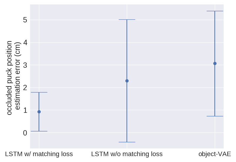
For each trajectory, we add synthetic occlusions to a randomly selected frame (by removing 85% of the pixels) and we use the three models to compute the latent encodings of the occluded frame (using the LSTM with the previous trajectory for models 1 and 2). We then use this embedding to retrieve the nearest neighbor frame in the collection of unoccluded trajectories whose latent embedding has the closest distance to the occluded latent embedding. This retrieved frame allows us to visualize the position that the model “thinks” the occluded puck is located at. For models 1 and 2, the model can use the LSTM and the previous trajectory to infer the location of the puck; for model 3, it cannot.
Finally, to evaluate this prediction, we compute the real puck distance between the location of the puck in the retrieved frame and the location of the puck in the occluded frame (using the simulator to obtain the true puck position, although this information is not available to the model). This distance can be interpreted as the estimation error of the puck position under occlusions. We report the mean and standard deviation of the estimation errors for three models in Supplementary Figure 1(a). As shown, using the LSTM + matching loss achieves the lowest average estimation error of roughly just 1cm, while LSTM without matching loss has a larger error of 2.2 cm and object-VAE has the largest error of 3.1 cm.
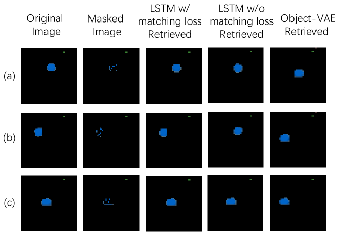
We can also visualize these retrievals, as shown in Supplementary Figure 2. We see that in all demonstrations, LSTM with matching loss almost perfectly retrieved the true unoccluded frames, while LSTM without matching loss and object-VAE retrieved incorrect frames with shifted puck positions. This shows that, even under severe occlusions (in the example, 85% of the pixels are dropped), with the LSTM and matching loss, ROLL can still correctly reason about the location of the object.
 |
 |
 |
 |
| (a) | (b) | (c) | (d) |
 |
 |
| (a) | (b) |
 |
 |
| (c) | (d) |
Appendix B More policy visualizations
Supplementary Figure 3 shows more policy visualizations of ROLL and Skew-Fit. We can see that in most cases, ROLL can achieves better manipulation results than Skew-Fit, aligning the object better with the target object position in the goal image. Skew-fit does not reason about objects and instead embeds the entire scene into a latent vector; further, Skew-fit does not reason about occlusions. Videos of the learned policies on all tasks are attached within the supplementary materials.
Appendix C Sensitivity on matching loss coefficient
We further test how sensitive ROLL is to the matching loss coefficient, on the Hurdle-Top Puck Pushing and the Hurdle-Bottom Puck Pushing task. The result is shown in Supplementary Figure 4. From the results we can see that ROLL is only sensitive to the VAE matching loss coefficient when the task has large occlusions, i.e., in the Hurdle-Top Puck Pushing task. We also observe that in this task, the larger the VAE matching loss coefficient, the better the learning results. ROLL is more robust to the VAE matching loss coefficient in the Hurdle-Bottom Puck Pushing task, and we observe that larger VAE matching loss coefficients lead to slightly worse learning results. This is because Hurdle-Bottom Puck Pushing task has a very small chance of object occlusions; thus too large of a VAE matching loss coefficient might instead slightly hurt the learned latent embedding. An intermediate VAE matching loss of 600 appears to perform well for both tasks. Additionally, we see that ROLL is quite robust to the LSTM matching loss coefficient in both tasks.
Appendix D Details on unknown object segmentation
We now detail how we train the background subtraction module and the robot segmentation network in unknown object segmentation.
To obtain a background subtraction module, we cause the robot to perform random actions in an environment that is object free, and we record images during this movement. We then train a background subtraction module using the recorded images. Specifically, we use the Gaussian Mixture-based Background/Foreground Segmentation algorithm [GMM_bg_subtraction1, GMM_bg_subtraction2] implemented in OpenCV [opencv_library]. In more detail, we use BackgroundSubtractorMOG2 implemented in OpenCV. We record 2000 images of the robot randomly moving in the scene, set the tracking history of BackgroundSubtractorMOG2 to 2000, and then train it on these images with an automatically chosen learning rate and variance threshold implemented by OpenCV. The background subtraction module is fixed after this training procedure.
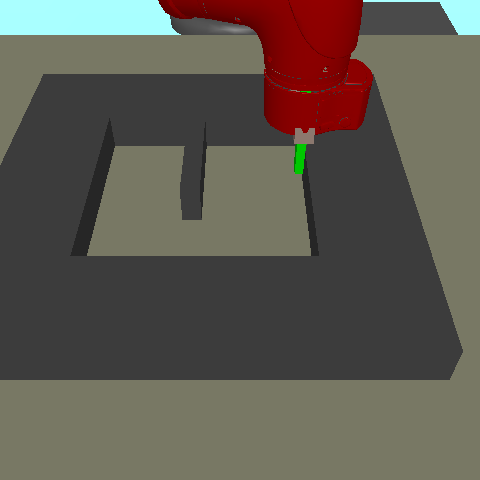
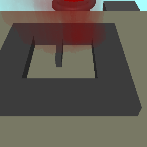
The BackgroundSubtractorMOG2 learns to classify non-moving objects in a scene as background, and any pixel values that fall outside a variance threshold of the Gaussian Mixture Model are classified as foreground. Illustrations of the learned background model are shown in Supplementary Figure 5. At test time, objects placed in the environment appear as foreground as their pixel values fall outside the threshold. Similarly, the robot also appears as foreground, for the same reason. We address this issue using a robot segmentation network, explained in detail below.
 |
 |
 |
(a) | (b) | (c) |
In order to remove the robot from the scene, we train a robot segmentation network. To generate training labels, we use the trained background subtraction module, described above. Using the same dataset used to train the OpenCV background subtraction module (with no objects in the scene), we run the OpenCV background subtraction module. Points that are classified as foreground belong to the robot. We use this output as “ground-truth” segmentation labels. Using these labels, we train a network to segment the robot from the background. We use U-Net [ronneberger2015u] as the segmentation network. The U-Net model we use has 4 blocks of down-sampling convolutions and then 4 blocks of up-sampling covolutions. Every block has a max-pool layer, two convolutional layers each followed by a batch normalization layer and a ReLU activation. Each up-sampling layer has input channels concatenated from the outputs of its down-sampling counterpart. These additional features concatenated from the input convolutions help propagate context information to the higher resolution up-sampling layers. The kernel size is 3x3, with stride 1 and padding 1 for all the convolutional layers.
We train the network using a binary cross entropy loss. The optimization is performed using Nesterov momentum gradient descent for 30 epochs with a learning rate of 1e-3, momentum of 0.9, and a weight decay of 5e-4.
One potential issue of the above method is that the robot segmentation module has only been trained on images without objects in the scene. We find that adding synthetic distractors to the scene helps to improve performance. In this work, we use distractors created by masks of objects similar to those at test time. In future work, we will instead use diverse distractors taken from the COCO dataset [lin2014microsoft].
Appendix E Simulated task details
 |
 |
 |
 |
 |
(a) | (b) | (c) | (d) | (e) |
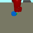
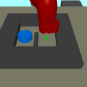
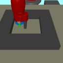
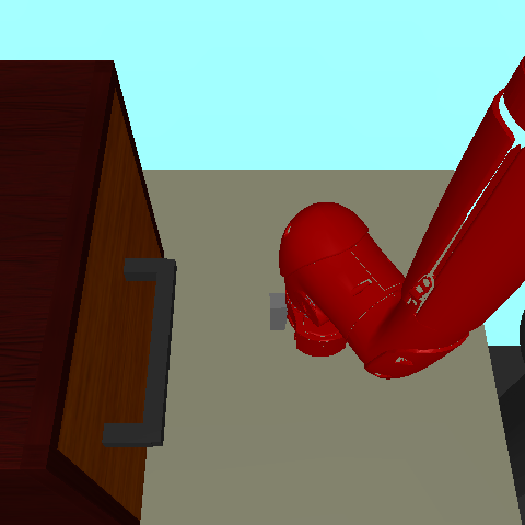
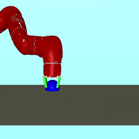
All the tasks are simulated using the MuJoCo [todorov2012mujoco] physics engine. The Puck Pushing, Door Opening, and Object Pickup tasks are identical to those used in Skew-Fit [skewfit]. Illustrations of the environments are shown in Supplementary Figure 6(a), (d), and (e). We also added two additional environments with obstacles and challenging occlusions, shown in Supplementary Figure 6(b) and (c).
For the coordinates used in the puck pushing tasks, the x-axis goes towards the right direction, and the y-axis goes towards the bottom direction in Supplementary Figure 6.
Puck Pushing: A 7-DoF Sawyer arm must push a small puck on a table to various target positions. The agent controls the arm by commanding the movement of the end effector (EE). The underlying state is the EE position and the puck position . The evaluation metric is the distance between the goal and final achieved puck positions. The hand goal/state space is a box . The puck goal/state space is a box . The action space ranges in the interval in the dimensions. The arm is always reset to and the puck is always reset to .
Hurdle-Bottom Puck Pushing: The task is similar to that of Puck Pushing, except we add hurdles on the table to restrict the movement of the puck. The coordinates of the inner corners of the hurdle are top-left , top-right , bottom-left , bottom-right . The left corridor to the middle-hurdle has a width of , and the right corridor to the middle-hurdle has a width of . The corridor up to the hurdle has a width of . The middle-hurdle has a width of and a length of . The arm is always reset to the location of and the puck is reset to . The puck goal space is (i.e., roughly the range of the left corridor). The hand goal space is (i.e., roughly the bottom part of the right corridor).
Hurdle-Top Puck Pushing: The task is similar to that of Hurdle-Bottom Puck Pushing, except the position of the middle-hurdle is flipped. The arm is always reset to and the puck is randomly reset to be in (i.e., roughly the top part of the right corridor). The puck goal space is (i.e., roughly the top part of the left corridor), and the hand goal space is (i.e., roughly the top part of the right corridor).
Door Opening: A 7-DoF Sawyer arm must pull a door on a table to various target angles. The agent control is the same as in Puck Pushing, i.e., the movement of the end effector. The evaluation metric is the distance between the goal and final door angle, measured in radians. In this environment, we do not reset the position of the hand or door at the end of each trajectory. The state/goal space is a cm3 box in the dimension respectively for the arm and an angle between radians for the door. The action space ranges in the interval in the , and dimensions.
Object Pickup: A 7-DoF Sawyer arm must pick up an object on a table to various target positions. The object is cube-shaped, but a larger intangible sphere is overlaid on top so that it is easier for the agent to see. Moreover, the robot is constrained to move in 2 dimension: it only controls the y, z arm positions. The x position of both the arm and the object is fixed. The evaluation metric is the distance between the goal and final object position. For the purpose of evaluation, 75% of the goals have the object in the air and 25% have the object on the ground. The state/goal space for both the object and the arm is 10cm in the y dimension and 13cm in the z dimension. The action space ranges in the interval in the y and z dimensions.
Appendix F Implementation details
Our implementation of ROLL is based on the open-source implementation of Skew-Fit in RLkit111https://github.com/vitchyr/rlkit. For all simulated tasks, the image size is . A summary of the task specific hyper-parameters of ROLL are shown in Supplementary Table 1. The first 4 rows use the same hyper-parameters as in Skew-Fit [skewfit], and the next 5 rows use new hyper-parameters introduced in our work, described in more detail below.
F.1 Network Architectures
We first describe the network architecture of each component in ROLL. For the scene-VAE, we use the same architecture as that in Skew-Fit. In more detail, the VAE encoder has three convolutional layers with kernel sizes: , , and , number of output filters: , , and ; and strides: , , and . The final feature map is mapped by a fully connected layer into a final feature vector of size , and then we have another fully connected layer to output the final latent embedding. The decoder has a fully connected layer that maps the latent embedding into a vector of dimension . This vector is then reshaped into a feature map of size . The decoder has 3 de-convolution layers with kernel sizes , , , number of output filters , , and , and strides , , and .
The object-VAE has almost the same architecture as the scene-VAE. However, the object-VAE has a simpler task that it only needs to encode the segmented object, rather than the entire scene. Thus, for tasks that manipulate a simple object (i.e., all the puck pushing tasks), we use a smaller final feature vector – the final encoder feature vector is of size instead of (details are shown in Supplementary Table 1). Both VAEs have a Gaussian decoder with identity variance; thus the log likelihood loss used to train the decoder is equivalent to a mean-squared error loss.
We use the same latent dimension and for the scene and object-VAE but vary them across different tasks, as shown in Supplementary Table 1. We use the same values of as in Skew-Fit for all tasks. We also use the same latent dimension size for the Door Opening task and the Object Pickup task, and increase the latent dimension size from 4 to 6 for the puck pushing task compared to the original Skew-Fit implementation.
The input to the LSTM is the latent vector from the object-VAE. The LSTM for all tasks has 2 layers and a hidden size of 128 units.
For the policy and Q-network used in SAC, we use exactly the same architecture as in Skew-Fit. For both networks, we use fully connected networks with two hidden layers of size 400 and 300 each, and use ReLU as the activation function.
| Hyper-parameter |
|
|
|
|
|
||||||||||
| Trajectory Length | |||||||||||||||
| for VAE | |||||||||||||||
| Latent Dimension Size | |||||||||||||||
| Skew-Fit for scene-VAE | |||||||||||||||
| object-VAE batch size | 64 | 64 | 128 | 64 | 64 | ||||||||||
| VAE matching loss coefficient | |||||||||||||||
| LSTM matching loss coefficient | |||||||||||||||
| LSTM training schedule (see text) | C | B | B | B | A | ||||||||||
|
6 | 6 | 6 | 576 | 576 |
F.2 Training schedules
We train the scene-VAE using the regular -VAE loss, i.e., the image reconstruction loss and the KL regularization loss. We pre-train it using images obtained by running a random policy for epochs. In each epoch we train for 25 batches with a batch size of 64 and a learning rate of . We also continue to train the scene-VAE alongside during RL training, using images stored in the replay buffer. We sample images from the replay buffer using a skewed distribution as implemented in Skew-Fit. For different tasks we use different skewness as shown in Supplementary Table 1, which is the same as in Skew-Fit. For online training of the scene-VAE, Skew-Fit use three different training schedules for different tasks, and we follow the same training schedule as in Skew-Fit. For details on the training schedule, please refer to appendix C.5 of the Skew-Fit paper.
We train the object-VAE using the image reconstruction loss, the KL regularization loss, and the matching loss. For different tasks we use different coefficients for the matching loss, as shown in Supplementary Table 1. We pre-train the object-VAE with 2000 segmented images obtained by randomly putting the object in the scene. The object-VAE is trained for 2000 epochs, where in each epoch we train for 25 batches with a batch size of 64, except for Hurdle-Top Puck Pushing in which we use a batch size of 128. We use a learning rate of . After the pre-training, the object-VAE is fixed during RL learning. For the synthetic occlusions we add for computing the matching loss, we randomly drop 50% pixels in the segmented objects.
We train the LSTM using an auto-encoder loss and matching loss. For different tasks, we use different coefficients for the matching loss, as shown in Supplementary Table 1. We pre-train the LSTM on the same dataset we use to pre-train the object-VAE, using the auto-encoder loss for 2000 epochs. In each epoch we train for 25 batches with a batch size of 64 and a learning rate of . We continue training the LSTM during the RL learning process. During online training, the training trajectories are sampled uniformly from the SAC replay buffer, and we use both the matching loss and the auto-encoder loss to train the LSTM. We use a learning rate of for training the LSTM. For different tasks we use a different online training schedule for the LSTM, which can be viewed as a counterpart for the online VAE training schedule proposed in Skew-Fit, but with smaller batch sizes, as we use batches of trajectories for training the LSTM. They are detailed as below:
-
1.
Schedule A: For first 5K steps: Train LSTM every 500 time steps for 80 batches, each batch with 25 trajectories. For 5k - 150k steps, train the LSTM every 500 time steps for 20 batches. After 150k steps, train the LSTM every 1500 time steps for 20 batches.
-
2.
Schedule B: For first 5K steps: Train LSTM every 500 time steps for 80 batches, each batch with 25 trajectories. For 5k - 50k steps, train the LSTM every 500 time steps for 20 batches. After 50k steps, train the LSTM every 1000 time steps for 20 batches.
-
3.
Schedule C: For first 5K steps: Train LSTM every 500 time steps for 80 batches, each batch with 25 trajectories. For 5k - 50k steps, train the LSTM every 500 time steps for 20 batches. For 50k - 200k steps, train the LSTM every 1000 time steps for 20 batches. After 200k steps, we stop training the LSTM.
For the SAC training schedule, we use the default values as in Skew-Fit; these values are summarized in Supplementary Table 2.
| Hyper-parameter | Value |
| # training batches per time step | |
| RL Batch Size | |
| Discount Factor | |
| Reward Scaling | |
| Replay Buffer Size | |
| Soft Target | |
| Target Update Period | |
| Use Automatic tuning | True |
| Policy Learning Rate | |
| Q-function Learning Rate |