A theoretical scenario for Galactic RR Lyrae in the Gaia database: constraints on the parallax offset

Abstract

On the basis of an extended set of nonlinear convective RR Lyrae pulsation models we derive the first theoretical light curves in the Gaia bands $G$, $G_{BP}$ and $G_{RP}$ and the corresponding intensity-weighted mean magnitudes and pulsation amplitudes. The effects of chemical composition on the derived Bailey diagrams in the Gaia filters are discussed for both Fundamental and First Overtone mode pulsators. The inferred mean magnitudes and colors are used to derive the first theoretical Period-Wesenheit relations for RR Lyrae in the Gaia filters. The application of the theoretical Period-Wesenheit relations for both the Fundamental and First Overtone mode to Galactic RR Lyrae in the Gaia Data Release 2 database and complementary information on individual metal abundances, allows us to derive theoretical estimates of their individual parallaxes. These results are compared with the astrometric solutions to conclude that a very small offset, consistent with zero, is required in order to reconcile the predicted distances with Gaia results.

1 Introduction

RR Lyrae are old low mass stars that, during the central Helium burning phase, show mainly radial pulsation while crossing the classical instability strip in the Color-Magnitude diagram. From the observational point of view, they represent the most numerous class of pulsating stars in the Milky Way and, being associated to old stellar populations, are typically found in globular cluster and abundant in the Galactic halo and bulge. The investigation of RR Lyrae properties is motivated by their important role both as distance indicators and tracers of old stellar populations. In particular, evolving through the central Helium burning phase, they represent the low mass, Population II counterparts of Classical Cepheids, as powerful standard candles and calibrators of secondary distance indicators. In particular, they can be safely adopted to infer distances to Galactic globular clusters (see e.g. Coppola et al., 2011; Braga et al., 2016, 2018, and references therein), the Galactic center (see e.g. Contreras Ramos et al., 2018; Marconi & Minniti, 2018; Griv et al., 2019) and Milky Way satellite galaxies (see e.g. Coppola et al., 2015; Martínez-Vázquez et al., 2019; Vivas et al., 2019, and references therein). Being associated to old stellar populations, they represent the basis of an alternative Population II distance scale (see e.g. Beaton et al., 2016, to the traditionally adopted Classical Cepheids), more suitable to calibrate secondary distance indicators that are not specifically associated to spiral galaxies (e.g. the Globular Cluster Luminosity Function, see Di Criscienzo et al., 2006, and references therein). The properties that make RR Lyrae standard candles are: i) the well known relation connecting the absolute visual magnitude $M_{V}$ to the metal abundance ${\rm[Fe/H]}$ (see e.g. Sandage, 1993; Caputo et al., 2000; Cacciari & Clementini, 2003; Catelan et al., 2004; Di Criscienzo, Marconi & Caputo, 2004; Federici et al., 2012; Marconi, 2012; Marconi et al., 2015, 2018; Muraveva et al., 2018, and references therein); ii) the Period-Luminosity relation in the Near-Infrared (NIR) filters and in particular in the K 2.2 $\mu{m}$ band (see e.g. Longmore et al., 1990; Bono et al., 2003; Dall’Ora et al., 2006; Coppola et al., 2011; Ripepi et al., 2012; Coppola et al., 2015; Marconi et al., 2015; Muraveva et al., 2015; Braga et al., 2018; Marconi et al., 2018, and references therein). In spite of the well-known advantage of using NIR filters (see e.g. Marconi, 2012; Coppola et al., 2015, and references therein), in the last decades there has been a debate on the coefficient of the metallicity term of the K Band PL relation (see e.g. Bono et al., 2003; Sollima et al., 2006; Marconi et al., 2015, and references therein). On the other hand, it is interesting to note that many recent determinations (see e.g. Sesar et al., 2017; Muraveva et al., 2018) seem to converge towards the predicted coefficient by Marconi et al. (2015), with values in the range 0.16-0.18 mag/dex. As for the optical bands, our recently developed theoretical scenario (Marconi et al., 2015) showed that, apart from the $M_{V}-{\rm[Fe/H]}$ relation that is affected by a number of uncertainties (e.g. a possible nonlinearity, the metallicity scale with the associated $\alpha$ elements enhancement and helium abundance variations, as well as evolutionary effects, see Caputo et al., 2000; Marconi et al., 2018, for a discussion), the metal-dependent Period-Wesenheit (PW) relations are predicted to be sound tools to infer individual distances. In particular, for the B,V band combination, Marconi et al. (2015) demonstrated that the inferred PW relation is independent of metallicity. In order to test this theoretical tool, we need to compare the predicted individual distances with independent reliable distance estimates, as for example the astrometric ones recently obtained by the Gaia satellite (Gaia Collaboration et al., 2016). To this purpose, in the present paper we transform the predicted light curves derived for RR Lyrae models with a wide range of chemical compositions (Marconi et al., 2015, 2018) into the Gaia bands, derive the first theoretical PW relations in these filters and apply them to Gaia Data Release 2 Database (hereinafter Gaia DR2 Gaia Collaboration et al., 2018; Clementini et al., 2019; Ripepi et al., 2019). The organization of the paper is detailed in the following. In Section 2 we summarize the adopted theoretical scenario, while in Section 3 we present the first theoretical light curves in the Gaia filters. From the inferred mean magnitudes and colors the new theoretical PW relations are derived in Section 4, that also includes a discussion of the effects of variations in the input chemical abundances. In Section 5 the obtained relations are applied to Gaia Galactic RR Lyrae with available periods, parallaxes and mean magnitudes to infer independent predictions on their individual parallaxes, to be compared with Gaia DR2 results. The conclusions close the paper.

2 The theoretical scenario

In two recent papers (Marconi et al., 2015, 2018), we presented an updated theoretical scenario for RR Lyrae stars. In Marconi et al. (2015) a wide range of chemical abundances was considered, spanning from typical metal-poor globular clusters values ($Z=0.0001$) to typical abundances of Galactic Disk and Bulge RR Lyrae ($Z=0.02$), with a standard helium content ranging from $Y=0.245$ for the most metal poor abundances to $Y=0.28$ at solar metallicity (see Marconi et al., 2015, for details). Moreover, two stellar masses and three luminosity levels were adopted for each selected chemical composition, in order to take into account not only RR Lyrae located on the Zero Age Horizontal Branch (ZAHB) but also evolved objects (see Marconi et al., 2015, for details). In order to take into account possible variations in the helium abundance, in Marconi et al. (2018) we recomputed the model sets presented in Marconi et al. (2015) by increasing the helium content to $Y=0.30$ and $Y=0.40$ (see Marconi et al., 2018; Marconi & Minniti, 2018, for details). For each selected combination of $Z$, $Y$, stellar mass and luminosity, the system of nonlinear hydrodinamical and convective equations was integrated till a stable limit cycle is achieved in the Fundamental (F) or First Overtone (FO) mode. The resulting bolometric light and radial velocity curves represent an extended dataset of theoretical templates allowing the investigation of the effect of both $Z$ and $Y$ not only on the pulsation period but also on the amplitude and the morphology of the luminosity and radial velocity variations. A similar analysis can be performed with radius curves and the variations of all other relevant quantities, e.g. gravity and temperature, along a pulsation cycle. A subset of the produced theoretical atlas, for $Z=0.001$, $Y=0.245$, $M=0.64M_{\odot}$ and $\log{L=1.67}$, is shown in Figures 1 and 2 for F and FO models, respectively. In each left panel the bolometric light curve is plotted for the labelled effective temperature, whereas the corresponding radial velocity is shown in the right panel, with the labelled period value.

Figure 1: Predicted bolometric light curves for F-mode RR Lyrae models assuming $Z=0.001$, $Y=0.245$, $M=0.64M_{\odot}$ and $\log{L=1.67}$. In each left panel the bolometric light curve is plotted for the labelled effective temperature, whereas the radial velocity curve is shown in the corresponding right panel, with the labelled period value.

Figure 2: The same as Figure 1 but for FO-mode RR Lyrae models at the same chemical composition, mass and luminosity.

These plots show an example of theoretical bolometric magnitude and radial velocity variations that are made available to the community upon request as based on the models computed in Marconi et al. (2015, 2018)

3 Theoretical light curves for RR Lyrae in the Gaia filters

The predicted bolometric light curves discussed above have been transformed into the Gaia bands, namely $G$, $G_{BP}$ and $G_{RP}$, by using the Bolometric Corrections (BC) tables provided by Chen, et al. (2019). This database is based on the most recent and adopted spectral libraries and covers a wide variety of photometric systems, including the Gaia passbands (see Chen, et al., 2019, for all the details). Moreover, these authors provide BC tables for different elemental composition values covering the range considered in this work. By adopting the effective temperature $T_{e}$ and the gravity $\log(g)$ model curves as input, we used a proprietary C code to interpolate the BC tables. When the chemical composition of our models coincides with one specific value of Chen, et al. (2019) grid, we select one BC table and a bi-linear interpolation is performed along the $T_{e}-\log(g)$ direction. On the other hand, if the chemical composition of our models falls between two of the quoted BC tables, we first apply our routine on each neighbouring table, and then interpolate linearly between the two metallicity values. For this procedure we used $M_{bol}^{\odot}=4.79$ mag, consistently with the value adopted in the pulsation code. If the most recent IAU accepted value of the sun bolometric magnitude (4.74 mag) were assumed instead of the adopted 4.79 mag, we would obtain differences in the predicted individual mean magnitudes of the order of 0.01-0.02 mag. In Figures from 3 to 9 we show the first theoretical RR Lyrae light curves transformed into the Gaia bands changing the metallicity (from $Z=0.0001$ to $Z=0.02$, see captions) and considering both F (top panels) and FO (bottom panels) models. The stellar parameter selection is the same as in Marconi et al. (2015).

Figure 3: Theoretical light curves transformed into the Gaia filters $G_{BP}$ (orange), $G$ (green) and $G_{RP}$ (blue) for F-mode (top) and FO-mode (bottom) RR Lyrae models assuming $Z=0.0001$, $Y=0.245$ and $M=0.80M_{\odot}$.

Figure 4: The same as in Figure 3 but assuming $Z=0.0003$, $Y=0.245$ and $M=0.716M_{\odot}$.

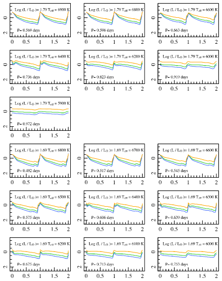
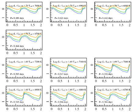
Figure 5: The same as in Figure 3 but assuming $Z=0.0006$, $Y=0.245$ and $M=0.67M_{\odot}$.

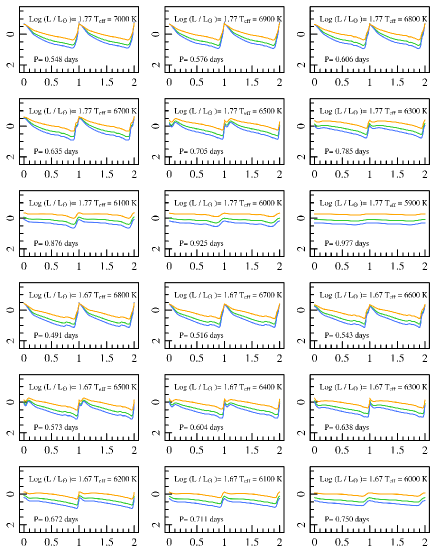
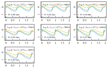
Figure 6: The same as in Figure 3 but assuming $Z=0.001$, $Y=0.245$ and $M=0.64M_{\odot}$.

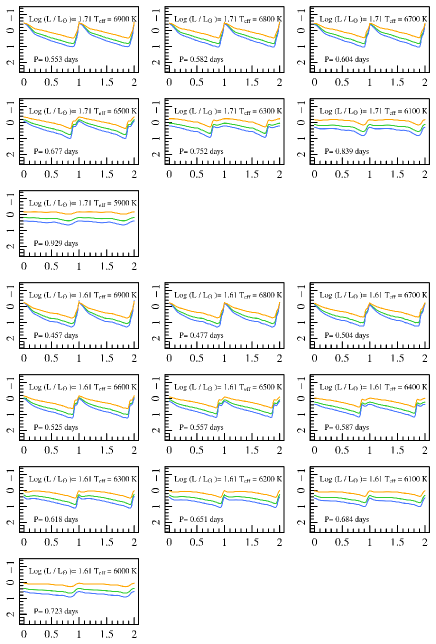
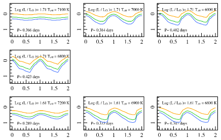
Figure 7: The same as in Figure 3 but assuming $Z=0.004$, $Y=0.25$ and $M=0.59M_{\odot}$.

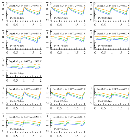
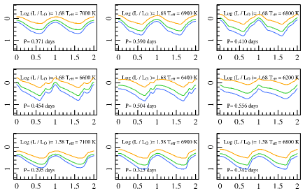
Figure 8: The same as in Figure 3 but assuming $Z=0.008$, $Y=0.256$ and $M=0.57M_{\odot}$.

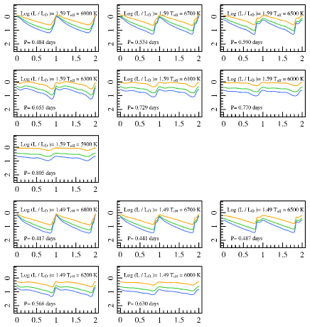
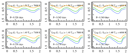
Figure 9: The same as in Figure 3 but assuming $Z=0.02$, $Y=0.27$ and $M=0.54M_{\odot}$.

Similar plots but varying the helium abundance, up to 0.30 and 0.40, for the stellar masses and luminosities as in Marconi et al. (2018) are available upon request to the authors. These plots show that the amplitude and morphology of the light curves in the Gaia bands follow the same trends with the effective temperature as in the optical bands (see e.g. Marconi et al., 2015, and references therein). In particular, we notice that:

1. At fixed mass and luminosity, the pulsation amplitude of F light curves generally decrease as the effective temperature decreases and the pulsation period increases (see also Section 4 for more details).

2. First overtone amplitudes do not show a linear behaviour with the pulsation period, as they reach a maximum towards the center of the FO instability strip to decraese again towards the red edge (bell shape, see Bono et al., 1997, for details).

3. The morphology of F light curves is much more complicated than for FO models, with the presence of bumps and dips related to the coupling between pulsation and convection in the pulsating envelope (see e.g. discussion in Bono & Stellingwerf, 1994; Bono et al., 1997; Di Criscienzo, Marconi & Caputo, 2004).

The data points for the plotted theoretical $G$, $G_{BP}$ and $G_{RP}$ light curves are again available upon request. These are used to infer mean magnitudes and colors as well as pulsation amplitudes, as discussed in the following.

3.1 The Bailey Diagram

On the basis of the transformed light curves discussed above, we are able to build the first predicted Bailey diagram in the three Gaia bands, varying both $Z$ and $Y$. In Figure 10 we show the $G_{BP}$ (top panel), $G$ (middle panel) and $G_{RP}$ (lower panel) pulsation amplitudes as a function of the pulsation period for the labelled metallicities, the corresponding predicted ZAHB masses (see Marconi et al., 2015, for details), namely 0.80$M_{\odot}$ for Z=0.0001, 0.64$M_{\odot}$ for Z=0.001 and 0.57$M_{\odot}$ for Z=0.008, standard $Y$ as in Marconi et al. (2015) and two luminosity levels corresponding to the ZAHB level (solid lines) and a brighter luminosity by 0.1 dex (evolved stage, dotted lines), for each fixed mass. We notice that, in agreement with previous empirical and theoretical results in the optical and near-infrared filters, the following trends can be seen:

• the pulsation amplitudes decrease as the band central wavelength and the metallicity increase;

• an increase in the luminosity level produces a period shift towards longer values. On this basis, in the case of FO RR Lyrae, the location of the described bell-shape in the Bailey diagram can be used to constrain the luminosity level (see e.g. Bono et al., 1997).

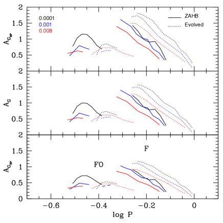
Figure 10: The Bailey diagram in the $G_{BP}$ (top panel), $G$ (middle panel) and $G_{RP}$ (lower panel) filters for the labelled metal abundances, the corresponding predicted ZAHB masses (see Marconi et al., 2015, for details), namely 0.80$M_{\odot}$ for Z=0.0001, 0.64$M_{\odot}$ for Z=0.001 and 0.57$M_{\odot}$ for Z=0.008, standard $Y$ as in Marconi et al. (2015) and two luminosity levels corresponding to the ZAHB level (solid line) and a brighter luminosity by 0.1 dex (dotted line), for each fixed mass.

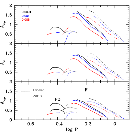
Figure 11: The Bailey diagram in the $G_{BP}$ (top panel), $G$ (middle panel) and $G_{RP}$ (lower panel) filters for the labelled metal abundances and Y=0.30, the corresponding predicted ZAHB masses (see Marconi et al., 2015, for details), namely 0.80$M_{\odot}$ for Z=0.0001, 0.64$M_{\odot}$ for Z=0.001 and 0.56$M_{\odot}$ for Z=0.008, and two luminosity levels corresponding to the ZAHB level (solid line) and a brighter luminosity by 0.1 dex (dotted line), for each fixed mass.

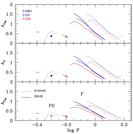
Figure 12: The Bailey diagram in the $G_{BP}$ (top panel), $G$ (middle panel) and $G_{RP}$ (lower panel) filters for the labelled metal abundances and Y=0.40, the corresponding predicted ZAHB masses (see Marconi et al., 2015, for details), namely 0.69$M_{\odot}$ for Z=0.0001, 0.62$M_{\odot}$ for Z=0.001 and 0.55$M_{\odot}$ for Z=0.008, and two luminosity levels corresponding to the ZAHB level (solid line) and a brighter luminosity by 0.1 dex (dotted line), for each fixed mass. In the case of FO models with $Z=0.0001$ and $Y=0.40$ we find only one case for each of the two luminosity levels, that are indicated as filled (ZAHB) and open (evolved) circles.

By including the He-enriched pulsation models computed in Marconi et al. (2018) we can investigate the effect of a possible helium enrichment. In Figures 11 and 12 we reproduce the Gaia filters Bailey diagram but assuming $Y=0.30$ and $Y=0.40$, respectively. By comparing these plots with the standard helium case (Figure 9) we notice that, as the helium abundance increases, two main trends occur:

1. The periods get systematically longer as an effect of the increased ZAHB luminosity level (see e.g. Marconi et al., 2018; Marconi & Minniti, 2018, and references therein)

2. The pulsation amplitudes get systematically smaller, mainly as an effect of the reduced hydrogen abundance.

3.2 Mean magnitudes and colors

From the theoretical RR Lyrae Gaia filter light curves we can derive intensity weighted mean magnitudes. These are reported, for each individual model, in Tables 1 and 2, for the F and FO-mode, respectively. The various columns in these tables report the metal and helium abundances, the predicted pulsation period, the input mass, luminosity (in solar units), effective temperature and the inferred mean magnitudes and pulsation amplitude in the three filters $G_{BP}$, $G$ and $G_{RP}$. On this basis the color index $<G_{BP}>-<G_{RP}>$ can also be derived, for each pulsation model, and the theoretical PW relations can be computed for each individual chemical composition or directly including a metallicity and a helium abundance term, as discussed in the following Section.

4 The theoretical Period-Wesenheit relations

From the intensity-weighted mean magnitudes reported in Tables 1 and 2, we can derive the first theoretical PW relations in the Gaia filters for RR Lyrae stars, as a function of the metal abundance. The definition of the adopted Wesenheit relation is the same as in De Somma et al. (2020), namely $G-1.9(<G_{BP}>-<G_{RP}>)$, that in turn was based on the derivation by Ripepi et al. (2019). Additional relations, including Helium enriched models, and thus providing the dependence on $Y$ as well, are also derived. The coefficients of the PW relations including only the metallicity term or both the metallicity and the helium abundance, are reported in Tables 3 and 4, respectively. These relations are derived both separately for the two pulsation modes (first two lines of Tables 3 and 4) and globally, by fundamentalizing FO periods (see Marconi et al., 2015; Coppola et al., 2015, and references therein) according to the relation $\log{P_{F}}=\log{P_{FO}}+0.127$ (last line of Tables 3 and 4).

Table 1: Fundamental model parameters: $Z$ and $Y$ values are listed in columns 1 and 2, respectively, the pulsational period of the model is in column 3, the mass, luminosity and effective temperatures are listed in columns 4,5 and 6, while the Gaia light curve intensity average magnitudes and amplitudes are reported in columns 7, 8, for the $BP$ band, 9, 10 for the $G$ band and 11, 12 for the $RP$ band. The complete table is available in electronic format.

$Z$	$Y$	$P$	$M$	$\log(L/L_{\odot})$	$T_{e}$	$<BP>$	$Amp(BP)$	$<G>$	$Amp(G)$	$<RP>$	$Amp(RP)$
		$(days)$	$(M_{\odot})$	$(dex)$	$(K)$	$(mag)$	$(mag)$	$(mag)$	$(mag)$	$(mag)$	$(mag)$
0.0001	0.245	0.9800	0.80	1.860	5900	0.173	0.260	-0.056	0.219	-0.442	0.163
0.0001	0.245	0.9261	0.80	1.860	6000	0.162	0.527	-0.059	0.452	-0.434	0.343
0.0001	0.245	0.8776	0.80	1.860	6100	0.149	0.656	-0.062	0.566	-0.424	0.430
0.0001	0.245	0.8292	0.80	1.860	6200	0.136	0.936	-0.065	0.811	-0.413	0.611
0.0001	0.245	0.7444	0.80	1.860	6400	0.108	1.157	-0.070	1.014	-0.383	0.783
0.0001	0.245	0.6692	0.80	1.860	6600	0.092	1.577	-0.062	1.373	-0.338	1.017
						…

Table 2: First overtone model parameters: $Z$ and $Y$ values are listed in columns 1 and 2, respectively, the pulsational period of the model is in column 3, the mass, luminosity and effective temperatures are listed in columns 4,5 and 6, while the Gaia light curve intensity average magnitudes and amplitudes are reported in columns 7, 8, for the $BP$ band, 9, 10 for the $G$ band and 11, 12 for the $RP$ band. The complete table is available in electronic format.

$Z$	$Y$	$P$	$M$	$\log(L/L_{\odot})$	$T_{e}$	$<BP>$	$Amp(BP)$	$<G>$	$Amp(G)$	$<RP>$	$Amp(RP)$
		$(days)$	$(M_{\odot})$	$(dex)$	$(K)$	$(mag)$	$(mag)$	$(mag)$	$(mag)$	$(mag)$	$(mag)$
0.0001	0.245	0.4720	0.80	1.860	6700	0.072	0.723	-0.078	0.630	-0.346	0.476
0.0001	0.245	0.4496	0.80	1.860	6800	0.061	0.784	-0.078	0.681	-0.329	0.507
0.0001	0.245	0.4274	0.80	1.860	6900	0.052	0.853	-0.077	0.736	-0.312	0.531
0.0001	0.245	0.4082	0.80	1.860	7000	0.044	0.808	-0.076	0.697	-0.295	0.499
0.0001	0.245	0.3897	0.80	1.860	7100	0.034	0.499	-0.079	0.431	-0.284	0.309
0.0001	0.245	0.4107	0.80	1.760	6600	0.339	0.686	0.178	0.594	-0.109	0.441
						…

Table 3: The coefficients of the metal-dependent PW relations $W=a+b\log{P}+c{\rm[Fe/H]}$ for F and FO models. The last column represents the root-mean-square-deviation ($\sigma$) coefficient

mode	a	b	c	$\sigma_{a}$	$\sigma_{b}$	$\sigma_{c}$	$\sigma$
F	-0.936	-2.296	0.124	0.049	0.032	0.005	0.05
FO	-1.344	-2.440	0.112	0.033	0.028	0.005	0.03
GLOBAL	-0.952	-2.271	0.123	0.051	0.024	0.004	0.05

Table 4: The coefficients of the metal- and helium-dependent PW relations $W=a+b\log{P}+c{\rm[Fe/H]}+d\log{Y}$ for F and FO models

. The last column represents the root-mean-square-deviation ($\sigma$) coefficient. mode a b c d $\sigma_{a}$ $\sigma_{b}$ $\sigma_{c}$ $\sigma_{d}$ $\sigma$ F -1.277 -2.298 0.123 -0.573 0.044 0.014 0.003 0.028 0.04 FO -1.600 -2.436 0.120 -0.442 0.031 0.020 0.003 0.031 0.03 GLOBAL -1.278 -2.257 0.126 -0.558 0.047 0.012 0.002 0.025 0.05

In Figure 13 we plot the predicted Gaia band Wesenheit relations, varying the metallicity from $Z=0.0001$ to $Z=0.02$, at standard helium content, for F and FO models (upper panel) and combining F with fundamentalized FO models in a global relation (bottom panel).

Figure 13: The theoretical PW relations in the Gaia filters, varying the metal abundance from $Z=0.0001$ to $Z=0.02$ (more metallic relations are fainter, see the labelled arrow) and standard Y (as in Marconi et al., 2015), for F and FO models (upper panel) and combining F with fundamentalized FO models in a global relation (bottom panel).

We notice that a metallicity variation can change the zero point of the relation by a few tenths of magnitude. In particular, the zero point gets fainter as the metallicity increases (see labelled arrow).

The effect of a variation in the helium content is shown in Figure 14. Here the same relations presented in Figure 13 are compared with their counterparts for $Y=0.30$ (red lines) and $Y=0.40$ (blue lines), respectively, for the F (top panel) and FO (middle panel) mode, as well as for the global selection (bottom panel). According to these plots $Y$ seems to have a minor effect on the slope and the zero point of PW relations even if the period range gets systematically longer and the Wesenheit functions systematically brighter as the helium content increases. These trends are due to the effects of the increased ZAHB luminosity level on the pulsation periods and mean magnitudes as the helium content increases (see Marconi et al., 2018, for details).

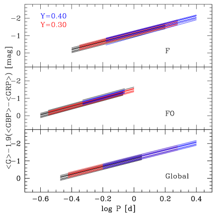
Figure 14: The theoretical PW relations in the Gaia filters, varying the Helium abundance from the standard value (as in Fig. 13, black lines) to $Y=0.30$ (red lines) and $Y=0.40$ (blue lines) for the F (top panel) and FO (middle panel) mode, as well as for the global selection (bottom panel).

5 Predicted parallaxes for Gaia RR Lyrae targets

5.1 Selection of the sample

To test our new predictions we searched the literature for RR Lyrae with both a metallicity estimate and Gaia DR2 photometry in the $G,G_{BP},G_{RP}$ bands calculated as intensity-averaged magnitudes (see Holl et al., 2018; Clementini et al., 2019, for details). More in detail, we scanned the literature searching for RR Lyrae whose metallicity was estimated on the basis of high-resolution spectroscopy (HRS), in order to guarantee accuracy and precision in the measurement. To this aim we first adopted the compilation by Magurno et al. (2018), who listed the HRS iron abundances present in the literature for a sample of 134 RR Lyrae stars. An inspection of their Table 10 showed that several objects were observed two or more times by different Authors. In these cases we averaged the results and took the standard deviation as a measure of the uncertainty. As no error is available for the stars with one single measurement, we considered the errors derived above for the pulsators with at least three independent measurements and calculated the mean, obtaining an average error of 0.13 dex. We therefore assigned this value as minimum uncertainty for stars with single measurements, and, to be conservative, extended this uncertainty also to stars with only two measurements whose semi-difference was smaller than 0.13 dex. The results of this exercise is reported in Table 5, where we listed the 98 stars in Magurno et al. (2018) sample with Gaia DR2 intensity-averaged magnitudes. For completeness, we also reported the stars without $G_{BP},G_{RP}$ magnitudes.

The sample by Magurno et al. (2018) was complemented by searching serendipitous RR Lyrae metallicity measurements among recently published spectroscopic surveys based on HRS, namely APOGEE2-DR16 (Apache Point Observatory Galactic Evolution Experiment 2, Data Release 16 Ahumada et al., 2020) and GALAH Data Release 2 (GALactic Archaeology with HERMES, DR2 Buder et al., 2018). As a result of this search, we found 8 and 61 objects in APOGEE and GALAH, respectively. As APOGEE observes in the near infrared and has a lower resolution, we searched for possible systematic differences in iron abundance with respect to GALAH. To this aim we cross-correlated the entire catalogues of APOGEE and GALAH, using the resulting 515 stars in common, covering an interval $-$0.5$<$[Fe/H]$<$0.5 dex, and calculated the following equation to apply a small correction to APOGEE results: ${\rm[Fe/H]}_{G}=(-0.0155\pm 0.0044)+(1.047\pm 0.016){\rm[Fe/H]}_{A}$, with rms=0.058 dex, where ${\rm[Fe/H]}_{G}$ and ${\rm[Fe/H]}_{A}$ are the iron abundances in the GALAH and APOGEE system, respectively. The iron abundance data with the relative uncertainties for the APOGEE and GALAH survey are shown in Table 5. Note that for the APOGEE data, the table lists the corrected [Fe/H] values and the original uncertainties have been summed in quadrature with the rms error of the relation converting APOGEE into GALAH iron abundanced. The total HRS sample in this table amounts to 167 objects. We applied a further selection to this sample removing all the objects with negative parallax and with RUWE$\geq$1.4 as suggested by the Gaia documentation. Moreover we selected only RR Lyrae with relative parallax error lower than 10$\%$. Therefore the final HRS sample comprises 103 objects.

In addition to the above described sample, upon Referee suggestion, we also adopted the sample by Muraveva et al. (2018), largely based on the work by Dambis et al. (2013), that collected literature metallicities for RR Lyrae derived with different techniques from spectroscopic data at distinct resolutions. Applying the same cuts quoted above, the Muraveva et al. (2018) sample shrinks to 112 objects.

Before proceeding, it is worth comparing the HRS and Muraveva et al. (2018) samples. There are 70 stars in common between these samples. The correlation between the iron abundances is shown in Fig. 15. It can be easily seen that there is a detectable trend with metallicity between the two samples. The linear correlation between the iron content values in the two samples is: ${\rm[Fe/H]}_{HRS}=(0.328\pm 0.092)+(1.265\pm 0.069){\rm[Fe/H]}_{Mur}$, with rms=0.21 dex, where ${\rm[Fe/H]}_{HRS}$ and ${\rm[Fe/H]}_{Mur}$ are the iron abundances in the HRS and Muraveva et al. (2018) samples, respectively.

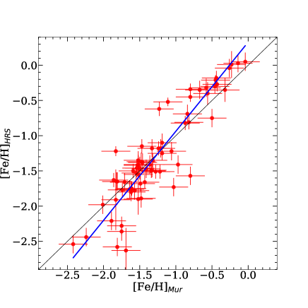
Figure 15: Comparison between the HRS and Muraveva et al. (2018) samples. The 45°is shown a thin black line. The linear regression is displayed as a thick blue line.

5.2 Application of theoretical PWZ relations

In this section we apply to the selected HRS and Muraveva et al. (2018) samples the theoretical PWZ relations reported in Table 3 for the F, FO and global case. The application of the quoted PWZ relations allows us to derive individual distance moduli and, in turn, individual parallaxes to be compared with Gaia DR2 determinations. The differences between the theoretical parallaxes and Gaia DR2 results are shown in Figures 16 and 17, for the HRS and Muraveva et al. (2018) samples, respectively, when applying the F (upper panel), FO (middle panel) and global (bottom panel) PWZ relations. In both figures, blue and red symbols correspond to accepted and discarded objects by a 2.5 $\sigma-$clipping procedure. The error bars take into account the observational parallax error and the intrinsic dispersion of the adopted PWZ relations. The labelled mean weighted differences suggest a very good agreement between theoretical and empirical distance determinations. These results are consistent with the zero-point offset obtained for RR Lyrae by Arenou et al. (2018), who validated Gaia DR2 catalogue finding a negligible ($-$0.01$\pm$0.02 mas) offset between the HST and DR2 parallaxes, and slightly smaller than the offset obtained by Muraveva et al. (2018) (-0.057 mas) for RR Lyrae, by Riess et al. (2018) ($-0.046\pm$0.013 mas) and Ripepi et al. (2019) ($-0.07$ mas) for Classical Cepheids. and by De Somma et al. (2020) from the application of theoretical PW relations at solar chemical composition to a sample of Gaia DR2 Galactic Cepheids, even if still consistent within the errors. Indeed, a different zero-point offset might, in principle, be obtained for Cepheids and RR Lyrae as an effect of its possible dependence on magnitude and color but new more accurate parallaxes, as expected from Gaia Data Release 3 and/ subsequent releases, are needed in order to properly fix this quantity.

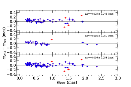
Figure 16: Difference between the theoretical parallaxes and Gaia DR2 results for the F (upper panel), FO (middle panel) and global sample selections, respectively, taking into account the HRS sample discussed in the text. Blue and red symbols correspond to accepted and discarded objects according to a 2.5$\sigma$-clipping procedure.

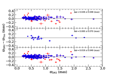
Figure 17: Difference between the theoretical parallaxes and Gaia DR2 results for the F (upper panel), FO (middle panel) and global sample selections, respectively, taking into account the Muraveva et al. (2018) sample discussed in the text. Blue and red symbols correspond to accepted and discarded objects according to a 2.5$\sigma$-clipping procedure.

6 Conclusions

An extensive set of nonlinear convective pulsation models for RR Lyrae at different metal and helium abundances has been taken into account. The transformation of bolometric magnitude variations into the Gaia filters allowed us to derive the first theoretical light curves directly comparable with Gaia time-series data. In particular, we built the first theoretical Bailey diagrams and PW relations in the $G_{BP}$, $G$ and $G_{RP}$ filters, varying both the metallicity and the helium content. As for the Bailey diagram we conclude that an increase in the metal abundance and/or in the helium abundance produces a decrease in the pulsation amplitudes, whereas an increase in the luminosity level produces a period shift towards longer values. In particular, in the case of FO RR Lyrae, the location of the described bell-shape in the Bailey diagram can be used to constrain the luminosity level (see e.g. Bono et al., 1997). The theoretical PW relations in the Gaia bands show a dependence of the zero point on metal abundance, in the sense that brighter Wesenheit functions are predicted for more metal poor chemical composition and a lower effect due to variations in the helium content, with helium enriched models characterized by longer periods and brighter Wesenheit functions. The theoretical PWZ relations are applied to a subset of Gaia DR2 RR Lyrae (293 F and 50 FO pulsators) with complementary metallicity information to infer individual theoretical parallaxes, that are in very good agreement with Gaia results. In particular, the inferred zero-point parallax offset is consistent with zero both in the case of F and FO pulsators. Even if more stringent conclusions could be drawn in the future from the next Gaia data releases, the obtained results seem on one side to support the predictive capabilities of current pulsation models and on the other to suggest that a smaller parallax offset could be required for the bluer older and lower mass RR Lyrae stars than for Classical Cepheids.

7 Data Availability

The multi-band model light curves data are available upon request to the authors. Tables 1 and 2 are published in electronic form.

Appendix A Sample of RR Lyrae with metallicity from high resolution spectroscopy.

Table 5: Sample of RR Lyrae stars used for the comparison with the models with metallicity from high resolution spectroscopy. The meaning of the columns is: (1) Gaia source identifiers; (2) mode of pulsation: RRab, RRc and RRd mean fundamental, first overtone and double mode pulsator, respectively; (3,4) coordinates; (5,6) Gaia parallax and relative error; (7) ruwe parameter (see text); (8) Period; (9,10,11) $G,G_{BP},G_{RP}$ intensity-averaged magnitudes; (12) number of averaged measures: for APOGEE and GALAH survey it was imposed equal to one; (13,14) adopted iron abundance and relative error; (15) source of the iron abundance: APO=APOGEE; GAL=GALAH; M18=Magurno et al. (2018).

ID	Mode	RA	Dec	$\varpi$	$\sigma_{\varpi}$	ruwe	P	G	GBP	GRP	n	[Fe/H]	$\sigma$[Fe/H]	Source
		(J2000)	(J2000)	(mas)	(mas)		days	(mag)	(mag)	(mag)		(dex)	(dex)
(1)	(2)	(3)	(4)	(5)	(6)	(7)	(8)	(9)	(10)	(11)	(12)	(13)	(14)	(15)
ASAS_J184654-5439.3	RRc	281.72510	$-$54.65558	0.3288	0.0348	1.170	0.23413	13.303	13.431	13.038	1	$-$0.46	0.09	GAL
ASAS_J164128-1029.6	RRc	250.36483	$-$10.49337	0.7079	0.0428	1.039	0.23673	12.589	12.951	12.048	1	$-$0.35	0.07	GAL
ASAS_J202817-3806.6	RRc	307.07122	$-$38.11025	0.2621	0.0425	1.219	0.24485	13.261	13.385	13.006	1	$-$0.47	0.07	GAL
KIC8832417	RRc	296.72630	45.08063	0.4842	0.0188	0.936	0.24855	12.998	13.252	12.583	1	$-$0.27	0.13	M18
KIC5520878	RRc	287.59821	40.76791	0.2227	0.0166	1.128	0.26917	14.038	14.222	13.692	1	$-$0.18	0.13	M18
YZCap	RRc	319.88499	$-$15.11706	0.8480	0.0668	1.331	0.27345	11.219	11.384	10.928	2	$-$1.51	0.10	M18
ASAS_J023319-7336.7	RRc	38.32818	$-$73.61193	0.4779	0.0189	1.199	0.28714	11.983	12.116	11.735	1	$-$0.77	0.07	GAL
GDR2_5202509386185816704	RRc	149.90233	$-$78.73859	0.2562	0.0124	1.089	0.29035	13.429	13.631	13.069	1	$-$0.74	0.08	GAL
UCom	RRc	190.01308	27.49887	0.5223	0.0421	1.138	0.29274	11.670	11.537	11.358	1	$-$1.41	0.13	M18
ASASSN_J185318.40-542921.7	RRc	283.32665	$-$54.48947	0.2691	0.0239	1.134	0.29274	13.526	13.678	13.226	1	$-$0.48	0.09	GAL
CRTS_J102704.8-412916	RRc	156.77017	$-$41.48780	0.2655	0.0203	1.144	0.29278	13.576	13.737	13.266	1	$-$0.72	0.08	GAL
ASAS_J110522-2641.0	RRc	166.34138	$-$26.68466	0.5391	0.0371	1.078	0.29446	11.802	11.941	11.551	2	$-$1.69	0.13	M18
CRTS_J201409.3-464306	RRc	303.53934	$-$46.71813	0.2076	0.0325	1.206	0.29982	13.106	13.218	12.854	1	$-$0.58	0.08	GAL
ASAS_J200431-5352.3	RRc	301.13103	$-$53.87190	0.8197	0.0444	1.114	0.30023	11.029	11.166	10.775	2	$-$2.69	0.13	M18
RZCep	RRc	339.80584	64.85932	2.3585	0.0290	0.950	0.30871	9.256	9.556	8.805	1	$-$2.36	0.13	M18
OGLE-SMC-RRLYR-6212	RRc	31.91403	$-$77.81319	0.3228	0.0184	1.159	0.31067	12.581	12.742	12.279	1	$-$0.62	0.08	GAL
ASAS_J203145-2158.7	RRc	307.93716	$-$21.97964	0.7762	0.0428	1.000	0.31071	11.320	11.494	11.025	1	$-$1.17	0.13	M18
CSEri	RRc	39.27456	$-$42.96331	2.0684	0.0279	1.065	0.31133	8.924	9.080	8.676	1	$-$1.89	0.13	M18
TVBoo	RRc	214.15240	42.35977	0.7468	0.0285	1.032	0.31256	10.911	11.041	10.685	1	$-$2.44	0.13	M18
ASAS_J145747-3812.2	RRc	224.44490	$-$38.20380	0.1249	0.1364	1.154	0.31664	13.067	13.301	12.794	1	$-$0.76	0.08	GAL
GDR2_6367478755093421056	RRc	291.66128	$-$74.64357	0.4086	0.0321	1.204	0.31673	12.424	12.612	12.104	1	$-$0.70	0.07	GAL
MTTel	RRc	285.55030	$-$46.65386	1.9331	0.0414	0.927	0.31690	8.911	9.096	8.674	1	$-$2.58	0.13	M18
ASASSN_J190454.75-643958.7	RRc	286.22809	$-$64.66630	0.1288	0.0184	1.097	0.31752	13.937	14.104	13.625	1	$-$0.73	0.09	GAL
TSex	RRc	148.36825	2.05722	1.2466	0.0444	0.996	0.32468	9.964	99.999	99.999	2	$-$1.66	0.10	M18
OGLE-SMC-RRLYR-2621	RRc	357.91003	$-$73.57293	0.3623	0.0211	1.059	0.32635	12.698	12.853	12.409	1	$-$0.87	0.08	GAL
ASAS_J180809-6527.4	RRc	272.03547	$-$65.45624	0.2941	0.0205	1.068	0.32735	13.241	13.424	12.907	1	$-$0.78	0.08	GAL
YCrv	RRc	189.54342	$-$15.00004	0.6695	0.0478	1.208	0.32903	11.554	11.696	11.296	1	$-$1.39	0.13	M18
GDR2_1317846466364172800	RRc	244.85760	29.71312	0.6466	0.0335	1.229	0.33169	11.328	11.469	11.065	1	$-$2.63	0.32	APO
GDR2_6109120799902812928	RRc	207.67380	$-$42.24301	0.4929	0.0295	0.946	0.33264	12.798	13.012	12.462	1	0.33	0.07	GAL
GDR2_1686384274158206208	RRc	195.87937	71.11218	0.9834	0.0343	1.295	0.33298	10.184	10.328	9.888	1	$-$1.62	0.18	APO
KIC4064484	RRc	293.43948	39.12052	0.1688	0.0201	1.102	0.33700	14.421	14.642	14.024	1	$-$1.58	0.13	M18
ASASSN_J211212.83-501250.1	RRc	318.05352	$-$50.21394	0.2539	0.0327	1.167	0.34175	13.806	13.946	13.519	1	$-$0.73	0.08	GAL
AAAql	RRab	309.56279	$-$2.89034	0.6774	0.0506	1.045	0.36177	11.816	11.867	11.467	1	$-$0.32	0.13	M18
KIC9453114	RRc	285.96047	46.02887	0.2132	0.0182	1.322	0.36573	13.285	13.438	12.984	1	$-$2.13	0.13	M18
SVScl	RRc	26.24859	$-$30.05943	0.5014	0.0391	1.108	0.37736	11.304	11.445	11.059	1	$-$2.28	0.13	M18
RSBoo	RRab	218.38841	31.75461	1.3624	0.0396	1.138	0.37737	10.331	10.369	10.078	4	$-$0.35	0.17	M18
GDR2_5779689627114584576	RRc	229.25498	$-$77.93312	0.1762	0.0171	1.074	0.37751	13.812	14.009	13.466	1	$-$0.61	0.09	GAL
AVPeg	RRab	328.01170	22.57479	1.4635	0.0320	1.136	0.39037	10.472	10.692	10.069	3	$-$0.18	0.10	M18
OGLE-SMC-RRLYR-2594	RRc	356.81960	$-$78.70534	0.1629	0.0177	1.122	0.39459	13.910	14.110	13.554	1	$-$0.87	0.09	GAL
V445Oph	RRc	246.17172	$-$6.54162	1.6154	0.0526	1.220	0.39703	10.837	99.999	99.999	5	0.01	0.19	M18
ASAS_J114710-4131.7	RRab	176.79419	$-$41.52862	0.3606	0.0200	1.062	0.39741	13.157	13.409	12.745	1	$-$0.34	0.08	GAL
TWHer	RRab	268.63002	30.41046	0.8596	0.0238	1.151	0.39960	11.208	11.527	10.923	1	$-$0.35	0.13	M18
GDR2_5821920567383108224	RRab	244.04851	$-$65.81513	0.3047	0.0180	1.190	0.40542	13.676	13.936	13.265	1	0.08	0.08	GAL
CNLyr	RRab	280.31643	28.72253	1.1096	0.0262	1.050	0.41138	11.260	11.584	10.784	1	$-$0.04	0.13	M18
WCrt	RRab	171.62345	$-$17.91441	0.7475	0.0449	1.292	0.41201	11.450	11.650	11.138	1	$-$0.75	0.13	M18
ASASSN_J154554.85-401900.1	RRab	236.47853	$-$40.31668	0.2106	0.0332	1.056	0.41335	14.309	14.815	13.779	1	0.29	0.09	GAL
ASAS_J005001-6238.1	RRd	12.50263	$-$62.63541	0.6271	0.0247	1.216	0.41453	12.088	12.383	11.847	1	$-$0.45	0.07	GAL
ASAS_J045314-3749.2	RRab	73.31013	$-$37.82105	0.4704	0.0209	1.228	0.41978	12.043	12.369	11.877	1	$-$0.52	0.06	GAL
DMCyg	RRab	320.29810	32.19129	0.9652	0.0507	1.479	0.41987	11.439	11.783	11.086	1	0.03	0.13	M18
ARPer	RRab	64.32163	47.40014	1.9156	0.0491	1.005	0.42556	10.237	10.615	9.694	3	$-$0.27	0.10	M18
V440Sgr	RRab	293.08657	$-$23.85378	1.3991	0.0408	0.993	0.42893	10.158	10.638	9.922	2	$-$1.15	0.10	M18
GDR2_6362257964645972352	RRab	305.14572	$-$78.30634	0.3064	0.0157	1.201	0.43072	13.449	13.729	12.998	1	$-$0.62	0.09	GAL
V839Cyg	RRab	290.07867	47.13012	0.2171	0.0174	1.065	0.43378	14.454	14.727	14.052	1	$-$0.05	0.13	M18
V1104Cyg	RRab	289.50206	50.75495	0.1024	0.0237	1.216	0.43639	14.635	14.837	14.307	1	$-$1.23	0.13	M18
CRTS_J171304.1+355841	RRab	258.26658	35.97854	0.6270	0.0226	1.058	0.44036	11.380	11.767	11.215	1	$-$1.73	0.13	APO
KXLyr	RRd	278.31341	40.17304	0.9268	0.0239	1.032	0.44091	10.889	11.132	10.598	2	$-$0.30	0.10	M18
CSS_J165135.0-040010	RRab	252.89633	$-$4.00300	0.2429	0.0317	1.081	0.44571	14.279	14.718	13.920	1	$-$0.52	0.09	GAL
VXHer	RRab	247.66978	18.36691	0.9797	0.0589	1.226	0.45536	10.774	99.999	99.999	5	$-$1.42	0.13	M18
RVUMa	RRab	203.32515	53.98720	0.9227	0.0277	1.116	0.46806	10.693	10.891	10.412	2	$-$1.25	0.10	M18

Table 6: continued

ID	Mode	RA	Dec	$\varpi$	$\sigma_{\varpi}$	ruwe	P	G	GBP	GRP	n	[Fe/H]	$\sigma$[Fe/H]	Source
		(J2000)	(J2000)	(mas)	(mas)		days	(mag)	(mag)	(mag)		(dex)	(dex)
(1)	(2)	(3)	(4)	(5)	(6)	(7)	(8)	(9)	(10)	(11)	(12)	(13)	(14)	(15)
V715Cyg	RRab	295.53335	38.91177	0.0732	0.0460	1.055	0.47071	16.401	16.803	15.991	1	$-$1.13	0.13	M18
DXDel	RRab	311.86821	12.46411	1.6849	0.0323	1.049	0.47261	9.808	10.031	9.404	4	$-$0.40	0.16	M18
XZCyg	RRab	293.12277	56.38809	1.5713	0.0273	1.046	0.47360	9.675	99.999	99.999	2	$-$1.55	0.10	M18
V355Lyr	RRab	283.35799	43.15458	0.1911	0.0225	1.280	0.47370	14.289	99.999	99.999	1	$-$1.14	0.13	M18
UUVir	RRab	182.14595	$-$0.45676	1.2086	0.0810	1.125	0.47558	10.516	99.999	99.999	3	$-$0.81	0.10	M18
XZDra	RRab	287.42763	64.85894	1.2956	0.0239	1.064	0.47648	10.163	10.380	9.824	2	$-$0.82	0.10	M18
CRTS_J213829.6-490054	RRd	324.62358	$-$49.01486	0.1764	0.0241	1.221	0.47746	13.649	13.849	13.342	1	$-$0.79	0.08	GAL
CRTS_J134815.9+395403	RRab	207.06647	39.90065	0.5696	0.0228	1.146	0.47852	11.839	12.030	11.512	1	$-$1.90	0.22	APO
ASAS_J202812-4236.2	RRab	307.05117	$-$42.60213	0.1689	0.0278	1.143	0.47938	13.747	13.994	13.464	1	$-$0.83	0.08	GAL
VInd	RRab	317.87415	$-$45.07492	1.4972	0.0410	1.159	0.47959	9.864	10.012	9.562	2	$-$1.46	0.16	M18
V838Cyg	RRab	288.51629	48.19964	0.0642	0.0196	1.320	0.48029	14.051	99.999	99.999	1	$-$1.01	0.13	M18
CRTS_J074506.2+430641	RRab	116.27630	43.11156	0.6227	0.0378	1.093	0.48185	11.863	12.078	11.469	1	$-$0.62	0.10	APO
BRAqr	RRab	354.63709	$-$9.31878	0.6489	0.0491	0.987	0.48188	11.421	99.999	99.999	1	$-$0.69	0.13	M18
V2178Cyg	RRab	295.02901	38.97234	0.1398	0.0293	1.031	0.48702	15.372	15.846	14.976	1	$-$1.66	0.13	M18
OGLE-SMC-RRLYR-5992	RRab	26.84105	$-$73.35031	0.2347	0.0175	1.327	0.48761	13.843	14.091	13.463	1	$-$0.41	0.09	GAL
ASAS_J043355-0025.6	RRab	68.47898	$-$0.42552	0.4097	0.0432	1.140	0.48768	12.627	12.843	12.189	1	$-$0.83	0.12	APO
KIC6100702	RRab	282.65722	41.42380	0.2924	0.0115	1.118	0.48814	13.496	13.719	13.067	1	$-$0.16	0.13	M18
DHHya	RRab	135.06169	$-$9.77900	0.4687	0.0402	1.166	0.48900	12.112	99.999	99.999	1	$-$1.53	0.13	M18
SZGem	RRab	118.43102	19.27319	0.5874	0.0418	1.296	0.50117	11.715	11.955	11.395	1	$-$1.65	0.13	M18
V450Lyr	RRab	287.40263	43.36387	0.0749	0.0550	1.084	0.50460	16.608	16.790	16.278	1	$-$1.51	0.13	M18
ASASSN_J130646.56-501617.8	RRab	196.69395	$-$50.27161	0.2563	0.0271	1.105	0.50815	13.746	14.106	13.256	1	$-$0.52	0.09	GAL
ZTF_J204705.43-091908.4	RRab	311.77265	$-$9.31905	0.4324	0.0395	1.144	0.50875	12.541	12.811	12.150	1	$-$0.40	0.06	GAL
VWScl	RRab	19.56251	$-$39.21262	0.8497	0.0727	1.517	0.51092	11.018	11.154	10.705	1	$-$1.22	0.13	M18
ANSer	RRab	238.37939	12.96110	0.9510	0.0446	1.134	0.52206	10.847	11.051	10.494	1	0.05	0.13	M18
V782Cyg	RRab	297.82079	40.44586	0.2116	0.0241	1.069	0.52364	15.265	15.727	14.627	1	$-$0.42	0.13	M18
V366Lyr	RRab	287.41933	46.28834	0.0349	0.0377	1.007	0.52704	16.383	16.612	15.908	1	$-$1.16	0.13	M18
FNLyr	RRab	287.59277	42.45883	0.2978	0.0285	1.197	0.52740	12.652	12.971	12.300	1	$-$1.98	0.13	M18
TWBoo	RRab	221.27477	41.02870	0.7238	0.0228	1.075	0.53226	11.178	11.361	10.847	1	$-$1.47	0.13	M18
DOVir	RRab	219.69150	$-$5.32539	0.2366	0.0392	1.096	0.53279	13.973	14.186	13.626	1	$-$1.57	0.13	M18
KIC9658012	RRab	295.33334	46.39128	0.0599	0.0285	1.102	0.53318	15.708	16.002	15.307	1	$-$1.28	0.13	M18
V784Cyg	RRab	299.09543	41.33982	0.1599	0.0299	0.972	0.53408	15.593	16.137	14.949	1	$-$0.05	0.13	M18
CRTS_J174421.1-634728	RRab	266.08802	$-$63.79115	0.1369	0.0251	1.054	0.53773	13.714	13.978	13.351	1	$-$0.55	0.07	GAL
UVOct	RRab	248.10400	$-$83.90343	1.8925	0.0278	1.080	0.54259	9.225	9.782	9.022	2	$-$1.75	0.10	M18
ASASSN_J131525.38-752744.2	RRab	198.85566	$-$75.46227	0.2584	0.0182	0.943	0.54488	14.076	14.419	13.554	1	$-$0.40	0.08	GAL
V808Cyg	RRab	296.41260	39.51485	0.0773	0.0305	1.007	0.54780	15.302	15.682	14.849	1	$-$1.19	0.13	M18
V2470Cyg	RRab	289.99148	46.88922	0.2571	0.0155	1.103	0.54859	13.389	99.999	99.999	1	$-$0.59	0.13	M18
ASAS_J220237+0342.3	RRab	330.65461	3.70444	0.2468	0.0420	1.189	0.54958	13.026	13.357	12.666	1	$-$0.86	0.08	GAL
BKTuc	RRab	352.38917	$-$72.54446	0.3144	0.0247	1.357	0.55006	12.727	12.883	12.342	1	$-$1.65	0.13	M18
CRTS_J201956.7-450726	RRab	304.98684	$-$45.12391	0.1612	0.0267	1.172	0.55041	13.986	14.206	13.649	1	$-$1.06	0.09	GAL
WCVn	RRab	211.61649	37.82811	1.0185	0.0396	1.111	0.55174	10.436	10.687	10.101	1	$-$1.18	0.13	M18
ASAS_J213804-4441.2	RRab	324.51483	$-$44.68671	0.5043	0.0362	1.019	0.55245	12.367	12.605	11.992	1	$-$0.21	0.07	GAL
RRCet	RRab	23.03410	1.34154	1.5192	0.0763	1.014	0.55304	9.616	9.935	9.314	6	$-$1.41	0.14	M18
ASVir	RRab	193.19118	$-$10.26028	0.5679	0.0373	1.147	0.55345	11.843	12.078	11.500	2	$-$1.68	0.11	M18
V353Lyr	RRab	283.00766	45.30876	0.1034	0.0591	1.011	0.55684	16.965	99.999	99.999	1	$-$1.50	0.13	M18
KIC9717032	RRab	294.57981	46.46302	0.1753	0.0582	0.996	0.55691	16.828	17.218	16.414	1	$-$1.27	0.13	M18
V360Lyr	RRab	285.49432	46.44601	0.0113	0.0355	0.971	0.55757	16.008	99.999	99.999	1	$-$1.50	0.13	M18
CRTS_J111536.5-423619	RRab	168.90316	$-$42.60480	0.2427	0.0215	1.239	0.55786	13.167	13.542	12.770	1	$-$1.15	0.09	GAL
V354Lyr	RRab	283.20981	41.56371	0.0584	0.0470	1.054	0.56170	16.137	16.409	15.737	1	$-$1.44	0.13	M18
DRAnd	RRab	16.29478	34.21838	0.5179	0.0377	1.160	0.56312	12.352	12.613	12.002	1	$-$1.37	0.13	M18
ASAS_J213609-7718.2	RRab	324.03878	$-$77.30388	0.5549	0.0231	1.184	0.56345	11.953	12.222	11.597	1	$-$1.22	0.07	GAL
V1107Cyg	RRab	289.93865	47.10123	0.1355	0.0365	1.059	0.56580	15.976	16.216	15.646	1	$-$1.29	0.13	M18
OGLE-SMC-RRLYR-6023	RRab	27.44191	$-$66.24675	0.2339	0.0144	1.127	0.56744	13.624	13.844	13.239	1	$-$0.42	0.10	GAL
OGLE-SMC-RRLYR-2614	RRab	357.63569	$-$78.68247	0.3811	0.0160	1.093	0.56772	12.974	13.235	12.548	1	$-$0.86	0.08	GAL
DTHya	RRab	178.50077	$-$31.26111	0.2918	0.0250	1.055	0.56798	12.959	13.166	12.569	2	$-$1.43	0.10	M18
SWDra	RRab	184.44395	69.51059	1.0141	0.0298	1.125	0.56967	10.386	99.999	99.999	2	$-$1.18	0.10	M18
TYGru	RRab	334.16429	$-$39.93833	0.1813	0.0388	1.037	0.57002	14.021	14.327	13.734	1	$-$1.99	0.13	M18
RVOct	RRab	206.63074	$-$84.40171	1.0115	0.0293	1.147	0.57116	10.841	11.104	10.384	2	$-$1.50	0.10	M18
V894Cyg	RRab	293.25375	46.23974	0.2391	0.0172	1.304	0.57138	12.990	13.291	12.663	1	$-$1.66	0.13	M18
CDVel	RRab	146.15914	$-$45.87685	0.5654	0.0269	1.138	0.57352	11.898	12.166	11.488	2	$-$1.78	0.10	M18
RXCet	RRab	8.40938	$-$15.48770	0.6483	0.0782	0.997	0.57362	11.272	11.365	10.880	1	$-$1.38	0.13	M18

Table 7: continued

ID	Mode	RA	Dec	$\varpi$	$\sigma_{\varpi}$	ruwe	P	G	GBP	GRP	n	[Fe/H]	$\sigma$[Fe/H]	Source
		(J2000)	(J2000)	(mas)	(mas)		days	(mag)	(mag)	(mag)		(dex)	(dex)
(1)	(2)	(3)	(4)	(5)	(6)	(7)	(8)	(9)	(10)	(11)	(12)	(13)	(14)	(15)
ASAS_J201425-5255.7	RRab	303.60489	$-$52.92803	0.2906	0.0330	1.103	0.57543	13.157	13.422	12.750	1	$-$0.60	0.09	GAL
CRTS_J154651.6-380040	RRab	236.71494	$-$38.01139	0.4972	0.0330	1.039	0.57606	12.801	13.068	12.215	1	$-$0.30	0.06	GAL
IOLyr	RRab	275.65821	32.95920	0.6487	0.0261	1.124	0.57715	11.699	11.905	11.291	1	$-$1.35	0.13	M18
BSAps	RRab	245.21454	$-$71.67109	0.5357	0.0254	1.079	0.58257	12.063	12.298	11.661	2	$-$1.49	0.10	M18
ZMic	RRab	319.09467	$-$30.28421	0.8148	0.0657	1.023	0.58693	11.472	99.999	99.999	2	$-$1.51	0.10	M18
UVVir	RRab	185.31961	0.36740	0.5618	0.0514	1.443	0.58706	11.825	12.029	11.488	1	$-$1.10	0.13	M18
RXEri	RRab	72.43448	$-$15.74122	1.6232	0.0307	1.032	0.58725	9.555	9.842	9.171	1	$-$1.18	0.13	M18
XZAps	RRab	223.02215	$-$79.67955	0.4267	0.0270	1.232	0.58726	12.182	12.511	11.828	2	$-$1.78	0.13	M18
NQLyr	RRab	286.95158	42.29853	0.2972	0.0159	1.290	0.58778	13.296	13.517	12.911	1	$-$1.89	0.13	M18
ASAS_J125948-5015.8	RRab	194.94908	$-$50.26295	0.3121	0.0268	1.241	0.58828	13.325	13.691	12.791	1	$-$0.97	0.08	GAL
OGLE-LMC-RRLYR-24915	RRab	42.90222	$-$72.17113	0.2100	0.0160	1.242	0.58831	13.621	13.866	13.243	1	$-$0.88	0.09	GAL
ASAS_J173423-6908.5	RRab	263.59283	$-$69.14114	0.1850	0.0176	1.156	0.58872	13.695	13.946	13.265	1	$-$0.75	0.09	GAL
ASAS_J081624-1513.4	RRab	124.09838	$-$15.22275	0.3576	0.0237	1.337	0.58972	13.194	13.456	12.883	1	$-$0.19	0.08	GAL
V350Lyr	RRab	282.28484	46.19860	0.0579	0.0301	1.085	0.59424	15.678	15.996	15.381	1	$-$1.83	0.13	M18
ASAS_J194745-4539.7	RRab	296.93725	$-$45.66052	0.1020	0.0237	1.015	0.59633	13.353	13.514	13.028	1	$-$1.10	0.09	GAL
TTLyn	RRab	135.78194	44.58541	1.2192	0.0363	1.049	0.59744	9.742	9.847	9.370	3	$-$1.50	0.10	M18
GDR2_6082309213159388032	RRab	202.55332	$-$49.79140	0.1981	0.0257	1.230	0.60002	13.882	14.194	13.470	1	$-$1.06	0.08	GAL
SXFor	RRab	52.59331	$-$36.05378	0.7554	0.0247	1.028	0.60535	10.994	11.219	10.623	1	$-$1.80	0.13	M18
UUCet	RRab	1.02150	$-$16.99767	0.3823	0.0440	1.025	0.60610	11.963	12.167	11.569	3	$-$1.35	0.10	M18
ASAS_J210137-3539.2	RRab	315.40242	$-$35.65185	0.2227	0.0275	1.112	0.60684	13.227	13.514	12.798	1	$-$0.63	0.08	GAL
KIC11125706	RRab	285.24486	48.74502	0.6178	0.0198	0.917	0.61322	11.701	11.911	11.309	1	$-$1.09	0.13	M18
AEDra	RRab	276.77804	55.49246	0.3356	0.0214	1.240	0.61450	12.471	12.663	12.118	1	$-$1.46	0.13	M18
ATAnd	RRab	355.62841	43.01413	2.1779	0.2715	9.344	0.61691	10.514	10.835	10.037	1	$-$1.41	0.13	M18
V783Cyg	RRab	298.21977	40.79320	0.1873	0.0219	0.938	0.62070	14.687	15.072	14.131	1	$-$1.16	0.13	M18
STBoo	RRab	232.66340	35.78448	0.7386	0.0525	1.077	0.62227	10.929	11.229	10.658	3	$-$1.63	0.10	M18
GDR2_5820212372985755648	RRab	234.62581	$-$69.10700	0.2790	0.0255	1.000	0.62246	13.037	13.322	12.583	1	$-$0.63	0.07	GAL
SSLeo	RRab	173.47695	$-$0.03345	0.6859	0.0524	1.169	0.62635	11.017	99.999	99.999	2	$-$1.91	0.43	M18
ASASSN_J205201.97-791330.2	RRab	313.00823	$-$79.22510	0.2417	0.0164	1.050	0.62738	13.705	14.047	13.188	1	$-$0.99	0.09	GAL
GDR2_1111846056593351168	RRab	111.86633	72.70335	1.6251	0.0270	1.008	0.62840	9.364	9.626	8.993	1	$-$1.93	0.16	APO
CRTS_J214753.4-471332	RRab	326.97277	$-$47.22557	0.2407	0.0227	1.159	0.63250	13.717	13.899	13.327	1	$-$0.87	0.09	GAL
CRTS_J152452.7-284321	RRab	231.21980	$-$28.72222	0.2567	0.0271	0.948	0.63290	13.606	13.980	13.070	1	$-$0.36	0.09	GAL
ASAS_J190237-5636.7	RRab	285.65200	$-$56.61068	0.3122	0.0500	1.036	0.63822	13.092	13.377	12.634	1	$-$1.07	0.09	GAL
CRTS_J222314.6+064802	RRab	335.81121	6.80071	0.2645	0.0360	1.163	0.63935	13.910	14.161	13.491	1	$-$0.73	0.08	GAL
WTuc	RRab	14.54050	$-$63.39574	0.5657	0.0256	0.958	0.64225	11.351	11.638	11.063	1	$-$1.76	0.13	M18
ASAS_J162450+0804.2	RRab	246.20687	8.07054	0.2901	0.0261	1.188	0.64473	13.023	13.266	12.641	1	$-$1.26	0.08	GAL
CRTS_J203652.4-391206	RRab	309.21794	$-$39.20164	0.1887	0.0294	1.126	0.65446	14.096	14.333	13.679	1	$-$0.77	0.09	GAL
NSPav	RRab	315.71789	$-$74.32872	0.2644	0.0170	1.078	0.65751	13.450	13.730	13.013	1	$-$0.99	0.09	GAL
SUDra	RRab	174.48535	67.32940	1.4016	0.0308	1.090	0.66041	9.663	9.884	9.365	2	$-$1.77	0.10	M18
BPSCS22881-039	RRab	332.39762	$-$40.43092	0.0483	0.0376	1.001	0.66870	14.786	15.028	14.414	1	$-$2.75	0.13	M18
NRLyr	RRab	287.11337	38.81279	0.3156	0.0206	1.064	0.68201	12.605	12.898	12.190	1	$-$2.54	0.13	M18
KIC7030715	RRab	290.85213	42.52837	0.2469	0.0180	1.233	0.68361	13.129	13.394	12.698	1	$-$1.33	0.13	M18
AWDra	RRab	285.19994	50.09196	0.2989	0.0193	1.023	0.68718	12.712	12.895	12.353	1	$-$1.33	0.13	M18
UZCVn	RRab	187.61539	40.50879	0.5146	0.0329	1.167	0.69779	11.994	12.209	11.631	1	$-$2.21	0.13	M18
GDR2_4330459501285066496	RRab	248.19958	$-$13.09923	0.0491	0.0403	1.068	0.70255	15.221	15.717	14.542	1	$-$1.51	0.13	APO
CRTS_J121320.4-234334	RRab	183.33495	$-$23.72620	0.1665	0.0312	1.111	0.71003	13.799	14.031	13.385	1	$-$1.30	0.09	GAL
ASASSN_J185553.56-664412.0	RRab	283.97311	$-$66.73678	0.2293	0.0190	1.280	0.71960	13.304	13.536	12.938	1	$-$0.85	0.09	GAL
CRTS_J123842.8-291327	RRab	189.67803	$-$29.22421	0.2263	0.0271	1.212	0.77823	13.597	13.818	13.197	1	$-$1.01	0.08	GAL
OGLE-SMC-RRLYR-2715	RRab	0.50096	$-$76.55434	0.2341	0.0183	1.209	0.81813	13.138	13.411	12.700	1	$-$1.26	0.07	GAL

References

- Ahumada et al. (2020) Ahumada R., Prieto C. A., Almeida A., Anders F., Anderson S. F., Andrews B. H., Anguiano B., et al., 2020, ApJS, 249, 3
- Arenou et al. (2018) Arenou, F., Luri, X., Babusiaux, C., et al. 2018, A&A, 616, A17
- Bailer-Jones et al. (2018) Bailer-Jones, C. A. L., Rybizki, J., Fouesneau, M., et al. 2018, AJ, 156, 58. doi:10.3847/1538-3881/aacb21
- Beaton et al. (2016) Beaton, R. L., Freedman, W. L., Madore, B. F., et al. 2016, ApJ, 832, 210
- Bono et al. (1997) Bono, G., Caputo, F., Castellani, V., et al. 1997, A&AS, 121, 327
- Bono et al. (2001) Bono, G., Caputo, F., Castellani, V., et al. 2001, MNRAS, 326, 1183
- Bono et al. (2003) Bono, G., Caputo, F., Castellani, V., et al. 2003, MNRAS, 344, 1097
- Bono & Stellingwerf (1994) Bono, G., & Stellingwerf, R. F. 1994, ApJS, 93, 233
- Braga et al. (2016) Braga, V. F., Stetson, P. B., Bono, G., et al. 2016, AJ, 152, 170
- Braga et al. (2018) Braga, V. F., Stetson, P. B., Bono, G., et al. 2018, AJ, 155, 137
- Buder et al. (2018) Buder S., Asplund M., Duong L., Kos J., Lind K., Ness M. K., Sharma S., et al., 2018, MNRAS, 478, 4513
- Cacciari & Clementini (2003) Cacciari, C., & Clementini, G. 2003, Stellar Candles for the Extragalactic Distance Scale, 105
- Cappellari et al. (2013) Cappellari M., Scott N., Alatalo K., Blitz L., Bois M., Bournaud F., Bureau M., et al., 2013, MNRAS, 432, 1709
- Caputo et al. (2000) Caputo, F., Castellani, V., Marconi, M., Ripepi, V. 2000, MNRAS, 316, 819
- Catelan et al. (2004) Catelan, M., Pritzl, B. J., & Smith, H. A. 2004, ApJS, 154, 633
- Chen, et al. (2019) Chen Y., et al., 2019, A&A, 632, A105
- Clementini et al. (2019) Clementini, G., Ripepi, V., Molinaro, R., et al. 2019, A&A, 622, A60
- Contreras Ramos et al. (2018) Contreras Ramos, R., Minniti, D., Gran, F., et al. 2018, ApJ, 863, 79
- Coppola et al. (2011) Coppola, G., Dall’Ora, M., Ripepi, V., et al. 2011, MNRAS, 416, 1056
- Coppola et al. (2015) Coppola, G., Marconi, M., Stetson, P. B., et al. 2015, ApJ, 814, 71
- Dall’Ora et al. (2006) Dall’Ora, M., Clementini, G., Kinemuchi, K., et al. 2006, ApJ, 653, L109
- Dambis et al. (2013) Dambis A. K., Berdnikov L. N., Kniazev A. Y., Kravtsov V. V., Rastorguev A. S., Sefako R., Vozyakova O. V., 2013, MNRAS, 435, 3206
- De Somma et al. (2020) De Somma, G., Marconi, M., Molinaro, R., et al. 2020, ApJS, 247, 30
- Di Criscienzo, Marconi & Caputo (2004) Di Criscienzo, M., Marconi, M., Caputo, F. 2004, ApJ, 612, 1092
- Di Criscienzo et al. (2006) Di Criscienzo, M., Caputo, F., Marconi, M., et al. 2006, MNRAS, 365, 1357
- Federici et al. (2012) Federici, L., Cacciari, C., Bellazzini, M., et al. 2012, A&A, 544, A155
- Gaia Collaboration et al. (2018) Gaia Collaboration, Brown, A. G. A., Vallenari, A., et al. 2018, A&A, 616, A1
- Gaia Collaboration et al. (2016) Gaia Collaboration, Prusti, T., de Bruijne, J. H. J., et al. 2016, A&A, 595, A1
- Griv et al. (2019) Griv, E., Gedalin, M., & Jiang, I.-G. 2019, MNRAS, 484, 218
- Holl et al. (2018) Holl B., Audard M., Nienartowicz K., Jevardat de Fombelle G., Marchal O., Mowlavi N., Clementini G., et al., 2018, A&A, 618, A30
- Kunder et al. (2017) Kunder A., Kordopatis G., Steinmetz M., Zwitter T., McMillan P. J., Casagrande L., Enke H., et al., 2017, AJ, 153, 75
- Longmore et al. (1990) Longmore, A. J., Dixon, R., Skillen, I., et al. 1990, MNRAS, 247, 684
- Luo et al. (2019) Luo A.-L., Zhao Y.-H., Zhao G., et al., 2019, yCat, V/164
- Magurno et al. (2018) Magurno D., Sneden C., Braga V. F., Bono G., Mateo M., Persson S. E., Dall’Ora M., et al., 2018, ApJ, 864, 57.
- Marconi (2012) Marconi, M. 2012, Memorie della Societa Astronomica Italiana Supplementi, 19, 138
- Marconi et al. (2015) Marconi, M., Coppola, G., Bono, G., et al. 2015, ApJ, 808, 50
- Marconi et al. (2018) Marconi, M., Bono, G., Pietrinferni, A., et al. 2018, ApJ, 864, L13
- Marconi & Minniti (2018) Marconi, M., & Minniti, D. 2018, ApJ, 853, L20
- Martínez-Vázquez et al. (2019) Martínez-Vázquez, C. E., Vivas, A. K., Gurevich, M., et al. 2019, MNRAS, 490, 2183
- Muraveva et al. (2015) Muraveva, T., Palmer, M., Clementini, G., et al. 2015, ApJ, 807, 127
- Muraveva et al. (2018) Muraveva, T., Delgado,H. E., Clementini, G., et al. 2018, MNRAS, 481, 1195
- Riess et al. (2018) Riess, A. G., Casertano, S., Yuan, W., et al. 2018, ApJ, 861, 126
- Ripepi et al. (2012) Ripepi, V., Moretti, M. I., Clementini, G., et al. 2012, Ap&SS, 341, 51
- Ripepi et al. (2019) Ripepi, V., Molinaro, R., Musella, I., et al. 2019, A&A, 625, A14
- Sandage (1993) Sandage, A. 1993, AJ, 106, 703
- Sesar et al. (2017) Sesar, B., Fouesneau, M., Price-Whelan, A. M., et al. 2017, ApJ, 838, 107. doi:10.3847/1538-4357/aa643b
- Sollima et al. (2006) Sollima, A., Cacciari, C., & Valenti, E. 2006, MNRAS, 372, 1675. doi:10.1111/j.1365-2966.2006.10962.x
- Vivas et al. (2019) Vivas, A. K., Alonso-García, J., Mateo, M., et al. 2019, AJ, 157, 35
- Zinn et al. (2020) Zinn R., Chen X., Layden A. C., Casetti-Dinescu D. I., 2020, MNRAS, 492, 2161