Many-body nonlocality as a resource for quantum-enhanced metrology

Abstract

We demonstrate that a many-body nonlocality is a resource for ultra-precise metrology. This result is achieved by linking the sensitivity of a quantum sensor with a combination of many-body correlation functions that witness the nonlocality. We illustrate our findings with some prominent examples—a collection of spins forming an Ising chain and a gas of ultra-cold atoms in any two-mode configuration.

Entanglement Horodecki et al. (2009), the Einstein-Podolsky-Rosen steering Einstein et al. (1935); He et al. (2012); Cavalcanti et al. (2009) and the Bell nonlocality Bell (1964); Brunner et al. (2014) play a pivotal role in our understanding of quantum mechanics and can enhance various protocols, for instance in quantum cryptography Ekert (1991); Chun-Yan et al. (2005); Barrett et al. (2005); Acín et al. (2006); Gisin et al. (2010) or quantum computing Sørensen and Mølmer (2000); Chen et al. (2014). Entanglement is the main resource for sub shot-noise metrology Giovannetti et al. (2004); Pezzé and Smerzi (2009) and recently it has been demonstrated that it is possible to EPR-steer a quantum sensor to improve its sensitivity Yadin et al. (2020). Finally, the role of Bell correlations in some specific cases has been analyzed in the context of quantum metrology Fröwis et al. (2019); Niezgoda et al. (2019). Bell correlations and nonlocality have been observed with photons Freedman and Clauser (1972); Aspect et al. (1981, 1982); Tittel et al. (1998a, b); Weihs et al. (1998); Pan et al. (2000); Kielpinski et al. (2001); Gröblacher et al. (2007); Salart et al. (2008); Hensen et al. (2015), Josephson qubits Ansmann et al. (2009) or massive particles Lamehi-Rachti and Mittig (1976); Rosenfeld et al. (2017); Schmied et al. (2016); Shin et al. (2019). On the other hand, quantum-enhanced sensors operating on many-body systems have been realized in various configurations Gross et al. (2010); Riedel et al. (2010); Leroux et al. (2010); Chen et al. (2011); Esteve et al. (2008); Strobel et al. (2014).

Here we demonstrate that a many-body nonlocality is sufficient to reach very high sensitivities, i.e., it is a resource for ultra-precise metrology. We derive a lower bound for the quantum Fisher information (QFI), the central object in quantum metrology Braunstein and Caves (1994), in terms of a series of many-body Bell correlators and thus link the nonlocality with the performance of a sensor. These results are corroborated by the QFI and the Bell correlators calculated for exemplary systems of qubits forming an Ising chain Brush (1967); Baxter (2016) or the Bose-Einstein condensate in the double well potential Dalfovo et al. (1999); Shin et al. (2004); Gati et al. (2006). Showing the mutual relation between the nonlocality and metrology may prove important for these two areas of research and for our understanding of the many-body quantum mechanics.

We rely on a model of local realism that takes $N$ parties, and each party independently measures two quantities $\sigma^{(k)}_{1/2}$ which give binary ($\pm 1$) outcomes. We construct a $N$-party (-body or -particle) correlator from an average of a product of outcomes of many experiments

$$\mathcal{E}_{\vec{n}_{+},\vec{n}_{-}}=|\langle\prod_{k=1}^{N}\sigma^{(k)}_{\pm}\rangle|^{2},$$ (1)

where $\sigma^{(k)}_{\pm}=\frac{1}{2}(\sigma_{1}^{(k)}\pm i\sigma_{2}^{(k)})$.The labels $\vec{n}_{+}$ and $\vec{n}_{-}$ inform which $n_{+}$ parties picked the $+$ or the $-$ sign ($n_{-}=N-n_{+}$). If this average is consistent with the postulates of local realism, it can be expressed as

$$\mathcal{E}_{\vec{n}_{+},\vec{n}_{-}} =|\int\!d\lambda\,p(\lambda)\prod_{k=1}^{N}\sigma^{(k)}_{\pm}(\lambda)|^{2}$$ (2)

$$\leqslant\int\!d\lambda\,p(\lambda)\prod_{k=1}^{N}|\sigma^{(k)}_{\pm}(\lambda)|^{2}=2^{-N},$$

where $\lambda$ is a local hidden variable and $p(\lambda)$ is its probability distribution. In the second line of Eq. (2) we used the Cauchy-Schwarz inequality to derive the upper bound for the correlator, $\mathcal{E}_{\vec{n}_{+},\vec{n}_{-}}\leqslant 2^{-N}$, which is the many-body Bell inequality well-suited to test the nonlocality in multi-qubit systems Cavalcanti et al. (2007); He et al. (2011); Cavalcanti et al. (2011).

Information about the multiparticle entanglement and nonlocality is encoded in a single element of the density matrix: such that governs the $\uparrow$-$\downarrow$ coherence of the set of $\vec{n}_{+}$ qubits and the $\downarrow$-$\uparrow$ coherence of other $\vec{n}_{-}$. Since any element $\varrho_{nm}$ of the density operator is bounded by $|\varrho_{nm}|^{2}\leqslant\frac{1}{4}$, we conclude that also $\mathcal{E}_{\vec{n}_{+},\vec{n}_{-}}\leqslant\frac{1}{4}$. The value of $\mathcal{E}_{\vec{n}_{+},\vec{n}_{-}}$ carries information about the depth of nonlocality or entanglement. When $\mathcal{E}_{\vec{n}_{+},\vec{n}_{-}}\in]\frac{1}{2^{N}},\frac{1}{2^{N-1}}]$, the correlator can be reproduced with a model, where three out of $N$ qubits are Bell-correlated. When $\mathcal{E}_{\vec{n}_{+},\vec{n}_{-}}\in]\frac{1}{2^{N-1}},\frac{1}{2^{N-2}}]$, the nonlocality extends over four qubits. Finally, when $\mathcal{E}_{\vec{n}_{+},\vec{n}_{-}}\in]\frac{1}{8},\frac{1}{4}]$, all $N$ qubits are Bell-correlated (see Appendix A and  Niezgoda et al. (2020)).

We now consider the scenario where the qubits undergo a metrological transformation, parametrized by $\theta$ (such as the relative phase between the arms of an interferometer or between the two levels in atomic clocks). We demonstrate that the sensitivity $\Delta\theta$ with which $\theta$ can be estimated is related to those correlators $\mathcal{E}_{\vec{n}_{+},\vec{n}_{-}}$ with all combinations of $\vec{n}_{+}$ and $\vec{n}_{-}$. This way, we establish a link between quantum metrology and the nonlocality.

Consider a quantum system (here in its spectral form)

$$\hat{\varrho}=\sum_{j}p_{j}|\psi_{j}\rangle\!\langle\psi_{j}|.$$ (3)

The evolution — for instance a passage through an interferometer that introduced the dependence on $\theta$ — reads in the parameter space

$$i\partial_{\theta}\hat{\varrho}=[\hat{h},\hat{\varrho}].$$ (4)

All protocols of estimating $\theta$ have the sensitivity $\Delta\theta$ bounded by

$$\Delta\theta\geqslant\frac{1}{\sqrt{F_{q}}}.$$ (5)

This is the Cramer-Rao lower bound and the $F_{q}$ is the quantum Fisher information (QFI) Braunstein and Caves (1994), which expressed in terms of the eigen states and the corresponding eigenvalues of $\hat{\varrho}$ [see Eq. (3)] reads

$$F_{q} =2\sum_{i,j}\frac{(p_{i}-p_{j})^{2}}{p_{i}+p_{j}}|\langle\psi_{i}|\hat{h}|\psi_{j}\rangle|^{2}$$

$$=2\sum_{i,j}\frac{1}{p_{i}+p_{j}}|\langle\psi_{i}|[\hat{\varrho},\hat{h}]|\psi_{j}\rangle|^{2}.$$ (6)

Since $p_{i}+p_{j}\leqslant 1$, by neglecting the term in the denominator we obtain the lower bound

$$F_{q}\geqslant 2\sum_{i,j}|\langle\psi_{i}|[\hat{\varrho},\hat{h}]|\psi_{j}\rangle|^{2},$$ (7)

which leads to (see Appendix B).

$$F_{q}\geqslant 4\left({\rm Tr}\left[\hat{\varrho}^{2}\hat{h}^{2}\right]-{\rm Tr}\left[(\hat{\varrho}\hat{h})^{2}\right]\right).$$ (8)

This expression is a first step towards establishing a link between the sensitivity and the many-body nonlocality, as we argue below.

For many quantum sensors the generator $\hat{h}$ takes the form of

$$\hat{h}=\frac{1}{2}\sum_{k=1}^{N}\hat{\sigma}_{\xi}^{(k)},$$ (9)

where $\hat{\sigma}_{\xi}^{(k)}$ is a Pauli matrix of the $k$-th qubit oriented along the axis $\vec{\xi}=(\xi_{x},\xi_{y},\xi_{z})$, namely

$$\hat{\sigma}_{\xi}^{(k)}=\xi_{x}\hat{\sigma}^{(k)}_{x}+\xi_{y}\hat{\sigma}^{(k)}_{y}+\xi_{z}\hat{\sigma}^{(k)}_{z},\ \ \ (\vec{\xi}\,)^{2}=1.$$ (10)

This collective generator (9) represents a wide family of interferometric transformations. For instance $\xi=y$ corresponds to the Mach-Zehnder interferometer with light or atoms or a Ramsey interferometric sequence employed in atomic clocks while $\xi=z$ stands for a phase-shift.

The eigenstates of a single-qubit operator from Eq. (10) are $\hat{\sigma}_{\xi}^{(k)}|\uparrow/\downarrow\rangle_{k}=\pm 1|\uparrow/\downarrow\rangle_{k}$ and we represent the density matrix with a basis of $N$-qubit states $|n\rangle$ being a product of such eigenstates,

$$\hat{\varrho}=\sum_{n,m=0}^{2^{N}}\varrho_{nm}|n\rangle\!\langle m|.$$ (11)

Here $n,m$ run through all the combinations of $\uparrow$ and $\downarrow$ independently for each qubit. The basis state $|n\rangle$ is an eigenstate of $\hat{h}$

$$\hat{h}|n\rangle=\left(n_{\uparrow}-\frac{N}{2}\right)|n\rangle,$$ (12)

where $n_{\uparrow}$ is the number of $|\uparrow\rangle$ qubits in $|n\rangle$. Each eigenstate is $\binom{N}{n_{\uparrow}}$ times degenerate, which is a consequence of the collective character of the generator from Eq. (9). Using the property (12), we obtain the expression for the lower bound of the QFI from Eq. (8) in the following form (see Appendix C)

$$F_{q}\geqslant 2\sum_{n,m}(n_{\uparrow}-m_{\uparrow})^{2}|\varrho_{nm}|^{2}.$$ (13)

We now focus on a single term of this sum and notice that every $|m\rangle$ can be obtained from any $|n\rangle$ by acting a proper number of times with a rising ($n_{+}$) and lowering ($n_{-}$) operator, namely

$$|m\rangle=\hat{\mathcal{R}}_{\vec{n}_{+}}\hat{\mathcal{L}}_{\vec{n}_{-}}|n\rangle$$ (14)

so that $m_{\uparrow}=n_{\uparrow}+n_{+}-n_{-}$, giving

$$\varrho_{nm}=\langle n|\hat{\varrho}\hat{\mathcal{R}}_{\vec{n}_{+}}\hat{\mathcal{L}}_{\vec{n}_{-}}|n\rangle.$$ (15)

By $\hat{\mathcal{R}}$ and $\hat{\mathcal{L}}$ we denote a product of rising / lowering operators

$$\hat{\mathcal{R}}_{\vec{n}_{+}} =\hat{\sigma}_{+}^{(i_{1})}\ldots\hat{\sigma}_{+}^{(i_{n_{+}})}$$ (16a)

$$\hat{\mathcal{L}}_{\vec{n}_{-}} =\hat{\sigma}_{-}^{(j_{1})}\ldots\hat{\sigma}_{-}^{(j_{n_{-}})},$$ (16b)

where for two directions orthogonal to $\vec{\xi}$, $\vec{\xi}_{1}$ and $\vec{\xi}_{2}$, we have

$$\hat{\sigma}^{(k)}_{\pm}=\frac{1}{2}(\hat{\sigma}^{(k)}_{\xi_{1}}\pm i\hat{\sigma}^{(k)}_{\xi_{2}}).$$ (17)

The vector symbol $\vec{n}_{\pm}$ in Eq. (14) indicates that $n_{\pm}$ qubits are risen / lowered and that they form a particular ordered sub-set of all possible choices from $N$ qubits.

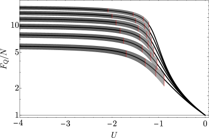
Figure 1: The QFI calculated with the ground state of the Hamiltonian (27) as a function of $U$ for $N=6,8,10,12,14,16$ (the higher the value reached at the plateau of $F_{q}=N^{2}$—i.e., the Heisenberg limit—the bigger the $N$) and normalized to the shot noise limit (shown with a grey line). On top of each curve we marked the regions where the correlator $\mathcal{E}_{N,0}$ detects at least $k$-partite nonlocality. Therefore, the darkest patch corresponds to $\mathcal{E}_{N,0}>\frac{1}{8}$, when all qubits are Bell-correlated. Next, when $\mathcal{E}_{N,0}\in]\frac{1}{16},\frac{1}{8}]$, so the nonlocality encompasses at least $N-1$ qubits, and so forth. The plot shows that the $F_{q}$ increases monotonously as the number of nonlocally correlated qubits grows. The red lines separating the regimes with different strength of nonlocality are added for clarity.

We now pick all the basis states $|n\rangle$ and $|m\rangle$, which are transformed one into another with given $\hat{\mathcal{R}}_{\vec{n}_{+}}$ and $\hat{\mathcal{L}}_{\vec{n}_{-}}$, leaving the other $N-(n_{+}+n_{-})$ qubits unaltered. We denote such set as $\mathcal{A}_{\vec{n}_{+},\vec{n}_{-}}$. A sum over all such $2^{N-(n_{+}-n_{-})}$ states has a common prefactor $(n_{\uparrow}-m_{\uparrow})^{2}=(n_{+}-n_{-})^{2}$. Note that if not for the modulus square in Eq. (13), such sum would represent a mean of the product of the two operators, namely

$$\sum_{n,m\in\mathcal{A}_{\vec{n}_{+},\vec{n}_{-}}}\!\!\!\!\!\!\!\!\!\varrho_{nm}={\rm Tr}\left[\hat{\varrho}\hat{\mathcal{R}}_{\vec{n}_{+}}\hat{\mathcal{L}}_{\vec{n}_{-}}\right].$$ (18)

Using

$$\sum_{i=1}^{n}|a_{i}|^{2}\geqslant\frac{1}{2^{n}}|\sum_{i=1}^{n}a_{i}|^{2}$$ (19)

which holds for any set of $2^{n}$ complex numbers (see Appendix D), we obtain

$$\sum_{n,m\in\mathcal{A}_{\vec{n}_{+},\vec{n}_{-}}}\!\!\!\!\!\!\!\!\!|\varrho_{nm}|^{2}\geqslant\frac{1}{2^{N-(n_{+}+n_{-})}}\mathcal{E}_{\vec{n}_{+},\vec{n}_{-}}$$ (20)

where in correspondence to Eq. (1) we introduced

$$\mathcal{E}_{\vec{n}_{+},\vec{n}_{-}}\vcentcolon=\big{|}{\rm Tr}\left[\hat{\varrho}\hat{\mathcal{R}}_{\vec{n}_{+}}\hat{\mathcal{L}}_{\vec{n}_{-}}\right]\big{|}^{2}.$$ (21)

We plug the inequality (20) into (13) and first sum over all possible combinations of fixed $n_{+}$ and $n_{-}$, and finally over all $n_{+}$ and $n_{-}$, obtaining the central expression of this work

$$F_{q}\geqslant 2\sum_{n_{+}=0}^{N}\sum_{n_{-}=0}^{N-n_{+}}\frac{(n_{+}-n_{-})^{2}}{2^{N-(n_{+}+n_{-})}}\sum_{\vec{n}_{+},\vec{n}_{-}}\mathcal{E}_{\vec{n}_{+},\vec{n}_{-}}.$$ (22)

Thus the QFI and hence the metrological sensitivity is lower-bounded by a combination of $\mathcal{E}_{\vec{n}_{+},\vec{n}_{-}}$, i.e, non-negative Bell correlators of all orders, with non-negative coefficients. For a pure separable state

$$|\psi\rangle=\bigotimes_{k=1}^{N}\frac{1}{\sqrt{2}}\left(|\uparrow\rangle_{k}+|\downarrow\rangle_{k}\right),$$ (23)

we have $\mathcal{E}_{\vec{n}_{+},\vec{n}_{-}}=\left(\frac{1}{4}\right)^{n_{+}+n_{-}}$ for all $\vec{n}_{+}$ and $\vec{n}_{-}$ (this is a consequence of the spin-permutation symmetry of this state). Hence, the inequality (19) [and thus (20)] is saturated. With this $\mathcal{E}_{\vec{n}_{+},\vec{n}_{-}}$ the sum over $\vec{n}_{\pm}$ in Eq. (22) can be evaluated, giving the shot-noise scaling of the QFI with the number of qubits $F_{q}=N$ [note that for pure states, also the inequality (7) is saturated, hence the “=” sign]. To beat the SNL, it is sufficient that correlators such as $\mathcal{E}_{\vec{n}_{+},\vec{n}_{-}}$ grow by any amount from the entanglement–threshold value $\mathcal{E}_{\vec{n}_{+},\vec{n}_{-}}=\left(\frac{1}{4}\right)^{n_{+}+n_{-}}$ He et al. (2011); Niezgoda et al. (2020), though not necessarily crossing the Bell limit $\mathcal{E}_{\vec{n}_{+},\vec{n}_{-}}=\left(\frac{1}{2}\right)^{n_{+}+n_{-}}$.

However, many-body nonlocality is sufficient (therefore it is a resource) to give ultra-high sensitivity. If $\mathcal{E}_{N,0}>\frac{1}{4}\frac{1}{2^{m+1}}$, at least $N-m$ qubits are Bell correlated (see Appendix A), and then Eq. (22) gives

$$F_{q}\geqslant\frac{N^{2}}{2^{m+1}}.$$ (24)

In particular, when all qubits are nonlocally correlated, then

$$F_{q}\geqslant\frac{N^{2}}{2}.$$ (25)

The extreme example is the Greenberger-Horne-Zeilinger (GHZ) state

$$|\psi\rangle=\frac{1}{\sqrt{2}}\left(\bigotimes_{k=1}^{N}|\uparrow\rangle_{k}+\bigotimes_{k=1}^{N}|\downarrow\rangle_{k}\right),$$ (26)

which gives $\mathcal{E}_{N,0}=\mathcal{E}_{0,N}=\frac{1}{4}$, (all $N$ qubits are Bell-correlated) and $F_{q}=N^{2}$.

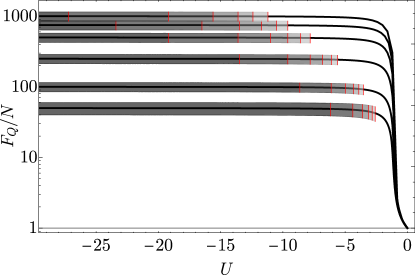
Figure 2: The QFI calculated with the ground state of the Hamiltonian (28) as a function of $U$ for $N=50,100,250,500,750,1000$ (the higher the plateau the bigger the $N$) and normalized to the shot noise limit. On top of each curve, the full $N$-body correlator of highest orders is presented with shades of gray, analogically to Fig. 1. For higher $N$, the Heisenberg level is approached even when $n<N$ qubits is nonlocally correlated.

We illustrate these general considerations with some physical examples. First, we take the anti-ferromagnetic Ising Hamiltonian with open boundary conditions, i.e.,

$$\hat{H}=U\sum_{j=1}^{N-1}\hat{\sigma}_{z}^{(j)}\hat{\sigma}_{z}^{(j+1)}-\sum_{j=1}^{N}\hat{\sigma}_{x}^{(j)}$$ (27)

where $U$ is the strength of the two-body interactions. We take $N=6,8,10,12,14$ and 16 and for each $N$ find the ground state for different $U<0$. For each $U$ we calculate the QFI using the formula (6) with the generator (9) aligned along the $\xi=z$ axis. On top of this, we evaluate the $N$-body correlator $\mathcal{E}_{N,0}$ and highlight the values of $U$ for which the correlator detects the many-body nonlocality of the growing order, see Fig. 1. Clearly, the growing depth of nonlocality is linked with approaching the Heisenberg limit, in accordance to Eq. (24).

As another prominent example we take the collection of $N$ interacting bosonic qubits, such as an ultra-cold Bose gas in a double-well trap. In the two-mode approximation, such a system can be depicted with the Hamiltonian

$$\hat{H}=-\hat{J}_{x}+U\hat{J}_{z}^{2},$$ (28)

where the collective spin operators $\hat{J}_{x}$ and $\hat{J}_{z}$ are given by Eq. (9) with $\xi=x$ and $\xi=z$ respectively. The ground state of this system undergoes a quantum phase transition as $U$ passes and drops below $-1$ Dziarmaga et al. (2002); Trenkwalder et al. (2016), and when $U\rightarrow-\infty$ the ground state approaches the GHZ state (26), which is well-suited for our purposes. Figure 2 shows the QFI as a function of $U$ for $N=50,100,250,500,750,1000$ and the correlator $\mathcal{E}_{N,0}$. Again, we observe that when $F_{q}\simeq N^{2}$, the system is highly nonlocal. When $N\gg 1$, the $F_{q}\simeq N^{2}$ plateau is reached even when $n<N$ qubits are nonlocally correlated because for large $N$, when a small number of qubits remains uncorrelated, the coefficient $(n_{+}-n_{-})^{2}$ from Eq. (22) is still close to $N^{2}$. This shows that for $N\rightarrow\infty$, while the many-body nonlocality remains sufficient to have high sensitivity, the correlation does not need to encompass all the qubits to have Heisenberg-like scaling.

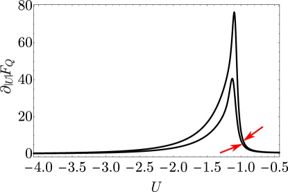
Figure 3: The derivative of QFI with respect to $U$ for $N=100$ (bottom) and $150$ (top), which shows a rapid growth of sensitivity around the point of quantum phase transition. The red arrows indicate the value of $U$ at which the Bell correlator starts to witness the nonlocality, $\mathcal{E}_{N,0}>\frac{1}{2^{N}}$.

Figure 3 shows the behaviour of the derivative of QFI over $|U|$ for $N=100$ and $N=150$. Around $U=-1$ point, the QFI starts to rapidly grow (large derivative) and this is accompanied by the emergence of Bell correlations, $\mathcal{E}_{N,0}>\frac{1}{2^{N}}$, as marked by red arrows. This further underlines the significance of nonlocality for quantum sensing and the peculiarity of the transition point.

In this work we have shown that a many-body nonlocality is a driving mechanism for ultra-precise metrology. We have expressed the quantum Fisher information in terms of a combination of a particular set of correlation functions of all orders—such that witness the nonlocality extending over many particles. This central result allowed to provide the lower bound for the sensitivity and identify the necessary condition to reach the Heisenberg scaling of the $F_{q}$. These general considerations were illustrated with some prominent examples of multi-qubit systems: a collection of spins forming an Ising chain and a gas of ultra-cold atoms in any two-mode configuration, for instance trapped in a double-well potential. Our findings shed some light on the highly non-classical properties of many-body systems and their applications.

We acknowledge the support of the National Science Centre, Poland under the QuantERA programme, Project no. 2017/25/Z/ST2/03039.

Appendix A Bounds for the correlator

The maximal value of the $N$-party Bell correlator is $\mathcal{E}_{N}=\frac{1}{4}$ Niezgoda et al. (2020) (here we do not specify the number of risen/lowered spins, for clarity of notation). If a single party (say, the first) is not nonlocally with the other, then

$$\mathcal{E}_{N}=|\langle\prod_{k=1}^{N}\sigma^{(k)}_{\pm}\rangle|^{2}\leqslant\int\!d\lambda\,p(\lambda)\,\mathcal{E}_{N-1}(\lambda)|\sigma^{(1)}_{\pm}(\lambda)|^{2},$$ (29)

where $\mathcal{E}_{N-1}$ is the $N-1$-party correlator, while $|\sigma^{(1)}_{\pm}(\lambda)|^{2}$ is calculated within the first subsystem. Since also $\mathcal{E}_{N-1}(\lambda)\leqslant\frac{1}{4}$, then the correlator (29) is upper-bounded by $\frac{1}{8}$. This procedure can be continued, and so when 2 parties are not nonlocally correlated, then $\mathcal{E}_{N}\leqslant\frac{1}{16}$. From this sequence of bounds it follows that when $\mathcal{E}_{N}>\frac{1}{8}$, all parties are Bell-correlated. If $\mathcal{E}_{N}>\frac{1}{16}$, at least $N-1$ are nonlocally correlated, and generally when $\mathcal{E}_{N}>\frac{1}{4}\frac{1}{2^{m+1}}$, then at least $N-m$ qubits are Bell-correlated.

Appendix B Derivation of the lower bound (8)

Starting from Eq. (7) from the main text, we sum over $j$ and obtain

$$F_{q} \geqslant 2\sum_{i}\langle\psi_{i}|[\hat{\varrho},\hat{h}][\hat{\varrho},\hat{h}]^{\dagger}|\psi_{i}\rangle=2\sum_{i}\langle\psi_{i}|(\hat{\varrho}\hat{h}-\hat{h}\hat{\varrho})(\hat{h}\hat{\varrho}-\hat{\varrho}\hat{h})|\psi_{i}\rangle=2\sum_{i}\langle\psi_{i}|(\hat{\varrho}\hat{h}^{2}\hat{\varrho}+\hat{h}\hat{\varrho}^{2}\hat{h}-\hat{\varrho}\hat{h}\hat{\varrho}\hat{h}-\hat{h}\hat{\varrho}\hat{h}\hat{\varrho})|\psi_{i}\rangle.$$ (30)

Now we consider each step separately.

$$\sum_{i}\langle\psi_{i}|\hat{\varrho}\hat{h}^{2}\hat{\varrho}|\psi_{i}\rangle=\sum_{i}p_{i}^{2}\langle\psi_{i}|\hat{h}^{2}|\psi_{i}\rangle={\rm Tr}\left[\hat{\varrho}^{2}\hat{h}^{2}\right].$$ (31a)

$$\sum_{i}\langle\psi_{i}|\hat{h}\hat{\varrho}^{2}\hat{h}|\psi_{i}\rangle=\sum_{i}\langle\psi_{i}|\hat{h}\sum_{j}p_{j}^{2}|\psi_{j}\rangle\!\langle\psi_{j}|\hat{h}|\psi_{i}\rangle=\sum_{j}p_{j}^{2}\langle\psi_{j}|\hat{h}^{2}|\psi_{j}\rangle={\rm Tr}\left[\hat{\varrho}^{2}\hat{h}^{2}\right].$$ (31b)

$$\sum_{i}\langle\psi_{i}|\hat{\varrho}\hat{h}\hat{\varrho}\hat{h}|\psi_{i}\rangle={\rm Tr}\left[(\hat{\varrho}\hat{h})^{2}\right]$$ (31c)

$$\sum_{i}\langle\psi_{i}|\hat{h}\hat{\varrho}\hat{h}\hat{\varrho}|\psi_{i}\rangle={\rm Tr}\left[\hat{h}\hat{\varrho}\hat{h}\hat{\varrho}\right]={\rm Tr}\left[\hat{\varrho}\hat{h}\hat{\varrho}\hat{h}\right]={\rm Tr}\left[(\hat{\varrho}\hat{h})^{2}\right].$$ (31d)

Therefore, the lower bound is

$$F_{q}\geqslant 4\left({\rm Tr}\left[\hat{\varrho}^{2}\hat{h}^{2}\right]-{\rm Tr}\left[(\hat{\varrho}\hat{h})^{2}\right]\right)$$ (32)

as quoted in the main text.

Appendix C Explicit formula for the lower bound

We now consider both terms of the lower bound (32) separately. First, we have

$${\rm Tr}\left[\hat{\varrho}^{2}\hat{h}^{2}\right] ={\rm Tr}\left[\hat{h}\hat{\varrho}^{2}\hat{h}\right]={\rm Tr}\left[\sum_{n,k,m}\left(n_{\uparrow}-\frac{N}{2}\right)\left(m_{\uparrow}-\frac{N}{2}\right)\varrho_{nk}\varrho_{km}|n\rangle\!\langle m|\right]=\sum_{n,m}\left(n_{\uparrow}-\frac{N}{2}\right)^{2}|\varrho_{nm}|^{2}.$$ (33)

The second term reads

$${\rm Tr}\left[(\hat{\varrho}\hat{h})^{2}\right] ={\rm Tr}\left[\hat{h}\hat{\varrho}\hat{h}\hat{\varrho}\right]={\rm Tr}\left[\sum_{n,m}\left(n_{\uparrow}-\frac{N}{2}\right)\left(m_{\uparrow}-\frac{N}{2}\right)\varrho_{nm}|n\rangle\!\langle m|\sum_{k,l}\varrho_{kl}|k\rangle\!\langle l|\right]$$

$$=\sum_{n,m}\left(n_{\uparrow}-\frac{N}{2}\right)\left(m_{\uparrow}-\frac{N}{2}\right)|\varrho_{nm}|^{2}.$$ (34)

Therefore, the lower bound for the QFI reads

$$F_{q}\geqslant 4\sum_{n,m}\left[\left(n_{\uparrow}-\frac{N}{2}\right)^{2}-\left(n_{\uparrow}-\frac{N}{2}\right)\left(m_{\uparrow}-\frac{N}{2}\right)\right]|\varrho_{nm}|^{2}=4\sum_{n,m}\left(n_{\uparrow}-\frac{N}{2}\right)(n_{\uparrow}-m_{\uparrow})|\varrho_{nm}|^{2}.$$ (35)

Now, by splitting this sum into two equal parts and in one of them exchanging the indices $n\leftrightarrow m$, we obtain

$$F_{q}\geqslant 2\sum_{n,m}\left(n_{\uparrow}-\frac{N}{2}\right)(n_{\uparrow}-m_{\uparrow})|\varrho_{nm}|^{2}+2\sum_{n,m}\left(m_{\uparrow}-\frac{N}{2}\right)(m_{\uparrow}-n_{\uparrow})|\varrho_{mn}|^{2}.$$ (36)

Since $|\varrho_{mn}|^{2}=|\varrho_{nm}|^{2}$ we obtain the final expression

$$F_{q}\geqslant 2\sum_{n,m}(n_{\uparrow}-m_{\uparrow})^{2}|\varrho_{nm}|^{2}.$$ (37)

Appendix D Proof for the algebraic inequality

Here we prove that

$$\sum_{i=1}^{2^{n}}|a_{i}|^{2}\geqslant\frac{1}{2^{n}}\Big{|}\sum_{i=1}^{2^{n}}a_{i}\Big{|}^{2},$$ (38)

for any set of complex numbers $\{a_{1}\ldots a_{2^{n}}\}$. To this end, note that for $n=1$ we have

$$|a_{1}|^{2}+|a_{2}|^{2}=\frac{1}{2}\left(|a_{1}+a_{2}|^{2}+|a_{1}-a_{2}|^{2}\right)\geqslant\frac{1}{2}|a_{1}+a_{2}|^{2}.$$ (39)

Similarly, for $n=2$

$$|a_{1}|^{2}+|a_{2}|^{2}+|a_{3}|^{2}+|a_{4}|^{2}=$$

$$=\frac{1}{4}\left(|a_{1}+a_{2}+(a_{3}+a_{4})|^{2}+|a_{1}+a_{2}-(a_{3}+a_{4})|^{2}+|a_{1}-a_{2}+(a_{3}-a_{4})|^{2}+|a_{1}-a_{2}-(a_{3}-a_{4})|^{2}\right)$$

$$\geqslant\frac{1}{4}|a_{1}+a_{2}+a_{3}+a_{4}|^{2}.$$ (40)

It is now clear how to proceed for higher $n$. First, the full expression is divided into two halves, namely

$$b_{1}=\sum_{i=1}^{2^{n-1}}a_{i},\ \ \ b_{2}=\sum_{i=1}^{2^{n-1}}a_{i+2^{n-1}}$$ (41)

and we apply the formula (39) with $a_{1}$ and $a_{2}$ replaced with $b_{1}$ and $b_{2}$. Next, a minus sign must be inserted in the middle of $b_{1}$ and $b_{2}$, giving

$$c_{1}=\sum_{i=1}^{2^{n-2}}a_{i}-\sum_{i=1}^{2^{n-2}}a_{i+2^{n-2}},$$ (42)

$$c_{2}=\sum_{i=1}^{2^{n-2}}a_{i+2^{n-1}}-\sum_{i=1}^{2^{n-2}}a_{i+2^{n-1}+2^{n-2}}.$$ (43)

This procedure is iterated a total of $2^{n}$ times, giving $2^{n}$ terms

$$\sum_{i=1}^{2^{n}}|a_{i}|^{2}=\frac{1}{2^{n}}( |b_{1}+b_{2}|^{2}+|b_{1}-b_{2}|^{2}$$ (44)

$$+|c_{1}+c_{2}|^{2}+|c_{1}-c_{2}|^{2}+\ldots).$$ (45)

By neglecting all the terms apart from the first one, we obtain the inequality (38).

References

• Horodecki et al. (2009) R. Horodecki, P. Horodecki, M. Horodecki,  and K. Horodecki, Rev. Mod. Phys. 81, 865 (2009).
• Einstein et al. (1935) A. Einstein, B. Podolsky,  and N. Rosen, Phys. Rev. 47, 777 (1935).
• He et al. (2012) Q. Y. He, P. D. Drummond, M. K. Olsen,  and M. D. Reid, Phys. Rev. A 86, 023626 (2012).
• Cavalcanti et al. (2009) E. G. Cavalcanti, S. J. Jones, H. M. Wiseman,  and M. D. Reid, Phys. Rev. A 80, 032112 (2009).
• Bell (1964) J. S. Bell, Physics 1, 195 (1964).
• Brunner et al. (2014) N. Brunner, D. Cavalcanti, S. Pironio, V. Scarani,  and S. Wehner, Rev. Mod. Phys. 86, 419 (2014).
• Ekert (1991) A. K. Ekert, Phys. Rev. Lett. 67, 661 (1991).
• Chun-Yan et al. (2005) L. Chun-Yan, Z. Hong-Yu, W. Yan,  and D. Fu-Guo, Chinese Physics Letters 22, 1049 (2005).
• Barrett et al. (2005) J. Barrett, L. Hardy,  and A. Kent, Phys. Rev. Lett. 95, 010503 (2005).
• Acín et al. (2006) A. Acín, N. Gisin,  and L. Masanes, Phys. Rev. Lett. 97, 120405 (2006).
• Gisin et al. (2010) N. Gisin, S. Pironio,  and N. Sangouard, Phys. Rev. Lett. 105, 070501 (2010).
• Sørensen and Mølmer (2000) A. Sørensen and K. Mølmer, Phys. Rev. A 62, 022311 (2000).
• Chen et al. (2014) M. Chen, N. C. Menicucci,  and O. Pfister, Phys. Rev. Lett. 112, 120505 (2014).
• Giovannetti et al. (2004) V. Giovannetti, S. Lloyd,  and L. Maccone, Science 306, 1330 (2004).
• Pezzé and Smerzi (2009) L. Pezzé and A. Smerzi, Phys. Rev. Lett. 102, 100401 (2009).
• Yadin et al. (2020) B. Yadin, M. Fadel,  and M. Gessner, arXiv preprint arXiv:2009.08440  (2020).
• Fröwis et al. (2019) F. Fröwis, M. Fadel, P. Treutlein, N. Gisin,  and N. Brunner, Phys. Rev. A 99, 040101 (2019).
• Niezgoda et al. (2019) A. Niezgoda, J. Chwedeńczuk, L. Pezzé,  and A. Smerzi, Phys. Rev. A 99, 062115 (2019).
• Freedman and Clauser (1972) S. J. Freedman and J. F. Clauser, Phys. Rev. Lett. 28, 938 (1972).
• Aspect et al. (1981) A. Aspect, P. Grangier,  and G. Roger, Phys. Rev. Lett. 47, 460 (1981).
• Aspect et al. (1982) A. Aspect, J. Dalibard,  and G. Roger, Phys. Rev. Lett. 49, 1804 (1982).
• Tittel et al. (1998a) W. Tittel, J. Brendel, B. Gisin, T. Herzog, H. Zbinden,  and N. Gisin, Phys. Rev. A 57, 3229 (1998a).
• Tittel et al. (1998b) W. Tittel, J. Brendel, H. Zbinden,  and N. Gisin, Phys. Rev. Lett. 81, 3563 (1998b).
• Weihs et al. (1998) G. Weihs, T. Jennewein, C. Simon, H. Weinfurter,  and A. Zeilinger, Phys. Rev. Lett. 81, 5039 (1998).
• Pan et al. (2000) J.-W. Pan, D. Bouwmeester, M. Daniell, H. Weinfurter,  and A. Zeilinger, Nature 403, 515 (2000).
• Kielpinski et al. (2001) D. Kielpinski, V. Meyer, C. A. Sackett, W. M. Itano, C. Monroe,  and D. J. Wineland, Nature 409, 791 (2001).
• Gröblacher et al. (2007) S. Gröblacher, T. Paterek, R. Kaltenbaek, Č. Brukner, M. Żukowski, M. Aspelmeyer,  and A. Zeilinger, Nature 446, 871 (2007).
• Salart et al. (2008) D. Salart, A. Baas, J. A. W. van Houwelingen, N. Gisin,  and H. Zbinden, Phys. Rev. Lett. 100, 220404 (2008).
• Hensen et al. (2015) B. Hensen, H. Bernien, A. Dréau, A. Reiserer, N. Kalb, M. Blok, J. Ruitenberg, R. Vermeulen, R. Schouten, C. Abellán, et al., Nature 526, 682 (2015).
• Ansmann et al. (2009) M. Ansmann, H. Wang, R. C. Bialczak, M. Hofheinz, E. Lucero, M. Neeley, A. D. O’Connell, D. Sank, M. Weides, J. Wenner, A. N. Cleland,  and J. M. Martinis, Nature 461, 504 (2009).
• Lamehi-Rachti and Mittig (1976) M. Lamehi-Rachti and W. Mittig, Phys. Rev. D 14, 2543 (1976).
• Rosenfeld et al. (2017) W. Rosenfeld, D. Burchardt, R. Garthoff, K. Redeker, N. Ortegel, M. Rau,  and H. Weinfurter, Phys. Rev. Lett. 119, 010402 (2017).
• Schmied et al. (2016) R. Schmied, J.-D. Bancal, B. Allard, M. Fadel, V. Scarani, P. Treutlein,  and N. Sangouard, Science 352, 441 (2016).
• Shin et al. (2019) D. K. Shin, B. M. Henson, S. S. Hodgman, T. Wasak, J. Chwedeńczuk,  and A. G. Truscott, Nature Communications 10, 4447 (2019).
• Gross et al. (2010) C. Gross, T. Zibold, E. Nicklas, J. Esteve,  and M. K. Oberthaler, Nature 464, 1165 (2010).
• Riedel et al. (2010) M. F. Riedel, P. Böhi, Y. Li, T. W. Hänsch, A. Sinatra,  and P. Treutlein, Nature 464, 1170 (2010).
• Leroux et al. (2010) I. D. Leroux, M. H. Schleier-Smith,  and V. Vuletić, Phys. Rev. Lett. 104, 250801 (2010).
• Chen et al. (2011) Z. Chen, J. G. Bohnet, S. R. Sankar, J. Dai,  and J. K. Thompson, Phys. Rev. Lett. 106, 133601 (2011).
• Esteve et al. (2008) J. Esteve, C. Gross, A. Weller, S. Giovanazzi,  and M. Oberthaler, Nature 455, 1216 (2008).
• Strobel et al. (2014) H. Strobel, W. Muessel, D. Linnemann, T. Zibold, D. B. Hume, L. Pezzé, A. Smerzi,  and M. K. Oberthaler, Science 345, 424 (2014).
• Braunstein and Caves (1994) S. L. Braunstein and C. M. Caves, Phys. Rev. Lett. 72, 3439 (1994).
• Brush (1967) S. G. Brush, Rev. Mod. Phys. 39, 883 (1967).
• Baxter (2016) R. J. Baxter, Exactly solved models in statistical mechanics (Elsevier, 2016).
• Dalfovo et al. (1999) F. Dalfovo, S. Giorgini, L. P. Pitaevskii,  and S. Stringari, Reviews of Modern Physics 71, 463 (1999).
• Shin et al. (2004) Y. Shin, M. Saba, T. Pasquini, W. Ketterle, D. Pritchard,  and A. Leanhardt, Physical review letters 92, 050405 (2004).
• Gati et al. (2006) R. Gati, B. Hemmerling, J. Fölling, M. Albiez,  and M. K. Oberthaler, Phys. Rev. Lett. 96, 130404 (2006).
• Cavalcanti et al. (2007) E. G. Cavalcanti, C. J. Foster, M. D. Reid,  and P. D. Drummond, Phys. Rev. Lett. 99, 210405 (2007).
• He et al. (2011) Q. He, P. Drummond,  and M. Reid, Physical Review A 83, 032120 (2011).
• Cavalcanti et al. (2011) E. Cavalcanti, Q. He, M. Reid,  and H. Wiseman, Physical Review A 84, 032115 (2011).
• Niezgoda et al. (2020) A. Niezgoda, M. Panfil,  and J. Chwedeńczuk, Phys. Rev. A 102, 042206 (2020).
• Dziarmaga et al. (2002) J. Dziarmaga, A. Smerzi, W. Zurek,  and A. Bishop, Physical review letters 88, 167001 (2002).
• Trenkwalder et al. (2016) A. Trenkwalder, G. Spagnolli, G. Semeghini, S. Coop, M. Landini, P. Castilho, L. Pezze, G. Modugno, M. Inguscio, A. Smerzi, et al., Nature physics 12, 826 (2016).