Entanglement order parameters and critical behavior for topological phase transitions and beyond

Abstract

Order parameters are key to our understanding of phases of matter. Not only do they allow to classify phases, but they also enable the study of phase transitions through their critical exponents which identify the universal long-range physics underlying the transition. Topological phases are exotic quantum phases which are lacking the characterization in terms of order parameters. While probes have been developed to identify such phases, those probes are only qualitative in that they take discrete values, and thus provide no means to study the scaling behavior in the vicinity of phase transitions. In this paper, we develop a unified framework based on variational tensor networks (infinite Projected Entangled Pair States, or iPEPS) for the quantitative study of both topological and conventional phase transitions through entanglement order parameters. To this end, we employ tensor networks with suitable physical and/or entanglement symmetries encoded, and allow for order parameters detecting the behavior of any of those symmetries, both physical and entanglement ones. On the one hand, this gives rise to entanglement-based order parameters for topologically ordered phases. These topological order parameters allow to quantitatively probe the behavior when going through topological phase transitions and thus to identify universal signatures of such transitions. We apply our framework to the study of the Toric Code model in different magnetic fields, which along some special lines maps to the (2+1)D Ising model. Our method identifies 3D Ising critical exponents for the entire transition, consistent with those special cases and general belief. However, we in addition also find an unknown critical exponent $\beta^{*}\approx 0.021$ for one of our topological order parameters. We take this – together with known dualities between Toric Code and Ising model – as a motivation to also apply our framework of entanglement order parameters to conventional phase transitions. There, it enables us to construct a novel type of disorder operator (or disorder parameter), which is non-zero in the disordered phase and measures the response of the wavefunction to a symmetry twist in the entanglement. We numerically evaluate this disorder operator for the (2+1)D transverse field Ising model, where we again recover a critical exponent hitherto unknown in the (2+1)D Ising model, $\beta^{*}\approx 0.024$, consistent with the findings for the Toric Code. This shows that entanglement order parameters can provide additional means of characterizing the universal data both at topological and conventional phase transitions, and altogether demonstrates the power of this framework to identify the universal data underlying the transition.

I Introduction

Symmetries play a central role in modern physics. In particular, they are the key to understand the way in which many-body systems, both classical and quantum, organize themselves into different phases, a problem central to condensed matter physics, high-energy physics, and beyond. To this end, one needs to consider the full set of symmetries of the interactions which describe a system at hand, and study whether its state obeys the same symmetries or chooses to break some of them. This can be captured through local order parameters which are chosen such as to detect a breaking of the symmetry. The understanding in terms of symmetries and order parameters, however, does not only enable us to classify the ways in which many-body systems can order, but it moreover allows to quantitatively assess how the system behaves as it undergoes a phase transition, which forms the heart of Landau theory. Indeed, the scaling behavior of the order parameter in the vicinity of a phase transition allows to extract the universal features of the transition, that is, the fingerprint of its long-range physics; it is a most notable fact that phase transitions in scenarios such different as liquid-gas or magnetic transitions fall into the same few universality classes, which in turn allows to use effective field theories to capture the universal long-range physics.

Topological phases are zero-temperature phases of quantum many-body systems which fall outside of the Landau paradigm [1, 2]. They exhibit ordering, witnessed e.g. by a non-trivial ground space degeneracy and excitations with a non-trivial statistics (“anyons”). Yet, those ground states, and thus the topological phase itself, cannot be characterized by any local order parameter. Instead, other probes for identifying topologically non-trivial states have been developed, such as a universal constant correction $\gamma$ to the area-law scaling of the entanglement entropy, $S(A)=c|A|-\gamma$ [3, 4], features of the entanglement spectrum [5], or properties extracted from a full set of “minimally entangled” ground states which carry information about the statistics of the excitations [6].

Yet, all these probes for topological order suffer from a severe shortcoming as compared to conventional order parameters: On the one hand, conventional order parameters allow to identify the phase at hand – they are qualitative order parameters. But at the same time, they also allow to quantitatively study the behavior of the system as it undergoes a phase transition, and to extract information about the universal properties of the transition – they are quantitative order parameters. While fingerprints for topological order such as the topological correction $\gamma$ or anyon statistics are qualitative order parameters for topological phases, they can only take a discrete set of values by construction and thus cannot be used for a quantitative study of topological phase transitions. This leaves the quantitative study of topological phase transitions wide open, with information about the underlying universal behavior limited to cases where exact [7] or approximate [8] duality mappings to other known models can be devised, or where universal signatures can be extracted from the scaling of the bulk gap [9] or the CFT structure of the full entanglement spectrum of the 2D bulk at criticality [10].

In this paper, we develop a framework for the quantitative study of topological phase transitions through order parameters based on tensor networks, specifically iPEPS [11, 12, 13]. Given a lattice model $H$, our method uses variationally optimized iPEPS wavefunctions to construct order parameters which characterize the topological features of the system, namely the behavior of the topological quasi-particles (anyons) and the way in which they cease to exist at the phase transition, that is, their condensation and confinement. Unlike other signatures of topological order, these order parameters vanish continuously as the phase transition is approached and thus allow for the extraction of critical exponents which enable the microscopic study of topological phase transitions and the verification and identification of their universal behavior.

We apply our framework to the study of the Toric Code model in a simultaneous $x$ and $z$ magnetic field, where we use it to extract different critical exponents which characterize the transition. On the one hand, we recover the anticipated 3D Ising critical exponents $\beta$ (for the order parameter) and $\nu$ (for diverging lengths), consistent with previous evidence found for the 3D Ising universality class [7, 8, 9]. For the order parameter for deconfinement, however, we find a new and yet unknown critical exponent $\beta^{*}\approx 0.021$. Our framework thus allows to extract the universal signatures of topological phase transitions, but even goes further and provides access to additional critical exponents.

The observation of a yet unknown critical exponent, together with the well-known duality mapping between the Toric Code with a pure $x$ or $z$ field and the (2+1)D transverse field Ising model, motivates us to investigate whether similar techniques can also be used to set up disorder parameters for conventional phase transitions, such as for the (2+1)D Ising model, and whether those exhibit those unknown critical exponents as well.

We therefore consider symmetry breaking phase transitions, which we simulate variationally using iPEPS with the global symmetry encoded in the tensor. We propose to use the response of the variational wavefunction to the insertion of a “symmetry twist” on the entanglement degrees of freedom as a disorder parameter, as we show that a non-zero value implies being in the disordered phase. We study the proposed disorder parameter numerically for the (2+1)D Ising model, and find a critical exponent $\beta^{*}\approx 0.024$ (consistent with the Toric Code result up to numerical precision), in agreement with the expected duality mapping. Our construction therefore constitutes a novel way to define disorder parameters for conventional phases, which provide a new tool to extract additional signatures of universal behavior at criticality from the system. Notably, this construction intrinsically relies on the description of the system in terms of symmetric PEPS, which gives access to properties which cannot be captured in a direct way by probing the physical degrees of freedom alone.

In order to achieve the goals of the paper, we build on a number of ingredients. First, we exploit that iPEPS form a powerful framework for the simulation of strongly correlated quantum spin systems, based on the description of a complex entangled many-body wavefunction in terms of local tensors which flesh out the interplay of locality and entanglement, and we make use of the powerful variational algorithms developed for iPEPS [14, 15, 16, 17]. Next, we exploit the key role played by entanglement symmetries in describing topologically ordered systems: While these symmetries had originally been identified in explicitly constructed model wavefunctions with topological order [18, 19, 20, 21], they have recently also been found to show up in variationally optimized wavefunctions for topologically ordered systems [22]; they thus constitute the right structure for the description of topologically ordered systems. We thus impose the corresponding symmetries when variationally optimizing the iPEPS tensor. Next, these symmetries are known to allow to model anyons and study their behavior in explicitly constructed wavefunction families [18, 20, 23, 24, 25, 26, 27]. A key step of our work is to show that it is possible to generalize this description to the case of variationally optimized iPEPS. In particular, this requires a careful consideration of the way in which order parameters are constructed solely based on the symmetries present, without any further information at hand. While this seems contrived for regular order parameters (where the full Hamiltonian and its dependence on external parameters such as magnetic fields is known) and for explicitly constructed PEPS model wavefunctions (where the full tensor and its parameter dependence are given explicitly), this turns out to be crucial for variationally optimizied iPEPS, where we have no information available but the symmetry itself; a significant part of the manuscript deals with this discussion.

The remainder of the paper is structured as follows: In Sec. II, we develop our framework for the construction of order parameters in topological phases. In Sec. III, we apply our method to the in-depth study of the Toric Code model in different magnetic fields. Finally, in Sec. V, we discuss some further aspects of the method, before concluding in Sec. VI.

II Construction of topological order parameters

In this section, we describe how to construct and measure topological order parameter using iPEPS. We start in Sec. II.1 with an introduction to iPEPS, a discussion of entanglement symmetries, and the way in which those symmetries underly topological order and how they can be used to construct anyonic operators at the entanglement level. In Sec. II.2 we discuss the different physical behavior which those anyonic operators can display, and their relation to the topological phase the system exhibits.

The following two sections, II.3 and II.4, form the theoretical core of the construction of topological order parameters: We develop the framework of how to use anyonic operators to construct order parameters. The key challenge is that this construction must be based on the weakest possible assumption, namely that we only know about the symmetry of the model at hand, without any other information about the problem. This is since we describe the system by variationally optimized iPEPS tensors on which we only impose the entanglement symmetry – thus, the way the symmetry acts is the only information which we can be certain about, while all other degrees of freedom are subject to arbitrary gauge choices. While such a situation seems contrived in the case of an actual model where a concrete Hamiltonian is given, the study of order parameters based solely on the underlying symmetry can nevertheless be discussed in that general scenario, where it provides insights on their own right. Specifically, in Sec. II.3 we discuss how from symmetry considerations, we can connect anyonic order parameters to conventional and string order parameters in one dimension, and how symmetries underly the construction of the latter; and in Sec. II.4, we discuss the additional obstacles which appear when transitioning to the case where we want to use order parameters for the quantitative study of phase transitions. There, knowledge of the symmetry alone seems insufficient due to the free (and a priori random) gauge degrees of freedom, and we explain how this can be overcome by constructing order parameters which are gauge invariant, as well as through the introduction of suitable gauge fixing procedures.

Finally, in Sec. II.5, we provide a succinct and detailed technical recipe for how to measure topological order parameters in practice.

II.1 iPEPS, entanglement symmetries, and topological order

We start by introducing infinite Projected Entangled Pair States (iPEPS) [11, 12, 13]. For simplicity, we restrict to square lattices; other geometries can be accommodated either by adapting the lattice geometry or by blocking sites. We denote the physical dimension per site (possibly blocked) by $d$. An iPEPS of bond dimension $D$ is given by a five-index tensor

$$A\equiv A^{i}_{\alpha\beta\gamma\delta}=\quad\raisebox{-19.91684pt}{\includegraphics{Aten}}\quad,$$ (1)

with physical index $i=1,\dots,d$, and virtual indices $\alpha,\beta,\gamma,\delta=1,\dots,D$. It describes a wavefunction on an infinite plane by arranging the tensor on a square grid and contracting connected indices (that is, identifying and summing over them), depicted as

$$\raisebox{-19.91684pt}{\includegraphics{peps}}\ .$$ (2)

More formally, this contraction should be thought of as placing some suitable boundary conditions at the virtual indices at the boundary and taking those boundaries to infinity; numerically, this amounts to convergence of bulk properties independent of the chosen boundary conditions (except for possibly selecting a symmetry broken sector).

iPEPS form a powerful variational ansatz, as their entanglement structure (built up through the contraction of the virtual indices) is well suited to describe low-energy states of correlated quantum many-body systems, and there exists a range of algorithms to find the variationally optimal state for a given Hamiltonian [14, 15, 16, 17]. At the same time, they can be used to exactly capture a range of interesting wavefunctions, in particular renormalization fixed point (RGFP) models with (non-chiral) topological order, as well as models with finite correlation length through suitable deformations of the RGFP models.

A key point of the PEPS ansatz is that there is a gauge ambiguity: Two tensors which are related by a gauge

$$\raisebox{-19.91684pt}{\includegraphics{gaugesym}}\ ,$$ (3)

(with gauges $Q$ and $R$) describe the same wavefunction, as the gauges cancel in the contraction (2). In particular, for PEPS which have been obtained from a variational optimization rather than having been constructed explicitly – that is, those which are at the focus of this work – we cannot assume a specific gauge, and picking a suitable gauge will be of key importance later on.

PEPS models with topological order are characterized by an entanglement symmetry which is closely tied to their topological features. This symmetry shows up in all known model wavefunctions with topological order, but has recently also been found to appear in variational optimized tensors, and is thus naturally linked to topological order [18, 19, 20, 21, 22]. In the case of quantum doubles of finite groups $G$ [28] (which will be the focus of this work), this entanglement symmetry is given by

$$\raisebox{-19.91684pt}{\includegraphics{Ginjective}}\ ,$$ (4)

where $V_{g}$, $g\in G$, is some unitary representation of $G$ [18]. (In the graphical calculus, the $V_{g}$ are understood as $2$-index tensors which are accordingly contracted with the virtual indices.) Eq. (4) implies a “pulling through” property: Strings formed by $V_{g}$ (or $V_{g}^{\dagger}$, depending on the relative orientation of the string and the lattice) can be freely deformed, e.g.

(5)

For simplicity, in the following we will denote the $V_{g}$’s (or $V_{g}^{\dagger}$) by blue dots, if needed labelled by placing the group element $g$ next to it.

Restricting to tensors with a fixed symmetry (4), as we will do in our variational simulations, also induces a corresponding symmetry constraint on the gauge degrees of freedom (3): In order for the symmetry condition (4) to be preserved, we must have that

$$V_{g}QV_{g}^{\dagger}=Q\mbox{\quad and\quad}V_{g}RV_{g}^{\dagger}=R\ .$$ (6)

Figure 1: (a) Strings of symmetry operations $g\equiv V_{g}$, Eq. (4), possibly dressed by trivially transforming endpoints $C$, form pairs of magnetic fluxes. (b) Objects which transform as non-trivial irreducible representations $\alpha$ under $V_{g}$ form electric excitations, such as site tensors $B_{\alpha}$, or matrices $X_{\alpha}$ placed on links; again, they can be dressed with some trivially transforming tensor $C$. (c) A general pair of anyonic excitations, as used in this work to study anyon condensation and deconfinement. (d) Braiding as described in the language of entanglement symmetries (4) (see text).

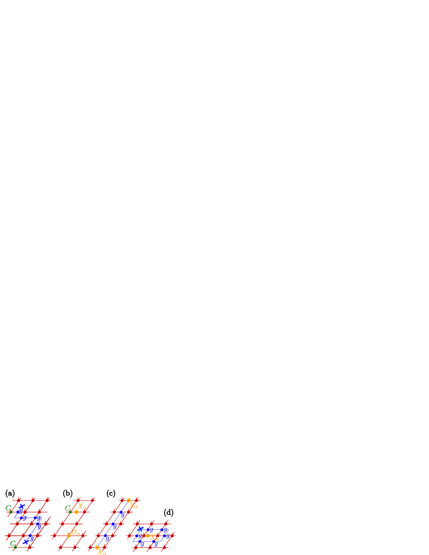
As it turns out, condition (5) is closely tied to topological order; in the following, we will focus on the case of Abelian groups $G$ for simplicity. First, we can use condition (5) to for instance parametrize a ground space manifold with a topological degeneracy, by wrapping strings of $V_{g}$ around the torus – as those strings are movable, they cannot be detected locally. Second, a string with two open ends – see Fig. 1a – allows to describe paired excitations: While the string itself can be moved using (4) and is thus not detectable, its endpoints (which are plaquettes with an odd number of adjacent $V_{g}$’s) cannot be moved, and we would thus expect them to be detectable; these correspond to magnetic excitations. On the other hand, replacing a tensor by one with a non-trivial transformation property

(7)

where $\alpha(g)$ is an irreducible representation of $G$ (or, alternatively, placing a matrix $X_{\alpha}$ with transformation property

$$V_{g}X_{\alpha}V_{g}^{\dagger}=\alpha(g)X_{\alpha}$$ (8)

on a bond) – see Fig. 1b – also yields a topological excitation: As it carries a total irrep charge under the action of $V_{g}$, it must come in charge-neutral pairs on a torus (or otherwise be compensated by the boundary conditions). Objects of this form are electric excitations. For both these types of excitations, or combinations of electric and magnetic excitations (“dyons”), we can additionally dress the endpoint with a trivially transforming tensor $C$ (i.e., one which satisfies (4)), e.g. to create an exact energy eigenstate. The most general pair of excitations (without the dressing) is shown in Fig. 1c.

When seen on the entanglement degrees of freedom, these objects carry all properties expected from anyonic excitations. They can only be created in pairs, and if we assume for a moment that we have a way to move and probe them, they exhibit precisely the statistics of the anyons in the double model $D(G)$. Most importantly, creating a pair of magnetic excitations for some $g\in G$, moving them around an electric excitation $\alpha$, and annihilating them again leaves us with a loop of $V_{g}$’s around $X_{\alpha}$, and thus yields a non-trivial braiding phase equal to $\alpha(g)$, following Eq. (8), illustrated in Fig. 1d.

For the RGFP model, where the tensor – up to a basis transformation on the physical system – is nothing but a projector onto the invariant space of the symmetry (4), these anyon-like objects on the entanglement level are mapped one-to-one to the physical level at the RGFP, that is to say, they can be created (in pairs), manipulated, and detected by local physical operations (the operations just need to respect the global $V_{g}$-symmetry). Thus, at the RGFP, these objects on the entanglement level describe real anyons, that is, localized excitations (quasi-particles) which are eigenstates of the Hamiltonian and have anyonic statistics. These excitations are characterized by a group element $g$ and an irreducible representation $\alpha$, and we will label them by $a\equiv(g,\alpha)$, and its anti-particle by $\bar{a}\equiv(g^{-1},\bar{\alpha})$ (here, $\bar{\alpha}$ denotes the complex conjugate).

II.2 Behavior of anyonic operators vs. topological order

Do the objects which we have just constructed necessarily describe topological excitations? They certainly possess the right properties at the entanglement level (we will call them “virtual anyons”), but does this necessarily mean they also describe proper physical anyons? As just argued, at the RGFP this can easily be seen to be the case, due to the unitary correspondence between the entanglement and physical degrees of freedom on the invariant subspace (4) – thus, the anyonic operators at the entanglement level can be created, manipulated, and detected by physical unitaries. This continues to holds as we move away from the RGFP – we can understand this e.g. using quasi-adiabatic evolution [29], which effectively evolves the tensors without affecting the entanglement symmetry (4), and which will thus only dress the endpoints of the strings (as in Fig. 1ab). In fact, this is precisely what underlies e.g. the excitation ansatz for topological excitations [30, 31]. Without this dressing of the endpoint, our virtual anyons might not be eigenstates of the Hamiltonian, but they will regardless describe an excitation in the corresponding topological sector (that is, a dispersing superposition of anyonic excitation with identical anyonic quantum number).

However, if we deform our tensors sufficiently strongly (e.g. towards a product state), even while keeping the symmetry (4), topological order will eventually break down. Yet, on the entanglement level, the “anyonic operators” still possess the same properties [32]. This raises the question: How can we determine whether the virtual anyons in Fig. 1c do indeed describe actual physical anyons? Or, equivalently, when is a system whose wavefunction is described by tensors with a symmetry (4) truly topologically ordered?

As it turns out, whether the system is topologically ordered, and whether the virtual anyons represent physical anyons, is precisely reflected in two properties, which we naturally demand from true anyonic excitations.
Properties of anyonic excitations: To define the properties we require from anyonic excitations in the topological phase, let us normalize our tensors such that the state is normalized on the infinite plane,

$$\langle\Omega|\Omega\rangle=1\ ,$$ (9)

and let us denote by $|\Psi_{a\bar{a}}(\ell)\rangle$ the state with a pair of “virtual anyons” $a$ and $\bar{a}$, Fig. 1c, placed at the entanglement degrees of freedom at separation $\ell$. We require the following properties from this state to describe a pair of physical anyons.

1. We need to be able to construct a well-defined, normalizable wavefunction with individual anyons at arbitrary locations. This is measured by the quantity

   $$N_{a\bar{a}}(\ell):=\langle\Psi_{a\bar{a}}(\ell)|\Psi_{a\bar{a}}(\ell)\rangle\ .$$ (10)

   For well-defined anyonic excitations, we require $N_{a\bar{a}}(\ell)\to K_{a}^{2}\neq 0$ as $\ell\to\infty$, such that $|\Psi_{a\bar{a}}\rangle$ is normalizable for arbitrarily separated anyonic excitations.

2. Individual anyonic excitations must be orthogonal to the ground state, as they are characterized by a non-trivial topological quantum number, i.e., they live in a different (global) symmetry sector. This is quantified by the overlap

   $$F_{a\bar{a}}(\ell):=\big{|}\langle\Psi_{a\bar{a}}(\ell)|\Omega\rangle\big{|}^{2}\ .$$ (11)

   We thus require that for non-trivial anyons $a$, $F_{a\bar{a}}(\ell)\to 0$ as $\ell\to\infty$. (As long as the anyons are close to each other, the total object $a\bar{a}$ has a trivial topological quantum number and can thus have a non-zero overlap with the ground state.)

Note that $0\leq F_{a\bar{a}}(\ell)\leq N_{a\bar{a}}(\ell)$, where the second inequality is the Cauchy-Schwarz inequality. It is thus natural to define a normalized quantity

$$\hat{F}_{a\bar{a}}(\ell):=F_{a\bar{a}}(\ell)/N_{a\bar{a}}(\ell)\leq 1\ .$$ (12)

In which way can the above two properties break down? First, we can have that for some anyon $a$, $N_{a\bar{a}}(\ell)\to 0$ as $\ell\to\infty$, that is, we are unable to construct a well-defined state as we separate the anyons $a$ and $\bar{a}$. In that case, we will say that the anyons $a$ and $\bar{a}$ are confined. This implies that also $F_{a\bar{a}}(\ell)\to 0$. Second, we can have that for some anyon $a$, $F_{a\bar{a}}(\ell)\to C_{a}^{2}>0$ (and thus also $N_{a\bar{a}}(\ell)\to K_{a}^{2}>0$). In that case, the “anyon” $a$ is no longer orthogonal to the ground state, that is, it is no longer characterized by a distinct topological quantum number and thus has condensed into the ground state.

We thus see that we for each “virtual anyon” $a$ constructed from the entanglement symmetry and its antiparticle $\bar{a}$, we have three distinct possibilities:

1. Free anyon: $N_{a\bar{a}}\to K_{a}^{2}>0$, $F_{a\bar{a}}\to 0$.

2. Confined anyon: $N_{a\bar{a}}\to 0$.

3. Condensed anyon: $\hat{F}_{a\bar{a}}\!\to\!\hat{C}_{a}^{2}\!>\!0$, $N_{a\bar{a}}\!\to\!K_{a}^{2}>0$.

We call $\hat{F}_{a\bar{a}}$ the condensate fraction and $N_{a\bar{a}}$ the deconfinement fraction for anyon $a$.

It turns out that these different behaviors can be used to identify the different topological phases (including the trivial phase) compatible with a given entanglement symmetry (4) with symmetry group $G$. In fact, it has been shown to be in one-to-one correspondence to the possible phases which can be obtained by the framework of anyon condensation from the quantum double model $D(G)$.

II.3 Anyonic operators as qualitative order parameters

As we have seen, the asymptotic behavior of $N_{a\bar{a}}(\ell)\to K_{a}^{2}$ and $F_{a\bar{a}}(\ell)\to C_{a}^{2}$ can serve as order parameters which allow to distinguish different topological and trivial phases. Let us now see how they can be related to conventionally defined order parameters and string order parameters [24, 33]. This will not only be insightful on its own right, but also provide us with guidance on how to use them as starting points for the construction of quantitative order parameters which allow us to study universal behavior in the vicinity of topological phase transitions.

To this end, let us consider the evaluation of $N_{a\bar{a}}(\ell)$ and $F_{a\bar{a}}(\ell)$ in an iPEPS, where $a\equiv(g,\alpha)$. There, both of these quantities take the form

$$\raisebox{-71.13188pt}{\includegraphics[scale={0.88}]{anyon-orderpar-peps}}\ ,$$ (13)

that is, they are string-like operators which are evaluated along a cut in the (infinite) PEPS. Specifically, for $N_{a\bar{a}}(\ell)$, $h=g$ and $\beta=\alpha$, while for $F_{a\bar{a}}(\ell)$, $h=\mathrm{id}$ (the identity element of $G$) and $\beta=1$. In order to evaluate those quantities, one proceeds as follows: Denote by

(14)

the transfer operator, that is, one column of Eq. (13). Then, determine the left and right fixed points $\sigma_{L}$ and $\sigma_{R}$ of $\mathbb{T}$. Numerically, this is done by approximating $\sigma_{L}$ and $\sigma_{R}$ with iMPS of bond dimension $\chi_{L}$ and $\chi_{R}$ (with tensors $M_{L}$ and $M_{R}$); this is justified by the fact that in gapped phases, correlations decay exponentially and thus iMPS provide a good approximation (the quality of which can be assessed by increasing $\chi$) [34, 35, 36]. One thus finds that the evaluation of the anyon behavior reduces to evaluating the one-dimensional object

$$\raisebox{-25.6073pt}{\includegraphics{anyon-as-sop}}\quad,$$ (15)

where we have defined the double-layer symmetry operators $\bm{W_{g}}:=V_{g}\otimes\bar{V}_{h}$ with $\bm{g}=(g,h)$, and double-layer operators $\bm{O_{\alpha}}$ which transform as the irrep $\bm{\alpha}(\bm{g}):=\alpha(g)\bar{\beta}(h)$ of $\bm{G}:=G\times G$, $\bm{W_{g}}\bm{O_{\alpha}}\bm{W_{g}}^{\dagger}=\bm{\alpha}(\bm{g})\bm{O_{\alpha}}$.

The fact that the fixed points of $\mathbb{T}$ are well approximated by MPS is very resemblant of ground states of local Hamiltonians. In turn, the fact that those ground states are well described by MPS is constitutive of their physics and the types of order they exhibit [37, 38, 39]. Thus, it is suggestive to analyze the above expression from the perspective of $\sigma_{L,R}$ being ground states of an “effective Hamiltonian” defined through $\mathbb{T}=e^{-\mathbb{H}}$. This Hamiltonian (just as $\mathbb{T}$) possesses a symmetry

$$[\mathbb{H},\bm{W_{g}}^{\otimes N}]=0\$$ (16)

which it inherits from Eq. (4). Viewed from this angle, we see (and will discuss further in a moment) that the expressions in Eq. (15) can be understood as (string) order parameters for the symmetry $G\times G$, Eq. (16), measured in the “ground state” of $\mathbb{H}$, i.e., the fixed point of $\mathbb{T}$. Differently speaking, they represent order parameters at the boundary, that is, in the entanglement spectrum. Note that $\mathbb{T}$ (and thus $\mathbb{H}$) is not hermitian, and thus has different left and right fixed points, which leads to additional subtleties when making analogies to the Hamiltonian case.

To better understand the structure behind these operators, let us first discuss conventional order parameters from a bird’s eye perspective, using the minimum information possible. This will allow us to reason by analogy in the discussion of topological order parameters, but at the same time also help us to flesh out those aspects where the current situation is fundamentally different and poses novel challenges. As guidance, we will consider models $H$ with a $\mathbb{Z}_{2}$ symmetry $[H,Z^{\otimes N}]=0$ with

$$Z=\begin{pmatrix}\openone_{D_{e}}\\ &-\openone_{D_{o}}\end{pmatrix}$$ (17)

with some degeneracy $D_{e}$ and $D_{o}$ of the two irreps. As a specific example, we will keep returning to the $(1+1)$D transverse field Ising model

$$H=\sum X_{i}X_{i+1}+h\sum Z_{i}\ ,$$ (18)

(with $X$, $Z$ the Pauli matrices, i.e., $D_{e}=D_{o}=1$), but we will also find that the case where $D_{e},D_{o}>1$ holds additional challenges. The following considerations will similarly also hold for more general symmetry groups $G$ with representations $W_{g}$, $g\in G$. (We limit the use of boldface notation to when interested specifically in the double-layer structure of the PEPS.)

A key point in the symmetry-breaking paradigm of studying phases is that a priori, all we are supposed to use is the symmetry itself, and not additional properties of the concrete $H$ given. This is particularly important in the situation at hand, where for the transfer operator $\mathbb{T}$ and the underlying Hamiltonian $\mathbb{H}$, all we know is indeed the symmetry (16). (Recall that we consider PEPS tensors obtained from a full variational optimization where solely the symmetry is imposed.)

For the Ising model above, one would usually choose $X$ as the order parameter. However, this choice is not at all unique: Based solely on the symmetry, any other operator $O$ with $ZOZ^{\dagger}=-Z$ (that is, $O=\cos\theta\,X+e^{i\phi}\sin\theta\,Y$) will serve the same purpose, namely to be zero in the disordered (symmetric) phase due to symmetry reasons, and generically non-zero in the ordered (symmetry-broken) phase except for fine-tuned choices of $\theta$ and $\phi$. A dual way of seeing this is to notice that the Ising Hamiltonian (18) can be arbitrarily rotated in the XY plane while preserving the $\mathbb{Z}_{2}$ symmetry. The same principle holds for more general symmetries and/or other representations: All that matters for an order parameter is that it transforms as a non-trivial irreducible representation of the symmetry group, $W_{g}O_{\alpha}W_{g}^{\dagger}=\alpha(g)O_{\alpha}$. Indeed, there is not even the need to restrict to single-site operators – any operator acting on a finite range, such as $O=X\otimes X\otimes X$, will share those properties; this point will become relevant later on.

Order parameters are directly tied to correlation functions: Given an order parameter $O\equiv O_{\alpha}$ which transforms as an irrep $\alpha$, we can consider the correlation function $\langle O_{i}O_{j}^{\dagger}\rangle$ between $O$ at position $i$ and $O^{\dagger}$ (transforming as $\bar{\alpha}$) at $j$, which will go to zero in the disordered phase and to a non-zero constant in the ordered phase, namely $|\langle O\rangle|^{2}$ evaluated in a symmetry broken state. $\langle O_{i}O_{j}^{\dagger}\rangle$ has the advantage that unlike $\langle O\rangle$, it transforms trivially under the symmetry and thus does not depend on the state in which it is evaluated (this is used e.g. in Quantum Monte Carlo simulations). Note that at the same time, in the disordered phase $\langle O_{i}O_{j}^{\dagger}\rangle$ will decay exponentially to zero (as long as it is a gapped phase), and thus any order parameter $O$ also defines a length scale at the other side of the phase transition.

Comparing this discussion with Eq. (15), we see that $\langle O_{i}O_{j}^{\dagger}\rangle$ is indeed one of the objects which appear there, namely for $g=g^{\prime}=\mathrm{id}$. However, there are also other quantities appearing in Eq. (15), such as the expectation value of a string of symmetry operations, $\langle W_{g}\otimes\cdots\otimes W_{g}\rangle$. In the Ising model, this would amount to measuring the expectation value of a string $\langle Z_{i}\otimes\cdots\otimes Z_{j}\rangle$. This operator has a natural interpretation: In the symmetry broken phase, it flips the spins in a region and thereby creates a pair of domain walls. Thus, after applying $Z_{i}\otimes\cdots\otimes Z_{j}$, the spins between $i$ and $j$ are magnetized in the opposite direction, and $\langle Z_{i}\otimes\cdots\otimes Z_{j}\rangle\to 0$ as $|i-j|\to\infty$. On the other hand, in the disordered phase, this only creates local defects at the endpoint, and thus $\langle Z_{i}\otimes\cdots\otimes Z_{j}\rangle\to\mathrm{const.}$; this constant can be seen as an order parameter corresponding to a semi-infinite string of $Z_{i}$’s (a soliton). Note that under the self-duality of the Ising model, such a semi-infinite string of $Z$’s is exchanged with an $X$ at its endpoint, that is, it is the order parameter for the dual model, which is non-zero in the disordered phase (sometimes termed a “disorder parameter”).

In fact, this is a special case of a string order parameter, that is, a correlation function of the form $\langle O_{i}\otimes W_{g}\otimes\cdots\otimes W_{g}\otimes O^{\dagger}_{j}\rangle$, where $O$ transforms as an irrep $\alpha$ of the symmetry group. String order parameters can be used to characterize both conventional (symmetry breaking) and symmetry protected (SPT) phases in 1D, and their pattern is in one-to-one correspondence to the different SPT phases (specifically, the non-zero string-order parameters satisfy $\alpha(h)=\omega(g,h)/\omega(h,g)$, where $\omega$ is the $2$-cocycle characterizing the SPT phase) [40, 33]. In fact, this is exactly what happens above in Eq. (15): The behavior of anyons is in one-to-one correspondence to string order parameters at the boundary under the $G\times G$ symmetry, Eq. (16); indeed, it has been shown that the possible ways in which anyons can condense and confine is in exact correspondence to the possible SPT phases under the symmetry group $G\times G$, if one additionally takes into account the constraints from positivity of $\sigma_{L},\sigma_{R}\geq 0$ [33].

In the following, we will use the terminology “order parameter” to refer to both “conventional” order parameters and string order parameters equally.

II.4 Anyonic operators as quantitative order parameters

Up to now, we have discussed the interpretation of anyonic operators as order parameters for the detection and disambiguation of different phases under the topological symmetry $\bm{W_{g}}=V_{g}\otimes\bar{V}_{h}$ of the transfer operator. But order parameters can also be used to quantitatively study transitions between different phases and investigate their universal behavior. In the following, we will discuss whether and how we can use anyonic operators to the same end, that is, for a quantitative study of topological phase transitions. However, as we will see, the situation has a number of additional subtleties as opposed to the conventional application of order parameters. Those subtleties do not a priori arise from fundamental differences between topological vs. conventional phase transitions. Rather, they stem from the fact that for PEPS obtained from a variational optimization in which only the topological symmetry (4) has been imposed – which is what what we focus on in this work – all we know for sure about the transfer matrix $\mathbb{T}$ and thus about the effective Hamiltonian $\mathbb{H}$ is that it possesses that very same symmetry, Eq. (16). This is rather different from physical Hamiltonians or engineered variational “toy models” (as e.g. in Refs. [41, 25, 27, 42, 43, 44, 45]), where we have a smooth dependence of $H(\lambda)$ or $\mathbb{H}(\lambda)$ on the external parameter.

How is this smooth dependence relevant? Let us illustrate this with the Ising model, or generally models with a $\mathbb{Z}_{2}$ symmetry (17). If the Hamiltonian $H(\lambda)$ depends smoothly on the parameter $\lambda$, such as in the Ising model, we can choose any fixed local operator which anticommutes with the symmetry as our order parameter, such as $X$. However, let us now consider a “scrambled” version of the Ising model,

$$H_{s}(\lambda)=R(\lambda)^{\otimes N}\,H(\lambda)(R(\lambda)^{\dagger})^{\otimes N}\ ,$$ (19)

where for each value of $\lambda$, we apply a random gauge $R(\lambda)$ which commutes with the symmetry; that is, $R(\lambda)=\exp(i\theta(\lambda)Z/2)$ is a rotation about the $z$ axis by an angle $\theta(\lambda)$ which is chosen at random separately for each value of $\lambda$. While this seems contrived for an actual Hamiltonian, this is exactly the situation we must expect to face in our simulation: The variationally optimized tensor can come in a random basis – that is, with a random gauge choice $Q$ and $R$ in Eq. (3) – for each value of the parameter $\lambda$ independently, and the only property we are guaranteed is that it possesses the symmetry (4), and thus the gauge commutes with the symmetry, $[Q,V_{g}]=[R,V_{g}]=0$.

Clearly, picking a fixed order parameter such as $X$ will not work for the randomly rotated Hamiltonian (19), as it would yield the “normal” Ising order parameter $\langle X\rangle$ modulated with a random amplitude $\cos(\theta(\lambda))$, and thus be random itself. A way around could be to maximize the value of the order parameter over all single-site operators $O$ with $ZOZ^{\dagger}=-O$ (or even all $k$-site operators for some fixed $k$). However, while this approach will likely work well in the scenario above, it is not a viable approach in the case of anyonic operators in PEPS. The reason is that in a PEPS, local objects on the entanglement level, or e.g. a modified tensor, can affect the PEPS on a length scale of the order of the correlation length (and in principle even beyond, at the cost of singular behavior), which is precisely the reason why e.g. PEPS excitation ansatzes work even though they only change a single tensor [46, 31]. In our case, however, this would amount to allowing optimization over $O$ which are supported on a region on the order of the correlation length. In that case, it is easy to see that this approach is bound to fail: Specifically, in the case of the (non-gauge-scrambled) Ising model, we can take the RGFP order parameter $X$ and quasi-adiabatically [29] continue it with $\lambda$, to obtain an effective order parameter $X(\lambda)$ with expectation value $\langle X(\lambda)\rangle_{\lambda}\equiv\langle X\rangle_{\lambda=0}=1$ all the way down to the phase transition, and where $X(\lambda)$ is approximately supported on a region of the order of the correlation length. We thus see that an order parameter which is optimized over such a growing region will yield the value $1$ all the way down to the phase transition, and thus not allow to make quantitative statements about the nature of the transitions.

We thus require another way to obtain well-defined order parameters. A natural approach would be to choose order parameters which are gauge-invariant, that is, order parameters which are constructed such as to be invariant under a random gauge choice. For a local order parameter alone, however, this is not possible, since $ZOZ^{\dagger}=-O$ implies $O=\left(\begin{smallmatrix}0&a\\ b&0\end{smallmatrix}\right)$, which transforms under $R(\lambda)=\left(\begin{smallmatrix}c_{0}\\ &c_{1}\end{smallmatrix}\right)$ as

$$R(\lambda)OR(\lambda)^{-1}=\begin{pmatrix}0&c_{0}ac_{1}^{-1}\\ c_{1}bc_{0}^{-1}&0\end{pmatrix}\ ,$$ (20)

which will never be gauge invariant, independent of the choice of $a$ and $b$. However, there still is a way to measure the order parameter in a gauge invariant way: To this end, define a pair of order parameters $O=\left(\begin{smallmatrix}0&1\\ 0&0\end{smallmatrix}\right)$ and $O^{\dagger}=\left(\begin{smallmatrix}0&0\\ 1&0\end{smallmatrix}\right)$, and measure $\langle O_{i}O^{\dagger}_{j}\rangle$ for $|i-j|\to\infty$. Let us now see what happens to this object under a gauge transformation $R$: $O$ acquires a factor $c_{0}c_{1}^{-1}$, while $O^{\dagger}$ acquires $c_{1}c_{0}^{-1}$. In the correlator $\langle O_{i}O_{j}^{\dagger}\rangle$, the gauge therefore cancels, and we obtain a well-defined, gauge-invariant quantity. Thus, we see that we can obtain a gauge-invariant order parameter by combining pairs of order parameters for which the gauges cancel and measuring the corresponding correlator for $\ell\to\infty$. (We can then e.g. assign the square root of the correlation to each of the order parameters.) The same idea also works for general abelian symmetries, as long as all irreps are non-degenerate: In that case, the symmetry $[O_{\alpha},W_{g}]=0$ limits the non-zero entries of $O_{\alpha}$ to be $(O_{\alpha})_{i,i+\alpha}$, which under a gauge $R=\mathrm{diag}(c_{0},c_{1},\dots)$ acquire a prefactor $c_{i}c_{i+\alpha}^{-1}$. Thus, by choosing $O_{\alpha}=\delta_{i,i+\alpha}$ for an arbitrary $i$, $O_{\alpha}$ and $O_{\alpha}^{\dagger}$ acquire opposite prefactors and thus yield again gauge-invariant correlators.

So does this allow us to define a gauge-independent order parameter? Unfortunately, this is only partly the case: As soon as we have symmetries with degenerate irrep spaces, such as in (17), any generalized gauge transformation of the form

$$R=\begin{pmatrix}R_{0}\\ &R_{1}\end{pmatrix}$$ (21)

is admissible, under which an order parameter $O=\left(\begin{smallmatrix}&A\\ B\end{smallmatrix}\right)$ transforms as

$$ROR^{-1}=\begin{pmatrix}&R_{0}AR_{1}^{-1}\\ R_{1}BR_{0}^{-1}\end{pmatrix}\ .$$ (22)

In this case, no gauge invariant choice can be made, since $\langle ROR^{-1}\rangle$ is evaluated in the reduced density matrix at that site, about which we do not have any additional information a priori. In particular, the dependence of the two endpoints on $G$ will not cancel out, even if we set $A$ or $B$ to $0$, respectively; nor does a special choice like $A=B=\openone$ help (as it leaves us e.g. with $R_{0}R_{1}^{-1}$). In that case, we must rely on a way of fixing a smooth gauge for the Hamiltonian $H$ (or $\mathbb{H}$); we will explain the concrete recipe in Section II.5.

A special case is given by order parameters which only involve semi-infinite strings of symmetry operators $\cdots\otimes W_{g}\otimes W_{g}\otimes\openone\dots$ (in the context of topological order, these measure flux condensation and deconfinement); in the case of the Ising model, we saw that they created domain walls in the symmetry broken phase and were dual to the usual order parameters. These order parameters have the feature that they are gauge invariant, since any gauge $R$ must satisfy $[R,W_{g}]=0$ – they thus have a well-defined value and can be measured without involving any additional gauge fixing. Note, however, that this only holds for string order parameters with a trivial endpoint. In case the model has dualities between those “pure” string order parameters and other order parameters, we can additionally use these dualities to measure further order parameters directly in a gauge invariant way.

II.5 A practical summary: How to compute anyonic order parameters in iPEPS

In the following, we summarize our finding in the form of a practical recipe: How do I compute anyonic order parameters for a model Hamiltonian using iPEPS? Again, we will focus on Abelian symmetry groups $G$. Our starting point is always a physical Hamiltonian model $\mathcal{H}\equiv\mathcal{H}(\lambda)$, for which we optimize the energy variationally.

In the first step, we need to define the overall setting: The way in which the symmetries are imposed on the tensors, which is the same for all values of the parameter $\lambda$.

I. Define symmetries:

1. Pick the appropriate symmetry group $G$ for the system at hand, together with a representation $V_{g}=\bigoplus_{\alpha}\alpha(g)\otimes\openone_{d_{\alpha}}$ with irreps $\alpha(g)$. (Note that we work in a basis where $V_{g}$ is diagonal.)

2. Define “endpoint operators” $X_{\alpha,\gamma}$ (representing charges $\alpha$, cf. Fig. 1c) as

   $$X_{\alpha,\gamma}=\delta_{\gamma+\alpha,\gamma}\otimes M_{\alpha,\gamma}$$ (23)

   for some $M$ – that is, $X_{\alpha,i}$ only has non-zero elements in row and column with irrep $\gamma+\alpha$ and $\gamma$, respectively. We choose $M_{\alpha,\gamma}=\openone$ (this requires that the two irreps $\gamma+\alpha$ and $\gamma$ have the same dimension), other choices are discussed in Sec. V.2.

Now, we can perform a PEPS optimization and compute order parameters for each $\lambda$ and $\mathcal{H}\equiv\mathcal{H}(\lambda)$; we will suppress the $\lambda$-dependence in the following.

II. Compute order parameters:

1. Optimize the iPEPS tensor $A$ subject to the symmetry

   $$\raisebox{-19.91684pt}{\includegraphics{Ginjective-recipe}}\quad,$$ (24)

   such as to minimize the energy with respect to the Hamiltonian $\mathcal{H}\equiv H(\lambda)$. This can be accomplished, e.g., by using a gradient method and projecting the gradient back to the symmetric space (24), or using a tangent-space method on the manifold of symmetric PEPS.

2. Consider the tensor

   $$\raisebox{-22.76228pt}{\includegraphics{Ch}}\quad.$$ (25)

   with $i$ the physical index. This is an MPS tensor with symmetry $V_{g}$, $C_{h}^{i}=V_{g}^{\dagger}C_{h}^{i}V_{g}$. Apply the MPS gauge fixing described in part IIa below. This yields a gauged tensor $\tilde{C}_{h}$ and a gauge $Q=\bigoplus Q_{\alpha}$ which commutes with the symmetry,

   $$\raisebox{-22.76228pt}{\includegraphics{Ch-gauged}}\quad.$$ (26)

   Similarly, consider the tensor $C_{v}$ obtained from closing the indices horizontally and perform the analogous gauge fixing, yielding a gauge $R=\bigoplus R_{\alpha}$:

   $$\raisebox{-17.07182pt}{\includegraphics{Cv-and-gauged}}.$$ (27)

   The gauge-fixed PEPS tensor $\tilde{A}$ is then obtained as

   $$\raisebox{-19.91684pt}{\includegraphics{gaugefixed-A}}\quad.$$ (28)

3. Compute the PEPS environment $\rho(g,h)$ for a single site from the gauge-fixed tensor $\tilde{A}$, with a semi-infinite string of group actions $V_{g}\otimes\bar{V}_{h}\equiv\bm{W_{g}}$ attached (including the identity operator $g,h=\mathrm{id}$):

   $$\hskip 10.00002pt\raisebox{-39.83368pt}{\includegraphics{rho_g_h}}\ .$$ (29)

   (The four indices of $\rho(g,h)$ are marked by the orange box.) For instance, this can be done by computing the iMPS fixed point of the transfer operator from left and right, with tensors $M_{L}$ and $M_{R}$, cf. Eq. (15), and then contracting the “channel operator” with a string on one side,

   $$\hskip 20.00003pt\raisebox{-28.45274pt}{\includegraphics{rho_g_h_channelop}}\ ,$$ (30)

   where $\bm{W_{g}}=V_{g}\otimes\bar{V}_{h}$. Alternatively, one can e.g. also use a CTM-based method.

4. Define the normalizations

   $$\mathcal{N}(g,\alpha,\gamma) =\mathrm{tr}[\rho(g,g)\>X_{\alpha,\gamma}\otimes\bar{X}_{\alpha,\gamma}]$$ (31)

   $$\mathcal{N}_{\mathrm{vac}} =\mathrm{tr}[\rho(\mathrm{id},\mathrm{id})\>X_{\mathrm{vac}}\otimes\bar{X}_{\mathrm{vac}}]$$ (32)

   and the overlaps

   $$\mathcal{O}(g,\alpha,\gamma)=\mathrm{tr}[\rho(g,\mathrm{id})\>X_{\alpha,\gamma}\otimes\bar{X}_{\mathrm{vac}}]\ ,$$ (33)

   where $X_{\mathrm{vac}}=\openone=\sum X_{0,\gamma}$.

5. The condensate fraction of anyon $a=(g,\alpha)$ and its anti-particle $\bar{a}=(g^{-1},\bar{\alpha})$ is obtained as

   $$\hat{C}_{a,\gamma}=\frac{\sqrt{\mathcal{O}(g,\alpha,\gamma)\>\mathcal{O}(g^{-1},\bar{\alpha},\gamma^{\prime})}}{\sqrt{\mathcal{N}(g,\alpha,\gamma)\>\mathcal{N}(g^{-1},\bar{\alpha},\gamma^{\prime})}\;\mathcal{N}_{\mathrm{vac}}}$$ (34)

   with $\gamma^{\prime}=\gamma+\bar{\alpha}$, which ensures that $\hat{C}_{a,\gamma}$ is gauge-invariant. Note that $\hat{C}_{a}\equiv\hat{C}_{a,\gamma}$ can depend on the choice of $\gamma$, but we expect all of them to exhibit the same universal behavior.

6. The deconfinement fraction is obtained as

   $$K_{a,\gamma}=\frac{\sqrt{\mathcal{N}_{g,\alpha,\gamma}\>\mathcal{N}_{g^{-1},\bar{\alpha},\gamma^{\prime}}}}{\mathcal{N}_{\mathrm{vac}}}$$ (35)

   with $\gamma^{\prime}$ as before. Again, $K_{a,\gamma}$ can depend on $\gamma$ and the choice of vacuum, but with the same universal behavior.

IIa. Gauge fixing: Let us now describe the gauge fixing procedure used in step II.2 above for the tensors in Eqs. (25) and (27).

In either case, we are given an MPS tensor $C\equiv C^{i}$ with $C^{i}=V_{g}^{\dagger}C^{i}V_{g}$, that is, the $C^{i}$ are diagonal in the irrep basis of $V_{g}$: $C^{i}=\bigoplus_{\alpha}C^{i}_{\alpha}$. The key point in the following is that the gauge fixing must uniquely fix all gauge degrees of freedom.

The following gauge fixing procedure is then carried out individually for each irrep sector $C^{i}_{\alpha}\equiv B^{i}$.

1. Fix the right fixed point (i.e., the leading right eigenvector) of the transfer matrix $\mathbb{E}=\sum_{i}\bar{B}^{i}\otimes B^{i}$ to be the identity. To this end, compute the leading right eigenvector $\rho\geq 0$ of $\mathbb{E}$ and replace $B^{i}$ by $B^{i}_{r}=\rho^{1/2}B^{i}\rho^{-1/2}$.

2. Fix the left fixed point of $\mathbb{E}_{r}=\sum_{i}\bar{B}^{i}_{r}\otimes B^{i}_{r}$ to be diagonal with decreasing entries. To this end, compute the leading left eigenvector $\sigma\geq 0$ of $\mathbb{E}_{r}$, diagonalize it as $\sigma=U\Lambda U^{\dagger}$ with $\Lambda$ diagonal and decreasing and $U$ unitary, and let $B^{i}_{rl}=U^{\dagger}B^{i}_{r}U$. (Note that this has to be done consistently with the index ordering chosen for $\sigma$.)

3. There is a remaining degree of freedom: Both the left and right fixed point remain invariant if we conjugate $B_{rl}^{i}$ with a diagonal phase matrix $S$. To fix this degree of freedom, choose the diagonal of $S$ equal to the phase of the first row of $B^{1}_{rl}$, and set the first entry of $S=1$. Then, $\tilde{B}^{i}=SB^{i}_{rl}S^{-1}$ has positive entries on the first row (except possibly the diagonal entry). This uniquely fixes the remaining phase degrees of freedom up to an irrelevant global phase.

4. The overall gauge transformation $O$, $B^{i}\to\tilde{B}^{i}=OB^{i}O^{-1}$, is then given by

   $$O=S\,U^{\dagger}\,\rho^{1/2}\ .$$ (36)

   Importantly, $O$ is uniquely determined: $\rho$ is uniquely determined (with eigenvalue decomposition $\rho=VDV^{\dagger}$), and $U^{\dagger}$ is determined up to left-multiplication by a diagonal phase matrix, which is subsequently fixed by $S$. Thus, $SU^{\dagger}\rho^{1/2}=(SU^{\dagger}V)\,D\,V^{\dagger}$ uniquely fixed all free parameters in the singular value decomposition of $O$.

The steps above give a gauge fixing $O\equiv Q_{\alpha}$ for each irrep block $\alpha$, $B^{i}\equiv C^{i}_{\alpha}$. The overall gauge fixing for $C^{i}$, $C^{i}\to\tilde{C}^{i}=QC^{i}Q^{-1}$, is then given by $Q=\bigoplus Q_{\alpha}$. Note, however, that this does not fix the relative weight of different irrep blocks; this is taken care of by considering order parameters which are invariant under this gauge, namely pairs of endpoints where the respective gauge degrees of freedom cancel out.

Note that the gauge fixing procedure is highly non-unique, and different procedures can be used; however, we found that they do not affect the universal behavior observed. For instance, one could replace the choice of one identity and one diagonal fixed point by a gauge where both fixed points are chosen to be equal. Maybe more importantly, the phase fixing is rather arbitrary, and in certain situations might have to be replaced by a different procedure, such as when the entries used to fix $S$ are very small, in which case on could e.g. pick a different combination of matrix elements.

III. Anyon lengths (mass gaps) and confinement length: In addition to order parameters, we can also extract anyon masses $m_{a}$, that is, the correlation length $\xi_{a}=1/m_{a}$ associated to a given anyon, for free anyons. Specifically, $\xi_{a}$ is the correlation length associated to the exponential decay of $F_{a\bar{a}}(\ell)\sim e^{-\ell/\xi_{a}}$, Eq. (11), that is, the overlap of the PEPS with anyons $a$ and $\bar{a}$ placed at distance $\ell$ with the vacuum. On the other hand, for confined anyons, a “confinement length” $\xi_{a\bar{a}}^{K}$ can be extracted – this is the length scale associated to the exponential decay of $N_{a\bar{a}}(\ell)\sim e^{-\ell/\xi^{K}_{a\bar{a}}}$. To extract these lengths, proceed as follows:

1. Define

   $$\mathbb{E}^{g^{\prime},\alpha^{\prime}}_{g,\alpha}=\ \raisebox{-28.45274pt}{\includegraphics{dressed-top}}\quad,$$ (37)

   where $\bm{W_{g}}=V_{g}\otimes{\bar{V}}_{g^{\prime}}$, $\bm{g}=(g,g^{\prime})$, and $\Pi_{\bm{\alpha}}=\tfrac{1}{|G|^{2}}\sum_{h,h^{\prime}}\alpha(h)\bar{\alpha}^{\prime}(h^{\prime})Y_{\bm{h}}$ is the projection onto irrep sector $\bm{\alpha}=(\alpha,\alpha^{\prime})$. Here, $Y_{\bm{h}}$ is the rotation on the “virtual virtual” indices of $M_{R}$ corresponding to $\bm{W_{h}}$, $\bm{h}=(h,h^{\prime})$, i.e.

   $$\hskip 10.00002pt\raisebox{-22.76228pt}{\includegraphics{sym-virt-virtvirt}}\quad.$$ (38)

   (It can e.g. be computed by comparing the fixed point $\rho$ of the transfer matrices $\sum(\bar{M}_{R})_{ij}\otimes(M_{R})_{ij}$ and $\rho_{\bm{W_{h}}}$ of the dressed transfer matrix $\sum(\bar{M}_{R})_{i^{\prime}j}(\bm{W_{h}})_{i^{\prime}i}\otimes(M_{R})_{ij}$, which are related as $\rho_{\bm{W_{h}}}=\rho Y_{\bm{h}}$; this can be facilitated by bringing $M_{L}$ into canonical form such that $\rho=\openone$, which also yields a unitary $Y_{\bm{h}}$ [40, 25].)

2. Let $\lambda_{1}(X)$ and $\lambda_{2}(X)$ denote the two eigenvalues of $X$ with largest magnitude. Then, the mass gap in the topologically trivial sector is

   $$\hskip 20.00003ptm_{\mathrm{vac}}=1/\xi_{\mathrm{vac}}=-\log\big{|}\lambda_{2}(\mathbb{E}^{\mathrm{id},1}_{\mathrm{id},1})/\lambda_{1}(\mathbb{E}^{\mathrm{id},1}_{\mathrm{id},1})\big{|}\ ,$$ (39)

   and the mass gap of a non-trivial anyon $a=(g,\alpha)\neq(\mathrm{id},1)$ is given by

   $$\hskip 20.00003ptm_{a}=1/\xi_{a}=-\log\big{|}\lambda_{1}(\mathbb{E}^{\mathrm{id},1}_{g,\alpha})/\lambda_{1}(\mathbb{E}^{\mathrm{id},1}_{\mathrm{id},1})\big{|}\ .$$ (40)

   Finally, the confinement length is given by

   $$\hskip 20.00003pt\xi^{K}_{a\bar{a}}=-1/\log\big{|}\lambda_{1}(\mathbb{E}^{g,\alpha}_{g,\alpha})/\lambda_{1}(\mathbb{E}^{\mathrm{id},1}_{\mathrm{id},1})\big{|}\ .$$ (41)

III Toric Code in a magnetic field

III.1 Model and tensor network representation

We will now apply our framework to study the physics of the Toric Code model with magnetic fields,

$$H=H_{\mathrm{TC}}-h_{x}\sum_{i}\sigma^{x}_{i}-h_{z}\sum_{i}\sigma^{z}_{i}\ .$$ (42)

Here, the degrees of freedom are two-level systems (qubits) sitting on the edges of a square lattice, the sums run over all sites $i$, and

$$H_{\mathrm{TC}}=-\sum_{p}(\sigma^{x})_{p}^{\otimes 4}-\sum_{v}(\sigma^{z})^{\otimes 4}_{v}$$ (43)

is the Toric Code model [28], where the sums run over all plaquettes $p$ and vertices $v$, respectively, and $(\sigma^{x})^{\otimes 4}_{p}$ and $(\sigma^{z})^{\otimes 4}_{v}$ act on the four sites around plaquette $p$ and vertex $v$, respectively, see Fig. 2a.

Figure 2: The two dual PEPS representations of the Toric Code ground state. (a) The Toric Code can be seen as a pattern of closed loops in the $z$ basis on the original lattice (red) or in the $x$ basis on the dual lattice (green). By blocking plaquettes of the original lattice, we can obtain two representations: (b) The virtual indices double the loop degrees of freedom on the primal lattice, and (c) in the resulting tensor, the virtual indices are the difference of the adjacent physical indices. (d) The loops on the dual lattice can be represented as differences of dual plaquette colors, which form the virtual indices, and (e) in the resulting tensor, the physical indices (in the dual basis) are the difference of the adjacent virtual indices.

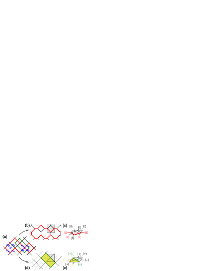
The Toric Code model exhibits $\mathbb{Z}_{2}$ topological order. Its ground state minimizes all Hamiltonian terms individually and can either be seen – cf. Fig. 2a – as an equal-weight superposition of all loop configurations on the original lattice (solid lines) in the $\sigma^{z}$ basis $\{|0\rangle,|1\rangle\}$ (red loops), or of all loop configurations on the dual lattice (dashed lines) in the $\sigma^{x}$ basis $\{|+\rangle,|-\rangle\}$ (green dashed loops). Its ground state has an exact PEPS representation with $D=2$, and a $\mathbb{Z}_{2}$ entanglement symmetry. It can e.g. be derived in the following two inequivalent ways, both relevant for later on: First, shown in Fig. 2bc, by blocking the four sites in every other plaquette to one tensor (gray square), “decorating” the resulting lattice as indicated (without adding physical degrees of freedom on the additional edges), and defining the decorated plaquette as one tensor – that is, the virtual degrees of freedom encode (in the $\{|0\rangle,|1\rangle\}$ basis) whether there is an outgoing loop at that point. Differently speaking, the tensor is constructed such that the virtual index is the difference (equivalently, sum) modulo $2$ of the two adjacent physical indices. Since only closed loops appear, the $\mathbb{Z}_{2}$ entanglement symmetry precisely corresponds to the fact that the number of loops leaving the tensor is even, i.e. there are no broken loops. We denote the generators of the symmetry group as before by $Z$ (here, $Z=\sigma^{z}$). In this representation, inserting a symmetry string corresponds to assigning a $-1$ phase to all loop configurations which encircle the endpoint of the string an odd number of times (a magnetic excitation, or vison), while inserting a non-trivial irrep such as $X_{\alpha}=\left(\begin{smallmatrix}0&1\\ 1&0\end{smallmatrix}\right)$ or $X_{\alpha}=\left(\begin{smallmatrix}0&1\\ 0&0\end{smallmatrix}\right)$ terminates a string and thus gives rise to broken strings (an electric excitation). Following the usual convention, we will denote the anyons by $m\equiv(Z,1)$ and $e\equiv(\mathrm{id},-1)$, with $Z$ the non-trivial group element of $G=\mathbb{Z}_{2}$.

Second, we can work in the dual loop picture (with loops in the $\{|+\rangle,|-\rangle\}$ basis on the dual lattice), Fig. 2d, and assign “color variables” to each plaquette such that loops are boundaries of colored domains. If we choose the same blocking of four sites as before (gray square), we obtain a tensor network representation where the virtual indices carry the color label in the $\{|+\rangle,|-\rangle\}$ basis, and the physical indices correspond to domain walls between colors, that is, the tensor is constructed such that the physical index is the difference modulo $2$ of the adjacent virtual indices (all in the $|\pm\rangle$ basis), Fig. 2e. Here, the $\mathbb{Z}_{2}$ symmetry arises from the fact that flipping all colors leaves the state invariant, and is thus again $Z\equiv\sigma^{z}$. In this dual basis, inserting an irrep $X_{\alpha}$ on a link assigns a relative $-1$ phase to a colored plaquette (i.e. a plaquette enclosed by an odd number of loops in the dual basis), while $Z$ strings flip colors and thus break dual loops.

III.2 Qualitative phase diagram

What is the effect of a magnetic field on the Toric Code model? If we apply only a field $h_{z}>0$ in the $z$ direction ($h_{x}\equiv 0$), the field commutes with the $(\sigma^{z})^{\otimes 4}_{v}$ term, and thus the ground state stays within the closed loop space (on the original lattice). However, the field shifts the balance between different loop configuration towards the vacuum configuration and eventually induces a phase transition into a trivial phase. This disbalance between different loop configurations corresponds to a doping with magnetic excitations, and thus, the phase transition is driven by magnon condensation, while electric excitations become confined. (From now on, the terminology for excitations – electric/magnetic etc. – always refers to this basis, unless explicitly mentioned otherwise.) On the other hand, a pure $x$-field $h_{x}>0$ has the same effect in the dual loop basis but breaks loops in the $\sigma^{z}$ basis, and thus induces a phase transition to a trivial phase through charge condensation. In fact, the whole model (42) has a duality under exchanging $x$ and $z$ and at the same time going to the dual lattice (which also exchanges electric and magnetic excitations), and thus under $h_{x}\leftrightarrow h_{z}$.

Figure 3: Qualitative phase diagram of the Toric Code with $x$ and $z$ magnetic field, Eq. (42). Phase boundaries are indicated in black, and lines which we will study in detail later on in red, labeled by roman numbers I–VII. There is a Toric Code phase (TC) at small field, which for large field transitions into a trivial phase either through flux condensation ($h_{z}>h_{x}$) or charge condensation ($h_{x}>h_{z}$). The model exhibits a duality under exchanging $h_{x}\leftrightarrow h_{z}$ and simultaneously electric and magnetic excitations. Along the self-dual line $h_{x}=h_{z}$, there is a first-order line separating the two different anyon condensation mechanisms through which the trivial phase can be obtained, which ends at a sufficiently large field and is replaced by a crossover regime.

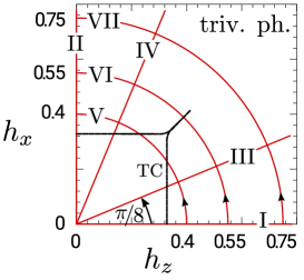
The phase diagram of the model is well known [7, 47, 8, 9, 48] and shown in Fig. 3 (where we mark lines which we are going to study in detail with roman letters I–VII): There is a topological phase at small field which transitions into a trivial phase through either flux condensation (e.g. lines I and III) or charge condensation (lines II and IV), as just discussed. Along the self-dual line $h_{x}=h_{z}$, there is a first-order line which separates the charge condensed from the flux condensed phase (crossed by line VI), which eventually disappears at large enough field, at which point a crossover between the two different ways to obtain the (ultimately identical) trivial phase through anyon condensation appears (line VII). Along the two lines $h_{x}\equiv 0$ (line I) and its dual $h_{z}\equiv 0$ (line II), it is well known that the ground state of the model can be mapped to the ground state of the 2D transverse field Ising model (we discuss the mapping in Sec. III.8 in the context of our order parameters). Generally, the entire transition line between the topological and trivial phase (except along the diagonal) are believed to be in the 3D Ising universality class.

III.3 Variational simulation

For the iPEPS simulation, we work with the $2\times 2$ site unit cell described above (Fig. 2bc) which contains one plaquette. We impose a virtual $\mathbb{Z}_{2}$ symmetry with generator $Z=\openone_{D_{+}}\oplus(-\openone_{D_{-}})$, with $D=D_{+}+D_{-}$ the bond dimension. We optimize the variational energy by iteratively updating the tensor by using Broyden-Fletcher-Goldfarb-Shanno (BFGS) algorithm [49, 50, 51, 52]. After each update, we project the tensor back to the symmetric space. To calculate the gradient of the objective function (i.e. the energy density) with respect to the tensor, we use the corner transfer matrix method [53]. Furthermore, we observe that for the phase transitions between topological and trivial phases, the BFGS algorithm always tends to converge faster and find ground states with lower energies if it is initialized with the tensor that belongs to the topological phase. This observation suggests an important feature of the optimization algorithm: As the algorithm minimizes the energy by updating the local tensor at each step, it is easier to remove than to build up long-range entanglement, and thus, initializing with a state with more complex entanglement order is advantageous.

Figure 4: Variational results for energy (a) and magnetization along the field (b) for the Toric Code with an $x$ field. We find that for $D=4$, the results with symmetry are essentially fully converged; on the other hand, a simulation with $D=2$ with the entanglement symmetries Eq. (4) imposed yields a qualitatively wrong first-order transition For comparison, we also show results obtained without imposing symmetries. See text for further details.

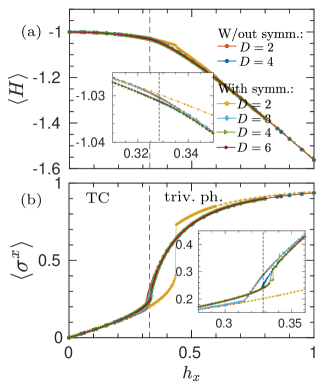
Fig. 4a shows the variational energy obtained for an $x$ field for $D=2,3,4,6$ (where $D=3=1+2=D_{+}+D_{-}$, and otherwise $D_{+}=D_{-}$), with the region around the critical point enlarged in the inset. We find that the optimal variational energy converges rather quickly with $D$, with energies for $D=4$ and $D=6$ already being indistinguishable. In addition, we observe that a symmetric splitting $D_{+}=D_{-}$ is generally favorable. For comparsion, we also show energies obtained by optimizing PEPS tensors without any symmetry. We find that $D=2$ without symmetries is comparable to $D=3$ with symmetries (whereas $D=2$ with symmetries is considerably worse and in fact gives a qualitatively wrong transition, as already observed in Ref. [54]), while $D=4$ with and without symmetry give essentially the same energy. This demonstrates that imposing the symmetry does not significantly restrict the variational space beyond halving the number of parameters, and in particular, it does not necessitate to double the bond dimension due to some non-trivial interplay of constraints. Our findings are also in line with previous observations that for the transverse field Ising model (whose ground state is dual to ours), the energy is essentially fully converged for $D=3$ [55].

In addition, Fig. 4b shows the magnetization along the field. We see that for $D=2$ with symmetries, the phase transition is off and first order. For larger bond dimensions or without symmetries, the point of the phase transitions is however rather close to the exact value. Notably, we see that the ansatz without symmetries undershoots the critical point – that is, it has a tendency towards the trivial phase – while the ansatz with symmetries for $D\geq 4$ slightly overshoots the critical point – that is, it has a tendency to stabilize topological order. Given the connection between entanglement symmetries and topological order, this is indeed plausible. An exception is the case of $D=1+2$ with symmetries, which is closer to the $D=2$ case without symmetries. This indicates that the one-dimensional trivial irrep is still too restrictive, and in this case, the ansatz possibly rather uses the unrestricted degrees of freedom in the $2$-fold degenerate irrep space.

III.4 Topological to trivial transition: Order parameters

Figure 5: Order parameters $\hat{C}_{a}$ for condensation and $K_{a}$ for confinement across the four lines I-IV in Fig. 3, where along lines I and III, magnetic fluxes $a=m$ condense and charges $e$ confine, and vice versa for lines II and IV. Even though I and II, as well as III and IV, are dual to each other, the actual values of the order parameters are different due to the gauge degree of freedom in the construction of electric order parameters – for comparison, the $D=6$ data from the first row is indicated in gray in the dual panels below. Yet, their critical exponents are the same, see Figs. 6 and 7. We also observe that the magnetization of the transverse field Ising model equals $\hat{C}_{m}$ along line I, as proven in Sec. III.8.

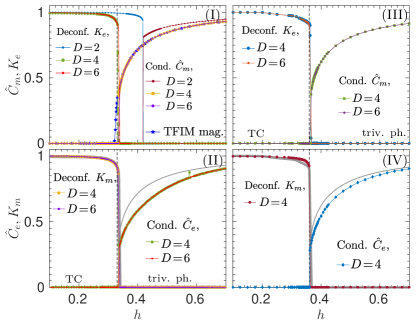
Let us first investigate the behavior of the order parameters as we drive the system from the topological into the trivial phase by increasing the field along a fixed direction. Fig. 5 shows the order parameters for condensation and deconfinement for the four lines I–IV. Here, the first row reports the data for lines I and III, along which fluxes condense, while the second row corresponds to lines II and IV, where charges condense.

Along all four lines, we observe a qualitatively similar behavior: As we increase the field, the deconfinement fraction of the electric (I,III) or magnetic (II,IV) charge decreases and drops to zero rather steeply at the critical point, indicating their confinement. Past the critical point, the condensate fraction for the condensed charge becomes non-zero, with an apparently much smaller slope. We also see that the difference for the data with $D=4$ and $D=6$ is barely visible, confirming what we found for the energy and magnetization in Fig. 4. For line I (top left), we additionally show the data for $D=2$: As already discussed in Section III.3, it does not only give an incorrect critical point, but more importantly also predicts a first- rather than second-order phase transition.

As discussed before, the lines I and II, as well as the lines III and IV (each pair plotted in the same column), are self-dual to each other. On the other hand, they clearly don’t display the same value for the order parameters, as can be seen from the lower panels (lines II and IV), where we have indicated the $D=6$ data for their dual lines I and III as gray lines. This is not surprising – while the pairs of lines are dual to each other, the way in which we extract the order parameters is not; in particular, under the duality mapping the string-like order parameters, which are gauge invariant, get mapped to the irrep-like order parameters, which are not gauge invariant and require a gauge fixing procedure, and vice versa.

This non-uniqueness of the order parameters should not come as a surprise, and is in fact in line with the discussion in Sec. II.4, where we discussed the ambiguities which arise in fixing an order parameter when all we are allowed to use is the symmetry. However, as we have argued there, we expect that for well-designed order parameters (that is, a well-designed gauge fixing procedure), we will observe the same universal signatures, that is, the same critical exponents.

III.5 Topological to trivial transition: Critical exponents

Let us now study the scaling behavior of the order parameters in the vicinity of the critical point.

Figure 6: Scaling of condensate fractions close to the critical point for the lines I-IV. The slope matches the critical exponent $\beta\approx 0.3265$ of the order parameter of the 3D Ising transition.

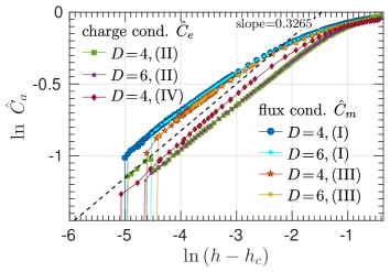
Fig. 6 shows the order parameter for anyon condensation along the four lines I–IV (flux condensation for lines I/III, charge condensation for lines II/IV). We find that all lines show the same critical scaling, which matches the known critical exponent $\beta\approx 0.3265$ of the magnetization in the (2+1)D Ising universality class, consistent with the fact that lines I and II map to the (2+1)D Ising model, and confirming the belief that the whole transition line is in the Ising universality class. Indeed, as we have observed in Fig. 5, the magnetic condensate fraction along line I equals the magnetization in the (2+1)D Ising model, a connection which will be made rigorous in Sec. III.8.

Figure 7: Scaling of deconfinement fractions close to the critical point for the lines I-IV. The slopes along the different lines agree, yet give a critical exponent $\beta^{*}\approx 0.021$, which is not among the known critical exponents of the 3D Ising model. In the text, we discuss interpretations of this exponents in terms of the 2D quantum Ising model, the 3D classical Ising model, and the prefactor of the area law scaling of the Wilson loop in a 3D Ising gauge theory.

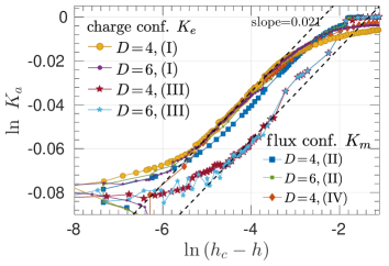
Let us now turn towards the order parameter for deconfinement. Fig. 7 shows the scaling behavior of the order parameter for deconfinement along the same four transitions. We again find that the deconfinement fraction exhibits the same universal scaling behavior along all four lines. However, the critical exponent observed is rather different, and much smaller, namely roughly $\beta^{*}\approx 0.021$. However, the precise value should be taken with care, since (as always) the fitting is rather susceptible to the value chosen for the critical point, and the very small value of $\beta^{*}$ implies a rather large relative error.

What is the nature of this new critical exponent $\beta^{*}\approx 0.021$, which does not even in order of magnitude resemble any known critical exponent of the (2+1)D Ising model? In Sec. III.8, we show that the underlying order parameter maps to an order parameter obtained from a “twist defect line” inserted into the ground state of the (2+1)D Ising model which can be constructed based on its PEPS representation, and which should serve as a disorder operator for the Ising model. This suggests that our technique, developed with the characterization of topological phase transitions in mind, can equally be used to construct novel types of disorder parameters for conventional phases. We construct such a disorder parameter, and study it in detail for the (2+1)D Ising model, in Section IV, where we find that it indeed exhibits the same novel critical exponent $\beta^{*}$. There, we also discuss possible interpretations of this critical exponent, as well as its utility in further characterizing the phase transition.

At the end of this section on critical exponents, let us stress that the fact that our order parameters give the same universal behavior, even though the dual order parameters for the charge and flux condensation transition are constructed in entirely different ways (in particular, charges require gauge fixing, while fluxes don’t) gives an a posteriori confirmation of our approach to extracting order parameters and universal behavior.

III.6 Topological to trivial transition: Anyon masses

Figure 8: Scaling of different correlation lengths along the line II: Inverse mass gap $\xi_{e}$ for charges (in the topological phase), confinement length $\xi^{K}_{m\bar{m}}$ for fluxes (in the trivial phase), and trivial correlation length $\xi_{0}$. The scaling analysis (inset) shows that they all exhibit the same critical exponent, which matches that of the 3D Ising transition.

As discussed, we can also extract length scales from our simulations. Specifically, we can on the one hand extract correlation lengths $\xi_{a}$ for anyon-anyon correlations, or, equivalently, anyon masses $m_{a}=1/\xi_{a}$, for free anyons; a divergence of $\xi_{a}$ (i.e., a closing mass gap) witnesses a condensation of anyon $a$. On the other hand, we can extract a confinement length scale $\xi^{K}_{a\bar{a}}$ for confined anyons, which diverges as the anyons become deconfined.

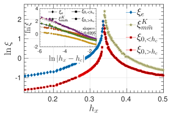
Fig. 8 shows these lengths along the line II, where charges condense. Specifically, we see that the inverse anyon mass of the electric charge, $\xi_{e}$, diverges at the phase transition, while in the trivial phase, the magnetic fluxes become confined, witnessed by a finite confinement length $\xi^{K}_{m\bar{m}}$. In addition, we also show the inverse mass gap for topologically trivial excitations, which diverges at the critical point as well, but is smaller than the other length (typically, one would assume that trivial excitation with the smallest mass gap is constructed from a pair of topological excitations, and thus should have roughly twice their mass, neglecting interactions).

The analysis of the critical scaling of the different lengths reveals that they all display the same scaling behavior, consistent with the critical exponent $\nu$ of the correlation length in the (2+1)D Ising model.

III.7 Rotating the direction of the magnetic field: First-order line and crossover

Figure 9: Behavior for rotating field, lines V–VII, which move between two different condensation mechanisms of realizing the trivial phase. Each column corresponds to one of the lines V–VII. Top row: Condensate and deconfinement fraction of magnetic fluxes. Bottom row: Magnetization $\langle\sigma_{x}\rangle$ and $\langle\sigma_{z}\rangle$, and energy $\langle H\rangle$ (inset). Line V has two second-order phase transitions with a topological phase in between, line VI a first-order phase transition between the two inequivalent trivial phases, and line VII a crossover. For line VII, we rather show the deconfinement fraction, the $x$ magnetization, and the energy for two different choices of initial conditions (following the notation of Ref. [33], $\mathbb{Z}_{1}\boxtimes\mathbb{Z}_{1}$ denotes the flux confined phase and $\mathbb{Z}_{2}\boxtimes\mathbb{Z}_{2}$ the flux condensed phase): We find that while the physical properties converge independent of the initial configuration, the interpretation in terms of a charge or flux condensate becomes unstable around $\phi\approx\pi/4$, indicating a crossover regime where the interpretation of the physical phase in terms of the virtual symmetries breaks down.

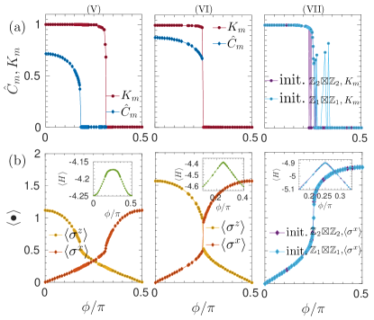
Finally, let us study what happens when we rotate the magnetic field in the $x$-$z$-plane while keeping its strength constant, i.e., moving radially in the phase diagram Fig. 3 along the three lines V, VI, and VII. The resulting data is shown in Fig. 9. Here, the panels in the first line show the condensation and deconfinement fractions for the magnetic particles, while the panels in the second line display the behavior of the $x$ and $z$ magnetization as a function of the angle $\phi$, with the energy shown in the inset. The three columns correspond to the three radial lines V, VI, and VII.

For the line V, we observe two second-order topological phase transitions, first from the trivial to the topological phase through decondensation of the magnetic flux, and subsequently from the topological to the trivial phase through flux confinement. Both $\hat{C}_{m}$ and $K_{m}$ show a clear second-order behavior. Similarly, the two magnetizations $\langle\sigma^{x}\rangle$ and $\langle\sigma^{z}\rangle$ each show a kink, yet again indicative of underlying second-order transitions. On the other hand, the energy does not exhibit clear signs of the phase transitions, which will only show up in its derivatives.

For the line VI, the condensation and the confinement of the magnetic flux coincide at $\phi=\pi/4$: The system undergoes a transition from a flux condensed to a charge condensed (flux confined) phase, without going through an intermediate topological phase. In addition, the order parameters $\hat{C}_{m}$ and $K_{m}$ show a clear jump, indicative of a first-order transition. Similarly, $\langle\sigma^{x}\rangle$ and $\langle\sigma^{z}\rangle$ both exhibit a discontinuity at $\phi=\pi/4$, and the energy shows a kink (and thus a discontinuous derivative).

Finally, along the line VII, the order parameter plot now shows two curves for the deconfinement fraction $K_{m}$, obtained by starting the optimization from two different initial states, either in the charge or in the flux condensed phase. We see that around $\phi\approx\pi/4$, the value of the deconfinement fraction becomes unstable and depends on the choice of the initial phase. This is not all too surprising, since the line VII realizes a crossover between the two different mechanisms of realizing the trivial phase, and in the crossover regime, the interpretation of the trivial phase as an either charge or flux confined phase should become ambiguous; the observed dependence of the deconfinement fraction $K_{m}$ on the initial phase can thus be taken as a fingerprint of this crossover. On the other hand, the lower panel shows that the physical state obtained in the optimization is stable independent of the choice of the initial condition: Both the value of $\langle\sigma^{x}\rangle$ and the energy are independent of the choice of the initial tensor. The observed instability is thus purely a signature of the ambiguous interpretation of the trivial phase in the crossover regime when thought of as a condensed version of the topological model – that is, the way the state is realized on the entanglement level – rather than an instability of the variational method as such.

III.8 Mapping to the (2+1)D Ising model

It is well known that there is an analytical mapping of the ground state of the Toric Code with only an $x$ or a $z$ field to the (2+1)D Ising model (i.e., the 2D transverse field Ising model) [7]. In the following, we will use this mapping to interpret our order parameters for condensation and confinement in terms of conventional and generalized order parameters for the (2+1)D Ising model.

To this end, we start by briefly reviewing the mapping. To start with, consider the Toric Code with a $z$ field,

$$H=-\sum_{p}(\sigma^{x})_{p}^{\otimes 4}-\sum_{v}(\sigma^{z})^{\otimes 4}_{v}-h_{z}\sum_{i}\sigma^{z}_{i}\ .$$ (44)

Since the field $\sigma^{z}_{i}$ commutes with the vertex stabilizers $(\sigma^{z})^{\otimes 4}_{v}$, for any $h_{z}$ the ground state is spanned by closed loop configurations in the $\{|0\rangle,|1\rangle\}$ basis on the original lattice. We can thus work in a dual description of the loop basis, similar to Fig. 2d, but now on the original lattice, where we color plaquettes $p$ with two colors (white=$|0\rangle$, red=$|1\rangle$), and interpret loops as domain walls of color domains, see Fig. 10a. We will label plaquette variables by $|\hat{\imath}_{p}\rangle$ and also mark Hamiltonian terms (Paulis) acting on them by a hat.

Figure 10: Mapping of the Toric Code with field to the Ising model; the mapping works on the space of closed loops. (a) The Ising variables are obtained by assigning color labels $\hat{\imath}$ to the plaquettes, where loops are the domain walls between different colors. (b) $Z$ operators measure the difference between two adjacent colors, $(-1)^{\hat{\imath}_{1}+\hat{\imath}_{2}}$. A magnetic flux ($Z$ string) thus corresponds to a $z$ correlator $(-1)^{\hat{\imath}_{1}+\hat{\imath}_{\ell}}$ between the Ising variables at its ends.

Let us now see how the Hamiltonian (44) acts in the dual basis. The Hamiltonian term $(\sigma^{z})_{v}^{\otimes 4}$ is then trivially satisfied. $(\sigma^{x})_{p}^{\otimes 4}$ flips the loop around $p$, and thus corresponds to flipping the plaquette color $|\hat{\imath}_{p}\rangle$, i.e., it acts as $\hat{\sigma}^{x}_{p}$. On the other hand, the magnetic field $\sigma^{z}_{i}$ assigns a sign $-1$ to a loop on that edge; as loops are domain walls of plaquette colors, this corresponds to $(-1)^{\hat{\imath}_{p}+\hat{\imath}_{p}^{\prime}}$ and thus $\hat{\sigma}^{z}_{p}\hat{\sigma}^{z}_{p^{\prime}}$. In this basis, $H$ (restricted to the loop space, i.e., the ground space of $\sum_{v}(\sigma^{z})_{v}^{\otimes 4}$) thus becomes

$$\hat{H}=-\sum_{p}\hat{\sigma}^{x}_{p}-h_{z}\sum_{\langle p,p^{\prime}\rangle}\hat{\sigma}^{z}_{p}\hat{\sigma}^{z}_{p^{\prime}}\ .$$ (45)

Note again that this is primarily a mapping between the ground states of the models and in particular does not cover excitations beyond the closed loop space.

Let us now see what happens to the anyonic order parameters under this mapping. We will focus our initial discussion on the order parameters constructed from $Z$ strings, since these are gauge invariant and thus yield a unique quantity on the dual Ising model. However, the mapping can also be applied to irrep-like order parameters $X_{\alpha}$, and we will give a brief account of those at the end of the discussion.

First, let us consider the case of a $z$-field as just discussed. In that case, the natural tensor network representation – that is, the one which is constructed from the loop constraint in the $z$ basis – is the one in Fig. 2c. The key property lies in the fact that the irreps on the virtual legs carry the loop constraint (that is, the irrep label of the virtual index equals the sum of the adjacent physical legs in the loop basis). As it turns out, this property is preserved by the variationally optimal wavefunction also at finite field, and thus, anyonic order parameters constructed on the entanglement level still have a natural interpretation in terms of the loop picture, and thus of the dual Ising variables. We have verified numerically that this holds to high accuracy, but it is also plausible analytically: On the one hand, the ground state is constrained to the closed loop space, and on the other hand, the tensor is constrained to the $\mathbb{Z}_{2}$-symmetric space, and thus, identifying these two constraints should give the maximum number of unconstrained variables to optimize the wavefunction.

Now consider the order parameter for condensation, that is, a semi-infinite (or very long finite) $Z$ string, see Fig. 10b. This $Z$ assigns a $-1$ sign to every edge with a loop, and thus for every edge, its effect equals to $(-1)^{\hat{\imath}_{1}+\hat{\imath}_{2}}$ for the two adjacent plaquettes $1$ and $2$, as indicated in Fig. 10b. Thus, for a long string of $Z$’s, the overall action equals $(-1)^{\hat{\imath}_{1}+\hat{\imath}_{2}}(-1)^{\hat{\imath}_{2}+\hat{\imath}_{3}}\cdots(-1)^{\hat{\imath}_{\ell-1}+\hat{\imath}_{\ell}}=(-1)^{\hat{\imath}_{1}+\hat{\imath}_{\ell}}$, and thus the two-point correlator $\hat{\sigma}^{z}_{1}\hat{\sigma}^{z}_{\ell}$ of the Ising model variables. As the condensation order parameter evaluates the overlap of this state with the ground state, it measures $\langle\hat{\sigma}^{z}_{1}\hat{\sigma}^{z}_{\ell}\rangle$: We thus find that the order parameter for flux condensation under a $z$ field maps precisely to the magnetization in the 2D transverse field Ising model – as we have already observed numerically in Fig. 5.

Let us now turn to the case of the $x$ field. Here, the “good” basis is the one spanned by $x$ basis loops on the dual lattice, and thus, we naturally arrive at the tensor network representation Fig. 2e. Its defining feature – which we have again checked numerically to also hold away from the Toric Code point – is that the loops, that is, the physical degrees of freedom in the $\{|+\rangle,|-\rangle\}$ basis, are obtained as the difference of the “color” label of the virtual legs. However, different from before, the color label is not uniquely defined: “Color” corresponds to a decomposition of the bond space as $\mathbb{C}^{D}\simeq\mathcal{S}_{\mathrm{white}}\bigoplus\mathcal{S}_{\mathrm{green}}$, such that $Z$ acts by swapping the two color spaces, $Z\,\mathcal{S}_{\mathrm{white}}=\mathcal{S}_{\mathrm{green}}$. Indeed, by applying any matrix $\Lambda$ which commutes with $Z$, we can obtain another such decomposition (even with a non-orthogonal direct sum). This ambiguity in the choice of the color basis – which becomes precisely the Ising basis after the duality mapping – is a reflection of the fact that in our approach, the only basis fixing comes from the symmetry action, leaving room for ambiguity, as discussed in Section II. However, let us point out that numerically we observe that the “physical index equals difference of colors” constraint is very well preserved for the “virtual $x$ basis”, that is, for the “color projections” $\left(\begin{smallmatrix}\openone&\pm\openone\\ \pm\openone&\openone\end{smallmatrix}\right)$, likely due to the choice of initial conditions (the Toric Code tensor) in the optimization.

Since in this PEPS representation, the Ising degree of freedom in the duality mapping is nothing but the color degree of freedom of the plaquettes, the mapping from the Toric Code to the Ising model can be made very explicit on the level of the PEPS: We need to duplicate the color degree of freedom as a physical degree of freedom, and subsequently remove the original physical degrees of freedom of the Toric Code, similar to an ungauging procedure, see Fig. 11a. The latter can be done, for instance, through a controlled unitary (in the dual basis) controlled by the Ising (color) degrees of freedom, since we know that the physical degrees of freedom are just their differences. Note that for this construction to work, we must know the correct color basis (see above), which however is a property which can be extracted from the tensor (and is only needed in case we want to carry out the mapping explicitly).

Figure 11: (a) Mapping from the PEPS tensor for the Toric Code in a field in the dual representation of Fig. 2e (top) to the Ising model. First, the virtual degrees of freedom (color variables) are copied to physical degrees of freedom, which will become the Ising degrees of freedom (middle; three meeting lines correspond to a delta-tensor in the Ising = $|\pm\rangle$ basis). Then, the physical degrees of freedom of the Toric Code are disentangled, e.g. by using controlled-not operations in the $|\pm\rangle$ basis, controlled by the Ising degrees of freedom (as indicated by the arrows in the middle panel). The disentangled degrees of freedom can then be discarded, resulting in a tensor network for the Ising model (bottom). This can be seen as the reverse of a gauging transformation. (b) Effect of a string of $Z$ operators in the dual representation: $Z$ operators flip the color label of a plaquette, giving rise to a domain wall in the coloring and thus broken dual loops (green line) at the endpoint of the $Z$ string.

For an $x$ field, at the phase transition fluxes become confined. What does the order parameter for flux deconfinement – the normalization of the PEPS with a semi-infinite (or very long) string of $Z$’s placed along a cut – get mapped to in the Ising model? The effect of a $Z$ is to flip the color label. A semi-infinite string of $Z$’s thus flips the color labels along a semi-infinite cut on the lattice. Since the loop variables are the difference of the color variables, and the “closed loop” constraint is implicitly guaranteed by the fact that we arrive at the same color when following a closed curve on the original lattice (recall that the loops live on the dual lattice, and thus the colors on the vertices of the original lattice), flipping the color variable within the plaquette gives rise to a broken “closed loop” constraint for any circle around the endpoint of the $Z$ string – that is, the endpoint of the $Z$ string is the endpoint of a broken loop, see Fig. 11b. Indeed, this is precisely what a magnetic flux corresponds to in the dual basis: a broken string.

However, how can this be mapped to the Ising model? The fact is that it cannot, at least not in a direct way which gives rise to an observable for the Ising model: The mapping to the Ising model precisely relies on the fact that we are in the closed loop space, which is no longer the case in the current basis after introducing a flux. However, we can still give an interpretation of this object in terms of the Ising model, if we describe the ground state of the Ising model in terms of PEPS: After the duality mapping described above, we obtain nothing but a variational PEPS description of the ground state of the Ising model (which becomes exact as the bond dimension grows), constructed from tensors with a $\mathbb{Z}_{2}$ symmetry

(46)

(e.g. by blocking the “ungauged” tensor at the bottom of Fig. 11a with the left and bottom physical index). The order parameter then corresponds to inserting a semi-infinite string of $Z$’s along a cut – a “twist defect” – and computing the normalization of the modified tensor network (relative to the original one). It can be easily seen that this is zero in the ordered phase: In that case, the virtual indices carry the information about the symmetry broken sector, that is, they are all supported predominantly in the same sector, which is flipped by the action of the $Z$ string. Glueing the network with a $Z$ string thus leads to a decrease in normalization which goes down exponentially with the length of the string, as configurations which are approximately in different sectors (with overlap $<1$) are being glued together. Conversely, in the disordered phase we generally expect a non-zero norm, since sufficiently far away from the cut, the spins will be disordered and thus not have a preferred alignment relative to each other along the cut. The only contribution comes from the endpoint of the string (since the spins are still aligned up to a scale on the order of the correlation length). Thus, we expect a non-zero value in the disordered phase and a zero value in the ordered phase (a disorder parameter), and thus a non-trivial behavior as the phase transition is approached.

It is notable that this way, we can define a (dis-)order parameter for the Ising model based on its ground state, even though there is no direct way of measuring it from the ground state itself: Rather, one first has to find a $\mathbb{Z}_{2}$-symmetric PEPS representation of the ground state and construct the order parameter through the effect of twisting the PEPS on the entanglement degrees of freedom. In some sense, it is the combination of the correlation structure of the ground state and the locality notion imposed by the tensor network description on the quantum correlations which makes this possible. This is the reason why the deconfinement order parameter allows us to transgress the mapping to the Ising model, and thus probe properties of the system which are inaccessible when directly probing the system. Let us note that of course, the twisted state is no longer a ground state of the Ising model, and has a large energy around the twist, which however yet again reinforces the point that this type of order parameter is defined through a deformation of the tensor network description of the ground state, and not as a directly observable property of the ground state as such.

This discussion suggests that the same ideas as used in the construction of topological order parameters can also be applied to directly construct disorder operators for phases with conventional order, such as the (2+1)D Ising model; this is studied in detail in Section IV.

Finally, an analogous mapping can be carried out for electric charges. In the case of the $z$ field, a charge breaks a loop, and correspondingly, the duality mapping to the Ising model via plaquette colors breaks down. This can be remedied by introducing a twist along a line emerging from the charge across which the color, that is, the Ising variable, is flipped; this gives rise to precisely the same order parameter constructed from inserting a twist defect in the PEPS representation of the Ising ground state as discussed above. In the case of the $x$ field, on the other hand, the charge operator maps directly to the magnetization operator of the Ising (color) variable, given that it is constructed in the right way relative to the good color basis $\mathcal{S}_{\mathrm{white}}\oplus\mathcal{S}_{\mathrm{green}}$.

IV Entanglement order parameters for conventional phase transitions

The fact that, under the duality mapping between the Toric Code the transverse field Ising model, the deconfinement order parameter gets mapped to a twist defect in the Ising model, which should serve as a disorder parameter, suggests the surprising possibility that tensor networks and the direct access to entanglement which they provide can be used to also construct disorder parameters for conventional phase transitions in entangled quantum matter; and the unexpected critical exponent observed for the deconfinement fraction suggests that this might equally give access to new critical exponents for those conventional transitions.

In the following, we describe a general such framework for the construction of disorder operators for conventional phase transitions, based on the direct access to entanglement provided by tensor networks. We then present numerical results obtained for the (2+1)D transverse field Ising model which confirm that this new kind of disorder operator indeed displays a new critical exponent which is not found otherwise in the 3D Ising theory. We discuss its relation to other disorder operators, and we conclude by explaining how both these disorder parameters and order parameters for conventional phase transitions, as well as the order parameters for topological phase transitions which we constructed, can be understood on a unified footing as entanglement order parameters, that is, order parameters which are constructed to identify (dis)ordering relative to all symmetries of the system – physical as well as entanglement symmetries – on a unified footing.

IV.1 Construction

Consider a Hamiltonian with a global symmetry, $[H(\lambda),U_{g}^{\otimes N}]=0$, where $U_{g}$ is a (faithful) representation of some symmetry group $G$. We will focus on discrete symmetry groups $G$ in the following, though most of our arguments (with some caveats) apply to continuous groups as well. As $\lambda$ changes, the Hamiltonian undergoes a phase transition from a symmetry-broken (ordered) to a symmetric (disordered) phase. As an example, one could e.g. think of the transverse field Ising model or a $\mathbb{Z}_{N}$ Potts or compass model with magnetic fields.

Let us now approximate the ground state (using a variational method) with a tensor network state $|\Psi\rangle$ of some bond dimension $D$, where the symmetry has been encoded in the local tensor $A$,

$$\raisebox{-18.49411pt}{\includegraphics[scale={.9}]{phys-sym-tensor}}\quad.$$ (47)

From the tensor network $|\Psi\rangle$, we can of course compute conventional order parameters, i.e., measure the expectation value of a local physical operator $S$ which does not commute with $U_{g}$, such as an operator $S_{\alpha}$ transforming as a non-trivial one-dimensional irrep $\alpha$ of $G$, $U_{g}S_{\alpha}=\alpha(g)\,S_{\alpha}U_{g}$.

However, from the tensor network for $|\Psi\rangle$ we can also define a disorder parameter as follows: First, define a state $|\Psi_{g}(\ell)\rangle$ by inserting a “twist” with a string of $V_{g}$’s of length $\ell$,

$$|\Psi^{\mathrm{tw}}_{g}(\ell)\rangle=\raisebox{-32.72049pt}{\includegraphics[scale={.9}]{twist-defect}}.$$ (48)

Then, define

$$N_{g}(\ell)=\frac{\langle\Psi^{\mathrm{tw}}_{g}(\ell)|\Psi^{\mathrm{tw}}_{g}(\ell)\rangle}{\langle\Psi(\ell)|\Psi(\ell)\rangle}\ .$$ (49)

What behavior do we expect $N_{g}(\ell)$ to display in the ordered and disordered phase, respectively? To get a qualitative understanding, let us consider the case of $G=\mathbb{Z}_{N}\cong\{0,1,\dots,N-1\}$ with a representation $U_{g}=\sum|g+j\rangle\langle j|$. In the limiting case of a Potts model with zero field, the ground space is spanned by states of the form $\sum w_{j}|j\rangle^{\otimes N}$. The corresponding tensor $A$ (with $V_{g}=U_{g}$) is then a tensor with all indices the same, $A=\sum_{j}w^{\prime}_{j}|j\rangle\langle j,j,j,j|$, with some suitable weight $w_{j}^{\prime}$. This forces all physical and virtual indices in any connected component of the tensor network to have the same value $j$. However, when placing a twist $V_{g}$ ($g\neq 0$) along a cut, $j$ is changed to $g+j$, which is orthogonal to the virtual index on the other side of $V_{g}$, and thus, $N_{g}(\ell)=0$. On the other hand, in the limit of infinite field, the ground state is of the form $|+\rangle^{\otimes N}$, $|+\rangle=\sum|g\rangle$, which can be represented by a tensor $A=|+\rangle\langle t,t,t,t|$, where $|t\rangle$ is a state in the trivial irrep of $V_{g}$. Thus, $V_{g}$ acts trivially on the tensor, and $N_{g}(\ell)=1$.

Figure 12: Order parameter $\langle m_{z}\rangle$ ($z$ magnetization) and disorder parameter $\mathcal{D}$ (response of normalization to inserting a semi-infinite “symmetry twist”) for the (2+1)D transverse field Ising model; see text for details.

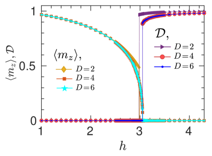
As we interpolate between the two phases, we expect that $N_{g}(\ell)$ interpolates between these two behaviors. In the ordered phase, we expect that the physical degrees of freedom, and thus also the entanglement degrees of freedom, are aligned up to short-ranged fluctuations on the order of the underlying length scale, and thus, we expect $N_{g}(\ell)\sim e^{-\ell/\xi}$, where $\xi$ has a critical exponent $\nu^{*}=\nu$. On the other hand, in the disordered phase, we expect that the spins are not correlated beyond the correlation length, and thus, $N_{g}(\ell)\to\mathcal{D}^{2}>0$. Thus, $\mathcal{D}$ serves as an order parameter for the disordered phase, that is, it is a disorder parameter (also called disorder operator). Note that $\mathcal{D}$ can be considered as the normalization of the ground state tensor network with a semi-infinite twist, given suitable boundary conditions.

IV.2 Numerical results

Let us now study how this disorder parameter behaves for a model with a symmetry breaking phase transition. Specifically, we consider the 2D transverse field Ising model

$$H_{\mathrm{Ising}}=-\sum_{\langle i,j\rangle}\sigma_{i}^{z}\sigma_{j}^{z}-h\sum_{i}\sigma_{i}^{x}\ .$$ (50)

It possesses a $\mathbb{Z}_{2}\equiv\{0,1\}$ symmetry $[H_{\mathrm{Ising}},U_{g}^{\otimes N}]=0$ with $U_{1}=\sigma^{x}$. We variationally optimize a tensor network ansatz for the ground state of $H_{\mathrm{Ising}}$ with a $\mathbb{Z}_{2}$ symmetry encoded,

$$\raisebox{-18.49411pt}{\includegraphics[scale={.9}]{z2-phys-sym-tensor}}\quad,$$ (51)

where $V_{1}=\sigma_{x}\otimes\openone_{D/2}$, using the same numerical methods as described in Section III.3.

Figure 13: Critical scaling for order parameter and disorder parameter at the phase transition. As for the Toric Code, we find that convergence is reached starting from bond dimension $D=4$, while $D=2$ is overly restricted due to the symmetries. (a) For the order parameter $\langle m_{z}\rangle$, we recover the well-known scaling of the 3D Ising unversality class. (b) For the disorder parameter $\mathcal{D}$, we observe a new critical exponent $\beta^{*}\approx 0.024$, which matches the critical exponent observed for the deconfinement fraction in the Toric Code model.

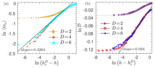
From the optimized tensor, we have determined both the order parameter (the magnetization) and the disorder paramater (the normalization of the twist defect). Fig. 12 shows the results: As expected, we find that in the ordered phase, the order parameter is non-zero and the disorder parameter is zero, and vice versa in the disordered phase. As for the previously considered Toric Code model with magnetic fields, we observe that the disorder parameter vanishes much more steeply as the phase transition is approached. Fig. 13 shows the scaling of the order and disorder parameter as the phase transition is approached. For the order parameter, our data is in agreement with the well-known value $\beta\approx 0.3265$, while for the disorder parameter, we find that it vanishes with a critical exponent of about $\beta^{*}\approx 0.024$, fully compatible with what we observed for the deconfinement fraction in the Toric Code model.

IV.3 Relation to other disorder parameters

Recently, another way of constructing disorder parameters has been proposed, namely to act with a membrane of physical symmetry operators $U_{g}^{\otimes\mathcal{R}}$ on a region $\mathcal{R}$ of the ground state $|\Psi\rangle$, as shown in Fig. 14a, and to compute the overlap with the ground state, i.e., $\Theta:=\langle\Psi|U_{g}^{\otimes M}|\Psi\rangle$. In the ordered phase, this will lead to a state which is approximately orthogonal to $|\Psi\rangle$ locally in all of $\mathcal{R}$, and thus, one expects a volume law scaling $-\log\Theta\sim c\,|\mathcal{R}|$ (here, $|\mathcal{R}|$ is the volume of $\mathcal{R}$). On the other hand, in the disordered phase, acting with $U_{g}^{\otimes\mathcal{R}}$ will only have an effect on the the boundary of $\mathcal{R}$ but not on its (disordered) bulk, and thus we expect a boundary law scaling $-\log\Theta\sim d\,|\partial\mathcal{R}|$ (with $|\partial\mathcal{R}|$ the length of the boundary of $\mathcal{R}$). Specifically, as the phase transition into the ordered phase is approached, $d$ must diverge in order to transition to a volume law scaling, and thus, $d^{-1}$ can serve as an order parameter. Indeed, this is what was observed in Ref. [56] for the transverse field Ising model, and in particular, it was found that $d$ scales as the correlation length $\xi$ and thus, $d^{-1}$ vanishes with the same critical exponent $\nu\approx 0.6205$.

Figure 14: Disorder parameter constructed from a physical symmetry action on a membrane (panel a) and its reformulation in terms of an entanglement symmetry (panel b), see text for details.

It is remarkable that these two different ways to define disorder parameters result in such different scaling behaviors. Are these two order parameters entirely unrelated? To start with, note that if a tensor network with symmetric tensors is used, it is immediate that a physical membrane $U_{g}^{\otimes\mathcal{R}}$ is equivalent to a virtual loop operator $V_{g}^{\otimes\partial\mathcal{R}}$ as shown in Fig. 14b. Thus, $e^{d}$ can be interpreted as the overlap per unit length of the tensor network with and without an infinite (not: semi-infinite!) twist line. We thus see that both order parameters share quite some similarity: They are both obtained by measuring the effect of inserting twist defects in the tensor network. However, they are also rather distinct in other ways: While our disorder parameter is obtained from an open-ended string, the other is obtained from a closed or infinite string. Moreover, in one case the order parameter is a normalization, while in the other, it is an overlap. And finally, one of them has a length-dependent contribution and needs to be taken per unit length, while the other one doesn’t display such a behavior (that is, it is length-independent), an distinction clearly confirmed by the numerics.

It is nevertheless tempting to think that the two order parameters should, in fact, behave the same way, by using a Wick rotation argument. The pronounced difference observed between these two order parameters in the numerical simulations, however, makes it clear that this is not the case. Let us nevertheless briefly discuss the Wick rotation argument, and also why one shouldn’t expect such a behavior. Specifically, we can think of the ground state of a Hamiltonian as being obtained from imaginary time evolution $e^{-\beta H}$ of an arbitrary initial state; through trotterization, one arrives at a 3D tensor network for the ground state as well as expectation values, which can at the same time be seen as a way to construct the 2D tensor network by blocking columns. Specifically, for the Ising model, one obtains a classical 3D Ising partition function in the limit of extreme anisotropy, namely couplings $2\beta J_{\parallel}=-\log(\epsilon h)\gg 1$ along the imaginary time direction and $2\beta J_{\perp}=\log((1+\epsilon)/(1-\epsilon))\ll 1$ along the spatial directions, where the limit $\epsilon\to 0$ needs to be taken. The two order parameters can now both be understood as inserting a twist (i.e., coupling spins antiferromagnetically) along a half-infinite plane. For our disorder parameter, the boundary line of this plane is aligned along the imaginary time axis, while for the one of Ref. [56], it is alinged along a spatial axis. Given the extreme anisotropy limit which needs to be considered, it is indeed plausible that these two disorder operators would exhibit different scaling behavior, as is clearly confirmed by the numerics.

IV.4 What could $\beta^{*}$ be?

A possible hypothesis for the value of $\beta^{*}$ in terms of the underlying CFT could be based on assuming an effective description at the critical point where physical and virtual degrees of freedom in the PEPS behave in the same way and thus exhibit the same scaling of their correlations with an exponent $1+\eta$ (with $\eta$ the anomalous dimension). Re-glueing the spins after twisting and integrating over a finite cut suggests an exponent $\eta$ for a twist line correlator at the critical point, and thus a critical exponent $\beta^{*}=\eta\nu/2$ for the order parameter away from criticality (where $\beta=(1+\eta)\nu/2$); the resulting value $\beta^{*}\approx 0.0114$ for the 3D Ising model agrees reasonably with the magnitude of the observed value, given the difficulty to extract critical exponents with high absolute precision. Indeed, this speculative formula also matches the results obtained for topological phase transitions observed in PEPS families which map to the (2+0)D Ising model [25], as well as the (2+0)D Ising model itself (where $\beta=\beta^{*}=1/8$ due to the self-duality of the model) and mean field (where $\beta^{*}=0$).

Could the critical exponent $\beta^{*}$ give us access to new universal signatures of the phase transition? First off, this depends on whether $\beta^{*}$ can be derived from the underlying CFT at criticality, or more generally the scaling exponents of the model at criticality. While this is certainly plausible, the construction through twisting the PEPS ground state – which takes us outside the ground space! – nevertheless leaves the possibility that the critical exponent can, in fact, only be obtained from the exponents of some extension of the model. In case $\beta^{*}$ can be derived from the scaling dimensions at criticality, it will not give access to new information for the (2+1)D Ising model, since the model if fully specified by two scaling dimensions (which can be computed from $\beta$ and $\nu$). On the other hand, this need no longer be true for more complex models with more scaling dimensions, in which case case $\beta^{*}$ might give access to additional universal data. Finally, even in case that the formula conjectured above holds, or otherwise $\beta^{*}$ could be computed from $\beta$ and $\nu$, the exponent $\beta^{*}$ of the disorder operator still provides an additional probe for universal behavior which, depending on the concrete values of the exponents in a given scenario, might well allow to obtain higher accuracy data about scaling dimensions as compared to other exponents.

IV.5 Entanglement order parameters: A unifying perspective

Let us conclude this section by explaining how topological order parameters and the disorder parameters obtained from “entanglement twists” can be understood on a unified footing as the most general order parameters for tensor networks with symmetries. To this end, consider a tensor with symmetry

(52)

where now, $U_{g}$ is not necessarily a faithful representation – therefore, this does, in particular, include the case of topological order (for $U_{g}=\openone$), phases with physical symmetries exhibiting conventional order ($U_{g}$ faithful), as well as symmetry enriched (SET) phases.

The most general order parameter for a tensor network with such a symmetry should be an object which detects the breaking of any of those of the symmetries, that is, an operator on either the physical or the entanglement degrees of freedom which transforms as an irrep of the symmetry group. However, placing such an irrep $S_{\alpha}$ on the physical level can always be replaced by placing a corresponding irrep $R_{\alpha}$ on the virtual level, as

 and  (53)

transform in the same way. We thus find that the most general order parameter is given by irreps acting on the ket and/or bra virtual indices which transform as an irrep of the joint ket+bra symmetry group (depending on the representation $U_{g}$, this can be $G$ (conventional order), $G\times G$ (topological order), or something in between, as the physical symmetry action has to cancel when building the ket-bra object). Similarly, disorder operators can be constructed by strings of $V_{g}$ on the entanglement or by membranes of $U_{g}$ on the physical degrees of freedom. However, yet again, due to the relation shown in Fig. 14, any physical symmetry membrane can be replaced by a string of $V_{g}$ on the virtual layer. We thus find that the most general disorder parameter is constructed from symmetry strings on the ket and/or bra layer of the entanglement. As for the case of topological order parameters, order and disorder parameters can be conbined, such as to detect symmetry protected order (the most prominent example being string order parameters for 1D symmetry protected phases).

We thus find that in all those cases, it is sufficient to construct order/disorder parameters right away on the level of the entanglement degrees of freedom, that is, as entanglement order parameters. From this perspective, the order parameters for topological and for conventional order, including the new disorder parameter, are just different manifestations of entanglement order parameters in settings with different symmetry realization.

V Discussion

Before concluding, let us discuss a few relevant aspects with regard to our method.

V.1 Gauge fixing

First, an interesting question is linked to the gauge fixing involved in our algorithm. It can be easily checked that applying a random gauge of the form (3) independently for each point in the phase diagram leads to a completely random and uncontrolled behavior of the order parameter. Applying the gauge fixing procedure after such a scrambling always returns the same tensor and thus stabilizes the behavior of the order parameter again. On the other hand, the data obtained in numerical simulations typically does not display a random gauge; rather, we expect the gauge to be determined by the choice of the initial tensor and the way in which the optimization is performed (though this can of course involve randomness or other effects which destabilize the gauge). In particular, we have found that for data which has been obtained by independently optimizing the tensor for the individual points in the phase diagram, the optimized tensors yield an order parameter with noticable residual noise, which can be significantly improved by applying the gauge fixing procedure. On the other hand, we have also found that in order to obtain the best data, it is advisable to initialize the tensors with the optimal tensors obtained for a nearby point in the phase diagram (i.e., to adiabatically change the field); in that case, we observe that the order parameters obtained from the optimized tensors already display a very smooth behavior, and applying an additional gauge fixing step only leads to minor improvements. This is certainly plausible, given that an adiabatic change of the field only leads to minor changes in the tensor and thus ideally to no significant drift in the gauge.

We have also compared different gauge fixing schemes (in particular, the one described in Sec. II.5, and a “symmetric” gauge fixing where the spectrum of the left and right fixed point in Eq. (26) are fixed to be equal), and found that they lead to slightly different order parameters, which however display identical critical exponents, as expected.

V.2 Endpoints and vacua

Second, the construction of our order parameters leaves open degrees of freedom in the endpoint operators. On the one hand, in case of a trivial irrep label, $\alpha=1$, there is no reason to restrict the endpoint to a single irrep block $\gamma$ – recall that we made this choice to obtain gauge-invariant quantities when considering pairs of particle-antiparticle endpoints – since the gauge already cancels out for each endpoint individually. We can thus replace $X_{\alpha,\gamma}$ in Eqs. (31) and (33) by any object in the trivial irrep sector, that is, any $r=\sum w_{\gamma}X_{\alpha=1,\gamma}$ (differently speaking, any $r$ with $V_{g}rV_{g}^{\dagger}=r$). We have investigated this degree of freedom and found that while it affects the (non-universal) value of the order parameter, it does not affect the universal scaling behavior.

In addition, the endpoint operators $X_{\alpha,\gamma}=\delta_{\gamma+\alpha,\gamma}\otimes M_{\alpha,\gamma}$ defined in Eq. (23) leave the freedom of choosing different $M_{\alpha,\gamma}$ in the degeneracy space of the irreps. Choosing different such $M_{\alpha,\gamma}$ can affect the stability of the resulting curve (making a fitting of the scaling difficult), where we have observed that our choice $M_{\alpha,\gamma}=\openone$ leads to a particularly stable behavior. A considerably more stable way of choosing $M_{\alpha,\gamma}$ different from $\openone$ is to impose that $M_{\bar{\alpha},-\gamma}=M_{\alpha,\gamma}^{-1}$, motivated by the fact that this is the way how these two blocks transform relative to each other under gauge transformations. Indeed, this yields more stable order parameters (again with different values but the same scaling behavior), but depending on the choice of $M$, we still observe cases where the curve becomes unstable and does no longer allow for a reliable scaling analysis. This suggests that the chosen gauge fixing is special, and changing the gauge by a fixed invertible matrix can decrease the stability of the method.

On the other hand, one might wonder whether one can also replace the vacuum $X_{\mathrm{vac}}=\openone$ in Eqs. (31-33) by a different operator describing an excitation in the trivial sector. We found that this is not the case, as it can affect the observed critical behavior. This might be understood as follows: An excitation in the trivial sector can be seen as a particle-antiparticle pair; since each of those displays critical behavior at the phase transition, we also expect – and observe – such a non-analytical behavior for order-parameter-like quantities for those trivial particles. While these are not proper order parameters – that is, they are non-zero on both sides of the transition – they nevertheless display a non-analyticity at the phase transition (similar to the magnetization, cf. Fig. 9). Thus, dividing the order parameters by such a non-analytic normalization in Eqs. (34) and (35) will affect the critical behavior in the regime where its non-analyticity dominates its non-zero value, and thus potentially mask the true critical scaling. We thus conclude that for the normalization, one should use the trivial vacuum $X_{\mathrm{vac}}=\openone$.

V.3 Why does it work at all?

An interesting question one might raise is why the method works at all, and why it gives meaningful results also in the trivial phase.

In particular, one might argue that if the PEPS optimization is carried out with a very large bond dimension $D\to\infty$, one can easily transform any iPEPS into one which additionally carries the entanglement symmetry (4), yet without coupling this entanglement symmetry to the physics of the system at all: To this end, simply take any PEPS with bond dimension $D$, and construct a new PEPS with $D^{\prime}=2D$ by tensoring each virtual index with a qubit which is placed in the $|0\rangle$ state. The new tensor has a $\mathbb{Z}_{2}$ symmetry under the action of $\openone\otimes\sigma^{z}$, while at the same time, the additional virtual degree of freedom is completely detached from the original PEPS, and thus can by no means give any information whatsoever about the physics of the system.

The answer is that the finiteness of the bond dimension is relevant here – as long as the bond dimension is finite, using all degrees of freedom is variationally favorable; in particular, it is favorable for the method to use the symmetry-constrained degrees of freedom to encode the topological degrees of freedom, as we have seen. In that sense, going to a large bond dimension – where no energy is gained from the extra bond dimension within numerical accuracy – could in principle destabilize the method, likely around a bond dimension $|G|D_{\mathrm{crit}}$, where $D_{\mathrm{crit}}$ is the dimension where no further energy is gained in an unconstrained optimization. (E.g., for the 2D Ising model, it has been found that beyond $D_{\mathrm{crit}}=3$, variational optimization does not work reliably any more due to the marginal gain in energy [55]; it is thus natural to expect for the Toric Code $D_{\mathrm{crit}}=6$).

A related question is why the method still gives useful information in the trivial phase, given that it probes the properties of topological excitations. This should, however, not come as a surprise: A phase transition into an ordered phase (either conventionally, i.e., magnetically, or topologically ordered) is characterized by the formation of ordered domains of increasing size $\xi$ which diverges at the phase transition. Thus, the structure of the ordered phase is already present in the disordered phase sufficiently close to the transition, and thus, using the entanglement symmetries to store this information is yet again advantageous. On the other hand, we have also seen in Fig. 9 that for very large fields, where the corresponding length scale becomes very small, and only a very small bond dimension is needed for an accurate description of the ground state, the data extracted from the entanglement degrees of freedom indeed starts to become unstable and sensitive to initial conditions, with no effect on the physical properties of the variational state, that is, it no longer provides meaningful information about the system.

V.4 Where does the additional order parameter come from?

We have seen that in the Toric Code model, we were able to use our method to construct an additional order parameter, which does not show up in the (2+1)D Ising model. This might come as a surprise, since there exists a mapping from the ground state of the Toric Code model to that of the (2+1)D Ising model. How can this be the case?

The explanation lies in the fact that by being constructed on the entanglement degrees of freedom of the optimized ground state tensor, our order parameters can leave the ground space of the Toric Code, and thus the mapping to the ground space of the Ising model breaks down. This has been discussed in Sec. III.8: Inserting string operators at the entanglement level breaks loops, and the mapping to the Ising model only works within the closed loop space.

As we have seen subsequently in Section IV, this also opens up a new avenue for constructing order parameters based on PEPS which is not restricted to topological order, by encoding physical symmetries locally in the iPEPS tensor, and computing the response of the wavefunction (i.e., the change in normalization) to the insertion of a symmetry string along a cut at the entanglement level. Such a “disorder operator” will show a distinct behavior in the two phases: In the ordered phase, where all degrees of freedom are aligned, it will give rise to misaligned degrees of freedom all along the cut, and thus to a norm zero. On the other hand, in the disordered phase, the spins (and thus tensors) are only correlated at the scale of the correlation length: The misalignment along the cut will thus only persist for that distance, and thus, a finite value of the order parameter is expected.

In some sense, the ability of these order and disorder parameters to probe otherwise unaccessible properties can be understood as emerging from the interplay between the symmetry and entanglement structure of the wavefunction with the local description enforced through the PEPS description: This local description exposes the way in which symmetries and entanglement build up locally, and thereby gives access to information which cannot be simply extracted through local or string-like operators acting on the physical degrees of freedom, as those don’t give access to information about how the quantum correlations in the system organize locally.

In summary, PEPS with symmetries form a framework which allows to access additional order parameters also for conventional phases, by optimizing the iPEPS tensor and subsequently studying the response to symmetry twists inserted on the entanglement level. They thus allow to extend disorder parameters – previously only defined for classical models at finite temperature [57, 58] – to the domain of quantum phase transitions.

VI Conclusions

In conclusion, we have presented a framework to construct and measure order parameters for topologically ordered phases. Our framework is based on variational iPEPS simulations with a fixed entanglement symmetry, and the ability of these symmetries to capture the behavior of anyons, and in particular their disappearance at a phase transition through anyon condensation and confinement. Importantly, we have devised methods to construct and measure these order parameters in a gauge invariant way, making the method suitable for fully variational iPEPS simulations where nothing but the symmetry is imposed.

We have applied our framework to the study of the Toric Code model in simultaneous $x$ and $z$ fields, and have found critical exponents for condensation $\beta$ and for the length scales associated with the mass gap and confinement, $\nu$, which are consistent with the 3D Ising universality class for the entire transition. In addition, however, our method also allowed us to unveil a novel critical exponent for the order parameter measuring the deconfinement fraction. This demonstrates the suitability of our framework for the microscopic study of topological phase transitions.

We have then argued that our approach can, in fact, be understood more generally as a way of defining order parameters using all symmetries present in the iPEPS tensors, leading to a general framework of entanglement order parameters, treating topological order and global physical symmetries on a unified footing. In particular, we have demonstrated that this allows to define novel disorder operators for conventionally ordered phases such as the (2+1)D Ising model. We have numerically studied the behavior of the disorder parameter for the latter model at criticality, and found that it exhibits the same unknown critical exponent as for the Toric Code above, demonstrating the power of the PEPS framework and entanglement order parameters to probe critical behavior in novel ways.