Smaller11 $\BODY$ Smaller08 $\BODY$ MnLargeSymbols’164 MnLargeSymbols’171

^a Department of Physics & Astronomy, University of California,

Riverside, CA 92521

^b ICTP South American Institute for Fundamental Research & IFT-UNESP,

R. Dr. Bento Teobaldo Ferraz 271, São Paulo, Brazil

Abstract

We investigate how quantum dynamics affects the propagation of a scalar field in Lorentzian AdS. We work in momentum space, in which the propagator admits two spectral representations (denoted “conformal” and “momentum”) in addition to a closed-form one, and all have a simple split structure. Focusing on scalar bubbles, we compute the imaginary part of the self-energy ${\rm Im}\Pi$ in the three representations, which involves the evaluation of seemingly very different objects. We explicitly prove their equivalence in any dimension, and derive some elementary and asymptotic properties of ${\rm Im}\Pi$.

Using a WKB-like approach in the timelike region, we evaluate the propagator dressed with the imaginary part of the self-energy. We find that the dressing from loops exponentially dampens the propagator when one of the endpoints is in the IR region, rendering this region opaque to propagation. This suppression may have implications for field-theoretical model-building in AdS. We argue that in the effective theory (EFT) paradigm, opacity of the IR region induced by higher dimensional operators censors the region of EFT breakdown. This confirms earlier expectations from the literature. Specializing to AdS₅, we determine a universal contribution to opacity from gravity.

Introduction

In Lorentzian flat space, propagators of perturbative quantum field theory are proportional to

$$\frac{i}{p^{2}-m^{2}+\Pi(p)}\,.$$ (1)

$\Pi$ is the self-energy, i.e. the bilinear operator arising from quantum loops. This self-energy dresses the free propagator, yielding a Born series which sums to Eq. (1). Unitarity cuts relate the imaginary part of $\Pi$ to processes ending into asymptotic states. ${\rm Im}\Pi$ resolves singularities occurring in the timelike region $p^{2}>0$, making leading loop effects an unavoidable ingredient of QFT in the timelike region.

In Lorentzian Anti-de Sitter (AdS) space—as in any other background—the propagator is also dressed by self-energy insertions, as pictured in Fig. 1. How does this dressed propagator behave in AdS? Some limited intuition from flat space might be used (see Sec. 1.1), but in any case an explicit, quantitative description of the effects of quantum dressing remains to be obtained. In this work we set out to investigate some of these effects.

Unlike in flat space, AdS lacks asymptotic states to define a standard $S$-matrix, and thus a standard optical theorem Balasubramanian:1999ri ; Giddings:1999qu . Interestingly, it was recently discovered that an AdS unitarity cut in a certain spectral representation plays the role of halving diagrams Meltzer:2019nbs . In our study we will note the interplay between this AdS cut and the imaginary part of the self-energy.

A study of the dressed propagator involves evaluating loops in AdS and summing the Born series. But propagators in position space are complicated functions of the AdS geodesic distance, making every step a challenging calculation. Loops in AdS have been an intense topic of study, see Heemskerk:2009pn ; Penedones:2010ue ; Cornalba:2007zb ; Fitzpatrick:2011hu ; Alday:2017xua ; Alday:2017vkk ; Alday:2018pdi ; Alday:2018kkw ; Meltzer:2018tnm ; Ponomarev:2019ltz ; Shyani:2019wed ; Alday:2019qrf ; Alday:2019nin ; Meltzer:2019pyl ; Aprile:2017bgs ; Aprile:2017xsp ; Aprile:2017qoy ; Giombi:2017hpr ; Cardona:2017tsw ; Aharony:2016dwx ; Yuan:2017vgp ; Yuan:2018qva ; Bertan:2018afl ; Bertan:2018khc ; Liu:2018jhs ; Carmi:2018qzm ; Aprile:2018efk ; Ghosh:2018bgd ; Mazac:2018ycv ; Beccaria:2019stp ; Chester:2019pvm ; Beccaria:2019dju ; Carmi:2019ocp ; Aprile:2019rep ; Fichet:2019hkg ; Drummond:2019hel ; Albayrak:2020isk ; Albayrak:2020bso ; Meltzer:2020qbr . AdS loops are often evaluated in position space and are given by fairly complex expressions. A summation of the Born series in the spectral formalism in the $O(N)$ model can be found in Carmi:2018qzm . However the expressions involve spectral integrals and are fairly difficult to handle for further analysis.

We choose to investigate the dressed propagator by working in the position-momentum space derived from Poincaré coordinates $(p^{\mu},z)$. Though some symmetry is lost when going in this Poincaré position-momentum space, various representations of the propagator become simultaneously available which take a simple form. Momentum space is also the natural language to study the loop summation and to connect with flat space QFT knowledge and tools. Among the above references, Albayrak:2020isk ; Albayrak:2020bso and Meltzer:2020qbr involve calculations in momentum space—the use of momentum space proves to be instrumental in these works. Momentum space has also been used in diverse studies of tree-level amplitudes Raju:2010by ; Raju:2012zs ; Raju:2012zr ; Raju:2011mp ; Bzowski:2013sza ; Bzowski:2015pba ; Bzowski:2018fql ; Bzowski:2015yxv ; Isono:2019ihz ; Isono:2018rrb ; Isono:2019wex ; Coriano:2018bbe ; Coriano:2019dyc ; Maglio:2019grh ; Gillioz:2018mto ; Coriano:2013jba ; Bzowski:2019kwd ; Gillioz:2019lgs ; Farrow:2018yni ; Nagaraj:2019zmk ; Albayrak:2018tam ; Albayrak:2019yve ; Albayrak:2019asr and in the calculation of cosmological observables Maldacena:2002vr ; Maldacena:2011nz ; Mata:2012bx ; Kundu:2014gxa ; Ghosh:2014kba ; Arkani-Hamed:2015bza ; Kundu:2015xta ; Sleight:2019mgd ; Sleight:2019hfp ; Sleight:2020obc ; Arkani-Hamed:2017fdk ; Arkani-Hamed:2018bjr ; Benincasa:2018ssx ; Benincasa:2019vqr ; Arkani-Hamed:2018kmz ; Baumann:2019oyu ; Baumann:2020dch .

When considering the effective field theory (EFT) of gravity, the theory necessarily becomes strongly coupled in the IR region of the Poincaré patch. This feature was pointed out at a qualitative level in ArkaniHamed:2000ds , wherein it was suspected that rapid oscillations of the timelike propagator may render this region inaccessible, hence censoring superPlanckian effects. A more accurate analysis involving dressed propagators in the timelike region of AdS has been initiated in Fichet:2019hkg and Costantino:2020msc . The present work also serves to reinforce and complete these EFT-oriented analyses.

Why might one study quantum field theory in anti-de Sitter space in the first place? AdS is a maximally symmetric background, it is a laboratory to understand QFT in more general curved spacetime. In AdS the negative curvature regulates infrared divergences, which can teach us about flat space QFTs Callan:1989em . The AdS metric is conformally flat, such that boundary conformal theories in flat space can be studied by placing a CFT in the AdS bulk McAvity:1995zd ; Giombi:2020rmc . But, perhaps more importantly, AdS turns out to be a unique window into strongly coupled gauge theories and into quantum gravity as a consequence of the AdS/CFT correspondence (for initial works see Maldacena:1997re ; Gubser:1998bc ; Witten:1998qj ; Freedman:1998bj ; Liu:1998ty ; Freedman:1998tz ; DHoker:1999mqo ; DHoker:1999kzh , for some reviews see Aharony:1999ti ; Zaffaroni:2000vh ; Nastase:2007kj ; Kap:lecture ), which identifies a dual conformal field theory (CFT) living on the boundary of AdS. QFT in AdS is also interesting for phenomenological reasons. Models in AdS can solve the electroweak hierarchy problem Randall:1999ee , give rise to braneworlds with reasonable modifications to 4d gravity Randall:1999vf ; Brax:2003fv , and model strongly coupled dark sectors vonHarling:2012sz ; McDonald:2010fe ; McDonald:2010iq ; Brax:2019koq .

Preliminary Observations

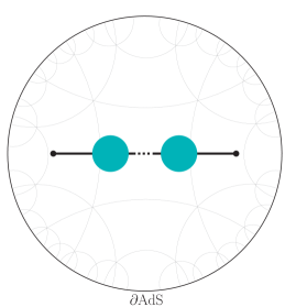
Figure 1: A propagator dressed by generic self-energy insertions in the bulk of AdS.

The principal question we want to answer is: How does quantum dynamics affect the propagation of a field in AdS spacetime? Here we lay down preliminary observations to set the stage and sharpen the scope of our study.

Our interest is in interacting field theories. Our notion of field here includes matter fields as well as gravity—treated as an EFT in the sub-Planckian regime. For the propagating field itself, we restrict our study to a scalar. We will study quantum effects induced both from matter interactions and from gravity on this propagating scalar.

The presence of interactions results in a non-trivial self-energy operator $\Pi$ dressing the propagating field. One representation of a dressed propagator is as a Born series—a term of the series is pictured in Fig. 1. Another representation of dressing is via the equation of motion following from the quantum effective action, schematically

$$\sqrt{|\gamma|}{\cal D}\,G-G*\Pi=-i\delta\,.$$ (2)

Here ${\cal D}$ is the differential operator giving rise to the free equation of motion, $\gamma$ the background metric on which the field propagates, $\delta$ a Dirac delta and $G$ is the propagator. A perturbative treatment of the self-energy operator in Eq. (2) generates the Born series representation.

The qualitative differences in field propagation between the free and interacting theories are expected to occur most clearly in the timelike region of spacetime. This feature is not specific to AdS. It is expected simply because in the timelike regime, the self-energy tends to develop singularities and become complex-valued. In particular, while the solutions of the free homogeneous EOM would tend to be oscillating, in the interacting theory $\Pi$ can develop an imaginary component which introduces an exponential behaviour in the solutions. This then translates as an exponential damping in the Feynman propagator described in Eq. (2), where the effect comes from ${\rm Im}\Pi$. These rough considerations only rely on the analytical structure of $\Pi$, not on the existence of asymptotic states, hence they are valid for QFT in curved spacetime.

The damping effect can be seen in Lorentzian flat space—though the position space propagator behaves as a power law in the free theory, it exponentially decays in the interacting theory. Assuming a constant imaginary part ${\rm Im}\Pi\equiv m\Gamma$ in Eq. (1) gives rise to a propagator decaying as

$$G(X,X^{\prime})\sim\frac{m^{\frac{d}{2}-1}}{(\Delta X)^{\frac{d}{2}}}e^{-\frac{\Gamma\,\Delta X}{2}}$$ (3)

in $d+1-$dimensions, with $\Delta X=\sqrt{\eta_{MN}X^{M}X^{\prime N}}\in\mathbb{R}$ a timelike interval. The free theory behaviour amounts to having $\Gamma=0$ in Eq. (3): there is no exponential decay in this case. This exponential suppression means that particles with $\text{Im}\Pi\neq 0$ decay through time. This interpretation cannot be used in curved spacetimes, where intuitions using asymptotic states are not necessarily valid.

The above points indicate that the imaginary part of the self-energy, ${\rm Im}\Pi$, is likely to play an important role in the field propagation in AdS. Consequently ${\rm Im}\Pi$ will be a central object in our study.

In flat space, ${\rm Im}\Pi$ implements unitarity cuts. This is not necessarily true in AdS since there are no asymptotic states and hence no standard optical theorem. However an AdS cut operation has been introduced in Meltzer:2019nbs —and a corresponding operation has been identified in the dual conformal theory Caron-Huot:2017vep . In the scope of the present work, we will note the interplay between the ${\rm Im}()$ and the AdS cut operations. We do not delve into the CFT side apart from using some elementary results.

At leading order in the loop expansion, ${\rm Im}\Pi$ is expected to be finite in any spacetime dimension. This is because the divergences renormalize local bilinear operators, which contribute to the real part of $\Pi$. The mass term in $\cal D$ may for instance be renormalized. We focus on a finite part of $\Pi$ hence renormalization aspects do not require further discussion and can be ignored.

Summary of Results

Working in Poincaré position-momentum space (i.e. in Fourier-transformed Poincaré coordinates), three representations of the propagator become simultaneously available and take simple forms: a closed-form “canonical” representation, a conformal spectral representation, and a momentum spectral representation. Each of these representations is useful to illuminate different properties of the AdS loop.

We consider cubic couplings, such that the self-energies considered always have a bubble topology. We obtain the following results.

• We derive the imaginary part of the simplest scalar bubble in the three representations mentioned above. In the conformal spectral representation, AdS/CFT arises and we recover various results from the literature.  We prove the equivalence of all three representations of $\text{Im}\Pi$ and show some of its elementary and asymptotic properties.

• We solve the dressed equation of motion for timelike momentum $p^{2}>0$ in the conformally flat region $pz\gg 1$ using a WKB-type approximation. We work in the momentum spectral representation of ${\rm Im}\,\Pi$ and the canonical representation of the propagator. To render the calculations analytically tractable and obtain a closed-form result, we employ kinematic and saddle-point approximations. This is a new method of studying the dressed propagator.

• The dressing induces an exponential damping of the propagator in the $pz\gg 1$ region. This damping behaviour occurs even if a single point is in the conformally flat region, i.e. $pz_{<}\ll 1$, $pz_{>}\gg 1$, which includes the boundary-to-bulk propagator with $pz\gg 1$ as a particular case. This regime has no flat-space equivalent—the $pz\ll 1$ region vanishes if one Weyl-transforms to flat space. Renormalizable interactions may not give rise to an exponential damping, but operators of sufficiently high dimension—as present in an EFT—will induce it. This is pictured in Fig. 2.

• In the EFT paradigm, the EFT breaks down when higher dimensional operators give contributions of the same order. In AdS this occurs at sufficiently large $pz$, i.e. in the IR region of the Poincaré patch. Working in the EFT paradigm, we find that the exponential damping censors the region of EFT breakdown.

• In case of a scalar field theory in AdS₅, the leading damping occurs from the $\Phi^{3}-\Phi\partial_{M}\Phi\partial^{M}\Phi$ bubble. The timelike propagator behaves schematically as

  $$G(p;z,z^{\prime})\propto e^{-c\frac{k}{\Lambda}(pz_{>})^{2}}\,$$ (4)

  where the coefficient $c=O(10^{-2})$ (see Sec. 5.4) includes suppression by a loop factor and estimates from 5D dimensional analysis. Here $k$ is the AdS curvature and $\Lambda$ characterizes the strength of couplings in the EFT.

• A partial contribution from bulk gravity in AdS₅ leads to the suppression

  $$G(p;z,z^{\prime})\propto e^{-c^{\prime}\kappa^{2}(pz_{>})^{4}}\,$$ (5)

  with $c^{\prime}=O(10^{-6})$ and $\kappa=\frac{k}{M_{\rm Pl}}$. This effect depends only on the strength of gravity $\kappa$.

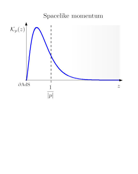
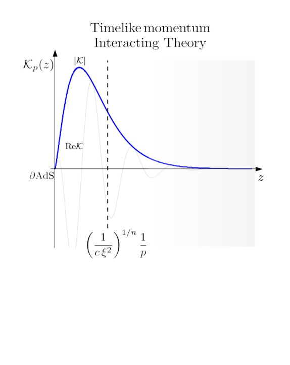
Figure 2: AdS boundary-to-bulk propagators in Poincaré position-momentum space $(p^{\mu},z)$. For spacelike momentum the propagator decays exponentially for $|p|z\gg 1$ (left). For timelike momentum, exponential decay is induced by interactions at the quantum level for $c\,\xi^{2}(pz)^{n}\gg 1$. The dimensionless coupling $\xi$ parameterizes some cubic interaction and $c\ll 1$ encodes a loop factor suppression. In both cases, AdS becomes “opaque” to propagation at large enough $z$.

Outline

Our investigation takes the following steps. We lay down the basic formalism and derive the scalar propagator in various representations in Sec. 2. Asymptotic properties of Poincaré position-momentum space are also discussed. Using the conformal spectral representation, we evaluate a bubble diagram and sum the Born series in Sec. 3. This involves AdS/CFT—the CFT elements required for the calculations are also given. In Sec. 4 we derive the expressions of ${\rm Im}\Pi$ in the various representations, as well as their equivalence proofs. We proceed to prove some general properties of ${\rm Im}\Pi$.

In Sec. 5 we adopt the EFT viewpoint and study the dressed propagator in the conformally flat region. We present a WKB-like approach and justify some related assumptions needed to tackle the calculations analytically. We use this approach to derive the behavior of the dressed propagator in a given regime. Aspects of EFT validity, arbitrary dimensions, higher order diagrams and deformed AdS backgrounds are also discussed. A universal contribution from gravity to opacity is then calculated in Sec. 6. Closing remarks and possible future directions (including implications for field-theoretical AdS model-building) are given in Sec. 7.

A Scalar Field in $\text{AdS}_{d+1}$

We focus on a scalar quantum field theory in $(d+1)$-dimensional Anti-de Sitter (AdS) spacetime with $d>2$. The action has the form

$$S =S_{\rm EH}+\int d^{d+1}X\sqrt{g}\left(\frac{1}{2}\partial_{M}\Phi\partial^{M}\Phi-\frac{1}{2}m^{2}_{\Phi}\Phi^{2}+\ldots\right)\,$$ (6)

where $S_{\rm EH}$ is the Einstein-Hilbert action. The metric of the AdS background is denoted as $\gamma_{MN}$ such that $g_{MN}=\gamma_{MN}+\ldots$ where the ellipses represent fluctuations of the metric. The background metric in Poincaré coordinates is

$$ds^{2}=\gamma_{MN}\,dX^{M}dX^{N}=\frac{1}{(kz)^{2}}\left(\eta_{\mu\nu}dx^{\mu}dx^{\nu}-dz^{2}\right)$$ (7)

with $k$ the AdS curvature and $z\in[0,\infty]$.  The AdS boundary is at $z=0$, the Poincaré horizon at $z\rightarrow\infty$. We use a mostly-minus metric such that $\eta=\text{diag}(1,-1,-1,\ldots)$.

The ellipses in Eq. (6) represent operators with more fields and/or more derivatives, including interactions such as $\frac{1}{3!}\Phi^{3}$, $\frac{1}{3!}\Phi\partial_{M}\Phi\partial^{M}\Phi$. Interactions play a central role in this work and will be specified further on. The Einstein-Hilbert action is expanded in Sec. 6, which considers gravity-scalar interactions. In the other sections, we focus on scalar interactions.

Regarding the free part of the scalar action, it is often useful to parameterize the scalar mass as

$$m_{\Phi}^{2}\equiv\left(\alpha^{2}-\frac{d^{2}}{4}\right)k^{2}\,.$$ (8)

The Breitenlohner-Freedman bound is satisfied for $\alpha^{2}\geq 0$ in any dimension. In general we have $\alpha\in\mathbb{R}$. Throughout this work we restrict to $\alpha\in\mathbb{R}_{+}$ without loss of generality. In any dimension the $\alpha=1/2$ value corresponds to a conformally massless scalar, see Sec. 2.3 for details.

In this work we focus on exact AdS, with no departure or truncation of the metric in the UV (towards the boundary) or in the IR (towards the Poincaré horizon). However our results will also be relevant in the context of deformed AdS backgrounds. This is discussed in Sec. 5.7.

Free and Dressed Propagator

The equation of motion for the free field—when all interactions are neglected—can be obtained by extremizing the fundamental action. This gives

$${\cal D}\Phi_{\rm cl}\equiv\frac{1}{\sqrt{\gamma}}\partial_{M}(\gamma^{MN}\sqrt{\gamma}\partial_{N}\Phi_{\rm cl})+m^{2}_{\Phi}\Phi_{\rm cl}=0$$ (9)

where with have introduced the differential operator ${\cal D}$. The Green’s function of $\cal D$ is the propagator of the free field, $G^{(0)}(X,X^{\prime})=\langle\Phi(X)\Phi(X^{\prime})\rangle_{\rm free}$, satisfying

$${\cal D}_{X}G^{(0)}(X,X^{\prime})=\frac{-i}{\sqrt{\gamma}}\delta^{(d+1)}(X-X^{\prime})\ .$$ (10)

In the presence of interactions, the propagator is dressed by self-energy insertions, i.e. by bilinear operators resulting from the quantum dynamics. This is described using the partition function and derived quantities such as the quantum effective action.

The dressed equation of motion can be obtained from the partition function

$$Z=\int{\cal D}[{\rm fields}]\,e^{iS}$$ (11)

by using invariance under an infinitesimal change of the field variable $\Phi(X)\rightarrow\Phi(X)+\epsilon(X)$. An explicit derivation is given in App. A. The result for the propagator dressed by a generic self-energy $i\Pi(X,X^{\prime})$ is given by

$${\cal D}_{X}G(X,X^{\prime})-\frac{1}{\sqrt{\gamma}}\Pi*G(X,X^{\prime})=\frac{-i}{\sqrt{\gamma}}\delta^{(d+1)}(X-X^{\prime})\,$$ (12)

where $*$ is the convolution product, $A*B(X,X^{\prime})=\int d^{d+1}YA(X,Y)B(Y,X^{\prime})$.

Treating the self-energy operator perturbatively, one can verify that Eq. (12) implies the well-known Born series representation of the dressed propagator $G=\sum^{\infty}_{n=0}G^{(n)}$ with

$$G(X,X^{\prime})=G^{(0)}(X,X^{\prime})+G^{(1)}(X,X^{\prime})+\ldots=G^{(0)}(X,X^{\prime})+G^{(0)}*i\Pi*G^{(0)}(X,X^{\prime})+\ldots$$ (13)

For example, from the perturbative solving of Eq. (12), the first nontrivial term satisfies

$${\cal D}_{X}G^{(1)}(X,X^{\prime})=\frac{1}{\sqrt{\gamma}}\Pi*G^{(0)}(X,X^{\prime})\,,$$ (14)

which gives the contribution Eq. (13) using that the solution to ${\cal D}\Phi=J$ is given by $\Phi(X)=i\int d^{d+1}Y\sqrt{|\gamma|}G^{(0)}(X,Y)J(Y)$. The higher order terms are obtained recursively, generating the Born series representation of $G$.

Three Representations in Poincaré Coordinates

The free Feynman propagator in the Poincaré coordinates $(x^{\mu},z)$ defined in Eq. (10) is derived in Ref. Burges:1985qq . Here we rather work in momentum space along the Minkowski slices, using Fourier transform

$$\Phi(p^{\mu},z)=\int d^{d}x\Phi(x^{\mu},z)e^{i\eta_{\mu\nu}p^{\mu}x^{\nu}}\,.$$ (15)

When working in Fourier-transformed Poincaré coordinates, the $d$-dimensional Poincaré isometries $SO(1,d-1)$ remains manifest, and the dilatation isometry becomes $(p^{\mu},z)\rightarrow(p^{\mu}/\lambda,\lambda z)$.  One discrete symmetry is lost: the inversion $X^{M}\rightarrow\frac{X^{M}}{(X_{N}X^{N})}$. As a counterpart to position space, position-momentum space offers supplemental insights. These are discussed throughout this section.

We define $p^{2}=\sqrt{\eta_{\mu\nu}p^{\mu}p^{\nu}}$. Notice that the quantity $pz$ is invariant under dilatations in addition to $SO(1,d-1)$ transformations. It is thus a good quantity to characterize points in the position-momentum space. The $pz$ invariant appears throughout this work.

In position-momentum space the EOM operator becomes

$${\cal D}=\square+m_{\Phi}^{2}=k^{2}\left(-z^{2}p^{2}-z^{d+1}\partial_{z}\left(z^{1-d}\partial_{z}\right)+\left(\alpha^{2}-\frac{d^{2}}{4}\right)\right)\,.$$ (16)

The EOM of the propagator is then given by

$${\cal D}_{z}G^{(0)}(p;z,z^{\prime})=-i(kz)^{d+1}\delta(z-z^{\prime})\,.$$ (17)

$G^{(0)}(p;z,z^{\prime})$ corresponds to the reduced 2-point function defined by factoring out a Dirac delta function associated with overall momentum conservation,

$$\langle\Phi(p^{\mu},z)\Phi(p^{\prime\mu},z^{\prime})\rangle_{\rm free}=G^{(0)}(p;z,z^{\prime})(2\pi)^{d}\delta^{(d)}(p^{\mu}-p^{\prime\mu})\,.$$ (18)

In the following we often use the shortcut $G(p;z,z^{\prime})=G_{p}(z,z^{\prime})$.

In Lorentzian space, the physical $p^{2}$ takes both signs. Since we have chosen the mostly minus metric, we have $p^{2}<0$ for spacelike momentum, $p^{2}>0$ for timelike momentum. In the free theory, $p^{2}$ is made slightly complex to resolve the non-analyticities arising for timelike momentum. This corresponds to the inclusion of an infinitesimal imaginary shift $p^{2}+i\epsilon$, $\epsilon\rightarrow 0$. $\epsilon>0$, the “Feynman prescription”, is consistent with causality and defines the Feynman propagator. The $i\epsilon$ shift will often be left implicit in our notations.

In Fourier space, the homogeneous solutions to the EOM are linear combinations of

$$z^{d/2}J_{\alpha}\left(pz\right)\,,\quad z^{d/2}Y_{\alpha}\left(pz\right)\,,$$ (19)

using the bulk mass parameter $\alpha$ introduced in Eq. (8). It is also useful to use the basis

$$z^{d/2}I_{\alpha}\left(\sqrt{-p^{2}}z\right)\,,\quad z^{d/2}K_{\alpha}\left(\sqrt{-p^{2}}z\right)\,,$$ (20)

which shows explicitly the occurence of a branch cut for timelike momentum $p^{2}>0$. In this case one has the identities

$$I_{\alpha}\left(\sqrt{-p^{2}}z\right)K_{\alpha}\left(\sqrt{-p^{2}}z\right)=\begin{dcases}~{}~{}\frac{i\pi}{2}J_{\alpha}\left(pz\right)H^{(1)}_{\alpha}\left(pz\right)\quad{\rm if}\quad\epsilon>0\\ -\frac{i\pi}{2}J_{\alpha}\left(pz\right)H^{(2)}_{\alpha}\left(pz\right)\quad{\rm if}\quad\epsilon<0\end{dcases}$$ (21)

We now derive three different representations of the propagator.

Canonical Representation

A direct solving of Eq. (17) is possible using standard ODE techniques (see App. A of Fichet:2019owx ). In this reference a solving has been done for $d=4$, but the generalization to arbitrary dimension is straightforward.

The propagator takes the general form

$$G_{p}(z,z^{\prime})=\frac{i}{C}F_{<}(z_{<})F_{>}(z_{>})\,$$ (22)

with $z_{<}=\min(z,z^{\prime})$, $z_{>}=\max(z,z^{\prime})$. The $F_{<,>}$ functions are linear combinations of the solutions Eq. (19) and are determined such that the propagator decays at $z\rightarrow 0,\infty$. In the timelike regime, this decay is ensured by the $i\epsilon$ prescription.  An equivalent method is to assume boundary conditions on branes placed at $z\neq 0,\infty$, and then send those branes to $z\rightarrow 0$ and $z\rightarrow\infty$. The overall coefficient $C$ is related to the Wronskian $W=F_{<}F_{>}^{\prime}-F_{<}^{\prime}F_{>}$ such that $C=W(z)/(kz)^{d-1}$  Fichet:2019owx .

Since we have chosen $\alpha>0$, the condition that Eq. (22) does not diverge as $z\rightarrow\{0,\infty\}$ dictates that $F_{<}(z)=z^{2}I_{\alpha}\left(\sqrt{-p^{2}}z\right)$ and $F_{>}(z)=z^{2}K_{\alpha}\left(\sqrt{-p^{2}}z\right)$. We thus find

$$G^{(0)}_{p}(z,z^{\prime})=-\frac{i}{k}(kz)^{d/2}(kz^{\prime})^{d/2}I_{\alpha}\left(\sqrt{-p^{2}}z_{<}\right)K_{\alpha}\left(\sqrt{-p^{2}}z_{>}\right)$$ (23)

with $C=-k$. In the timelike regime we obtain

$$G^{(0)}_{p}(z,z^{\prime})=\begin{dcases}~{}~{}\frac{\pi}{2k}(kz)^{d/2}(kz^{\prime})^{d/2}J_{\alpha}(pz_{<})H^{(1)}_{\alpha}(pz_{>})\quad{\rm if}\quad\epsilon>0\\ ~{}~{}-\frac{\pi}{2k}(kz)^{d/2}(kz^{\prime})^{d/2}J_{\alpha}(pz_{<})H^{(2)}_{\alpha}(pz_{>})\quad{\rm if}\quad\epsilon<0.\end{dcases}$$ (24)

Spectral Representations

The homogeneous solutions Eq. (19) depends on two external continuous parameters, $\alpha$ and $p$. The physical value of $\alpha$ is real and the physical value of $p$ can be either purely real or imaginary, but both of these parameters can be analytically continued everywhere into the complex plane.

Each of these parameters can be used to develop a spectral representation of the propagator. What is required is a spectral function $\Omega_{X}(z,z^{\prime})$ solution of the homogeneous EOM ${\cal D}\Omega_{X}(z,z^{\prime})=0$ and satisfying a completeness relation of the form

$$\int dX\Omega_{X}(z,z^{\prime})\propto\delta(z-z^{\prime})\,$$ (25)

where the integration is over some specified domain and where $X$ is either $\alpha$ or $p$ in our case. As we will see below, an integral representation of $G^{(0)}$ can be easily obtained whenever $\Omega_{X}$ is known. The completeness relation can be difficult to guess directly. However it can be built starting from the propagator, possibly with an appropriate analytic continuation of the relevant parameter.

Conformal Spectral Representation

Here we consider the spectral representation based on the bulk mass parameter $\alpha$. In this subsection we indicate explicitly the $\alpha$ dependence of $G^{(0)}$ and of $\cal D$ via subscripts. The $\alpha$ parameter plays a central role in the AdS/CFT and CFT literature. $\alpha$ is directly related to the conformal dimension of the operators in the conformal field theory, see Sec. 3 for further details.

A spectral function in $\alpha$ is found to be

$$\Omega_{\alpha}(z,z^{\prime})=\frac{i\alpha\sin(\pi\alpha)(kz)^{\frac{d}{2}}(kz^{\prime})^{\frac{d}{2}}}{\pi^{2}}K_{\alpha}\left(\sqrt{-p^{2}}z\right)K_{\alpha}\left(\sqrt{-p^{2}}z^{\prime}\right)\,.$$ (26)

We find it satisfies the completeness relation

$$\int^{i\infty}_{-i\infty}d\hat{\alpha}\,\Omega_{\hat{\alpha}}(z,z^{\prime})=(kz)^{d+1}\frac{\delta(z-z^{\prime})}{k}\,.$$ (27)

The direct proof of Eq. (27) is not trivial, we give it in App. B. The spectral function also satisfies the homogeneous EOM ${\cal D}_{z;\alpha}\Omega_{\alpha}(z,z^{\prime})=0$.

The propagator with bulk mass parameter $\alpha$ (i.e. with bulk mass $(\alpha^{2}-d^{2}/4)k^{2}$) expressed in the conformal spectral representation takes the form

$$G^{(0)}_{p,\alpha}(z,z^{\prime})=\frac{i}{k}\int^{i\infty}_{-i\infty}d\hat{\alpha}\,P(\hat{\alpha},\alpha)\,\Omega_{\hat{\alpha}}(z,z^{\prime})\,,\quad\quad P(\hat{\alpha},\alpha)=\frac{1}{\hat{\alpha}^{2}-\alpha^{2}}\,.$$ (28)

One can notice that ${\cal D}_{z;\alpha}\Omega_{\alpha}(z,z^{\prime})=0$ implies

$${\cal D}_{z;\alpha}\Omega_{\hat{\alpha}}(z,z^{\prime})=(\alpha^{2}-\hat{\alpha}^{2})k^{2}\Omega_{\hat{\alpha}}(z,z^{\prime})\,.$$ (29)

By using Eq. (29) and the completeness relation Eq. (27), one can show that Eq. (28) obeys the EOM.

One can also verify that the spectral function satisfies

$$\Omega_{\alpha}(z,z^{\prime})=\frac{\alpha}{2\pi}\left(G^{(0)}_{p,\alpha}(z,z^{\prime})-G^{(0)}_{p,-\alpha}(z,z^{\prime})\right)\,.$$ (30)

This can be used to prove Eq. (28). Substituting Eq. (30) into Eq. (28), and using that $G^{(0)}_{p,\alpha}(z,z^{\prime})\propto\left(\frac{z_{<}}{z_{>}}\right)^{\alpha}$ for large $\text{Re}(\alpha)>0$ as discussed in and below Eq. (42), we can close the contour of the $\int d\hat{\alpha}$ integral of $G^{(0)}_{p,\hat{\alpha}}(z,z^{\prime})$ clockwise towards the positive reals and the contour integral of $G^{(0)}_{p,-\hat{\alpha}}(z,z^{\prime})$ counterclockwise towards the negative reals. This picks respectively the $\hat{\alpha}=\alpha$ and $\hat{\alpha}=-\alpha$ poles of the $P(\hat{\alpha},\alpha)$ measure. The residues combine to prove Eq. (28).

The conformal spectral representation obtained here amounts to the Fourier transform of the so-called split representation of the AdS propagator, usually taken in position space in the AdS/CFT literature. The split representation in position space involves a convolution of two boundary-to-bulk propagators Leonhardt:2003qu . In our position-momentum space formalism, such boundary convolution integral changes into a product. The “split” feature simply corresponds to the fact that $\Omega_{\alpha}(z,z^{\prime})$ factors into the product of the $z^{2}K_{\alpha}\left(\sqrt{-p^{2}}z\right)$, $z^{\prime 2}K_{\alpha}\left(\sqrt{-p^{2}}z^{\prime}\right)$ solutions. This is not surprising since $\Omega_{\alpha}(z,z^{\prime})$ has to satisfy the homogeneous EOM for both $z$ and $z^{\prime}$. This dictates that $\Omega_{\alpha}(z,z^{\prime})$ must factor into a product of solutions of the free EOM.

Momentum Spectral Representation

Here we consider the spectral representation based on the absolute 4-momentum $p$. In this subsection we need to indicate explicitly the $p$ dependence of $\cal D$ in subscript.

A spectral function in $p$ is found to be

$$\Omega_{p}(z,z^{\prime})=\frac{p}{k}(kz)^{d/2}(kz^{\prime})^{d/2}J_{\alpha}(pz)J_{\alpha}(pz^{\prime})\,.$$ (31)

It satisfies the homogeneous EOM. Moreover $\Omega_{p}(z,z^{\prime})$ satisfies the completeness relation

$$\int^{\infty}_{0}dp\,\Omega_{p}(z,z^{\prime})=(kz)^{d-1}\delta(z-z^{\prime})\,.$$ (32)

This follows directly from the identity

$$\int^{\infty}_{0}d\hat{p}\hat{p}J_{\alpha}(\hat{p}z)J_{\alpha}(\hat{p}z^{\prime})=z^{-1}\delta(z-z^{\prime})\,.$$ (33)

The propagator with momentum $p$ expressed in the momentum spectral representation takes the form

$$G^{(0)}_{p}(z,z^{\prime})=i\int^{\infty}_{0}d\hat{p}\,P(\hat{p},p)\,\Omega_{\hat{p}}(z,z^{\prime})\,,\quad\quad P(\hat{p},p)=\frac{1}{p^{2}-\hat{p}^{2}}\,.$$ (34)

One can notice that ${\cal D}_{z;p}\Omega_{p}(z,z^{\prime})=0$ implies

$${\cal D}_{z;p}\Omega_{\hat{p}}(z,z^{\prime})=(\hat{p}^{2}-p^{2})(kz)^{2}\Omega_{\hat{p}}(z,z^{\prime})\,.$$ (35)

By using Eq. (35) and the completeness relation Eq. (32), one can show that Eq. (34) obeys the EOM. We note that for timelike $\hat{p}$ the spectral function is given by

$$\Omega_{\hat{p}}(z,z^{\prime})=\frac{\hat{p}}{\pi}\left(G^{(0)}_{\hat{p}+i\epsilon}(z,z^{\prime})-G^{(0)}_{-\hat{p}+i\epsilon}(z,z^{\prime})\right)$$ (36)

using that

$$J(x)H^{(1)}(y)=-(J(-x^{*})H^{(1)}(-y^{*}))^{*}$$ (37)

for ${\rm Im}(x,y)>0$.

We see that the structure of these expressions is similar to those of the conformal spectral representation. For instance $\Omega_{p}$ has a split structure just like $\Omega_{\alpha}$, since it satisfies the homogeneous EOM for both $z$ and $z^{\prime}$. The analogy is completed by extending the integration over $\hat{p}\in[-\infty,+\infty]$ —and including an overall factor of $1/2$. This then reproduces a structure similar to the integral Eq. (28) when taking spacelike momentum $p^{2}<0$ such that the poles are imaginary. It follows that Eq. (34) can be derived from Eq. (36) by closing the contour of the $\hat{p}$ integral.  Alternatively one could use the known result, Eq. (10.22.69) of NIST:DLMF .

The form of the spectral function Eq. (36) is reminiscent of the Källén-Lehmann spectral representation from flat space QFT (see e.g. Zwicky:2016lka ; Peskin:257493 ). This is because using Eq. (36) with Eq. (37) amounts to picking the discontinuity of $G^{(0)}$ across the branch cut in $p$,

$${\rm Disc}[G^{(0)}_{p}(z,z^{\prime})]_{p\in R^{+}}=\frac{\pi}{k}(kz)^{d/2}(kz^{\prime})^{d/2}J_{\alpha}(pz)J_{\alpha}(pz^{\prime})\,.$$ (38)

Eq. (34) is then equivalent to

$$G^{(0)}_{p}(z,z^{\prime})=\frac{i}{2\pi}\int^{\infty}_{0}d\hat{p}^{2}\frac{{\rm Disc}[G^{(0)}_{\hat{p}}(z,z^{\prime})]_{\hat{p}\in R^{+}}}{p^{2}-\hat{p}^{2}}\,,$$ (39)

which follows from Cauchy’s integral formula.

Asymptotics in Poincaré Coordinates

In Poincaré momentum space, the factorized structure of the propagator implies that the asymptotic behaviour of the propagator can be independently understood for the $z$ and $z^{\prime}$ endpoints. The behaviour is dictated by Bessel functions asymptotics, where the relevant quantities to expand about are either the $pz$, $pz^{\prime}$ invariants or the $\alpha$ parameter.

In contrast, notice that in full position space, the propagator admits asymptotic behaviours as a function of the chordal distance $\xi=\frac{(z-z^{\prime})^{2}-x^{\mu}x_{\mu}}{zz^{\prime}}$. Hence the asymptotic behaviour in position space involves information from both endpoints, the endpoints are not disentangled like in position-momentum space.

A given propagator has three distinct regimes: ($pz_{<}\ll 1$, $pz_{>}\ll 1$), ($pz_{<}\gg 1$, $pz_{>}\gg 1$), and ($pz_{<}\ll 1$, $pz_{>}\gg 1$). Expanding the Bessel functions at fixed complex $\alpha$, the three asymptotic regimes are 

$$G^{(0)}_{p}(z,z^{\prime})\approx-i\left(k^{2}zz^{\prime}\right)^{\frac{d-1}{2}}\frac{\sin\left(pz_{<}-\varphi\right)e^{i\left(pz_{>}-\varphi\right)}}{p}\quad{\rm if}\quad pz,pz^{\prime}\gg 1$$ (40)

$$G^{(0)}_{p}(z,z^{\prime})\approx-i\frac{\sqrt{\pi}}{\Gamma(\alpha+1)}\left(k^{2}zz^{\prime}\right)^{\frac{d-1}{2}}\left(\frac{pz_{<}}{2}\right)^{\alpha+1/2}\frac{e^{i\left(pz_{>}-\varphi\right)}}{p}\quad{\rm if}\quad pz_{<}\ll 1\,,~{}pz_{>}\gg 1\,.$$ (41)

$$G^{(0)}_{p}(z,z^{\prime})\approx-\frac{i}{2k\Gamma(\alpha+1)}\left(k^{2}zz^{\prime}\right)^{d/2}\left(\Gamma(\alpha)\left(\frac{z_{<}}{z_{>}}\right)^{\alpha}+\Gamma(-\alpha)e^{-i\pi\alpha}\left(\frac{p^{2}z_{<}z_{>}}{4}\right)^{\alpha}\right)\quad{\rm if}\quad pz,pz^{\prime}\ll 1$$ (42)

for $\alpha\not\in\mathbb{Z}$ with $\varphi=\frac{\pi(2\alpha-1)}{4}$. Note that for spacelike momentum $p^{2}<0$, the expressions Eq. (40) and Eq. (41) are exponentially suppressed for $|p|z_{>}\gg 1$. Some other features of these expressions are discussed further below.

The limit of large bulk mass/conformal dimension at fixed $pz$, $pz^{\prime}$ is equivalent to the limit taken in Eq. (42) when $\alpha\not\in\mathbb{Z}$. When $\text{Re}(\alpha)$ is large and positive, the first term in Eq. (42) dominates. When $\text{Re}(\alpha)$ is large and negative, it is the second term that dominates. This limit is useful for Mellin-Barnes-type integrals appearing in the conformal spectral representation.

Conformally Massless Scalar

Here we further discuss the behaviour of the solutions at $pz\gg 1$.

Consider a scalar in $d+1$-dimensional flat space with mass $m^{2}_{0}$. A conformal Weyl transform from flat space (${\cal R}=0$) to curved space (${\cal R}\neq 0$) gives an additional mass contribution uniquely fixed by the geometry,

$$m^{2}_{\Phi}=\frac{d-1}{4d}{\cal R}+m^{2}_{0}\,.$$ (43)

We have ${\cal R}=-d(d+1)k^{2}$ in AdS. Setting $m_{0}=0$ in Eq. (43) then gives

$$m^{2}_{\Phi}=\frac{1-d^{2}}{4}k^{2}\,.$$ (44)

We refer to a scalar with such mass as a conformally massless scalar—since it becomes massless when Weyl-transforming from AdS to flat space.

In position-momentum space, a scalar field in the $pz\gg 1$ regime behaves asymptotically as a conformally massless scalar, i.e. its mass is set to Eq. (44), or equivalently has $\alpha=1/2$ in any dimension. This property can be noted by inspecting the solutions to the EOM for arbitrary $\alpha$ at $pz\gg 1$. The $\alpha$ dependence remains only in phases which are irrelevant for solutions to the homogeneous EOM. An $\alpha$-dependence also remains in higher order terms $O\left(\frac{1}{pz}\right)$ of the asymptotic expansion of the Bessel functions.

This implies that $G^{(0)}_{p}(z,z^{\prime})$ in the $pz,pz^{\prime}\gg 1$ regime (Eq. (42)) is equivalent to a massless propagator in $d+1$-dimensional flat space under a Weyl transformation. This is shown in next section where we study the flat space limit in more details. In contrast, for $G^{(0)}_{p}(z,z^{\prime})$ in the $pz_{<}\ll 1$ and $pz_{>}\gg 1$ (Eq. (41)), only “one half” of the propagator has such conformally massless behaviour. In next section we make clear the propagators in the $pz_{<}\ll 1$, $pz_{>}\ll 1$ and $pz_{<}\ll 1$, $pz_{>}\gg 1$ regimes have no equivalent in flat space.

The Flat Space Limit

Here we study the flat space limit in order to bring perspective to the asymptotic behaviours Eqs. (40)-(42). This limit is defined by the Weyl transform

$$\gamma_{MN}\rightarrow(kz)^{2}\gamma_{MN}$$ (45)

which takes AdS space to flat space with a boundary at $z=0$ birrell1984quantum .

Since the Weyl transform amounts to undoing the overall $1/(kz)^{2}$ factor of the metric Eq. (7), such transform also amounts to take the AdS curvature to zero, $k\rightarrow 0$ —keeping track of the $k$-dependence of the bulk mass. Such zero-curvature limit is best taken by first switching from Poincaré coordinates to the $y$-coordinates

$$z=\frac{e^{ky}}{k}\,,\quad\gamma_{MN}dX^{M}dX^{N}=e^{-2ky}\eta_{\mu\nu}dx^{\mu}dx^{\nu}-dy^{2}\,$$ (46)

in which it is manifest that $k\rightarrow 0$ gives the $(d+1)$ Minkowski metric. The AdS boundary is at $y=-\infty$.

For any point which is not on the boundary, taking $k\rightarrow 0$ gives $z-z^{\prime}\rightarrow y-y^{\prime}$, $kz\rightarrow 1$, while sending $z,z^{\prime}$ to infinity. This last feature implies that, for any fixed $p$, there is no $pz\ll 1$ regime in the flat space limit. Instead, any $(p^{\mu},z)$ point of the position-momentum space ends up satisfying $pz\gg 1$. We refer to $pz\gg 1$ as the conformally flat region.

This feature illuminates how the propagator behaves under the flat space limit. For $k\rightarrow 0$ both endpoints have $pz\gg 1$, $pz^{\prime}\gg 1$, such that the propagator is in the conformally flat regime of Eq. (40). Taking $kz\rightarrow 1$ and $\alpha\rightarrow 1/2$ in this expression reproduces the massless scalar propagator in $d+1$-dimensional flat space with a boundary.

Conversely, the flat space limit makes clear that the $pz\ll 1$, $pz^{\prime}\ll 1$ and $pz_{<}\ll 1$, $pz_{>}\gg 1$ asymptotic regimes shown in Eqs. (42), (41) have no flat space equivalent. Instead these regimes vanish in the flat space limit. These non-conformally flat regimes include the cases of one or two endpoints on the AdS boundary and are thus key for AdS/CFT features. Our study of dressing will focus on the $pz_{<}\ll 1$, $pz_{>}\gg 1$ regime in Sec. 5.

Bubble and Dressing in the Conformal Spectral Representation

This section focuses on the self-energy and the dressed propagator in the conformal spectral representation. In this representation, the AdS/CFT correspondence  naturally arises Fitzpatrick:2011ia .

The evaluation of the dressed propagator is the primary goal of this work as a whole. The advantage of the conformal spectral representation is that CFT objects naturally appear, which greatly simplifies the evaluation and allows us to use known CFT results. This approach allow us to obtain the dressed propagator written as a spectral integral. Though exact, this representation of the dressed propagator is not convenient for the purpose of obtaining a simple and intuitive idea of its behaviour in position-momentum space. This aspect will instead be tackled in Sec. 4 and Sec. 5 with the help of the momentum spectral and canonical representations.

From the dressed propagator in the conformal spectral representation, we can use a simple trick to obtain a form of the self-energy, $\Pi$, itself. We will use this form in the calculations of Sec. 4. The self-energy is a necessary component of our analysis in Sec. 5.

Some results of this section connect to earlier results from AdS/CFT works Giombi:2017hpr ; Carmi:2018qzm . The calculations we present here in momentum space offers various cross-checks with these works, and perhaps a different perspective.

Bubble Diagram

We consider a cubic interaction of the form 

$$S\supset\int dX^{M}\sqrt{|\gamma|}\lambda\Phi\Phi_{1}\Phi_{2}\,.$$ (47)

The coupling has dimension $[\lambda]=\frac{5-d}{2}$, we introduce the dimensionless coupling

$$\hat{\lambda}^{2}=\lambda^{2}k^{d-5}\,.$$ (48)

The external propagating field is chosen to be $\Phi$. The $\Phi_{1}$, $\Phi_{2}$ fields form the self-energy bubble. In the conformal representation calculations it is convenient to use $\bar{\alpha}$ for the external field and no bar for the dummy variable $\alpha$ to be integrated over. The bulk masses for $\Phi$, $\Phi_{1,2}$ are parametrized as

$$m^{2}_{\Phi}=\left(\bar{\alpha}^{2}-\frac{d^{2}}{4}\right)k^{2}\,,\quad m_{\Phi_{1,2}}^{2}=\left(\bar{\alpha}_{1,2}^{2}-\frac{d^{2}}{4}\right)k^{2}\,.$$ (49)

The respective free propagators are noted $G^{(0)}$ and $G^{(0)}_{1,2}$.

This cubic interaction gives rise to dressing by bubble self-energy diagrams as shown in Fig. 3 (left). The bubble amplitude is given by

$$i\Pi(p;u,v)=-\frac{\lambda^{2}}{(ku)^{d+1}(kv)^{d+1}}\int\frac{d^{d}q}{(2\pi)^{d}}G^{(0)}_{1}(q+p;u,v)G^{(0)}_{2}(q;v,u)$$ (50)

where we have included the metric factors coming from the vertices. This $\Pi$ is the self-energy entering in the dressed equation of motion Eq. (12).

A Bit of AdS/CFT in Momentum Space

The elements of AdS and CFT needed for calculating the dressed propagator in the conformal spectral representation are collected in App. C. Here we give a brief description of these AdS/CFT ingredients together with an outline of the upcoming calculation.

In momentum space, the spectral function $\Omega_{\alpha}$ can be decomposed as the product

$$\Omega_{\alpha}(z,z^{\prime})\sim{\cal K}_{\alpha}^{+}(p,z){\cal K}_{\alpha}^{-}(p,z^{\prime})$$ (51)

where ${\cal K}_{\alpha}^{\pm}(p,z)$ are boundary-to-bulk propagators defined in App. C.5. Writing all the propagators in this form for a given term of the Born series gives the diagram in Fig. 3 (center), where each line represents a ${\cal K}$ propagator.

The $z$-coordinate of each internal vertex (blue points in Fig. 3) are integrated over in each term of the Born series. Each cubic vertex gives rise to convolutions of three ${\cal K}_{\alpha_{i}}^{\pm}(p_{i},z)$ with distinct $\alpha_{i}$ and $d$-momentum $p_{i}$. Each of these triple-K integrals give rise to a CFT three-point correlator in $d$-dimensional Minkowski space, as given by

$$\int dz\sqrt{|\gamma|}{\cal K}_{\alpha}^{\pm}(p_{1},z){\cal K}_{\alpha}^{\pm}(p_{2},z){\cal K}_{\alpha}^{\pm}(p_{3},z)\sim\llangle{{\cal O}}_{1}(p_{1}){\cal O}_{2}(p_{2}){\cal O}_{3}(p_{3})\rrangle\,.$$ (52)

This is AdS/CFT in action. The coefficient is given in Eq. (248). Only $\alpha$ and $d$-momentum integrals remain. This is pictured in Fig. 3 (right).

Each bulk bubble gives rise to two CFT three-point correlators connected together via the pairing described in App. C.3, forming a (non-amputated) CFT bubble. The evaluation of the CFT bubble in momentum space is given in App. C.4

$$\int\frac{d^{d}q}{(2\pi)^{d}}\llangle{{\cal O}}_{a}(p){\cal O}_{1}(q){\cal O}_{2}(-p-q)\rrangle\llangle\tilde{{\cal O}_{1}}(-q)\tilde{\cal O}_{2}(p+q)\tilde{\cal O}_{b}(-p)\rrangle\sim\delta_{ab}\delta(\alpha-\alpha^{\prime})+s.t.\,$$ (53)

where $\tilde{\cal O}$ denotes the shadow transform of $\cal O$ (see App. C.3) and $s.t$ is short for shadow transform.

Finally, the $\delta(\alpha\pm\alpha^{\prime})$ arising from each CFT bubble eliminates a $\int d\alpha$ integral from one of the $G^{(0)}$ connected to it. This implies that for any term of the Born series, a single $\int d\alpha$ integral ultimately remains. This allows the Born series to be summed.

In the next sections we proceed with the calculation of the dressed propagator per se.

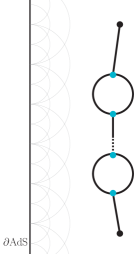
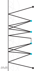
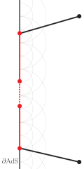
Figure 3: Left: A bulk line dressed by bubble self-energy diagrams. Center: Rewriting using the conformal spectral (i.e. split) representation. Right: Structure after integrating intermediate bulk points. Each solid red line represents a conformal bubble integral.

One Bubble Insertion

In this subsection, we work out the details of the $G^{(1)}$ term of the Born series $G=\sum^{\infty}_{n=0}G^{(n)}$ which is the term with one insertion, see Eq. (13). Computation of higher terms is similar, and the full series will be summed in next subsection.

The $G^{(1)}$ term of the series reads

$$G^{(1)}\,(z,z^{\prime}) =G^{(0)}*i\Pi*G^{(0)}\,(z,z^{\prime})$$ (54)

$$=\int_{-i\infty}^{i\infty}d\alpha\int_{-i\infty}^{i\infty}d\alpha^{\prime}\,\left(\frac{i}{k}\right)^{2}P(\alpha,\bar{\alpha})P(\alpha^{\prime},\bar{\alpha})\,\,\Omega^{(0)}_{\alpha}*i\Pi*\Omega^{(0)}_{\alpha^{\prime}}\,(z,z^{\prime})$$

with the measures

$$P(\alpha,\bar{\alpha})=\frac{1}{\alpha^{2}-\bar{\alpha}^{2}}\,,\quad P(\alpha^{\prime},\bar{\alpha})=\frac{1}{\alpha^{\prime 2}-\bar{\alpha}^{2}}\,.$$ (55)

We single out the convolution appearing in Eq. (54),

$$\Omega^{(0)}_{\alpha}*i\Pi*\Omega^{(0)}_{\alpha^{\prime}}(z,z^{\prime})=\int du\int dv\,\,\Omega^{(0)}_{\alpha}(z,u)\,i\Pi(u,v)\,\Omega^{(0)}_{\alpha^{\prime}}(v,z^{\prime})$$ (56)

and introduce the conformal spectral representation for the bubble and the external legs. We write all spectral functions in terms of the boundary-to-bulk propagators as shown in Eq. (247), giving

$$\int du\int dv\,\,\Omega_{\alpha}^{(0)}(z,u)\,i\Pi(u,v)\,\Omega_{\alpha^{\prime}}^{(0)}(v,z^{\prime})$$ (57)

$$=\left(\frac{1}{4\pi}\right)^{4}\left(\frac{\lambda}{k}\right)^{2}\int\frac{du}{(ku)^{d+1}}\int\frac{dv}{(kv)^{d+1}}\,\int_{-i\infty}^{i\infty}d\alpha_{1}\int_{-i\infty}^{i\infty}d\alpha_{2}\,P(\alpha_{1},\bar{\alpha}_{1})P(\alpha_{2},\bar{\alpha}_{2})\,\times$$

$$\int\frac{d^{d}q}{(2\pi)^{d}}{\cal K}^{+}_{\alpha}(p;z){\cal K}^{-}_{\alpha}(p;u){\cal K}^{+}_{\alpha_{1}}(q+p;u){\cal K}^{-}_{\alpha_{1}}(q+p;v){\cal K}^{+}_{\alpha_{2}}(q;v){\cal K}^{-}_{\alpha_{2}}(q;u){\cal K}^{+}_{\alpha^{\prime}}(p;v){\cal K}^{-}_{\alpha^{\prime}}(p;z^{\prime}).$$

The diagram involves products of boundary-to-bulk propagators—it corresponds to Fig. 3 (center) with a single bubble.

In $G^{(1)}$ there are two triple-K integrals, one corresponding to each vertex. Using results from App. C.5, we have

$$\int\frac{du}{(ku)^{d+1}}{\cal K}^{-}_{\alpha}(p;u){\cal K}^{+}_{\alpha_{1}}(q+p;u){\cal K}^{-}_{\alpha_{2}}(q;u)=c_{\alpha,-\alpha_{1},\alpha_{2}}k^{d/2-1}\llangle\tilde{{\cal O}}(p){\cal O}_{1}(-p-q)\tilde{\cal O}_{2}(q)\rrangle$$ (58)

$$\int\frac{dv}{(kv)^{d+1}}{\cal K}^{+}_{\alpha^{\prime}}(p;v){\cal K}^{-}_{\alpha_{1}}(q+p;v){\cal K}^{+}_{\alpha_{2}}(q;v)=c_{-\alpha^{\prime},\alpha_{1},-\alpha_{2}}k^{d/2-1}\llangle{{\cal O}}(-p)\tilde{\cal O}_{1}(p+q){\cal O}_{2}(-q)\rrangle\,\,.$$ (59)

We see that a CFT bubble integral arises in the last line of Eq. (57) when performing the intermediate bulk point integrations. This is shown in Fig. 3 (right). The evaluation of the CFT bubble in momentum space is given in Eq. (243). Both terms of the right-hand side of Eq. (243) give identical contribution by shadow symmetry ($\alpha\leftrightarrow-\alpha$).

Putting the pieces together, we have

$$\Omega^{(0)}_{\alpha}*i\Pi*\Omega^{(0)}_{\alpha^{\prime}}(z,z^{\prime})=2\delta(\alpha-\alpha^{\prime})\frac{\lambda^{2}k^{d-4}}{(4\pi)^{4}}\,2\pi{\cal B}_{\cal O}\,{\cal K}^{+}_{\alpha}(pz){\cal K}^{-}_{\alpha^{\prime}}(pz)$$ (60)

$$\quad\quad\quad\times\int d\alpha_{1}d\alpha_{2}P(\alpha_{1},\bar{\alpha}_{1})P(\alpha_{2},\bar{\alpha}_{2})c_{\alpha,-\alpha_{1},\alpha_{2}}c_{-\alpha^{\prime},\alpha_{1},-\alpha_{2}},$$

where ${\cal B}_{\cal O}$ is given in Eq. (242). In Eq. (60) we are left with two boundary-to-bulk propagators associated with the two endpoints of $G^{(1)}$. Since $\alpha=\alpha^{\prime}$ from the Dirac delta, these two boundary-to-bulk propagators can be combined into a spectral function using Eq. (247). We thus obtain

$$\Omega^{(0)}_{\alpha}*i\Pi*\Omega^{(0)}_{\alpha^{\prime}}(z,z^{\prime}) =\delta(\alpha-\alpha^{\prime})\lambda^{2}k^{d-4}\,\frac{1}{4\pi}{\cal K}^{+}_{\alpha}(pz){\cal K}^{-}_{\alpha^{\prime}}(pz)\,{\cal B}(\alpha)$$ (61)

$$=\delta(\alpha-\alpha^{\prime})\lambda^{2}k^{d-4}\,i{\cal B}(\alpha)\,\Omega^{(0)}_{\alpha}(z,z^{\prime}),$$

where we introduced the dimensionless bubble function

$${\cal B}(\alpha)=-2\frac{1}{(4\pi)^{3}}\,2\pi{\cal B}_{\cal O}\times\int d\alpha_{1}d\alpha_{2}\,P(\alpha_{1},\bar{\alpha}_{1})P(\alpha_{2},\bar{\alpha}_{2})\,c_{\alpha,-\alpha_{1},\alpha_{2}}c_{-\alpha,\alpha_{1},-\alpha_{2}}$$ (62)

$$=-\frac{1}{2^{5}\pi^{4+d/2}}\frac{1}{\Gamma(d/2)\Gamma(d/2-\alpha)\Gamma(d/2+\alpha)}\int d\alpha_{1}d\alpha_{2}\frac{\alpha_{1}\alpha_{2}\sin(\pi\alpha_{1})\sin(\pi\alpha_{2})}{(\alpha^{2}_{1}-\bar{\alpha}^{2}_{1})(\alpha^{2}_{2}-\bar{\alpha}^{2}_{2})}$$

$$\times\Gamma\left({\Smaller11\frac{\alpha+\alpha_{1}+\alpha_{2}+d/2}{2}}\right)\Gamma\left({\Smaller11\frac{\alpha-\alpha_{1}+\alpha_{2}+d/2}{2}}\right)\Gamma\left({\Smaller11\frac{\alpha+\alpha_{1}-\alpha_{2}+d/2}{2}}\right)\Gamma\left({\Smaller11\frac{-\alpha+\alpha_{1}+\alpha_{2}+d/2}{2}}\right)$$

$$\times\Gamma\left({\Smaller11\frac{-\alpha-\alpha_{1}-\alpha_{2}+d/2}{2}}\right)\Gamma\left({\Smaller11\frac{-\alpha+\alpha_{1}-\alpha_{2}+d/2}{2}}\right)\Gamma\left({\Smaller11\frac{-\alpha-\alpha_{1}+\alpha_{2}+d/2}{2}}\right)\Gamma\left({\Smaller11\frac{\alpha-\alpha_{1}-\alpha_{2}+d/2}{2}}\right)$$

This bubble function is proportional to the one obtained in Giombi:2017hpr . An additional cross-check is obtained further below.

In Eq. (61) we have reduced the convolutions in $G^{(1)}$ into a nontrivial algebraic factor. We complete the evaluation by putting Eq. (61) back into Eq. (54), which gives

$$G^{(1)}\,(z,z^{\prime})=G^{(0)}*i\Pi*G^{(0)}\,(z,z^{\prime})$$ (63)

$$=\int_{-i\infty}^{i\infty}d\alpha\int_{-i\infty}^{i\infty}d\alpha^{\prime}\,\left(\frac{i}{k}\right)^{2}P(\alpha,\bar{\alpha})P(\alpha^{\prime},\bar{\alpha})\,\,\delta(\alpha-\alpha^{\prime})\lambda^{2}k^{d-4}i{\cal B}(\alpha)\Omega^{(0)}_{\alpha}\,(z,z^{\prime})$$

$$=\frac{i}{k}\int_{-i\infty}^{i\infty}d\alpha\,P^{2}(\alpha,\bar{\alpha})\,\left[-\hat{\lambda}^{2}{\cal B}(\alpha)\right]\Omega^{(0)}_{\alpha}\,(z,z^{\prime}).$$

The Spectral Born Series

The above steps can be reproduced for an arbitrary number of bubble insertions. One finds the $n$-bubble contribution to be

$$G^{(n)}\,(z,z^{\prime})=\frac{i}{k}\int_{-i\infty}^{i\infty}d\alpha\,P(\alpha,\bar{\alpha})\,\left[-\hat{\lambda}^{2}P(\alpha,\bar{\alpha}){\cal B}(\alpha)\right]^{n}\Omega^{(0)}_{\alpha}\,(z,z^{\prime}).$$ (64)

We see that a geometric series appears and hence the full Born sum can be performed. This is because spectral transforms turn convolutions into products, as discussed in Carmi:2018qzm . Here we have recovered this feature via direct calculation. There is no analog to this property in the momentum spectral representation, because unlike in the conformal representation the bubble integral does not conserve the spectral variable $\hat{p}$.

Summing the Born series, we find that the complete dressed propagator in the conformal spectral representation is

$$\sum_{n=0}^{\infty}G^{(n)}\,(z,z^{\prime})=G\,(z,z^{\prime})=\left(\frac{i}{k}\right)\int_{-i\infty}^{i\infty}d\alpha\,\frac{1}{P(\alpha,\bar{\alpha})^{-1}+\hat{\lambda}^{2}{\cal B}(\alpha)}\Omega^{(0)}_{\alpha}\,(z,z^{\prime})\,.$$ (65)

Thus it turns out that in the conformal spectral representation the dressing amounts to a deformation of the $P(\alpha,\bar{\alpha})$ measure and $\hat{\lambda}^{2}{\cal B}(\alpha)$ effectively has the role of a “spectral self-energy”. In particular we can see that the $\alpha=\pm\bar{\alpha}$ poles of the free spectral function $P(\alpha,\bar{\alpha})$ get shifted by the $\hat{\lambda}^{2}{\cal B}(\alpha)$ term.

Aside: Anomalous Dimension from the Dressed Propagator

For sufficiently small coupling $\hat{\lambda}\ll 1$ we can approximate ${\cal B}(\alpha)\approx{\cal B}(\bar{\alpha})$ near the $\alpha=\pm\bar{\alpha}$ poles. Other poles exist whenever $\hat{\lambda}\neq 0$, but the corresponding residues are expected to be small for $\hat{\lambda}\ll 1$ and are not our focus.  The ${\cal B}(\bar{\alpha})$ constant can be seen as a correction to the bulk mass,

$$m^{2}_{\Phi}|_{\rm dressed}=\left(\bar{\alpha}^{2}-\frac{d^{2}}{4}-{\cal B}(\bar{\alpha})\right)k^{2}\,.$$ (66)

In the dual CFT, the correction amounts to an anomalous dimension $\gamma$ shifting the conformal dimensions $\Delta_{\pm}$. We define $\gamma$ such that

$$\Delta_{\pm}|_{\rm dressed}=\Delta_{\pm}\pm\gamma=\frac{d}{2}\pm\bar{\alpha}\pm\gamma\,,$$ (67)

with

$$\gamma=-\frac{{\cal B}(\bar{\alpha})}{2\bar{\alpha}}\,.$$ (68)

The fact that the sign of the correction flips between $\Delta_{+}$ and $\Delta_{-}$ is enforced from the AdS side since it is a correction on $\bar{\alpha}$ and since $\Delta_{\pm}=\frac{d}{2}\pm\bar{\alpha}$. The sign flip is also clear from the CFT side in order for shadow symmetry to be respected.

We find that the imaginary part of ${\cal B}(\bar{\alpha})$ vanishes. To note this, close the contours in Eq. (62) and use the residue theorem. The residues are real and hence by counting factors of $i$, we determine that ${\cal B}(\bar{\alpha})$ is purely real. This is consistent with the conclusions in Giombi:2017hpr . Thus the leading correction to $\bar{\alpha}$ is purely real.

We find that our result Eq. (68) precisely matches the anomalous dimension found in Giombi:2017hpr (Eq. (2.37) in that reference). In that reference the anomalous dimension was evaluated by looking at the $\log(\Delta X)$ term in a on-shell bubble amplitude in position space. Here we have confirmed their result with a different approach. From Eq. (65) other higher order effects such as wave-function renormalization could be studied.

The Self-Energy as a Spectral Transform

To obtain a useful form of $\Pi$ in the conformal spectral representation, we apply the EOM operator $\cal D$ on both sides of $G^{(1)}(z,z^{\prime})=G^{(0)}*i\Pi*G^{(0)}(z,z^{\prime})$. Using the free EOM Eq. (17), we obtain

$${\cal D}_{z}{\cal D}_{z^{\prime}}G^{(1)}(z,z^{\prime})=-i\frac{1}{\sqrt{|\gamma|}_{z}\sqrt{|\gamma|}_{z^{\prime}}}\Pi(z,z^{\prime})=-i(kz)^{d+1}(kz^{\prime})^{d+1}\Pi(z,z^{\prime}).$$ (69)

$G^{(1)}$ in the conformal spectral representation has been computed in Eq. (63). Using it in Eq. (69) gives

$${\cal D}_{z}{\cal D}_{z^{\prime}}G^{(1)}(z,z^{\prime}) =\frac{i}{k}\int_{-i\infty}^{i\infty}d\alpha\,P^{2}(\alpha,\bar{\alpha})\,\left[-\hat{\lambda}^{2}{\cal B}(\alpha)\right]{\cal D}_{z}{\cal D}_{z^{\prime}}\Omega^{(0)}_{\alpha}\,(z,z^{\prime})$$ (70)

$$=-ik^{3}\int_{-i\infty}^{i\infty}d\alpha\,\,\hat{\lambda}^{2}{\cal B}(\alpha)\Omega^{(0)}_{\alpha}\,(z,z^{\prime})\,.$$

In doing so we have thus obtained

$$i(kz)^{d+1}(kz^{\prime})^{d+1}\Pi(z,z^{\prime})=i\hat{\lambda}^{2}k^{3}\int_{-i\infty}^{i\infty}d\alpha\,{\cal B}(\alpha)\Omega^{(0)}_{\alpha}\,(z,z^{\prime})\,.$$ (71)

This establishes that $\hat{\lambda}^{2}k^{3}{\cal B}(\alpha)$ is the spectral transform of $(k^{2}zz^{\prime})^{d+1}\Pi$. This is the form of the self-energy that we will use in the conformal spectral calculation of Sec. 4.2.

Representations and Properties of ${\rm Im}\Pi$

In this section we evaluate a self-energy bubble diagram $i\Pi$ in the three different representation shown in Sec. 2. Our focus is on the imaginary part ${\rm Im}\Pi$. The equivalence of the expressions in various representations is nontrivial, hence we demonstrate it explicitly in Sec. 4.4. The various representations render manifest different properties of the self-energy. These properties are discussed in Sec. 4.5.

Throughout this section the interaction considered is a cubic coupling between three inequivalent real scalar fields

$$S\supset\int dX^{M}\sqrt{|\gamma|}\lambda\Phi\Phi_{1}\Phi_{2}\,.$$ (72)

We introduce $\alpha_{1,2}$ to parameterize the bulk masses of the $\Phi_{1,2}$ fields. When working in the conformal spectral representation, we change our convention $\alpha_{1,2}\rightarrow\bar{\alpha}_{1,2}$ as done in Sec. 3. Our results are trivially extended to a cubic self-interaction via the operator $\frac{\lambda}{3!}\Phi^{3}$ and taking into account a $\frac{1}{2}$ symmetry factor in the loop.

In our calculations, we focus on $p^{2}$ close to the real line. For $p^{2}\in\mathbb{R_{-}}$, we are permitted to stay exactly on the real line. The propagator has a branch cut for timelike momentum however, so taking $p^{2}\in\mathbb{R_{+}}$ is not well defined (see Sec. 2.2). Instead, one must give $p^{2}$ a small imaginary part $p^{2}\rightarrow p^{2}+i\epsilon$ to resolve the branch ambiguity. We allow for either $\epsilon>0$ or $\epsilon<0$ in our calculations. We show in Sec. 4.5 that the sign of $\epsilon$ controls the sign of ${\rm Im}\Pi$.

The self-energy of $\Phi$ is given by

$$\Pi_{p}(z,z^{\prime})=\frac{i\lambda^{2}}{\left(k^{2}zz^{\prime}\right)^{d+1}}\int\frac{d^{d}q}{(2\pi)^{d}}G^{(0)}_{1}(p+q,z,z^{\prime})G^{(0)}_{2}(q,z^{\prime},z).$$ (73)

Eq. (73) serves as the starting point for the following calculations.

${\rm Im}\Pi$ in the Canonical Representation

We substitute the canonical propagator Eq. (23) into Eq. (73) and use the infinite series-representations of the Bessel functions,

$$I_{\alpha}(\sqrt{-p^{2}}z)= \sum_{m=0}^{\infty}\frac{1}{m!\Gamma(m+\alpha+1)}\left(\frac{\sqrt{-p^{2}}z}{2}\right)^{2m+\alpha}$$ (74)

$$K_{\alpha}(\sqrt{-p^{2}}z)= \frac{\pi}{2\sin(\pi\alpha)}\sum_{m=0}\frac{1}{m!}\left(\frac{\sqrt{-p^{2}}z}{2}\right)^{2m}\times$$ (75)

$$\left[\frac{1}{\Gamma(m-\alpha+1)}\left(\frac{\sqrt{-p^{2}}z}{2}\right)^{-\alpha}-\frac{1}{\Gamma(m+\alpha+1)}\left(\frac{\sqrt{-p^{2}}z}{2}\right)^{\alpha}\right].$$

In this representation, the self-energy is

$$\Pi_{p}(z,z^{\prime})=\frac{-i\pi^{2}\lambda^{2}}{4k^{4}zz^{\prime}\sin(\pi\alpha_{1})\sin(\pi\alpha_{2})}\int\frac{d^{d}q}{(2\pi)^{d}}\sum_{s,t=0}^{\infty}\sum_{n,m=0}^{\infty}\frac{(-1)^{n+m+s+t}}{n!m!s!t!}\,\times$$ (76)

$$\frac{1}{\Gamma(n+\alpha_{2}+1)}\frac{1}{\Gamma(s+\alpha_{1}+1)}\left(\frac{qz_{<}}{2}\right)^{2s+\alpha_{1}}\left(\frac{(p+q)z_{<}}{2}\right)^{2n+\alpha_{2}}\left(\frac{qz_{>}}{2}\right)^{2t}\left(\frac{(p+q)z_{>}}{2}\right)^{2m}~{}\times$$

$$\left[\frac{\left(\frac{\vphantom{(}qz_{>}}{2}\right)^{-\alpha_{1}}}{\Gamma(t-\alpha_{1}+1)}-\frac{\left(\frac{\vphantom{(}qz_{>}}{2}\right)^{\alpha_{1}}e^{-i\alpha_{1}\pi\text{Sign}(\epsilon)}}{\Gamma(t+\alpha_{1}+1)}\right]\left[\frac{\left(\frac{(p+q)z_{>}}{2}\right)^{-\alpha_{2}}}{\Gamma(m-\alpha_{2}+1)}-\frac{\left(\frac{(p+q)z_{>}}{2}\right)^{\alpha_{2}}e^{-i\alpha_{2}\pi\text{Sign}(\epsilon)}}{\Gamma(m+\alpha_{2}+1)}\right].$$

$\Pi_{p}(z,z^{\prime})$ contains many terms, each of which go like

$$\Pi_{p}(z,z^{\prime})\sim\int\frac{d^{d}q}{(2\pi)^{d}}\left(\left(p+q\right)^{2}\right)^{a}\left(q^{2}\right)^{b}$$ (77)

for some $a,b$. To each term, we apply the identity

$$\left(\left(p+q\right)^{2}\right)^{a}\left(q^{2}\right)^{b}=\int_{0}^{1}dx\frac{(x\left(p+q\right)^{2}+(1-x)q^{2})^{a+b}}{x^{a+1}(1-x)^{b+1}}\frac{\Gamma(-a-b)}{\Gamma(-a)\Gamma(-b)}\,.$$ (78)

The integral on the right-hand side converges for ${\rm Re}(a),{\rm Re}(b)<0$. However, provided the final result of the calculation is analytic in $a,b$, the result can be extended by analytical continuation such that restrictions on $a,b$ are ultimately lifted. 

Shifting the loop momentum $l\equiv q+px$, we obtain

$$\Pi_{p}(z,z^{\prime})\sim\int_{0}^{1}dx\int\frac{d^{d}l}{(2\pi)^{d}}\frac{(l^{2}+x(1-x)p^{2})^{a+b}}{x^{a+1}(1-x)^{b+1}}\frac{\Gamma(-a-b)}{\Gamma(-a)\Gamma(-b)}.$$ (79)

We evaluate the loop integral with

$$\int\frac{d^{d}l}{(2\pi)^{d}}\left(l^{2}+\Delta\right)^{c}=\frac{i(-i\text{Sign}(\epsilon))^{d}}{(4\pi)^{\frac{d}{2}}}\frac{\Gamma\left(-c-\frac{d}{2}\right)}{\Gamma(-c)}\Delta^{c+\frac{d}{2}}\,.$$ (80)

Again, the loop integrals are performed in the domain of $(c,d)$ where the integral on the left-hand-side converges. The functions on the right-hand-side are analytic in $c$ anywhere away from $c$ integer, hence the final result will be ultimately analytically continued in $c$. The particular points where a divergence appear require renormalization. However such divergences are in the real part of $\Pi$ and are irrelevant for the study of ${\rm Im}\Pi$.

Putting Eqs. (78) and (80) together yields

$$\Pi_{p}(z,z^{\prime})\sim\frac{i(-i\text{Sign}(\epsilon))^{d}}{(4\pi)^{\frac{d}{2}}}\left(p^{2}\right)^{a+b+\frac{d}{2}}\frac{\Gamma\left(-a-b-\frac{d}{2}\right)}{\Gamma(-a)\Gamma(-b)}\int_{0}^{1}dxx^{b+\frac{d}{2}-1}(1-x)^{a+\frac{d}{2}-1}.$$ (81)

We identify the remaining integral as being the integral representation of the Beta function. Evaluating the integral, we obtain 

$$\Pi_{p}(z,z^{\prime})\sim\frac{i(-i\text{Sign}(\epsilon))^{d}}{(4\pi)^{d/2}}\left(p^{2}\right)^{a+b+d/2}\frac{\Gamma(-a-b-d/2)}{\Gamma(-a)\Gamma(-b)}\frac{\Gamma(a+d/2)\Gamma(b+d/2)}{\Gamma(a+b+d)}.$$ (82)

There are four terms in Eq. (76) corresponding to the four sign pairings of $\alpha_{1},\alpha_{2}$ in the exponents. All but the $z_{>}^{\alpha_{1}+\alpha_{2}}$ term have either $a\in\mathbb{N}$ or $b\in\mathbb{N}$ or both. These terms vanish trivially on account of the $\Gamma(-a)\Gamma(-b)$ function in the denominator of Eq. (82). The disappearance of the $z_{>}^{-\alpha_{1}-\alpha_{2}}$ term can also be shown by taking the imaginary part of $\Pi$. In particular for even $d$ when $\Gamma(-a-b-d/2)$ diverges, we find that the $z_{>}^{-\alpha_{1}-\alpha_{2}}$ term is purely real.

Making everything explicit again and taking the imaginary part, we have

$$\text{Im}\Pi_{p}(z,z^{\prime})=$$ (83)

$$\text{Im}\Bigg{[}\frac{\pi^{2}\lambda^{2}p^{d}e^{-i\pi\left(\alpha_{1}+\alpha_{2}+d/2\right)\text{Sign}(\epsilon)}}{4k^{4}zz^{\prime}\sin(\pi\alpha_{1})\sin(\pi\alpha_{2})(4\pi)^{d/2}}\sum_{s,t=0}^{\infty}\sum_{n,m=0}^{\infty}\left(\frac{pz}{2}\right)^{2n+2s+\alpha_{1}+\alpha_{2}}\left(\frac{pz^{\prime}}{2}\right)^{2m+2t+\alpha_{1}+\alpha_{2}}\times$$

$$\quad\quad\frac{(-1)^{s}}{s!\Gamma(s+\alpha_{1}+1)}\frac{(-1)^{t}}{t!\Gamma(t+\alpha_{1}+1)}\frac{(-1)^{n}}{n!\Gamma(n+\alpha_{2}+1)}\frac{(-1)^{m}}{m!\Gamma(m+\alpha_{2}+1)}\,\times$$

$$\quad\quad\frac{\Gamma(-n-m-s-t-\alpha_{1}-\alpha_{2}-d/2)}{\Gamma(-n-m-\alpha_{2})\Gamma(-s-t-\alpha_{1})}\frac{\Gamma(s+t+\alpha_{1}+d/2)\Gamma(n+m+\alpha_{2}+d/2)}{\Gamma(s+t+n+m+d+\alpha_{1}+\alpha_{2})}\Bigg{]}\,,$$

where we removed the $<,>$ subscripts because the expression is symmetric upon relabeling. We regroup the complex exponential with the factors of $p$ in Eq. (83) to make the $\sqrt{-p^{2}}$ factor appear explicitly. This involves reabsorbing the $i\epsilon$ into $p^{2}$, where it remains implicitly, yielding

$$\text{Im}\Pi_{p} (z,z^{\prime})=\sum_{n,m,s,t=0}^{\infty}\frac{\lambda^{2}\pi^{2}}{4\pi^{d/2}k^{4}\left(zz^{\prime}\right)^{1+d/2}\sin(\pi\alpha_{1})\sin(\pi\alpha_{2})}\times$$ (84)

$$\frac{(-1)^{s}}{s!\Gamma(s+\alpha_{1}+1)}\frac{(-1)^{t}}{t!\Gamma(t+\alpha_{1}+1)}\frac{(-1)^{n}}{n!\Gamma(n+\alpha_{2}+1)}\frac{(-1)^{m}}{m!\Gamma(m+\alpha_{2}+1)}\times$$

$$\frac{\Gamma(-n-m-s-t-\alpha_{1}-\alpha_{2}-d/2)}{\Gamma(-n-m-\alpha_{2})\Gamma(-s-t-\alpha_{1})}\frac{\Gamma(s+t+\alpha_{1}+d/2)\Gamma(n+m+\alpha_{2}+d/2)}{\Gamma(s+t+n+m+d+\alpha_{1}+\alpha_{2})}~{}\times$$

$$\text{Im}\Bigg{[}\left(\Smaller11\frac{\sqrt{-p^{2}}z}{2}\right)^{2n+2s+\alpha_{1}+\alpha_{2}+d/2}\left(\Smaller11\frac{\sqrt{-p^{2}}z^{\prime}}{2}\right)^{2m+2t+\alpha_{1}+\alpha_{2}+d/2}\Bigg{]}.$$

In this form, $\text{Im}\Pi_{p}(z,z^{\prime})$ explicitly vanishes for spacelike momentum. Using Euler’s reflection formula

$$\Gamma(x)\Gamma(1-x)=\frac{\pi}{\sin(\pi x)}\quad\text{for}\quad x\not\in\mathbb{Z},$$ (85)

and taking the imaginary part, Eq. (84) can be written as

$$\text{Im}\Pi_{p} (z,z^{\prime})=$$ (86)

$$\frac{\text{Sign}(\epsilon)\pi\lambda^{2}p^{d}}{4k^{4}zz^{\prime}(4\pi)^{d/2}}\sum_{n,m,s,t=0}^{\infty}\left(\frac{pz}{2}\right)^{2n+2s+\alpha_{1}+\alpha_{2}}\left(\frac{pz^{\prime}}{2}\right)^{2m+2t+\alpha_{1}+\alpha_{2}}\times$$

$$\frac{(-1)^{s}}{s!\Gamma(s+\alpha_{1}+1)}\frac{(-1)^{t}}{t!\Gamma(t+\alpha_{1}+1)}\frac{(-1)^{n}}{n!\Gamma(n+\alpha_{2}+1)}\frac{(-1)^{m}}{m!\Gamma(m+\alpha_{2}+1)}~{}\times$$

$$\frac{\Gamma(n+m+\alpha_{2}+1)\Gamma(s+t+\alpha_{1}+1)}{\Gamma(n+m+s+t+\alpha_{1}+\alpha_{2}+d/2+1)}\frac{\Gamma(s+t+\alpha_{1}+d/2)\Gamma(n+m+\alpha_{2}+d/2)}{\Gamma(s+t+n+m+d+\alpha_{1}+\alpha_{2})}.$$

Eq. (86) represents our final result for $\text{Im}\Pi_{p}(z,z^{\prime})$ in the canonical representation.

${\rm Im}\Pi$ in the Conformal Spectral Representation

Some preliminary work was done in Sec. 3 to calculate ${\rm Im}\Pi$ in the conformal spectral representation. Here we start from the identity Eq. (71), repeated here:

$${\rm Im}(k^{2}zz^{\prime})^{d+1}\Pi(z,z^{\prime})={\rm Im}\left[\hat{\lambda}^{2}k^{3}\int_{-i\infty}^{i\infty}d\alpha\,{\cal B}(\alpha)\Omega^{(0)}_{\alpha}\,(z,z^{\prime})\right].$$ (87)

In this subsection only, we follow the convention of Sec. 3 and use $\alpha,\alpha_{1},\alpha_{2}$ to denote integration variables. We use $\bar{\alpha}_{1},\bar{\alpha}_{2}$ for the bulk mass parameters, Eq. (8). We expand the Bessel functions in a series using Eq. (75) and use the $\alpha\leftrightarrow-\alpha$ shadow symmetry of the integrand to write the four terms in $\Omega^{(0)}_{\alpha}\,(z,z^{\prime})$ as two. We have

$${\rm Im}\Pi(z,z^{\prime})=$$ (88)

$${\rm Im}\Bigg{[}\frac{i\hat{\lambda}^{2}k^{3}}{\left(k^{2}zz^{\prime}\right)^{d/2+1}}\int_{-i\infty}^{i\infty}d\alpha\,{\cal B}(\alpha)\frac{\alpha}{2\sin(\pi\alpha)}\sum_{m,n=0}^{\infty}\frac{1}{m!n!}\left(\Smaller11\frac{\sqrt{-p^{2}}z^{\prime}}{2}\right)^{2n}\left(\Smaller11\frac{\sqrt{-p^{2}}z}{2}\right)^{2m}\times$$

$$\frac{1}{\Gamma(n-\alpha+1)}\left(\Smaller11\frac{\sqrt{-p^{2}}z^{\prime}}{2}\right)^{-\alpha}\left(\frac{1}{\Gamma(m-\alpha+1)}\left(\Smaller11\frac{\sqrt{-p^{2}}z}{2}\right)^{-\alpha}-\frac{1}{\Gamma(m+\alpha+1)}\left(\Smaller11\frac{\sqrt{-p^{2}}z}{2}\right)^{\alpha}\right)\Bigg{]}.$$

The imaginary part of the above expression will ultimately come from $\text{Im}\left(-p^{2}\right)^{a}$ for some $a$. That is, all other factors of $i$ from applications of the residue theorem conspire to produce a real prefactor. In the second term of Eq. (88) above, the two powers of $\alpha$ cancel, and hence $a$ is necessarily an integer. Thus we find that this second term vanishes upon taking the imaginary part, as it is purely real. The poles from the $1/\sin(\pi\alpha)$ factor sit at integer $\alpha$, which again yields integer $a$ upon applying the residue theorem. Hence these residues do not contribute to ${\rm Im}\Pi(z,z^{\prime})$.

Following this preliminary result, only the first term in the bracket in Eq. (88) contributes to the imaginary part, and only the poles within the bubble function ${\cal B}(\alpha)$ are relevant. We close the $\alpha$-contour towards the negative reals, where the integrand vanishes exponentially on account of the Gamma functions. This selects an infinite number of residues from the four relevant Gamma functions within the bubble function, Eq. (62). The sets of poles that we enclose are located at

$$\alpha=\pm\alpha_{1}\pm\alpha_{2}-\frac{d}{2}-2l\quad\quad\quad\text{for}\quad\quad\quad l\in\mathbb{N}\,.$$ (89)

The corresponding four sets of residues all take the same form, but with relative sign flips ($\alpha_{1}\leftrightarrow-\alpha_{1}$ and/or $\alpha_{2}\leftrightarrow-\alpha_{2}$). We have

$${\rm Im}\Pi(z,z^{\prime})={\rm Im}\sum_{m,n,l=0}^{\infty}\int d\alpha_{1}d\alpha_{2}\left(\mathcal{I}_{\alpha_{1},\alpha_{2}}+\mathcal{I}_{-\alpha_{1},\alpha_{2}}+\mathcal{I}_{\alpha_{1},-\alpha_{2}}+\mathcal{I}_{-\alpha_{1},-\alpha_{2}}\right)$$ (90)

for

$$\mathcal{I}_{\alpha_{1},\alpha_{2}}\equiv$$ (91)

$$\frac{\hat{\lambda}^{2}k^{3}}{\left(k^{2}zz^{\prime}\right)^{d/2+1}}\left(\frac{\sqrt{-p^{2}}z}{2}\right)^{2m+2l+\alpha_{1}+\alpha_{2}+d/2}\left(\frac{\sqrt{-p^{2}}z^{\prime}}{2}\right)^{2n+2l+\alpha_{1}+\alpha_{2}+d/2}\times$$

$$\frac{1}{2^{4}\pi^{1+d/2}}\frac{1}{l!m!n!}\frac{(2l+\alpha_{1}+\alpha_{2}+d/2)\csc(\pi(\alpha_{1}+\alpha_{2}+d/2))}{\Gamma(d/2)\Gamma(2l+\alpha_{1}+\alpha_{2}+d)\Gamma(l+\alpha_{1}+\alpha_{2}+1)}\frac{\alpha_{1}\alpha_{2}}{(\alpha^{2}_{1}-\bar{\alpha}^{2}_{1})(\alpha^{2}_{2}-\bar{\alpha}^{2}_{2})}\times$$

$$\frac{\Gamma\left(l+d/2\right)\Gamma\left(l+\alpha_{1}+d/2\right)\Gamma\left(l+\alpha_{2}+d/2\right)\Gamma\left(2l+\alpha_{1}+\alpha_{2}+1\right)\Gamma\left(l+\alpha_{1}+\alpha_{2}+d/2\right)}{\Gamma(n+2l+\alpha_{1}+\alpha_{2}+d/2+1)\Gamma(m+2l+\alpha_{1}+\alpha_{2}+d/2+1)\Gamma\left(l+\alpha_{1}+1\right)\Gamma\left(l+\alpha_{2}+1\right)},$$

where we have simplified the expression by using the reflection formula Eq. (85). All four terms are equivalent—as can be seen by $\alpha_{j}\rightarrow-\alpha_{j}$ relabelings—and hence the integrand amounts to $4\mathcal{I}_{\alpha_{1},\alpha_{2}}$.

We then perform the $\alpha_{1}$ and $\alpha_{2}$ integrals. We close the integrals towards the positive reals, where the integrand vanishes exponentially on account of the Gamma functions. Within the contour, there are poles at $\alpha_{i}=\bar{\alpha}_{i}$ from the $P\left(\bar{\alpha}_{i},\alpha_{i}\right)$ measures (see Eq. (55)) and poles at $\alpha_{1}+\alpha_{2}+d/2\in\mathbb{Z}_{+}$ from $\csc(\pi(\alpha_{1}+\alpha_{2}+d/2))$. The residues from the cosecant only give a contribution to ${\rm Re}\Pi(z,z^{\prime})$ because they give rise to even powers of $\sqrt{-p^{2}}$. The residues from the $P\left(\bar{\alpha}_{i},\alpha_{i}\right)$ measures yield a contribution to ${\rm Im}\Pi(z,z^{\prime})$.

We obtain

$${\rm Im}\Pi(z,z^{\prime}) =-\sum_{m,n,l=0}^{\infty}\frac{\hat{\lambda}^{2}k^{3}}{\left(k^{2}zz^{\prime}\right)^{d/2+1}}\frac{1}{2^{2}\pi^{d/2-1}}\frac{1}{l!m!n!}\times$$ (92)

$$\frac{\Gamma\left(l+\bar{\alpha}_{1}+\bar{\alpha}_{2}+d/2\right)(2l+\bar{\alpha}_{1}+\bar{\alpha}_{2}+d/2)\csc(\pi(\bar{\alpha}_{1}+\bar{\alpha}_{2}+d/2))}{\Gamma(d/2)\Gamma(n+2l+\bar{\alpha}_{1}+\alpha_{2,0}+d/2+1)\Gamma(m+2l+\bar{\alpha}_{1}+\bar{\alpha}_{2}+d/2+1)}\times$$

$$\frac{\Gamma\left(l+d/2\right)\Gamma\left(l+\bar{\alpha}_{1}+d/2\right)\Gamma\left(l+\bar{\alpha}_{2}+d/2\right)\Gamma\left(2l+\bar{\alpha}_{1}+\bar{\alpha}_{2}+1\right)}{\Gamma(2l+\bar{\alpha}_{1}+\bar{\alpha}_{2}+d)\Gamma(l+\bar{\alpha}_{1}+\bar{\alpha}_{2}+1)\Gamma\left(l+\bar{\alpha}_{1}+1\right)\Gamma\left(l+\bar{\alpha}_{2}+1\right)}\times$$

$${\rm Im}\left[\left(\Smaller11\frac{\sqrt{-p^{2}}z}{2}\right)^{2m+2l+\bar{\alpha}_{1}+\bar{\alpha}_{2}+d/2}\left(\Smaller11\frac{\sqrt{-p^{2}}z^{\prime}}{2}\right)^{2n+2l+\bar{\alpha}_{1}+\bar{\alpha}_{2}+d/2}\right]\,.$$

The self-energy becomes real for spacelike momenta, which is straightforward to note in this form. For timelike momenta, the imaginary part is given by

$${\rm Im}\Pi(z,z^{\prime})=$$ (93)

$$\text{Sign}\left(\epsilon\right)\sum_{m,n,l=0}^{\infty}\frac{(-1)^{n+m}}{m!n!l!}\left(\frac{pz}{2}\right)^{2m+2l+\bar{\alpha}_{1}+\bar{\alpha}_{2}+d/2}\left(\frac{pz^{\prime}}{2}\right)^{2n+2l+\bar{\alpha}_{1}+\bar{\alpha}_{2}+d/2}\times$$

$$\frac{\hat{\lambda}^{2}k^{3}}{2^{2}\pi^{d/2-1}\left(k^{2}zz^{\prime}\right)^{d/2+1}}\frac{\Gamma\left(l+d/2\right)\Gamma\left(l+\bar{\alpha}_{1}+d/2\right)\Gamma\left(l+\bar{\alpha}_{2}+d/2\right)\Gamma\left(2l+\bar{\alpha}_{1}+\bar{\alpha}_{2}+1\right)}{\Gamma(d/2)\Gamma(2l+\bar{\alpha}_{1}+\bar{\alpha}_{2}+d)\Gamma(l+\bar{\alpha}_{1}+\bar{\alpha}_{2}+1)}\times$$

$$\frac{(2l+\bar{\alpha}_{1}+\bar{\alpha}_{2}+d/2)\Gamma\left(l+\bar{\alpha}_{1}+\bar{\alpha}_{2}+d/2\right)}{\Gamma\left(l+\bar{\alpha}_{1}+1\right)\Gamma\left(l+\bar{\alpha}_{2}+1\right)\Gamma(n+2l+\bar{\alpha}_{1}+\bar{\alpha}_{2}+d/2+1)\Gamma(m+2l+\bar{\alpha}_{1}+\bar{\alpha}_{2}+d/2+1)}\,.$$

We recognize the sums over $n,m$ as the series representation of the Bessel function $J$,

$$J_{2l+\bar{\alpha}_{1}+\bar{\alpha}_{2}+d/2}\left(x\right)=\sum_{j=0}^{\infty}\frac{(-1)^{j}\left(\frac{x}{2}\right)^{2j+2l+\bar{\alpha}_{1}+\bar{\alpha}_{2}+d/2}}{j!\Gamma(j+2l+\bar{\alpha}_{1}+\bar{\alpha}_{2}+d/2+1)}.$$ (94)

This gives

$${\rm Im}\Pi(z,z^{\prime})=$$ (95)

$$\frac{\text{Sign}\left(\epsilon\right)\hat{\lambda}^{2}k^{3}}{2^{2}\pi^{d/2-1}\left(k^{2}zz^{\prime}\right)^{d/2+1}}\sum_{l=0}^{\infty}(2l+\bar{\alpha}_{1}+\bar{\alpha}_{2}+d/2)J_{2l+\bar{\alpha}_{1}+\bar{\alpha}_{2}+d/2}\left(pz\right)J_{2l+\bar{\alpha}_{1}+\bar{\alpha}_{2}+d/2}\left(pz^{\prime}\right)\times$$

$$\frac{\Gamma\left(l+d/2\right)\Gamma\left(l+\bar{\alpha}_{1}+d/2\right)\Gamma\left(l+\bar{\alpha}_{2}+d/2\right)\Gamma\left(2l+\bar{\alpha}_{1}+\bar{\alpha}_{2}+1\right)\Gamma\left(l+\bar{\alpha}_{1}+\bar{\alpha}_{2}+d/2\right)}{\Gamma(d/2)\Gamma(l+1)\Gamma(2l+\bar{\alpha}_{1}+\bar{\alpha}_{2}+d)\Gamma(l+\bar{\alpha}_{1}+\bar{\alpha}_{2}+1)\Gamma\left(l+\bar{\alpha}_{1}+1\right)\Gamma\left(l+\bar{\alpha}_{2}+1\right)}\,.$$

Eq. (95) represents our final result for $\text{Im}\Pi_{p}(z,z^{\prime})$ in the conformal spectral representation. In Sec. 4.5.3, we identify this result as being a sum over the imaginary part of propagators.

${\rm Im}\Pi$ in the Momentum Spectral Representation

We again start from Eq. (73) and express the propagator in the $p$-spectral representation, Eq. (34). We introduce a Feynman parameter and shift the loop momentum, $l\equiv q+px$. This yields

$$\Pi_{p}(z,z^{\prime})=\frac{-i\lambda^{2}}{\left(k^{2}zz^{\prime}\right)^{d+1}}\int_{0}^{1}dx\int_{0}^{\infty}dm_{1}\Omega_{m_{1}}(z,z^{\prime})\int_{0}^{\infty}dm_{2}\Omega_{m_{2}}(z,z^{\prime})\int\frac{d^{d}l}{(2\pi)^{d}}\frac{1}{\left(l^{2}-\Delta\right)^{2}}$$ (96)

for

$$\Delta\equiv xm_{2}^{2}+(1-x)m_{1}^{2}-x(1-x)p^{2}.$$ (97)

We evaluate the loop integral in arbitrary dimension with

$$\int\frac{d^{d}l}{(2\pi)^{d}}\frac{1}{(l^{2}-\Delta)^{2}} =\frac{i\Gamma\left(2-\frac{d}{2}\right)}{(4\pi)^{d/2}}\Delta^{d/2-2}\,.$$ (98)

The left-hand side integral converges for $d<4$. However it can be analytically continued in $d$. For odd $d$, we write the square root as

$$\left.\sqrt{\Delta}\right|_{\text{Re}\Delta\gg\text{Im}\Delta}\approx i\sqrt{\left|\Delta\right|}\Theta\left(-\text{Re}\Delta\right)\text{Sign}\left(\text{Im}\Delta\right)+\sqrt{\left|\Delta\right|}\Theta\left(\text{Re}\Delta\right)\,,$$ (99)

valid for $\Delta$ near the real line. For even $d$, we take $d=d_{0}\pm\varepsilon$ for $\varepsilon\ll 1$ and use the reflection formula Eq. (85). We obtain

$$\left.\int\frac{d^{d}l}{(2\pi)^{d}}\frac{1}{(l^{2}-\Delta)^{2}}\right|_{d_{0}\text{ even}} =\frac{i\pi(-1)^{d_{0}/2-1}}{(4\pi)^{d_{0}/2}\sin\left(\pm\frac{\pi\varepsilon}{2}\right)\Gamma\left(\frac{d_{0}}{2}-1\right)}\Delta^{d_{0}/2-2}\Delta^{\pm\varepsilon/2}\,.$$ (100)

We expand Eq. (100) for $\varepsilon\ll 1$ using

$$\Delta^{\pm\varepsilon/2}\approx 1+\pm\frac{\varepsilon}{2}\log\Delta\,,\quad\quad\sin\left(\pm\frac{\pi\varepsilon}{2}\right)\approx\pm\frac{\pi\varepsilon}{2}.$$ (101)

We note that the $\log$ can be described in terms of $\arctan$ and a step function,

$$\log\left(\Delta\right)=\log\left|\Delta\right|+i\arctan\left(\frac{\text{Im}\Delta}{\text{Re}\Delta}\right)+i\pi\Theta\left(-\text{Re}\Delta\right)\text{Sign}\left(\text{Im}\Delta\right)\,.$$ (102)

For $\Delta$ near the real line, the $\arctan$ term is small and can be dropped. The $1$ and $\log\left|\Delta\right|$ terms yield contributions to the self-energy that are purely real and hence vanishes when taking the imaginary part.

With these simplifications, we can combine results for both even and odd $d$ to obtain

$$\text{Im}\left[i\int\frac{d^{d}l}{(2\pi)^{d}}\frac{1}{(l^{2}-\Delta)^{2}}\right]_{\text{Re}\Delta\gg\text{Im}\Delta}\approx\frac{\pi(-\Delta)^{d/2-2}}{(4\pi)^{d/2}\Gamma\left(\frac{d}{2}-1\right)}\Theta\left(-\text{Re}\Delta\right)\text{Sign}\left(\text{Im}\Delta\right)\,,$$ (103)

valid for $d>2$. Taking the imaginary part of the self-energy, we now have

$$\text{Im}\Pi_{p}(z,z^{\prime})= \frac{-\pi}{(4\pi)^{d/2}\Gamma\left(\frac{d}{2}-1\right)}\frac{\lambda^{2}}{\left(k^{2}zz^{\prime}\right)^{d+1}}\int_{0}^{1}dx~{}~{}\times$$ (104)

$$\int_{0}^{\infty}dm_{1}\Omega_{m_{1}}\int_{0}^{\infty}dm_{2}\Omega_{m_{2}}(-\Delta)^{d/2-2}\Theta\left(-\text{Re}\Delta\right)\text{Sign}\left(\text{Im}\Delta\right)\,.$$

We find that for spacelike momenta $p^{2}<0$, $\text{Re}\Delta>0$ and hence $\text{Im}\Pi=0$. Specializing to timelike momenta $p^{2}>0$, we have

$$\text{Sign}\left(\text{Im}\Delta\right)=-\text{Sign}\left(\epsilon\right),$$ (105)

where $\epsilon>0$ is the Feynman prescription for the propagator. The step function truncates the integrals over $m_{1},m_{2}$ and $x$. We now have

$$\text{Im}\Pi_{p}(z,z^{\prime})=\frac{\text{Sign}\left(\epsilon\right)\pi}{(4\pi)^{d/2}\Gamma\left(\frac{d}{2}-1\right)}\frac{\lambda^{2}}{\left(k^{2}zz^{\prime}\right)^{d+1}}\int_{0}^{p}dm_{1}\Omega_{m_{1}}\int_{0}^{p-m_{1}}dm_{2}\Omega_{m_{2}}\int_{x_{-}}^{x_{+}}dx(-\Delta)^{d/2-2}$$ (106)

for

$$x_{\pm}\equiv\frac{p^{2}+\left(m_{1}^{2}-m_{2}^{2}\right)\pm\sqrt{\left(p^{2}-(m_{1}-m_{2})^{2}\right)\left(p^{2}-(m_{1}+m_{2})^{2}\right)}}{2p^{2}}\,.$$ (107)

Notice that $-\Delta=(x_{+}-x)(x-x_{-})p^{2}$. To evaluate the integral, we change variables to $y=\left(x-x_{-}\right)/\left(x_{+}-x_{-}\right)$ and recognize the integral representation of the Beta function,

$$\int_{0}^{1}dyy^{n_{1}}(1-y)^{n_{2}}=\frac{\Gamma(n_{1}+1)\Gamma(n_{2}+1)}{\Gamma(n_{1}+n_{2}+2)}\equiv\text{B}(n_{1}+1,n_{2}+1)\,.$$ (108)

$n_{1}=n_{2}=\frac{d}{2}-2$ in the current case, and thus we obtain

$$\Xi(d,p,m_{1},m_{2}) \equiv\frac{1}{\Gamma\left(\frac{d}{2}-1\right)}\int_{x_{-}}^{x_{+}}dx(-\Delta)^{d/2-2}=2p^{2-d}K^{d-3}\frac{\Gamma\left(\frac{d}{2}\right)}{\Gamma\left(d-1\right)}$$ (109)

Here $K=K(p,m_{1},m_{2})$ is the standard four-dimensional two-body kinematic factor,

$$K(p,m_{1},m_{2})\equiv\sqrt{\left(p^{2}-\left(m_{1}+m_{2}\right)^{2}\right)\left(p^{2}-\left(m_{1}-m_{2}\right)^{2}\right)}\ .$$ (110)

The $\Xi(d,p,m_{1},m_{2})$ function is the two-body kinematic factor in arbitrary dimension $d$. Thus we obtain

$$\text{Im}\Pi_{p}(z,z^{\prime})=\text{Sign}\left(\epsilon\right) \frac{2\pi}{(4\pi)^{d/2}}\frac{\Gamma\left(\frac{d}{2}\right)}{\Gamma\left(d-1\right)}\frac{\lambda^{2}}{\left(k^{2}zz^{\prime}\right)^{d+1}}\,\times$$ (111)

$$\int_{0}^{p}dm_{1}\Omega_{m_{1}}\int_{0}^{p-m_{1}}dm_{2}\Omega_{m_{2}}p^{2-d}K(p,m_{1},m_{2})^{d-3}\,.$$

Eq. (4.3) represents our final result for $\text{Im}\Pi_{p}(z,z^{\prime})$ in the momentum spectral representation.

Proofs of Equality

The equivalence of the representations of ${\rm Im}\Pi$ obtained in Secs. 4.1, 4.2, 4.3 is not manifest. In the canonical representation, a key piece of the calculation was a loop integral with non-integer powers. In the conformal spectral representation, AdS/CFT naturally arises: CFT correlators appear and combine to form a CFT bubble diagram. Finally in the momentum spectral representation, a generalized two-body kinematic threshold emerges—with no intrinsic dependence on $\alpha$. These three evaluations thus involve rather different objects and methods.

In this section, we prove the equality of these various representations of ${\rm Im}\Pi$.

Canonical—Momentum Spectral Equivalence

Here we relate the self-energy from the calculation in the momentum spectral representation to the calculation in the canonical representation. We start from Eq. (104) in the momentum spectral representation and substitute in the spectral functions $\Omega_{m}$ in terms of the Bessel functions explicitly

$$\text{Im}\Pi_{p}(z,z^{\prime})= \text{Sign}(\epsilon)\frac{\pi^{2}}{(4\pi)^{d/2+1}\Gamma\left(\frac{d}{2}-1\right)}\frac{\lambda^{2}}{k^{4}zz^{\prime}}\int_{0}^{1}dx\int_{0}^{\infty}dm_{1}^{2}\int_{0}^{\infty}dm_{2}^{2}~{}\times$$ (112)

$$J_{\alpha_{1}}(m_{1}z)J_{\alpha_{1}}(m_{1}z^{\prime})J_{\alpha_{2}}(m_{2}z)J_{\alpha_{2}}(m_{2}z^{\prime})(-\Delta)^{d/2-2}\Theta\left(-\text{Re}\Delta\right)\,.$$

We use the step function to cut the $m_{1},m_{2}$ integrals instead of the $x$ integral. We also expand out the Bessel functions in terms of the series

$$J_{\alpha}(z)=\sum_{m=0}^{\infty}\frac{(-1)^{m}}{m!\Gamma(m+\alpha+1)}\left(\frac{z}{2}\right)^{2m+\alpha}.$$ (113)

We obtain

Im $$\Pi_{p}(z,z^{\prime})=$$ (114)

$$\frac{\text{Sign}(\epsilon)\pi^{2}}{(4\pi)^{d/2+1}\Gamma\left(\frac{d}{2}-1\right)}\frac{\lambda^{2}}{k^{4}zz^{\prime}}\int_{0}^{1}dx\int_{0}^{xp^{2}}dm_{1}^{2}\int_{0}^{(1-x)(xp^{2}-m_{1}^{2})/x}dm_{2}^{2}~{}\times$$

$$\sum_{s,t,m,n=0}^{\infty}\frac{(-1)^{s+t+n+m}}{s!t!n!m!\Gamma(s+\alpha_{1}+1)\Gamma(t+\alpha_{1}+1)\Gamma(m+\alpha_{2}+1)\Gamma(n+\alpha_{2}+1)}~{}\times$$

$$\left(\frac{m_{1}z}{2}\right)^{2s+\alpha_{1}}\left(\frac{m_{1}z^{\prime}}{2}\right)^{2t+\alpha_{1}}\left(\frac{m_{2}z}{2}\right)^{2n+\alpha_{2}}\left(\frac{m_{2}z^{\prime}}{2}\right)^{2m+\alpha_{2}}(-\Delta)^{d/2-2}\,.$$

We perform the integral over $m_{2}$, then the integral over $m_{1}$, and lastly the integral over $x$. Each of these integrals can be expressed as the integral representation of the Beta function, Eq. (108). Thus we obtain

Im $$\Pi_{p}(z,z^{\prime})=$$ (115)

$$\frac{\text{Sign}(\epsilon)p^{d}\pi^{2}}{(4\pi)^{d/2+1}}\frac{\lambda^{2}}{k^{4}zz^{\prime}}\sum_{s,t,m,n=0}^{\infty}\left(\frac{pz}{2}\right)^{2s+2n+\alpha_{1}+\alpha_{2}}\left(\frac{pz^{\prime}}{2}\right)^{2t+2m+\alpha_{1}+\alpha_{2}}\times$$

$$\frac{(-1)^{s+t+n+m}}{s!t!n!m!\Gamma(s+\alpha_{1}+1)\Gamma(t+\alpha_{1}+1)\Gamma(m+\alpha_{2}+1)\Gamma(n+\alpha_{2}+1)}\times$$

$$\frac{\Gamma(1+s+t+\alpha_{1})\Gamma(1+m+n+\alpha_{2})}{\Gamma\left(1+s+t+n+m+\alpha_{1}+\alpha_{2}+\frac{d}{2}\right)}\frac{\Gamma\left(\frac{d}{2}+s+t+\alpha_{1}\right)\Gamma\left(\frac{d}{2}+m+n+\alpha_{2}\right)}{\Gamma(d+s+t+n+m+\alpha_{1}+\alpha_{2})}\,,$$

which is exactly Eq. (86).

Equivalence with the Conformal Spectral Representation

It is difficult to show the exact equivalence between the conformal spectral representation and either the canonical or momentum spectral representation. The proof involves sums over generalized hypergeometric functions ${}_{4}F_{3}$ which are nontrivial to perform. It is not as difficult to show the equivalence order by order in $pz_{<}$. Here we present a proof of equivalence for $pz_{<}\ll 1$ with arbitrary $pz_{>}$.

We take the self-energy in the canonical representation Eq. (86) to leading order in $pz_{<}$,

$$\text{Im}\Pi_{p}(z,z^{\prime})=\frac{\text{Sign}(\epsilon)\pi\lambda^{2}p^{d}}{4k^{4}zz^{\prime}(4\pi)^{d/2}}\frac{1}{\Gamma(\alpha_{1}+1)}\frac{1}{\Gamma(\alpha_{2}+1)}\left(\frac{pz_{<}}{2}\right)^{\alpha_{1}+\alpha_{2}}\times$$ (116)

$$\sum_{n,s=0}^{\infty}\left(\frac{pz_{>}}{2}\right)^{2n+2s+\alpha_{1}+\alpha_{2}}\frac{(-1)^{s+n}}{s!n!}\frac{\Gamma(s+\alpha_{1}+d/2)\Gamma(n+\alpha_{2}+d/2)}{\Gamma(s+n+d+\alpha_{1}+\alpha_{2})\Gamma(n+s+\alpha_{1}+\alpha_{2}+d/2+1)}.$$

We introduce $j\equiv s+n$ and reorganize the sums

$$\text{Im}\Pi_{p}(z,z^{\prime})=\frac{\text{Sign}(\epsilon)\pi\lambda^{2}p^{d}}{4k^{4}zz^{\prime}(4\pi)^{d/2}}\frac{1}{\Gamma(\alpha_{1}+1)}\frac{1}{\Gamma(\alpha_{2}+1)}\left(\frac{pz_{<}}{2}\right)^{\alpha_{1}+\alpha_{2}}\times$$ (117)

$$\sum_{j=0}^{\infty}\frac{(-1)^{j}\left(\frac{pz_{>}}{2}\right)^{2j+\alpha_{1}+\alpha_{2}}}{\Gamma(j+d+\alpha_{1}+\alpha_{2})\Gamma(j+\alpha_{1}+\alpha_{2}+d/2+1)}\sum_{s=0}^{j}\frac{\Gamma(s+\alpha_{1}+d/2)\Gamma(j-s+\alpha_{2}+d/2)}{s!(j-s)!}.$$

We directly evaluate the sum over $s$ with Mathematica Mathematica . We obtain

$$\text{Im}\Pi_{p}(z,z^{\prime})=\frac{\text{Sign}(\epsilon)\pi\lambda^{2}p^{d}}{4k^{4}zz^{\prime}(4\pi)^{d/2}}\frac{1}{\Gamma(\alpha_{1}+1)}\frac{1}{\Gamma(\alpha_{2}+1)}\left(\frac{pz_{<}}{2}\right)^{\alpha_{1}+\alpha_{2}}\times$$ (118)

$$\sum_{j=0}^{\infty}\frac{(-1)^{j}\left(\frac{pz_{>}}{2}\right)^{2j+\alpha_{1}+\alpha_{2}}\Gamma\left(\alpha_{1}+\frac{d}{2}\right)\Gamma\left(\alpha_{2}+\frac{d}{2}+j\right)\,_{2}F_{1}\left(\alpha_{1}+\frac{d}{2},-j;-\alpha_{2}-j-\frac{d}{2}+1;1\right)}{j!\Gamma(j+d+\alpha_{1}+\alpha_{2})\Gamma(j+\alpha_{1}+\alpha_{2}+d/2+1)}.$$

We now use a known result for this special case of the hypergeometric function—Eq. (15.4.20) of NIST:DLMF —reprinted here:

$${}_{2}F_{1}(a,b;c;1)=\frac{\Gamma(c)\Gamma(c-a-b)}{\Gamma(c-a)\Gamma(c-b)}.$$ (119)

We obtain

$$\text{Im}\Pi_{p}(z,z^{\prime})=\frac{\text{Sign}(\epsilon)\pi\lambda^{2}p^{d}}{4k^{4}zz^{\prime}(4\pi)^{d/2}}\frac{1}{\Gamma(\alpha_{1}+1)}\frac{1}{\Gamma(\alpha_{2}+1)}\left(\frac{pz_{<}}{2}\right)^{\alpha_{1}+\alpha_{2}}\times$$ (120)

$$\sum_{j=0}^{\infty}\frac{(-1)^{j}\left(\frac{pz_{>}}{2}\right)^{2j+\alpha_{1}+\alpha_{2}}\Gamma\left(\alpha_{1}+\frac{d}{2}\right)\Gamma\left(\alpha_{2}+\frac{d}{2}+j\right)\Gamma(-\alpha_{1}-\alpha_{2}-d+1)\Gamma(-\alpha_{2}-j-\frac{d}{2}+1)}{j!\Gamma(j+d+\alpha_{1}+\alpha_{2})\Gamma(j+\alpha_{1}+\alpha_{2}+d/2+1)\Gamma(-\alpha_{1}-\alpha_{2}-j-d+1)\Gamma(-\alpha_{2}-\frac{d}{2}+1)}.$$

We simplify further by using Euler’s reflection formula, Eq. (85), and trigonometric identities. We obtain

$$\text{Im}\Pi_{p}(z,z^{\prime})= \frac{\text{Sign}(\epsilon)\pi\lambda^{2}}{4k^{4}(zz^{\prime})^{d/2+1}\pi^{d/2}}\frac{\Gamma\left(\alpha_{1}+\frac{d}{2}\right)\Gamma\left(\alpha_{2}+\frac{d}{2}\right)}{\Gamma(\alpha_{1}+1)\Gamma(\alpha_{2}+1)}\frac{1}{\Gamma(d+\alpha_{1}+\alpha_{2})}\times$$ (121)

$$\left(\frac{pz_{<}}{2}\right)^{\alpha_{1}+\alpha_{2}+d/2}\sum_{j=0}^{\infty}\frac{(-1)^{j}\left(\frac{pz_{>}}{2}\right)^{2j+\alpha_{1}+\alpha_{2}+d/2}}{j!\Gamma(j+\alpha_{1}+\alpha_{2}+d/2+1)}.$$

We recognize the remaining sum as the series representation of the Bessel function $J$ as given in Eq. (94). Thus we obtain

$$\text{Im}\Pi_{p} (z,z^{\prime})=\frac{\text{Sign}(\epsilon)\pi\lambda^{2}}{4k^{4}(zz^{\prime})^{d/2+1}\pi^{d/2}}\frac{\Gamma\left(\alpha_{1}+\frac{d}{2}\right)\Gamma\left(\alpha_{2}+\frac{d}{2}\right)}{\Gamma(\alpha_{1}+1)\Gamma(\alpha_{2}+1)}\frac{J_{\alpha_{1}+\alpha_{2}+d/2}\left(pz_{>}\right)}{\Gamma(d+\alpha_{1}+\alpha_{2})}\left(\frac{pz_{<}}{2}\right)^{\alpha_{1}+\alpha_{2}+d/2}.$$ (122)

The conformal spectral result is given by Eq. (95). To leading order in $pz_{<}$, $l=0$ and we take the small argument limit of the $pz_{<}\ll 1$ Bessel function. Upon application of the recurrence formula for the Gamma functions, we immediately obtain Eq. (122).

We have checked the equality of the next-to-leading order terms in $pz_{<}$. This calculation goes just as above, but with more terms that nontrivially sum. When attempting to show equality generally (for any $pz_{<}$), sums over generalized hypergeometric functions ${}_{4}F_{3}$ emerge which are difficult to evaluate. We expect equality to hold to all orders in $pz_{<}$.

Properties of the Self-Energy

Based on our results, here we discuss some properties of the imaginary part of the bubble diagram ${\rm Im}\Pi$.

Elementary Features

• The self-energy becomes real for spacelike momentum $p^{2}<0$, i.e.

  $${\rm Im}\Pi|_{p^{2}<0}=0\,.$$ (123)

  This is easily shown from the conformal spectral or canonical representations, where we note that ${\rm Im}\Pi\propto{\rm Im}\left(-p^{2}\right)^{\gamma}$ for some power $\gamma$. When the momenta becomes spacelike $-p^{2}>0$, ${\rm Im}\Pi$ subsequently vanishes. In the momentum spectral representation, we note that the Heaviside $\Theta$-function in Eq. (103) cannot be satisfied for spacelike momenta, and hence ${\rm Im}\Pi=0$.

• ${\rm Im}\Pi$ is finite for nonzero $z,z^{\prime}$ and finite timelike momentum $p$.

  This can be shown from any of the representations. Consider for instance the canonical representation Eq. (86). At fixed $p$ and $z,z^{\prime}$, when going to high enough order in a given sum, the Gamma functions in the denominator imply that the absolute value of the ratios of two subsequent terms is strictly smaller than $1$. This implies that the series (absolutely) converges, therefore ${\rm Im}\Pi$ is finite.

• If $z=z^{\prime}$, ${\rm Im}\Pi$ carries the same sign as $\epsilon$, i.e.

  $${\rm Sign}\left({\rm Im}\Pi(z,z)\right)={\rm Sign}(\epsilon)\,.$$ (124)

  This property can be shown from the momentum spectral representation Eq. (4.3). For $z=z^{\prime}$, both spectral functions are positive since $\propto\left(J_{\alpha}(m_{i}z)\right)^{2}$. Hence the integrals are positive and $\text{Sign}\left({\rm Im}\Pi\right)=\text{Sign}\left(\epsilon\right)$. This property can also be shown in the conformal spectral representation by noting that the self-energy can be written as a sum over squares when $z=z^{\prime}$. Along the same lines, we show that ${\rm Sign}\left({\rm Im}\Pi(z,z^{\prime})\right)={\rm Sign}(\epsilon)$ if $p|z-z^{\prime}|\ll 1$, i.e. when $z$ and $z^{\prime}$ are close enough (see below).

  Asymptotic Features

• At large $pz\rightarrow\infty$ with timelike momentum $p$, ${\rm Im}\Pi$ becomes asymptotically local, with

  $${\rm Im}\Pi_{p}(z,z^{\prime})\Big{|}_{p\rightarrow\infty}\propto\frac{p^{d-3}}{z^{4}}\frac{\sin(p(z-z^{\prime}))}{z-z^{\prime}}\Big{|}_{p\rightarrow\infty}\sim\frac{p^{d-3}}{z^{4}}\delta(z-z^{\prime})\,.$$ (125)

  We show this in the momentum spectral representation. Details are given in App. D. In short, at large $pz$ the spectral functions rapidly oscillate such that their average can be pull out from the mass integrals. The averages asymptotically give rise to a nascent Dirac delta in $z$. The remaining mass integral depends only on $p$ and must scale as $p^{d-3}$. This limit makes clear that Im$\Pi_{p}(z,z^{\prime})$ is peaked on $z\sim z^{\prime}$, and that it becomes increasingly peaky with $pz\gg 1$ since in this limit it approaches a Dirac delta. This asymptotic feature should not be seen as a literal divergence. These properties are more difficult to show in the conformal spectral and canonical representations.

• At small $pz$, $pz^{\prime}$ with timelike momentum $p$, the behaviour of ${\rm Im}\Pi$ is

  $${\rm Im}\Pi_{p}(z,z^{\prime})\Big{|}_{pz\ll 1,pz^{\prime}\ll 1}\propto(zz^{\prime})^{{\alpha_{1}}+{\alpha_{2}}-1}p^{d+2\alpha_{1}+2\alpha_{2}}=(zz^{\prime})^{\Delta_{1}+\Delta_{2}-d-1}p^{2\Delta_{1}+2\Delta_{2}-d}\,.$$ (126)

  This behaviour can be shown from any of the representations, and can be directly read from e.g. Eq. (86) by taking the first term of the series. The scaling in $p$ is consistent with the one found in Meltzer:2020qbr . For the last equality we used $\Delta_{i}=\frac{d}{2}+\alpha_{i}$. If $z$ approaches zero, Im$\Pi_{p}(z,z^{\prime})$ goes as $z^{{\alpha_{1}}+{\alpha_{2}}-1}$, which diverges if ${\alpha_{1}}+{\alpha_{2}}<1$. In physical expressions, however, Im$\Pi_{p}(z,z^{\prime})$ is always multiplied by extra metric factors which remove this possibly divergent behavior near the boundary. Such $z,z^{\prime}$ factors appear for instance in Eq. (142), thus justifying the saddle-point expansion.

Double-Trace Formula from Conformal Spectral Representation

Starting from the conformal spectral representation of ${\rm Im}\Pi$ Eq. (95), we notice that each term of the sum can be rewritten as the discontinuity of a free propagator with bulk mass parameter $\alpha_{1}+\alpha_{2}+d/2$ along the timelike branch cut (see Eq. (38)). This is equivalently given by the imaginary part of $iG^{(0)}$,

$${\rm Im}\left[iG^{(0)}_{\alpha_{1}+\alpha_{2}+d/2+2l}(z,z^{\prime})\right]=\text{Sign}\left(\epsilon\right)\frac{\pi}{2k}(kz)^{d/2}(kz^{\prime})^{d/2}J_{\alpha_{1}+\alpha_{2}+d/2+2l}(pz)J_{\alpha_{1}+\alpha_{2}+d/2+2l}(pz^{\prime})$$ (127)

In terms of conformal dimension, using $\Delta_{i}=\alpha_{i}+d/2$, this propagator amounts to the exchange of operators with dimension $\Delta_{1}+\Delta_{2}+2l$. We recognize the structure of the well-known “double-trace” formula Dusedau:1985ue ; Fitzpatrick:2011hu which gives the product of position-space propagators $G^{(0)}_{\alpha_{1}}(X,Y)G^{(0)}_{\alpha_{2}}(X,Y)$ as an infinite sum over $G^{(0)}_{\alpha_{1}+\alpha_{2}+d/2+2l}(X,Y)$.

Making the imaginary part of $iG^{(0)}$ explicit in Eq. (95), we obtain

$${\rm Im}\Pi_{p}(z,z^{\prime})=\frac{\hat{\lambda}^{2}k^{3}}{\left(k^{2}zz^{\prime}\right)^{d+1}}\sum_{l=0}^{\infty}a_{\Delta_{1},\Delta_{2},l}\,{\rm Im}\left[iG^{(0)}_{\alpha_{1}+\alpha_{2}+d/2+2l}(z,z^{\prime})\right]$$ (128)

with

$$a_{\Delta_{1},\Delta_{2},l}=\frac{2l+\alpha_{1}+\alpha_{2}+d/2}{2\pi^{d/2}}\,\times$$ (129)

$$\frac{\Gamma\left(l+d/2\right)\Gamma\left(l+\alpha_{1}+d/2\right)\Gamma\left(l+\alpha_{2}+d/2\right)\Gamma\left(2l+\alpha_{1}+\alpha_{2}+1\right)\Gamma\left(l+\alpha_{1}+\alpha_{2}+d/2\right)}{\Gamma(d/2)\Gamma(l+1)\Gamma(2l+\alpha_{1}+\alpha_{2}+d)\Gamma(l+\alpha_{1}+\alpha_{2}+1)\Gamma\left(l+\alpha_{1}+1\right)\Gamma\left(l+\alpha_{2}+1\right)}\,.$$

Using Legendre’s duplication formula

$$\frac{\Gamma(2z)}{\Gamma(z)}=\frac{2^{2z-1}}{\sqrt{\pi}}\Gamma\left(z+\frac{1}{2}\right)$$ (130)

it turns out that one can re-write $a_{\Delta_{1},\Delta_{2},l}$ in terms of Pochammer functions $(x)_{n}=\Gamma(x+n)/\Gamma(x)$, obtaining

$$a_{\Delta_{1},\Delta_{2},l}=\frac{\left(\frac{d}{2}\right)_{l}}{2\pi^{d/2}l!}\frac{\left(\Delta_{1}+\Delta_{2}+2l\right)_{1-d/2}\left(\Delta_{1}+\Delta_{2}+l-d+1\right)_{l}}{\left(\Delta_{1}+l\right)_{1-d/2}\left(\Delta_{2}+l\right)_{1-d/2}\left(\Delta_{1}+\Delta_{2}+l-d/2\right)_{l}}\,.$$ (131)

This matches precisely the coefficients of the double-trace formula Fitzpatrick:2011hu . With Eq. (128), we have thus recovered the imaginary part of the double-trace formula by direct calculation starting from the conformal spectral representation. 

Relation to AdS Unitarity Methods

Unitarity methods in AdS have recently been investigated in Meltzer:2019nbs ; Meltzer:2020qbr . These methods typically aim to compute the double discontinuity of the dual CFT correlators from the AdS side Caron-Huot:2017vep , and therefore focus on full Witten diagrams. However amputated diagram such as our bubble $i\Pi$ encapsulate essential information about the Witten diagram they are a part of. Let us consider the interplay between our results for ${\rm Im}\Pi$ and existing AdS unitarity methods.

In Meltzer:2019nbs , a $\mathrm{\mathbf{Cut}}$ operation was introduced in the space of conformal dimensions.  This $\mathrm{\mathbf{Cut}}$ applies in the conformal spectral representation: It picks the poles of the $P(\alpha,\bar{\alpha})$ measure enclosed by the corresponding $\alpha$-contour integral. One can apply this operation to the bubble diagram in the conformal spectral representation (Sec. 4.2). Consider the $\mathrm{\mathbf{Cut}}_{12}$ operation, which cuts both lines of the bubble in the sense defined above. This cut amounts to selecting the poles of $P(\alpha_{1},\bar{\alpha}_{1})$ and $P(\alpha_{2},\bar{\alpha}_{2})$ in the $\alpha_{1}$, $\alpha_{2}$ integrals. This is intuitively what the ${\rm Im}$ operation would do in flat space. What is the effect of ${\rm Im}$ on the AdS bubble as compared to $\mathrm{\mathbf{Cut}}_{12}$? We have seen by direct calculation in Sec. 4.2 that the ${\rm Im}$ does the same work as $\mathrm{\mathbf{Cut}}_{12}$ because other residues are real and are thus projected out. We conclude that

$${\rm Im}(\mathrm{\mathbf{Cut}}_{12}\Pi)=\mathrm{\mathbf{Cut}}_{12}({\rm Im}\Pi)={\rm Im}\Pi\,.$$ (132)

These identities imply that the ${\rm Im}$ projection is at least as strong as $\mathrm{\mathbf{Cut}}_{12}$, i.e. ${\rm Im}\Pi\subset\mathrm{\mathbf{Cut}}_{12}\Pi$. The equality of the operations is not guaranteed. The evaluation of $\mathrm{\mathbf{Cut}}_{12}\Pi$ in our formalism would require further investigation.

In Meltzer:2020qbr , unitarity cuts in the momentum spectral representation have been explored. Following this reference, we can evaluate a cut of the $\Pi$ bubble instead of evaluating its imaginary part. To do so, we implement Cutkosky rules in the propagator Eq. (34), cutting the $P(\hat{p},p)$ using the substitution

$$P(\hat{p},p)\propto\delta\left(p^{2}-\hat{p}^{2}\right)\,.$$ (133)

With such substitution in Eq. (34), one can evaluate the integral in $\hat{p}$, which gives rise to the AdS Wightman propagator Meltzer:2020qbr given schematically by 

$$G^{W}_{p}(z,z^{\prime})\propto(zz^{\prime})^{d/2}J_{\alpha}(pz)J_{\alpha}(pz^{\prime})\,.$$ (134)

Pursuing the evaluation of the cut of $\Pi$ along these lines, we obtain a product of four Bessel $J$ functions. Expanding the Bessel functions as a series and performing the loop integrals as in Sec. 4.1, we ultimately find that the cut diagram reproduces the result of ${\rm Im}\Pi$ in the canonical representation Eq. (95).

Opacity of AdS

In this section we solve the dressed equation of motion in the timelike regime. This is done using an improved version of the WKB method  and other approximations. Our focus is on the effect of the imaginary contribution ${\rm Im}\Pi_{p}(z,z^{\prime})$.

As discussed in Sec. 2.3, three distinct regimes can be distinguished in position-momentum space, depending on whether the invariants $pz$, $pz^{\prime}$ are smaller or larger than $1$. In the $pz,pz^{\prime}\ll 1$ regime, the effects of dressing are expected to be small because the self-energy gets suppressed by higher powers of $pz$ with respect to the terms in the free EOM operator ${\cal D}_{z}$ (see e.g. Eq. (86) or (126)). The behaviour of the dressed propagator for $pz,pz^{\prime}\gg 1$ could be understood from a flat space viewpoint by using a Weyl transform (see Sec. 2.3.2). Hence we do not focus on these cases. Our focus in this section is rather on the non-trivial $pz_{<}\ll 1$, $pz_{>}\gg 1$ regime, which has no flat space analog since the $pz\ll 1$ vanishes in the flat space limit. Note this regime includes the boundary-to-bulk propagators (Sec. C.5) as a particular case.

Recall that for spacelike momentum, the propagator in the $|p|z_{<}\ll 1$, $|p|z_{>}\gg 1$ regime decays as

$$G_{p}(z,z^{\prime})\propto\exp\left(-|p|z_{>}\right)$$ (135)

irrespective of $z_{<}$. This can be seen from Eq. (41) using that $p$ is imaginary in the spacelike region. The purpose of this section is to show that a similar exponential decay happens for timelike momentum in the interacting theory. This exponential fall-off directly results from the imaginary part of $\Pi$, which introduces a damping in the EOM solutions, which would otherwise be oscillating.

We have provided various representations of ${\rm Im}\Pi$ in Sec. 4. The momentum spectral representation—made available by working in position-momentum space—turns out to be the most convenient to pursue the calculation and make intuitive approximations.

In this section we will work within the effective field theory (EFT) paradigm. Before delving into the dressing calculations, some details about EFT are given in Sec. 5.1.

Interactions and Effective Field Theory

Matter interactions have been left implicit in the action Eq. (6). In Secs. 3, 4, we have restricted the calculation to a non-derivative scalar cubic coupling for simplicity.

Here we are interested more broadly in the low-energy effective field theory (EFT) viewpoint, in which the action $S$ encodes local interactions with arbitrary high number of fields and derivatives. In addition to scalar cubic interactions with no derivatives—which are renormalizable for $d\leq 6$ —cubic interactions with an arbitrary number of extra derivatives are also present in principle. We consider the cubic couplings 

$$S\supset\int dX^{M}\sqrt{|\gamma|}\left(\lambda\Phi\Phi_{1}\Phi_{2}-\zeta\Phi\partial_{M}\Phi_{1}\partial^{M}\Phi_{2}+\ldots\right)\,$$ (136)

where the ellipses denote scalar cubic couplings with higher number of derivatives. In Sec. 6, cubic matter-gravity interactions will be considered.

Following the EFT paradigm, these interactions of higher dimension are suppressed by a typical energy scale $\Lambda$, the EFT cutoff. The natural relation for the couplings in Eq. (136) is expected to be $\zeta/\lambda\sim 1/\Lambda^{2}$, i.e. each derivative brings an extra $1/\Lambda$ factor. Conversely, the EFT action is valid only up to a proper distance scale of order $\Delta X\sim 1/\Lambda$.

How does the cutoff appear in our Poincaré position-momentum space? To see it, one can compare the effects of operators of different order, e.g. the two operators in Eq. (136), or the scalar kinetic term and a bilinear four-derivative operator $\Lambda^{-2}\square(\partial_{M}\Phi\partial^{M}\Phi)$, in some physical amplitude.  This shows that the cutoff of the EFT is reached for

$$pz\sim\frac{\Lambda}{k}\,.$$ (137)

This happens because higher derivatives operators necessarily come together with extra powers of $kz$. More generally, at the value set by Eq. (137), operators with arbitrary number of derivatives become equally important in the amplitudes, signalling that the low-energy EFT has reached its limit and that a deeper UV-completion should be used instead. We in fact recover the scaling of Eq. (137) in our results Eq. (171). This feature is well-known, see ArkaniHamed:2000ds ; Goldberger:2002cz ; Goldberger:2002hb ; Ponton:2012bi ; Fichet:2019hkg ; Costantino:2020msc for further details.

Solving the Dressed EOM

The dressed EOM can be treated with standard solving techniques just like the free case (see Sec. 2.2.1 and Eq. (22)), such that the dressed canonical propagator admits the structure

$$G(p;z,z^{\prime})=\frac{i}{\tilde{C}}\tilde{F}_{<}(z_{<})\tilde{F}_{>}(z_{>})\,.$$ (138)

The $\tilde{F}_{i}$ satisfies the homogeneous dressed EOM

$${\cal D}\tilde{F}_{i}(z)-\frac{1}{\sqrt{|\gamma|}}\Pi*\tilde{F}_{i}(z)=0\,.$$ (139)

The quantum dressing affects both solutions $\tilde{F}_{<}$ and $\tilde{F}_{>}$. Our focus is on the $pz_{<}\ll 1$, $pz_{>}\gg 1$ regime, and we are interested in the effect of dressing on the $\tilde{F}_{>}$ part of the propagator. As discussed above, the effects of dressing on $\tilde{F}_{<}$ and $\tilde{C}$ are small—this follows from e.g. Eq. (126)—and are neglected for our purposes.

A WKB-like Approximation

In the $pz_{>}\gg 1$ regime we know from Sec. 2.3 that $\tilde{F}_{>}$ is conformally equivalent to a massless flat space solution, which is a $e^{ipz}$ exponential—the asymptotic AdS solution is $z^{\frac{d-1}{2}}e^{ipz}$. This feature implies that we can use developed WKB-type methods to find the solution $\tilde{F}_{>}$ as a suitable perturbation of the free solution $F_{>}$. The WKB ansatz of $\tilde{F}_{>}$ for timelike momentum, assuming $\epsilon>0$ and taking the $pz\gg 1$ limit, is the asymptotic form 

$$\tilde{F}_{>}(z)\Big{|}_{pz\gg 1}\approx\tilde{F}^{\rm c.m.}_{>}(z)=z^{\frac{d-1}{2}}e^{ipz+S(z)}\,.$$ (140)

The $S(z)$ function is determined perturbatively. Setting $S\rightarrow 0$ gives the asymptotic conformally massless solution of the free EOM, noted $F^{\rm c.m.}_{>}(z)$. In our analysis, we show that $S(z)<0$. Thus we find that loop corrections are consistent with the $\epsilon>0$ prescription of the free theory.

Plugging $\tilde{F}^{\rm c.f.}_{>}(z)$ into the dressed equation of motion gives

$$S^{\prime}(z)=-\frac{e^{-ipz}}{2p}\int^{\infty}_{0}du\,{\rm Im}\Pi(z,u)(k^{2}\,z)^{\frac{d-1}{2}}F_{>}(u)\,$$ (141)

at first order, assuming $|S^{\prime}|\ll p$, $|S^{\prime\prime}|\ll p|S^{\prime}|$ and $|S|$ not arbitrarily large.  These conditions are satisfied for $pz\gg 1$.

Upon extracting the $u^{\frac{d-1}{2}}$ prefactor from $F_{>}(u)$, we note that the resulting integrand is highly peaked at $z\sim u$ —as expected from locality. Upon inspecting $\left(k^{2}\,z\,u\right)^{\frac{d-1}{2}}{\rm Im}\Pi(z,u)$, one can also confirm that the dominant contributions to $S(z)$ do indeed come from the $pz\gg 1$ region. Further, the steepness of the peak increases with $pz$. This can be checked in the amplitudes of Sec. (5.4), see e.g. Eq. (154). Additional supporting details are discussed in Sec. 4.5.

Having a peak at $z\sim u$, and having $pz\gg 1$ by assumption, we can safely use the $pu\gg 1$ approximation for the convoluted propagator such that $F_{>}(u)\approx F^{\rm c.m.}_{>}(u)$ in Eq. (141). This gives

$$S(z)=-\frac{1}{2p}\int_{z}d\tilde{z}\int^{\infty}_{0}du\,{\rm Im}\Pi(\tilde{z},u)\left(k^{2}\,\tilde{z}\,u\right)^{\frac{d-1}{2}}e^{+ip(u-\tilde{z})}\,$$ (142)

where we have integrated $S^{\prime}$ to obtain $S$.

The integration constant for the last $d\tilde{z}$ integral would be determined by a matching condition at $z=z^{\prime}$ in the propagator. Such condition is not accessible analytically in the asymptotic regime considered, since $z_{>}\gg z_{<}$. However we will see that the integration constant is essentially irrelevant for our analysis.

Aside on an Elementary Approximation

For large $pz$, the integrand in Eq. (142) is highly peaked. The most basic approximation that we can perform is to take $\left(k^{2}\,z\,u\right)^{\frac{d-1}{2}}{\rm Im}\Pi(z,u)$ to be proportional to a Dirac distribution, i.e. assuming exact locality along the $z$ direction. Under this approximation we have

$$\left(z\,u\right)^{\frac{d-1}{2}}\,{\rm Im}\Pi(z,u)\approx I(z)\delta(z-u),\,\quad I(z)=\int^{\infty}_{0}du\,\left(z\,u\right)^{\frac{d-1}{2}}\,{\rm Im}\Pi(z,u)\,.$$ (143)

In this limit, the convolution $\Pi*F_{>}(z)$ becomes a product $I(z)F_{>}(z)$. The convolution being gone, the problem reduces to a standard WKB one in which the EOM is perturbed by a potential $I(z)$. This approximation reproduces the large $p$ limit of the self-energy established in Sec. 4.5.2. Even though the integrand in Eq. (142) is very peaked at large $pz$, it multiplies an exponential which oscillates in $pz$ and thus cannot be treated as a function varying slowly with respect to ${\rm Im}\Pi$. Thus this approximation scheme is potentially inaccurate and a more refined approach is necessary.

Saddle-Point Approximation

As an improved approximation, we take $\left(k^{2}\,z\,u\right)^{\frac{d-1}{2}}{\rm Im}\Pi(z,u)$ as a Gaussian centered on $\tilde{z}=u$, whose width is controlled by the second derivative at this point.  This is the saddle-point approximation. It allows us to treat $\left(k^{2}\,z\,u\right)^{\frac{d-1}{2}}{\rm Im}\Pi(z,u)$ as peaked while also accounting for the complex exponential. The saddle-point approximation will allow us to perform the integrals analytically.

We write Eq. (142) as

$$S(z)=-\frac{1}{2p}\int_{z}d\tilde{z}\int^{\infty}_{0}du\,e^{-f(\tilde{z},u)+ip(u-\tilde{z})}$$ (144)

for

$$f(z,u)=-\log\left(\left(k^{2}\,z\,u\right)^{\frac{d-1}{2}}{\rm Im}\Pi(z,u)\right).$$ (145)

The maximum of $\left(k^{2}\,z\,u\right)^{\frac{d-1}{2}}{\rm Im}\Pi(z,u)$ being at $z=u$, $f(z,u)$ has a minimum at $z\sim u$ up to a small $O(1/pz)$ suppressed shift. Expanding $f(z,u)$ about this minimum, we have

$$S(z)=-\frac{1}{2p}\int_{z}d\tilde{z}\int^{\infty}_{0}du\,e^{-f(\tilde{z},\tilde{z})+ip(u-\tilde{z})-\frac{1}{2}\left(\left.\partial_{u}^{2}f(\tilde{z},u)\right|_{u=\tilde{z}}\right)(u-\tilde{z})^{2}}$$ (146)

where $\left.\partial_{u}^{2}f(z,u)\right|_{u=z}$ is given by

$$\left.\partial_{u}^{2}f(z,u)\right|_{u=z}\approx-\left.\frac{\partial^{2}_{u}\left(\left(k^{2}\,z\,u\right)^{\frac{d-1}{2}}{\rm Im}\Pi(z,u)\right)}{\left(\left(k^{2}\,z\,u\right)^{\frac{d-1}{2}}{\rm Im}\Pi(z,u)\right)}\right|_{u=z}+\left.\left(\partial_{u}f(z,u)\right|_{u=z}\right)^{2}\equiv C_{p}\left(z\right)p^{2}.$$ (147)

Note that $\left.\partial_{u}f(z,u)\right|_{u=z}=0$ by construction. The $p^{2}$ factor we have extracted in our convention will naturally appear in the upcoming explicit calculations. We now have

$$S(z)=-\frac{1}{2p}\int_{z}d\tilde{z}\left(k\tilde{z}\right)^{d-1}{\rm Im}\Pi(\tilde{z},\tilde{z})\int^{\infty}_{0}du\,e^{ip(u-\tilde{z})-\frac{1}{2}C_{p}\left(\tilde{z}\right)p^{2}(u-\tilde{z})^{2}},$$ (148)

which is a Gaussian integral. Evaluating this integral gives

$$S(z)\approx-\frac{1}{2p^{2}}\int_{z}d\tilde{z}\,{\rm Im}\Pi_{p}(\tilde{z},\tilde{z})\,(k\tilde{z})^{d-1}\sqrt{\frac{2\pi}{C_{p}(\tilde{z})}}e^{-\frac{1}{2C_{p}(\tilde{z})}}\,.$$ (149)

Compared to the delta-function approximation shown in Eq. (143), it turns out that an extra factor $e^{-\frac{1}{2C_{p}(z)}}$ appears above in Eq. (149) —inducing an extra suppression of the $S$ function. This extra effect reflects the departure from the standard WKB problem taken into account by the saddle-point approximation. It encodes the fact that the perturbation to the EOM is a convolution $\Pi*G$, and not a mere potential multiplying $G$ as would be approximated by Eq. (143). We will use this improved WKB-like approximation in our analysis.

Kinematic Approximation for Im$\Pi$ in Any Dimension

We turn to the imaginary part of the self-energy itself. In Sec. 4, we gave the exact form of ${\rm Im}\Pi$ from a $\Phi^{3}$ interaction in various forms. In this section, we allow for a more general form that could arise from the derivative cubic interactions in Eq. (136).

Using the momentum spectral representation established in Sec. 4.3, the imaginary part of the bubble diagram takes the structure

$${\rm Im} \Pi_{p}(z,z^{\prime})=$$ (150)

$$\frac{c_{a}c_{b}\pi}{(4\pi)^{d/2}k^{4}zz^{\prime}}\int^{p}_{0}dq_{1}\int^{p-q_{1}}_{0}dq_{2}q_{1}q_{2}{\cal V}_{a}\,J_{\alpha_{1}}(q_{1}z)J_{\alpha_{2}}(q_{2}z){\cal V}_{b}\,J_{\alpha_{1}}(q_{1}z^{\prime})J_{\alpha_{2}}(q_{2}z^{\prime})\Xi(d,p,q_{1},q_{2})\,.$$

The ${\cal V}_{i}\equiv{\cal V}_{i}(q_{1},q_{2},\partial_{z},\partial_{z^{\prime}})$ are operators encoding the Lorentz structure of the vertices. The $c_{i}$ are the overall dimensionful coefficient of the vertices. Dimensions are such that $[c_{i}{\cal V}_{i}]=\frac{5-d}{2}$. The $\Xi(d,p,q_{1},q_{2})$ function is the $d$-dimensional 2-body kinematic function appearing in the momentum spectral representation (see Sec. 4.3). Its dimension is $[\Xi]=d-4$.

Eq. (150) is exact, but is in general difficult to evaluate. In any dimension the $\Xi(d,p,q_{1},q_{2})$ function drops to zero at the $p=q_{1}+q_{2}$ threshold. Away from the threshold $p\gg q_{1}+q_{2}$, $K$ tends to $p^{2}$ and the kinematic function simplifies to

$$\Xi(d,p,q_{1},q_{2})\approx\Xi(d,p,0,0)=\frac{2p^{d-4}\Gamma\left(\frac{d}{2}\right)}{\Gamma\left(d-1\right)}\,$$ (151)

giving for instance

$d$	3	4	5	6
$\Xi(d,p,0,0)$	$\frac{\sqrt{\pi}}{p}$	$1$	$\frac{\sqrt{\pi}}{4}p$	$\frac{p^{2}}{6}$

Following these observations, we introduce a kinematic threshold approximation for which $\Xi(d,p,q_{1},q_{2})$ is replaced by $\Theta\left(q_{1}<\frac{p}{2}\right)\Theta\left(q_{2}<\frac{p}{2}\right)\Xi(d,p,0,0)$. We have checked this approximation gives a typical error of $O(10\%)$ upon $z$ integration. Numerical examples are shown in App. E. The approximate expression for ${\rm Im}\Pi_{p}$ becomes

$${\rm Im} \Pi_{p}(z,z^{\prime})\approx$$ (152)

$$\frac{c_{a}c_{b}\pi}{(4\pi)^{d/2}k^{4}zz^{\prime}}\int^{p/2}_{0}dq_{1}\int^{p/2}_{0}dq_{2}q_{1}q_{2}{\cal V}_{a}\,J_{\alpha_{1}}(q_{1}z)J_{\alpha_{2}}(q_{2}z){\cal V}_{b}\,J_{\alpha_{1}}(q_{1}z^{\prime})J_{\alpha_{2}}(q_{2}z^{\prime})\Xi(d,p,0,0)\,.$$

Additionally, when working in the $pz,pz^{\prime}\gg 1$ regimes, it turns out that the propagators can be accurately approximated as the conformally massless ones, such that one can also take $\alpha_{1,2}=1/2$ in Eq. (152). This last approximation is not strictly necessary to render the evaluation of the WKB function $S$ analytically tractable, but it will simplify the following expressions and integrals.

Bubbles in AdS₅

In the following subsections, we calculate the various contributions to the self-energy coming from the cubic vertices in Eq. (136). A detailed calculation of the $\Phi^{3}-\Phi^{3}$ bubble was performed in Sec. 4. Abridged versions of all bubble calculations are given in App. F.

Here we specialize to the $d=4$ case, i.e five-dimensional AdS. Results in other dimension are qualitatively similar, this is discussed in Sec. 5.5.3. As described in the previous subsection, to leading order we can set ${\alpha_{1,2}}=1/2$ to simplify our expressions in the $pz\gg 1$ region.

$\Phi^{3}-\Phi^{3}$ Bubble

The contribution to ${\rm Im}\Pi$ from the bubble induced by two $\lambda\Phi\Phi_{1}\Phi_{2}$ vertices is given by

$${\rm Im}\Pi_{\lambda\lambda}(z_{1},z_{2})=\frac{\lambda^{2}}{16\pi k^{4}z_{1}z_{2}}\int dq_{1}dq_{2}q_{1}q_{2}J_{\alpha_{1}}(q_{1}z_{1})J_{\alpha_{1}}(q_{1}z_{2})J_{\alpha_{2}}(q_{2}z_{1})J_{\alpha_{2}}(q_{2}z_{2})\frac{K(p;q_{1},q_{2})}{p^{2}}\,.$$ (153)

Details of the calculation are given in Sec. 4.3. An abridged version is provided in App. F.1.

We now set $\alpha_{1,2}=1/2$. Performing the mass integrals using the kinematic threshold approximation gives

$${\rm Im}\Pi_{\lambda\lambda}(z_{1},z_{2})\approx\lambda^{2}\frac{\left(z_{2}\cos\left(\frac{pz_{2}}{2}\right)\sin\left(\frac{pz_{1}}{2}\right)-z_{1}\cos\left(\frac{pz_{1}}{2}\right)\sin\left(\frac{pz_{2}}{2}\right)\right)^{2}}{4\pi^{3}\,k^{4}\,z_{1}^{2}z_{2}^{2}(z_{1}^{2}-z_{2}^{2})^{2}}\,.$$ (154)

Finally, to complete the evaluation of the WKB function $S$ in Eq. (149), we consider ${\rm Im}\Pi$ at same point $z_{1}=z_{2}=z$. Keeping the leading term in $pz\gg 1$ gives

$${\rm Im}\Pi_{\lambda\lambda}(z,z)=\lambda^{2}\frac{p^{2}}{64\pi^{3}(kz)^{4}}\left(1+O\left(\frac{1}{pz}\right)\right)$$ (155)

and

$$C_{\lambda\lambda}(z)=\frac{1}{6}+O\left(\frac{1}{pz}\right)\,.$$ (156)

We note ${\rm Im}\Pi_{\lambda\lambda}(z,z)$ has oscillating terms but they are subleading in $1/pz$ and thus do not appear in Eq. (155). The same feature is true in the other diagrams we evaluate.

$\Phi^{3}-\Phi(\partial\Phi)^{2}$ Bubble

We evaluate the contribution to ${\rm Im}\Pi$ from the bubble induced by one $\lambda\Phi\Phi_{1}\Phi_{2}$ and one $\xi\Phi\partial_{M}\Phi_{1}\partial^{M}\Phi_{2}$ vertex. We get

$${\rm Im}\Pi_{\lambda\zeta}(z_{1},z_{2})\supset -\lambda\zeta\frac{z_{2}^{2}}{k^{2}\,z_{1}z_{2}}\int dq_{1}dq_{2}q_{1}q_{2}$$ (157)

$$\quad\quad\quad\quad\frac{1}{16\pi}\bigg{(}q_{1}^{2}+q_{2}^{2}-\frac{p^{2}}{2}-\partial_{z_{2}}\partial_{z_{2}}\bigg{)}J_{\alpha_{1}}(q_{1}z_{1})J_{\alpha}(q_{1}z_{2})J_{\alpha_{2}}(q_{2}z_{1})J_{\beta}(q_{2}z_{2})$$

$$+\Big{(}1\leftrightarrow 2\Big{)}\,.$$

Details of the calculation are given in App. F.2. Taking $z_{1}=z_{2}=z$, ${\alpha_{1,2}}=1/2$, and expanding for large $pz$, we obtain

$${\rm Im}\Pi_{\lambda\zeta}(z,z)=\lambda\zeta\frac{p^{4}}{96\pi^{3}(kz)^{2}}\left(1+O\left(\frac{1}{pz}\right)\right)$$ (158)

and

$$C_{\lambda\zeta}(z)=\frac{2}{15}+O\left(\frac{1}{pz}\right)\,.$$ (159)

$\Phi(\partial\Phi)^{2}-\Phi(\partial\Phi)^{2}$ Bubble

We evaluate the contribution from two $\xi\Phi\partial_{M}\Phi_{1}\partial^{M}\Phi_{2}$ vertices. Intermediate details of the derivation are similar to the other contributions but more cumbersome. Details are given in App. F.3. Proceeding similarly we get

$${\rm Im}\Pi_{\xi\xi}(z,z)=\zeta^{2}\frac{113\,p^{6}}{46080\pi^{3}}\left(1+O\left(\frac{1}{pz}\right)\right)$$ (160)

and

$$C_{\xi\xi}(z)=\frac{213}{1582}+O\left(\frac{1}{pz}\right)\,.$$ (161)

Opacity from the Dressing

We have all the ingredients to describe the behaviour of the dressed propagator in the timelike, $pz_{<}\ll 1$, $pz_{<}\gg 1$ regime of Poincaré position-momentum space induced by the above bubble diagrams.

We plug the various contributions into the WKB formula Eq. (149) —which gives the argument of the exponential WKB ansatz. We integrate from a point $z_{0}$ to $z$ with $z_{0}\ll z$ and satisfying $pz_{0}\gg 1$ such that the asymptotic behaviour is valid. Using the full functions, the contribution to $S(z)$ from $z_{0}<1/p$ should be negligible. The dependence on $z_{0}$ will be essentially irrelevant for our purposes, for concreteness we let $z_{0}\sim 1/p$.

We obtain

$$S_{\lambda\lambda}(z) =-\sqrt{\frac{3}{2}}\frac{e^{-3}}{128\pi^{5/2}}\frac{\lambda^{2}}{k}\log\left(pz\right)$$ (162)

$$\approx-3\cdot 10^{-5}\,\frac{\lambda^{2}}{k}\log\left(pz\right)$$

$$S_{\lambda\zeta}(z) =-\sqrt{\frac{5}{6}}\frac{e^{-15/4}}{128\pi^{5/2}}\,\lambda\zeta k\,(pz)^{2}$$ (163)

$$\approx-1\cdot 10^{-5}\,\lambda\zeta k\,(pz)^{2}$$

$$S_{\zeta\zeta}(z) =-\sqrt{\frac{791}{446}}\frac{11e^{-791/223}}{46080\pi^{5/2}\,}\,\zeta^{2}k^{3}\,(pz)^{4}$$ (164)

$$\approx-5\cdot 10^{-7}\,\zeta^{2}k^{3}\,(pz)^{4}.$$

The $z_{0}$ dependence is negligible in $S_{\lambda\zeta}$, $S_{\zeta\zeta}$ because of $z_{0}\ll z$.

Following the WKB analysis of Sec. 5.2, we conclude that the dressed propagator in the timelike region behaves as

$$G_{p}(z,z^{\prime})\sim e^{S(z_{>})}\,,$$ (165)

with $S$ functions given by Eqs. (162)-(164). Neglecting the effect of $S_{\lambda\lambda}$ which varies very slowly, the dressed propagator is damped for

$$S_{\lambda\zeta}\left(pz|_{\rm opacity}\right)\sim-1\,.$$ (166)

The condition Eq. (166) translates as a condition on $pz$ for given couplings and AdS curvature—or vice-versa.

Hence we have found that the bubble diagrams found above dictate the exponential damping of the propagator in the IR region of timelike Poincaré position-momentum space. In the propagator, when $pz_{>}$ gets larger than the value set by Eq. (166), the propagator gets exponentially suppressed, making the corresponding IR region effectively opaque to propagation.

Dimensional Analysis and EFT Censorship

We go further by using knowledge from the EFT paradigm, which provides estimate for the couplings. Dimensional analysis at strong coupling (i.e. “naive dimensional analysis”, here denoted NDA) for an EFT in five dimensions dictates that Chacko:1999hg ; Agashe:2007zd ; Ponton:2012bi

$$\lambda\sim\sqrt{\ell_{5}\Lambda}\,,\,\quad\quad\zeta\sim\sqrt{\frac{\ell_{5}}{\Lambda^{3}}}$$ (167)

where $\ell_{5}=24\pi^{3}$ is the 5D loop factor. Using Eq. (167) in $S_{\lambda\zeta}$, $S_{\zeta\zeta}$ we have

$$S_{\lambda\zeta}\approx-1\cdot 10^{-5}\,\ell_{5}\frac{k}{\Lambda}\,(pz)^{2}\,,\quad S_{\zeta\zeta}\approx-5\cdot 10^{-7}\,\ell_{5}\frac{k^{3}}{\Lambda^{3}}(pz)^{4}\,.$$ (168)

$\Lambda$ and $k$ can also be related by NDA. It was found in Ref. Costantino:2020msc that

$$\Lambda\gtrsim\pi k\,.$$ (169)

This condition follows from avoiding the strong coupling of momentum modes in the momentum spectral representation. This relation is also tied to the large $N$ expansion in the dual CFT, see Eq. (173).

Taking $\Lambda\sim\pi k$, we find that the damping condition $S_{\lambda\zeta}\sim 1$ is attained for

$$pz|_{\rm opacity}\sim 20\,.$$ (170)

For larger $\Lambda$, the value of $pz$ for which the damping occurs gets larger.

But what of the contribution from the higher dimension operators? According to the standard EFT paradigm, all contributions should become the same order at the limit of validity of the EFT. Thus by comparing $S_{\lambda\zeta}$ and $S_{\zeta\zeta}$, we robustly determine the validity region of the EFT. Using $\frac{\zeta}{\lambda}\sim\frac{1}{\Lambda^{2}}$, it turns out that $S_{\lambda\zeta}\sim S_{\zeta\zeta}$ for

$$(pz)^{2}\sim 10\frac{\Lambda^{2}}{k^{2}}\,,$$ (171)

which makes the familiar $z$-dependent cutoff of Poincaré position-momentum space appear once again. For $\Lambda\sim\pi k$, the region of EFT breaking starts at $pz=O(10)$ and thus qualitatively matches the region of opacity. For $\Lambda>\pi k$, the damping occurs before the breaking of the EFT. This is because

$$pz|_{\rm opacity}\propto\sqrt{\frac{\Lambda}{k}}\,,\quad\quad pz|_{\rm EFT\,breaking}\propto\frac{\Lambda}{k}\,.$$ (172)

We conclude the damping induced by interactions prevents the propagator to enter the region of EFT breaking. In short, we can say that opacity censors the region of EFT breaking.  This is valid in particular for the boundary-to-bulk propagator.

A first sketch of these features was done in Fichet:2019hkg and further insights were given in Costantino:2020msc . Censorship of the IR region for timelike momenta was also qualitatively predicted in ArkaniHamed:2000ds . Our analysis validates all of these conclusions.

Aside on the Dual CFT

Here we mention how the above quantities match to the dual CFT. Using dimensional analysis in the holographic action and comparing to correlators of a gauge theory with adjoint fields, Ref. Costantino:2020msc finds

$$\frac{\pi k}{\Lambda}\sim\frac{1}{N^{2}}$$ (173)

where $N$ is the number of colors. Hence the ubiquitous $\Lambda/k$ ratio is directly related to $N$. $N\gg 1$ corresponds to $\Lambda\gg k$, in agreement with Eq. (169).

Qualitative Behavior for AdS_d+1

Finally we comment about the behavior of the damping for other dimensions of spacetime. To estimate the behavior, we use the kinematic approximation Eq. (152), in which the scaling of the kinematic function is

$$\Xi(d,p,0,0)\propto p^{d-4}.$$ (174)

In addition, contributions from higher dimensional operators grow with higher powers of $pz$, coming from the extra derivatives in the vertices of the bubble. This knowledge is enough to estimate the behavior of ${\rm Im}\Pi$ in any dimension.

In $d=4$, we have obtained that $S_{\lambda\lambda}$, $S_{\lambda\zeta}$, $S_{\zeta\zeta}$ grow respectively as $\log(pz)$, $(pz)^{2}$, $(pz)^{4}$, hence the leading contribution to the exponential damping comes from $S_{\lambda\zeta}$.  Notice that $S_{\lambda\zeta}$ is the leading contribution from the higher dimensional operators of the EFT, since the $\lambda$ coupling is renormalizable in $d=4$.

In $d>4$ the contribution from the $\lambda\lambda$ bubble to the $S$ function goes as $S\propto\lambda^{2}(pz)^{d-4}$. Hence the exponential suppression already happens from the cubic coupling $\lambda$ in these dimensions. For $d=3$ the first polynomial contribution to $S$ is from the $\lambda\zeta$ bubble, which grows as $\propto pz$. For $d=2$, it is from the $\zeta\zeta$ bubble which grows as $\propto(pz)^{2}$.

We conclude that, for any dimension of spacetime, when considering an effective field theory in AdS—implying a tower of higher derivative operators, the interactions render the IR region of Poincaré position-momentum space opaque to propagation. Conversely, the IR region of EFT breakdown, which exists because of the presence of these higher derivative operators, gets censored. These features are summarized in Fig. 2.

Structure of Higher Order Diagrams

One may wonder what happens to the exponential damping when one takes into account higher order diagrams into account in the self-energy dressing the propagator. For instance the internal lines of the bubble considered so far are themselves dressed by bubble subdiagrams, and so on.

A convenient way to get the answer is to use the momentum spectral representation and introduce a UV and IR brane such that the momentum modes get discretized—they become the familiar Kaluza-Klein modes. The optical theorem can then be used in the regime of momentum where these modes are narrow.

Using this approach, it becomes clear that the contribution of higher order diagrams to ${\rm Im}\Pi$ appear when the mass integrals in Eq. (4.3) go beyond the leading order kinematic threshold, e.g. beyond the two-body threshold in case of a bubble. Instead of being cut at the two-body threshold, the integrand is now non zero for higher masses. These higher order regions of the integrand come with additional loop factor suppression—i.e. the additional phase space suppression in the halved diagram. The region of the mass integrals where the two-body channel is opened is essentially unaffected by these subleading corrections.

In summary, higher order corrections give small higher order additions to ${\rm Im}\Pi$, the main contribution to opacity comes from the leading order 1PI diagram. Using results from Costantino:2020msc on cascade topologies in the continuum regime where the branes become irrelevant, these conclusions generalize to the un-truncated Poincaré patch.

Application to Asymptotically AdS Backgrounds

Our study has been focused on the entire Poincaré patch $z\in[0,\infty]$ of AdS. In some models, the metric in the IR region can naturally get deformed and become singular. This is instrumental for AdS/QCD, see e.g. Karch:2006pv ; Gursoy:2007cb ; Gursoy:2007er ; Gubser:2008ny ; Falkowski:2008fz ; Batell:2008zm ; Batell:2008me ; Cabrer:2009we ; vonGersdorff:2010ht ; Cabrer:2011fb . In many instances, models are built which truncate the UV and/or IR regions—leading to UV/IR branes. This well-known setup has applications across physics beyond the Standard Model, for e.g. recent holographic dark sector applications see vonHarling:2012sz ; McDonald:2012nc ; McDonald:2010fe ; McDonald:2010iq ; Brax:2019koq ; Costantino:2019ixl .

How do our findings about AdS opacity apply to such deformed AdS backgrounds?

In the case of an IR brane, propagation to the brane will be exponentially damped at sufficiently high momentum, such that the propagators become agnostic of the IR region and do not know about the IR brane—neither in the spacelike regime, nor in the timelike regime (see earlier discussion in Costantino:2020msc ; Fichet:2019hkg ). This conclusion readily extends to asymptotically AdS backgrounds with an IR deformation which can be described as an effective IR brane as in vonGersdorff:2010ht .

In the presence of a UV brane, one can check using limits of the propagator from Costantino:2020msc that the effects of the UV brane on the propagator become negligible when the endpoints are away from it. Whenever one of the endpoints of the propagator is away from the UV brane, the locality property of $\text{Im}\Pi$ dictates that both endpoints of the relevant dressing diagrams will be away from the brane. The exponential damping is usually relevant deep in the IR, and hence the existence of the UV brane is irrelevant and our conclusions hold.

A wide class of backgrounds is described by a conformally flat metric of the form

$$ds^{2}=e^{-2A(z)}\left(\eta_{\mu\nu}dx^{\mu}dx^{\nu}-dz^{2}\right)\,.$$ (175)

In particular, deformed AdS backgrounds typically admit such a description.  Like in Poincaré position coordinates, this metric has $d$-dimensional Poincaré isometries in the $x^{\mu}$ coordinates. Hence for an arbitrary warping $A(z)$ we can Fourier-transform to position-momentum space $(p^{\mu},z)$ as we did in the exact AdS case. This implies that the canonical and spectral representations of the propagator may be used in more general backgrounds. The last remaining ingredient is to obtain the solution of the Fourier-transformed free EOM. In any case, the split structure of the spectral functions should automatically hold throughout, as explained in Sec. 2.

In summary, we conclude that our results on opacity of the Poincaré momentum-space apply to a broad range of deformed/truncated AdS backgrounds, and that our formalism itself may also be generalized to other metrics of the form Eq. (175).

Opacity from Gravity in AdS₅

Even if cubic matter interactions are absent—which could happen for symmetry reasons or if they are vanishing/negligible altogether, there is always a cubic interaction between AdS gravity and matter. This is true for any matter field since the graviton couples linearly to the matter stress tensor as $h_{MN}T^{MN}$. Hence bulk gravity always produces a bubble contribution to the self-energy of a matter field, thereby inducing a universal, 1-loop contribution to the “opacity” of the IR region (see discussions in Sec. 5).

For this work we consider propagation of a scalar field and we focus only on the $d=4$ case. In $d=4$, the bulk graviton splits into five degrees of freedom, two of helicity-two, two of helicity-one, one of helicity-zero, each with their own coupling to the stress-energy tensor. The trace of the metric is a non-physical, ghosty degree of freedom which also contributes to the loop. We closely follow the formalism of Dudas:2012mv .

The pure gravity part of the action is

$$S_{\rm EH}=M^{3}_{*}\int d^{5}X\sqrt{g}\left({\cal R}-\Lambda_{5}\right)\,$$ (176)

with $\Lambda_{5}=-12k^{2}$. The canonically normalized metric fluctuation around the AdS background $\gamma_{MN}$ is defined by

$$g_{MN}=\gamma_{MN}+\sqrt{\frac{2}{M^{3}_{*}}}h_{MN}\,.$$ (177)

The expansion of the gravity action Eq. (176) up to quadratic order is well-known (see e.g. Boos:2002hf ; Hinterbichler:2011tt ), giving the action for the 5d graviton $h_{MN}$,

$$S^{h}=\int d^{5}X\sqrt{\gamma}\,\bigg{(}\frac{1}{2} \nabla_{R}h_{MN}\nabla^{R}h^{MN}-\frac{1}{2}\nabla_{R}h\nabla^{R}h+\nabla_{M}h^{MN}\nabla_{N}h$$ (178)

$$- \nabla_{M}h^{MN}\nabla^{R}h_{RN}+k^{2}(h^{2}_{MN}+h^{2})+\sqrt{\frac{1}{2M^{3}_{*}}}h^{MN}T_{MN}\bigg{)}\,$$

where

$$T_{MN}=-2\frac{\delta{\cal L}_{\Phi}}{\delta\gamma^{MN}}+\gamma_{MN}{\cal L}_{\Phi}\,.$$ (179)

Following Dudas:2012mv , all degrees of freedom of the graviton can be disentangled using field redefinitions and Faddeev-Popov gauge fixing. Defining $\hat{h}_{MN}=(kz)^{2}h_{MN}$ then splitting the graviton components as

$$\tilde{h}_{\mu\nu}=\hat{h}_{\mu\nu}-\frac{1}{4}\eta_{\mu\nu}h^{\rho}_{\rho}\,,\quad B_{\mu}=\frac{\sqrt{2}}{kz}\hat{h}_{\mu 5}\,,\quad\chi=\frac{1}{2}\left(\hat{h}_{\mu}^{\mu}-2\hat{h}_{55}\right)\,,\quad\phi=\frac{\sqrt{3}}{\sqrt{2}(kz)^{2}}\hat{h}_{55}\,,$$ (180)

and defining the sources

$$\tilde{T}_{\mu\nu}=T_{\mu\nu}-\frac{1}{4}\eta_{\mu\nu}T_{\rho}^{\rho}\,,\quad\tilde{T}_{55}=T_{55}+\frac{1}{2}T_{\rho}^{\rho}\,,$$ (181)

the graviton action $S^{h}=\int dx^{M}{\cal L}^{h}$ takes the simple form

$${\cal L}^{h}= \frac{1}{2}\bigg{(}\frac{1}{(kz)^{3}}(\partial_{R}\tilde{h}_{\mu\nu})^{2}+\frac{1}{kz}(\partial_{R}B_{\mu})^{2}+kz(\partial_{R}\phi)^{2}-\frac{1}{(kz)^{3}}(\partial_{R}\chi)^{2}\bigg{)}$$ (182)

$$+\frac{1}{\sqrt{M_{*}^{3}}}\left(\frac{1}{\sqrt{2}(kz)^{3}}\tilde{h}^{\mu\nu}\tilde{T}_{\mu\nu}+\frac{1}{(kz)^{2}}B^{\mu}T_{\mu 5}+\frac{1}{2\sqrt{2}(kz)^{3}}\chi T_{\mu}^{\mu}+\frac{1}{\sqrt{3}kz}\phi\tilde{T}_{55}\right)\,.$$

In Eqs. (180)-(182) all contractions are done with the Minkowski metric. As expected the $\chi$ field has “wrong-sign” kinetic term and is an unphysical degree of freedom. Its contribution naturally combines with the one of the $\tilde{h}_{\mu\nu}$ field.

The graviton degrees of freedom in Eq. (182) are diagonal, hence their contributions to the self-energy are disentangled such that

$${\rm Im}\,\Pi_{p}(z,z^{\prime})={\rm Im}\,\Pi^{h}_{p}(z,z^{\prime})+{\rm Im}\,\Pi^{B}_{p}(z,z^{\prime})+{\rm Im}\,\Pi^{\phi}_{p}(z,z^{\prime})+{\rm Im}\,\Pi^{\chi}_{p}(z,z^{\prime})\,.$$ (183)

In this work we focus on the contribution of the scalar component $\phi$ of the graviton multiplet. The Feynman propagator of $\phi$ is given by

$$G^{\phi}(z,z^{\prime})=\frac{\pi}{2k}J_{0}(pz_{<})H^{(1)}_{0}(pz_{>})$$ (184)

with $\left\langle\phi(p,z)\phi(p^{\prime},z^{\prime})\right\rangle=G^{\phi}(z,z^{\prime})(2\pi)^{4}\delta^{(4)}(p^{\mu}-p^{\prime\mu})$.

The stress-energy tensor of the bulk scalar $\Phi$ is

$$T_{MN}=-\partial_{M}\Phi\partial_{N}\Phi+\frac{1}{2}\gamma_{MN}\left(\partial_{R}\Phi\partial^{R}\Phi-m^{2}_{\phi}\Phi^{2}\right)\,,$$ (185)

giving the source

$$\tilde{T}_{55}=-\frac{3}{2}(\partial_{5}\Phi)^{2}-\frac{1}{2\,(kz)^{2}}m_{\Phi}^{2}\Phi^{2}\,,$$ (186)

which couples to the $\phi$ component of the graviton multiplet. Using integration by parts, we rewrite the relevant term of the Lagrangian as

$${\cal L}^{h}\supset\Phi\partial_{5}\left(\frac{\sqrt{3}}{2kz\sqrt{M_{*}^{3}}}\phi\partial_{5}\Phi\right)-\frac{m_{\Phi}^{2}}{2(kz)^{3}\sqrt{3M_{*}^{3}}}\phi\Phi^{2}.$$ (187)

We perform the graviton loop calculation in App. F.4. We find

$${\rm Im}\Pi^{\phi}(z_{1},z_{2})=\frac{1}{48\pi\,M_{*}^{3}} \left(\frac{m_{\Phi}^{2}}{2(kz_{1})^{2}}-\frac{3}{2}\partial_{z_{1}}\partial_{z_{1}}^{G_{\Phi}}\right)\left(\frac{m_{\Phi}^{2}}{2(kz_{2})^{2}}-\frac{3}{2}\partial_{z_{2}}\partial_{z_{2}}^{G_{\Phi}}\right)$$ (188)

$$\frac{1}{z_{1}z_{2}}\int dq_{1}dq_{2}q_{1}q_{2}\left[z_{1}^{2}z_{2}^{2}J_{\alpha}(q_{1}z_{1})J_{\alpha}(q_{1}z_{2})\right]J_{0}(q_{2}z_{1})J_{0}(q_{2}z_{2})\,.$$

Here the $\partial_{z}^{G_{\Phi}}$ derivatives act on the internal $\Phi$ propagator only (i.e. only the term in square brackets), whereas the $\partial_{z}$ derivatives act on everything to the right.

Using the WKB approximation scheme introduced and justified in Sec. 5, we then obtain

$${\rm Im}\Pi^{\phi}(z,z)=\kappa^{2}\frac{7\,p^{6}}{30720\pi^{3}\,k^{3}}\left(1+O\left(\frac{1}{pz}\right)\right)$$ (189)

$$C^{\phi}(z)=\frac{24}{49}+O\left(\frac{1}{pz}\right),$$ (190)

where we have introduced the 5D gravity coupling strength

$$\kappa\equiv\sqrt{\frac{k^{3}}{M_{*}^{3}}}=\frac{k}{M_{Pl}}\,.$$ (191)

This contribution is similar to the effect from the $\Phi(\partial\Phi)^{2}-\Phi(\partial\Phi)^{2}$ scalar bubble—which is not surprising since the number of derivatives in the vertices is the same. The argument of the exponential of the WKB ansatz given by Eq. (149) is found to be

$$S^{\phi}(z) =-\frac{49e^{-49/48}}{491520\sqrt{3}\pi^{5/2}\,}\,\kappa^{2}\,(pz)^{4}$$ (192)

$$\approx-1\cdot 10^{-6}\,\kappa^{2}\,(pz)^{4}$$

This shows explicitly that bulk gravity itself induces opacity of the IR region in Poincaré position-momentum space, i.e. $G_{p}(z,z^{\prime})\sim e^{S^{\phi}(z_{>})}$. The contribution is universal in the sense that it depends only on the strength of the AdS gravity coupling $\kappa$. 

In five dimensions, the gravity Lagrangian is understood as an EFT from which the leading term is the Einstein-Hilbert one. Studying higher order effects from the graviton EFT would require one to include the effect of higher dimension interactions such as ${\cal R}{\cal L}_{\rm matter}$. This is beyond the scope of this work, in which the main focus has been on scalar fields. Since we do not attempt to evaluate higher order contributions from the EFT, we do not comment on the interplay between EFT breakdown and IR opacity in this section. It would be interesting to check if the superPlanckian region is censored as a result of opacity from graviton loops, along the lines of Sec. 5.5.1.

Conclusions

In this work, we have investigated how quantum dynamics affects the propagation of a scalar field in Lorentzian AdS_d+1. Our main results are presented in Sec. 1.2. This section contains a summary, comments on the implications of this work and possible future directions.

In the first part of this work, we studied the simplest scalar bubble in momentum-position space. Different objects appear depending on the representation used. In the canonical representation, loop integrals with non-integer powers are the key ingredient. In the momentum spectral representation, a generalized two-body kinematic threshold emerges. In the conformal spectral representation, AdS/CFT arises: CFT correlators naturally appear and combine to form a CFT bubble diagram.  By direct computation, we find that the conformal spectral result for ${\rm Im}\Pi$ takes the form of a sum over double-trace propagators, with coefficients that match exactly those from Dusedau:1985ue ; Fitzpatrick:2011hu . We have provided explicit equivalence proofs between these representations.

We prove a number of global and asymptotic properties of the imaginary part of the bubble via the various representations. Asymptotics and convenient approximations are best obtained in the momentum spectral representation. In particular this representation shows that ${\rm Im}\Pi$ tends to be peaked at large $pz$.

To study concretely how loops affect propagation in AdS, we directly solve the dressed equation of motion. To do so, we introduce a WKB-type method adapted to a convolution term $\Pi*G^{(0)}$ and use a saddle-point approximation of ${\rm Im}\Pi$. The most interesting regime is when the propagator endpoints satisfy $pz_{<}\ll 1$, $pz_{>}\gg 1$, which includes the boundary-to-bulk propagators with $pz\gg 1$ as a particular case. This regime has no flat-space equivalent—the $pz\ll 1$ region vanishes if one Weyl-transforms to flat space.

We adopt the EFT viewpoint in which Lagrangians contain an infinite series of higher dimensional operators and evaluate the effect of bubbles from leading and next-to-leading operators in AdS₅. We find that interactions of high-enough order in the bulk of AdS induce an exponential damping of the propagator for timelike momentum at large $pz$. The damping renders the IR region of the Poincaré patch opaque to propagation. This exponential damping is similar to the one induced by the Feynman $i\epsilon$ prescription in the free case. We thus conclude that loop corrections are consistent with the $i\epsilon$ prescription.

By definition, an EFT breaks down when higher dimensional operators give contributions of the same order. In AdS this occurs at sufficiently large $pz$, i.e. in the IR region of the Poincaré patch. Estimating the operator coefficients using standard dimensional analysis, we find that the region of EFT breakdown falls behind the region of exponential suppression, meaning that this region is effectively censored. A qualitative generalization to AdS_d+1 is presented.

A first sketch of these features was proposed in Fichet:2019hkg . Censorship of the IR for timelike momenta was also qualitatively predicted in ArkaniHamed:2000ds , though the mechanism by which their predicted behavior occurs is fundamentally different. Our analysis validates all of these conclusions.

The damping behavior observed is not unique to AdS, it may occur in any spacetime background whenever the self-energy of the propagating field develops an imaginary part. In flat space such damping is associated to decaying particles via the S-matrix optical theorem, but such interpretation is not required in general—as exemplified by our AdS findings. The key aspect is rather that $\Pi$ develop an imaginary part in some region.

Going beyond scalar loops, we have evaluated a contribution from the leading graviton loop in AdS₅. Opacity of the IR region again occurs, and depends only on the strength of AdS gravity controlled by $k/M_{\rm Pl}$. We do not comment on EFT breaking in this context since it would require to evaluate the effect of graviton-matter vertices from higher dimensional operators.

Possible Implications and Future Directions

There are some immediate extensions to our study. It would be interesting to derive the approximate behavior of the dressed propagator as obtained in Sec. 5 from the conformal spectral representation as given in Sec. 3. Other directions include the study of propagating fields with non-zero spin or to investigate the effect of a larger variety of self-energies including those from fermion or graviton loops.

The formalism developed here for AdS may be useful for more general backgrounds—namely those admitting a warped, conformally-flat metric of the form described in Eq. (175). A direct consequence of working in the Poincaré momentum space $(p^{\mu},z)$ is that the propagators have a split structure in $pz,pz^{\prime}$, both in the spectral representations and in the canonical one. Moreover, whenever the solutions to the free EOM in momentum-position space are analytical, we can expect the various representations (canonical, conformal and momentum spectral) of the propagator to have analytical expressions.

This study has been focused on AdS_d+1. We have essentially not discussed aspects of the dual CFT, apart from using some basic elements which naturally arise in the calculations. The bubble topology is the simplest loop diagram, and as such may be seen as a laboratory to study unitarity in AdS. AdS/CFT unitarity methods have recently been developed Meltzer:2019nbs ; Meltzer:2020qbr . Our detailed analysis of $\rm{Im}\Pi$ in its various forms could be useful in these types of studies. 

On a more phenomenological note, our results on the exponential damping of the propagator may have implications for extensions of the Standard Model of particles. This is for example relevant for extra-dimensional and holographic dark sector models. Consider the so-called “slice of AdS”—in which there are UV and IR branes that truncate the bulk. Our results indicate that particles in the UV cannot propagate to the IR brane if they have sufficiently high absolute 4-momentum—either timelike or spacelike. This gives rise to the concept of an emergent sector which can only interact at sufficiently small values of absolute 4-momentum, as discussed in Costantino:2020msc .

Our work may have implications for AdS/QCD, since timelike bulk processes are related to timelike fragmentation functions in the gauge theory. One may note that opacity of AdS in the spacelike regime played a role in the AdS/CFT deep-inelastic study of Polchinski:2002jw . Hence timelike opacity should also be important in the study of the cross-symmetric process, e.g. $e^{+}e^{-}$ annihilation into states of the strongly-coupled gauge theory.

Appendix A Dressed Equation of Motion

In this appendix we derive the equation of motion in the presence of a generic self-energy using the path integral formalism. The approach amounts to requiring invariance of a given path integral quantity under an infinitesimal change in the field variable. This method was used in Peskin:257493 in the free case.

We first derive the homogeneous equation of motion. Start from the partition function of the interacting theory

$$Z=\int{\cal D}\Phi{\cal D}\varphi e^{iS[\Phi,\varphi]}\,,\quad S[\Phi,\varphi]=\int d^{d+1}X\sqrt{|\gamma|}\left({\cal L}_{0}[\Phi]+{\cal L}[\varphi]+\lambda\Phi{\cal O}(\varphi)\right)\,.$$ (193)

In the fundamental action, ${\cal L}_{0}[\Phi]$ is the free Lagrangian for $\Phi$, given by

$${\cal L}_{0}[\Phi]=-\frac{1}{2}\Phi(X){\cal D}\Phi(X)\,.$$ (194)

${\cal L}[\varphi]$ encodes the properties of other fields $\varphi$ and does not need to be specified. The (generally composite) operator ${\cal O}$ is here assumed to depend on the $\varphi$ fields only. A very similar calculation can be done if $\Phi$ has self-interactions. We recall the definition of the expectation value of an operator $A$ dictated by the partition function,

$$\langle A\rangle(X)=Z^{-1}\int{\cal D}\Phi{\cal D}\varphi\,A(X)\,e^{i\int d^{d+1}X^{\prime}\,S[\Phi,\varphi]}\,.$$ (195)

Starting from $Z$, we perform an infinitesimal change of variable of the field $\Phi(X)\equiv\tilde{\Phi}(X)+\epsilon(X)$. The path integral measure remains unchanged, ${\cal D}\Phi={\cal D}\tilde{\Phi}$. Expanding the exponential at first order in $\epsilon$ gives

$$Z =\int{\cal D}\Phi{\cal D}\varphi e^{i\int d^{d+1}X^{\prime}\sqrt{|\gamma|}\left({\cal L}_{0}[\Phi]+{\cal L}[\varphi]+\lambda\Phi{\cal O}\right)}\left(1+i\int d^{d+1}X\epsilon(X)\sqrt{|\gamma|}\left[-{\cal D}\Phi(X)+\lambda{\cal O}(X)\right]\right)$$

$$=Z+i\int d^{d+1}X\sqrt{|\gamma|}\epsilon(X)\int{\cal D}\Phi{\cal D}\varphi e^{i\int d^{d+1}X^{\prime}\sqrt{|\gamma|}\left({\cal L}_{0}[\Phi]+{\cal L}[\varphi]+\lambda\Phi{\cal O}\right)}\left[-{\cal D}\Phi(X)+\lambda{\cal O}(X)\right]\,.$$ (196)

The second term in the last line must vanish for any $\epsilon(X)$, implying the quantum equation of motion

$$\int{\cal D}\Phi{\cal D}\varphi e^{iS[\Phi,\varphi]}\left[{\cal D}\Phi(X)-\lambda{\cal O}(X)\right]=0\,.$$ (197)

Using the definition of the expectation value from Eq. (195) and introducing the notation $\langle\Phi\rangle=\Phi_{\rm cl}$, $\langle{\cal O}\rangle={\cal O}_{\rm cl}$ we have

$${\cal D}\Phi_{\rm cl}(X)-\lambda{\cal O}_{\rm cl}(X)=0\,.$$ (198)

The second term involves the expectation value of the composite operator $\cal O$

$${\cal O}_{\rm cl}(X)=Z^{-1}\int{\cal D}\Phi{\cal D}\varphi\,{\cal O}(X)\,e^{i\int d^{d+1}X\sqrt{|\gamma|}\left({\cal L}_{0}[\Phi]+{\cal L}[\varphi]+\lambda\Phi{\cal O}\right)}\,.$$ (199)

We now seek to express ${\cal O}_{\rm cl}$ as a quantity involving $\Phi_{\rm cl}$. We can notice the $\Phi$ field acts as a source for $\cal O$. It is convenient to introduce a generating functional of the ${\cal O}$ correlators $E[\Phi_{\rm cl}]$ such that

$$E[\Phi_{\rm cl}]=i\log Z[\Phi_{\rm cl}]\,,\quad Z[\Phi_{\rm cl}]=\int{\cal D}\varphi e^{i\int d^{d+1}X\sqrt{|\gamma|}\left({\cal L}_{0}[\Phi]+{\cal L}[\varphi]+\lambda\Phi_{\rm cl}{\cal O}\right)}$$ (200)

From $E[\Phi_{\rm cl}]$ we have the standard identities

$$\frac{\delta E[\Phi_{\rm cl}]}{\delta\Phi_{\rm cl}(X)}=-\lambda\sqrt{|\gamma|}{\cal O}_{\rm cl}(X)\,.$$ (201)

$$\frac{\delta^{2}E}{\delta\Phi_{\rm cl}(X)\delta\Phi_{\rm cl}(X^{\prime})}=-i\lambda^{2}\sqrt{|\gamma|}_{X}\sqrt{|\gamma|}_{X^{\prime}}\langle{\cal O}(X){\cal O}(X^{\prime})\rangle_{\rm conn}\,$$ (202)

where we display the connected correlator of $\cal O$. The self-energy $i\Pi$ is defined such as it absorbs the metric factors and the $(i\lambda)^{2}$ vertices, giving

$$\frac{\delta^{2}E}{\delta\Phi_{\rm cl}(X)\delta\Phi_{\rm cl}(X^{\prime})}=-\Pi(X,X^{\prime})\,.$$ (203)

Finally we also have

$$-\lambda\sqrt{|\gamma|}{\Phi}_{\rm cl}(X)=\frac{\delta E[\Phi_{\rm cl}]}{\delta{\cal O}_{\rm cl}(X)}\,.$$ (204)

Given these identities, we can rewrite $-\lambda\sqrt{|\gamma|}{\cal O}_{\rm cl}(X)$ as follows. Using the chain rule for functional derivatives in Eq. (201) we get

$$-\lambda\sqrt{|\gamma|}{\cal O}_{\rm cl}(X)=\int d^{d+1}X^{\prime}\frac{\delta{\cal O}_{\rm cl}(X^{\prime})}{\delta\Phi(X)}\frac{\delta E[\Phi]}{\delta{\cal O}_{\rm cl}(X^{\prime})}=\int d^{d+1}X^{\prime}\frac{\delta{\cal O}_{\rm cl}(X^{\prime})}{\delta\Phi(X)}\left(-\lambda\sqrt{|\gamma|_{X^{\prime}}}\right)\Phi_{\rm cl}(X^{\prime})\,.$$ (205)

Then using again Eq. (201) notice that

$$-\lambda\sqrt{|\gamma|_{X^{\prime}}}\frac{\delta{\cal O}_{\rm cl}(X^{\prime})}{\delta\Phi(X)}=\frac{\delta^{2}E[\Phi]}{\delta\Phi(X)\delta\Phi(X^{\prime})}=-\Pi(X,X^{\prime})\,.$$ (206)

Therefore we have shown that

$$\lambda\sqrt{|\gamma|}{\cal O}_{\rm cl}(X)=\int d^{d+1}X^{\prime}\Pi(X,X^{\prime})\Phi_{\rm cl}(X^{\prime}).$$ (207)

Hence the dressed equation of motion takes the form

$${\cal D}\Phi_{\rm cl}(X)-\frac{1}{\sqrt{|\gamma|}}\Pi*\Phi_{\rm cl}(X)=0\,.$$ (208)

In order to compute the dressed equation of motion for the Feynman propagator, one proceeds similarly with an extra insertion of $\Phi$ in the path integral such that the starting quantity considered amounts to $Z\Phi_{\rm cl}(X)$. An infinitesimal shift of the field variable gives

$$Z\Phi_{\rm cl}(X)=$$ (209)

$$\int{\cal D}\Phi{\cal D}\varphi e^{iS}\bigg{(}\Phi(X)+\int d^{d+1}X^{\prime}\epsilon(X^{\prime})\left(i\sqrt{|\gamma|}\left[-{\cal D}\Phi(X^{\prime})+\lambda{\cal O}\right]\Phi(X)+\delta^{(d+1)}(X-X^{\prime})\right)\bigg{)}$$

$$=Z\Phi_{\rm cl}(X)\,+$$

$$\int d^{d+1}X^{\prime}\epsilon(X^{\prime})\int{\cal D}\Phi{\cal D}\varphi e^{iS}\left(i\sqrt{|\gamma|}\left[-{\cal D}\Phi(X^{\prime})+\lambda{\cal O}\right]\Phi(X)+\delta^{(d+1)}(X-X^{\prime})\right)\,.$$

The second term must vanish for any $\epsilon(X)$, hence we have

$$\int{\cal D}\Phi{\cal D}\varphi e^{iS}\left(i\sqrt{|\gamma|}\left[-{\cal D}\Phi(X^{\prime})+\lambda{\cal O}\right]\Phi(X)+\delta^{(d+1)}(X-X^{\prime})\right)=0.$$ (210)

In terms of expectation values, we find that the previous statement is equivalent to

$$\sqrt{|\gamma|}_{X}{\cal D}_{X}\langle\Phi(X)\Phi(X^{\prime})\rangle-\lambda\sqrt{|\gamma|}_{X}\langle\Phi(X){\cal O}(X^{\prime})\rangle_{\rm conn}=-i\delta^{(d+1)}(X-X^{\prime}).$$ (211)

Using similar manipulations as above  we find

$$\lambda\sqrt{|\gamma|}_{X}\langle\Phi(X){\cal O}(X^{\prime})\rangle=i\lambda^{2}\sqrt{|\gamma|}_{X}\sqrt{|\gamma|}_{X^{\prime}}\langle{\cal O}(X){\cal O}(\tilde{X})\rangle_{\rm conn}*G(\tilde{X},X^{\prime})=\Pi*G(X,X^{\prime})\,.$$ (212)

The dressed equation of motion is thus

$$\sqrt{|\gamma|}{\cal D}_{X}G(X,X^{\prime})-\Pi*G(X,X^{\prime})=-i\delta^{(d+1)}(X-X^{\prime}),$$ (213)

which completes the proof of Eq. (12).

Appendix B Proof of Conformal Completeness Relation

We prove Eq. (27) in two steps. In App. B.1, we show that the integral vanishes for $z\neq z^{\prime}$. In App. B.2, we integrate Eq. (27) over $z^{\prime}$ to determine the normalization of the delta function.

$z\neq z^{\prime}$

Here we evaluate

$$\int_{-i\infty}^{i\infty}d\alpha\Omega_{p}(\alpha)=\int_{i\infty}^{i\infty}d\alpha\frac{i\alpha\sin(\pi\alpha)}{\pi^{2}}(k^{2}zz^{\prime})^{d/2}K_{\alpha}(\sqrt{-p^{2}}z)K_{\alpha}(\sqrt{-p^{2}}z^{\prime})$$ (214)

for $z>z^{\prime}$. This choice is unimportant—it simply controls how we close the contour for some of the terms. We use the series representation of the Bessel functions, Eq. (75). Four terms emerge. These reduce to two terms under a $\alpha\rightarrow-\alpha$ relabeling. We are left with

$$\int_{-i\infty}^{i\infty}d\alpha\Omega_{p}(\alpha)=$$ (215)

$$(k^{2}zz^{\prime})^{d/2}\int_{i\infty}^{i\infty}d\alpha\frac{i\alpha}{2\sin(\pi\alpha)}\sum_{m,n=0}\frac{1}{m!n!}\left(\frac{\sqrt{-p^{2}}z^{\prime}}{2}\right)^{2n}\left(\frac{\sqrt{-p^{2}}z}{2}\right)^{2m}\times$$

$$\left[\frac{1}{\Gamma(n-\alpha+1)}\left(\frac{\sqrt{-p^{2}}z^{\prime}}{2}\right)^{-\alpha}\right]\left[\frac{1}{\Gamma(m-\alpha+1)}\left(\frac{\sqrt{-p^{2}}z}{2}\right)^{-\alpha}-\frac{1}{\Gamma(m+\alpha+1)}\left(\frac{\sqrt{-p^{2}}z}{2}\right)^{\alpha}\right]\,.$$

We promote the line integral to a contour and close this contour in a large half-circle towards the negative reals. We then apply the residue theorem and sum over the poles of the $1/\sin\left(\pi\alpha\right)$ function. A sequence of poles are cancelled by the roots of $1/\Gamma(m+\alpha+1)$ in the second term. The remaining terms (labeled by $T_{1}$ and $T_{2}$) are

$$T_{1}=(k^{2}zz^{\prime})^{d/2}\times$$ (216)

$$\sum_{m,n=0}\sum_{l=1}^{\infty}\frac{il(-1)^{l}}{m!n!}\left(\frac{\sqrt{-p^{2}}z^{\prime}}{2}\right)^{2n+l}\left(\frac{\sqrt{-p^{2}}z}{2}\right)^{2m+l}\frac{1}{\Gamma(n+l+1)\Gamma(m+l+1)}$$

$$T_{2}=-(k^{2}zz^{\prime})^{d/2}\times$$ (217)

$$\sum_{m=1,n=0}\sum_{l=1}^{m}\frac{il(-1)^{l}}{m!n!}\left(\frac{\sqrt{-p^{2}}z^{\prime}}{2}\right)^{2n}\left(\frac{\sqrt{-p^{2}}z}{2}\right)^{2m}\frac{1}{\Gamma(n+l+1)\Gamma(m-l+1)}\left(\frac{z^{\prime}}{z}\right)^{l}\,.$$

We introduce $c\equiv m+l$ in $T_{1}$ and convert the sums over $m,l$ into sums over $c,l$. Upon a relabeling, this gives $T_{1}=-T_{2}$ and thus

$$\int_{-i\infty}^{i\infty}d\alpha\,\Omega_{p}(\alpha)=0$$ (218)

for $z\neq z^{\prime}$.

Normalization

To obtain the normalization and thus prove Eq. (27), we evaluate

$$\int_{0}^{\infty}dz^{\prime}\int_{-i\infty}^{i\infty}d\alpha\Omega_{p}(\alpha)=$$ (219)

$$\int_{0}^{\infty}dz^{\prime}\int_{-i\infty}^{i\infty}d\alpha\frac{i\alpha\sin(\pi\alpha)}{\pi^{2}}(k^{2}zz^{\prime})^{d/2}K_{\alpha}(\sqrt{-p^{2}}z)K_{\alpha}(\sqrt{-p^{2}}z^{\prime})\,.$$

We directly perform the integral over $z^{\prime}$ and use the series representation Eq. (75) to expand the remaining Bessel function. We then let $\alpha\rightarrow-\alpha$ to reduce the two terms to one. We are left with

$$\int_{0}^{\infty}dz^{\prime}\int_{-i\infty}^{i\infty}d\alpha\Omega_{p}(\alpha)=\frac{i}{2\pi\sqrt{-p^{2}}}\left(\frac{2zk^{2}}{\sqrt{-p^{2}}}\right)^{d/2}\sum_{m=0}\frac{1}{m!}\left(\frac{\sqrt{-p^{2}}z}{2}\right)^{2m}\times$$ (220)

$$\int_{-i\infty}^{i\infty}d\alpha\left[\frac{\alpha}{\Gamma(m-\alpha+1)}\left(\frac{\sqrt{-p^{2}}z}{2}\right)^{-\alpha}\right]\Gamma\left(\frac{1}{4}(d-2\alpha+2)\right)\Gamma\left(\frac{1}{4}(d+2\alpha+2)\right)\,.$$

We promote the line integral to a contour and close to the negative reals. A straightforward application of the residue theorem yields

$$\int_{0}^{\infty}dz^{\prime}\int_{-i\infty}^{i\infty}d\alpha\Omega_{p}(\alpha)=$$ (221)

$$\frac{(kz)^{d+1}}{k}\sum_{m,n=0}\frac{(-1)^{n}}{m!n!}\left[\frac{(2n+\frac{d}{2}+1)\Gamma\left(n+\frac{d}{2}+1\right)}{\Gamma(m+(2n+\frac{d}{2}+1)+1)}\left(\frac{\sqrt{-p^{2}}z}{2}\right)^{2n+2m}\right]\,.$$

By introducing $c\equiv m+n$ and reorganizing the sums, we obtain

$$\int_{0}^{\infty}dz^{\prime}\int_{-i\infty}^{i\infty}d\alpha\Omega_{p}(\alpha)=$$ (222)

$$\frac{(kz)^{d+1}}{k}\sum_{c=0}^{\infty}\left(\frac{\sqrt{-p^{2}}z}{2}\right)^{2c}\sum_{n=0}^{c}\frac{(-1)^{n}(2n+\frac{d}{2}+1)}{(c-n)!n!}\frac{\Gamma\left(n+\frac{d}{2}+1\right)}{\Gamma(c+(n+\frac{d}{2}+1)+1)}\,.$$

We directly perform the sum over $n$ with

$$\sum_{n=0}^{c}\frac{(-1)^{n}}{(c-n)!n!}\frac{\Gamma\left(n+1+\frac{d}{2}\right)(2n+\frac{d}{2}+1)}{\Gamma(c+(n+\frac{d}{2}+1)+1)}=\delta_{c0}\,,$$ (223)

which we obtained through the use of Mathematica Mathematica . This gives

$$\int_{0}^{\infty}dz^{\prime}\int_{-i\infty}^{i\infty}d\alpha\Omega_{p}(\alpha)=\frac{(kz)^{d+1}}{k}\,,$$

which completes the proof of Eq. (27).

Appendix C Elements of AdS/CFT in Momentum Space

In this Appendix we give elements of CFT in $d$-dimensional Minkowski space and introduce the AdS bulk-to-boundary propagator. All these notions are consistently translated into Lorentzian momentum space. We recall the chosen metric has mostly-minus signature $(+,-,\ldots,-)$. The Fourier transform convention is

$${\cal O}(x)=\int\frac{d^{d}p}{(2\pi)^{d}}{\cal O}(p)e^{-ip\cdot x}\,.$$ (224)

Bulk Mass and Conformal Dimensions

The relation between a scalar bulk field in AdS with bulk mass $m^{2}_{\Phi}=\left(\alpha^{2}-\frac{d^{2}}{4}\right)k^{2}$ and a scalar primary operator with scaling dimension $\Delta$ from the dual CFT is given by (see e.g. Witten:1998qj )

$$\alpha^{2}=\frac{M^{2}}{k^{2}}+\frac{d^{2}}{4}\equiv\left(\Delta-\frac{d}{2}\right)^{2}\,.$$ (225)

The relation implies $\Delta=\frac{d}{2}\pm\alpha$. In general we have $\alpha\in\mathbb{R}$. As done in Sec. 2, we restrict to $\alpha\in\mathbb{R}_{+}$ without loss of generality, and define

$$\Delta_{\pm}=\frac{d}{2}\pm\alpha\,.$$ (226)

Unitarity requires $\Delta\geq d/2-1$. Hence for $\alpha>1$ only the dual CFT operator with $\Delta_{+}$ exists. For $0<\alpha<1$, both $\Delta_{-}$ and $\Delta_{+}$ branches of the correspondence exist.

CFT Correlators

We are interested in scalar primary operators noted ${\cal O}_{i}$. These representations of the conformal group are labelled by the scaling dimension $\Delta_{i}$.

2-point

In position space a 2-point correlator is constrained by conformal invariance to the form

$$\langle{\cal O}_{i}(x_{1}){\cal O}_{i}(x_{2})\rangle=\frac{1}{(-x^{2}_{12})^{\Delta_{i}}}\,,$$ (227)

up to an overall coefficient.

We introduce the reduced correlator

$$\langle{\cal O}(p_{1}){\cal O}(p_{2})\rangle=(2\pi)^{d}\delta^{(d)}(p_{1}+p_{2})\llangle{\cal O}(p_{1}){\cal O}(p_{2})\rrangle\,.$$ (228)

We get $\langle{\cal O}(x_{1}){\cal O}(x_{2})\rangle=\int\frac{d^{d}p}{(2\pi)^{d}}\llangle{\cal O}(p){\cal O}(-p)e^{-ip\cdot x_{12}}\rrangle$ and obtain

$$\llangle{\cal O}(p){\cal O}(-p)\rrangle=-i\frac{\pi^{d/2}\Gamma(d/2-\Delta)}{\Gamma(\Delta)}\left(\frac{4}{-p^{2}}\right)^{d/2-\Delta}$$ (229)

Notice that for $d=4$ and $\Delta=d/2-1=1$, one recovers the usual 4d relation

$$\frac{-1}{4\pi^{2}x^{2}}=\int\frac{d^{4}p}{(2\pi)^{4}}\frac{i}{p^{2}}e^{-ip\cdot x}\,.$$ (230)

Using $\Delta=d/2+\alpha$, the correlator reads

$$\llangle{\cal O}_{i}(p){\cal O}_{i}(-p)\rrangle=-i\frac{\pi^{d/2}\Gamma(-\alpha)}{\Gamma(\alpha+d/2)}\left(\frac{-p^{2}}{4}\right)^{\alpha}\,.$$ (231)

3-point

3-point correlators of the CFT are constrained by conformal invariance to the form

$$\langle{\cal O}_{1}(x_{1}){\cal O}_{2}(x_{2}){\cal O}_{3}(x_{3})\rangle=\frac{1}{\sqrt{-x^{2}_{12}}^{\Delta_{1}+\Delta_{2}-\Delta_{3}}\sqrt{-x^{2}_{23}}^{\Delta_{2}+\Delta_{3}-\Delta_{1}}\sqrt{-x^{2}_{13}}^{\Delta_{1}+\Delta_{3}-\Delta_{2}}}\,.$$ (232)

Using $\Delta_{i}=d/2+\alpha_{i}$, we have

$$\langle{\cal O}_{1}(x_{1}){\cal O}_{2}(x_{2}){\cal O}_{3}(x_{3})\rangle=\frac{1}{\sqrt{-x^{2}_{12}}^{\alpha_{1}+\alpha_{2}-\alpha_{3}+d/2}\sqrt{-x^{2}_{23}}^{\alpha_{2}+\alpha_{3}-\alpha_{1}+d/2}\sqrt{-x^{2}_{13}}^{\alpha_{1}+\alpha_{3}-\alpha_{2}+d/2}}\,.$$ (233)

In momentum space one introduces the reduced correlator

$$\langle{{\cal O}}(p_{1}){\cal O}_{1}(p_{2}){\cal O}_{2}(p_{3})\rangle=(2\pi)^{d}\delta^{(d)}({p}_{1}+{p}_{2}+{p}_{3})\llangle{{\cal O}}(p_{1}){\cal O}_{1}(p_{2}){\cal O}_{2}(p_{3})\rrangle\,.$$ (234)

By direct calculation using e.g. Schwinger parametrization (see Bzowski:2013sza ), one obtains

$$i\llangle{{\cal O}_{1}}(p_{1}){\cal O}_{2}(p_{2}){\cal O}_{3}(p_{3})\rrangle=$$ (235)

$$\frac{\pi^{d}2^{4-\alpha_{1}-\alpha_{2}-\alpha_{3}}}{\Gamma(\frac{\alpha_{1}+\alpha_{2}+\alpha_{3}+d/2}{2})\Gamma(\frac{\alpha_{1}+\alpha_{2}-\alpha_{3}+d/2}{2})\Gamma(\frac{\alpha_{1}-\alpha_{2}+\alpha_{3}+d/2}{2})\Gamma(\frac{-\alpha_{1}+\alpha_{2}+\alpha_{3}+d/2}{2})}\,\times$$

$$\left(-p^{2}_{1}\right)^{\alpha_{1}/2}\left(-p^{2}_{2}\right)^{\alpha_{2}/2}\left(-p^{2}_{3}\right)^{\alpha_{3}/2}\int^{\infty}_{0}dzz^{d/2-1}K_{\alpha_{1}}\left(\sqrt{-p^{2}_{1}}z\right)K_{\alpha_{2}}\left(\sqrt{-p^{2}_{2}}z\right)K_{\alpha_{3}}\left(\sqrt{-p^{2}_{3}}z\right).$$

Shadow Transform

In conformal field theory a scalar operator $\cal O$ is accompanied by a “shadow” operator $\tilde{\cal O}$ with dimension

$$\tilde{\Delta}=d-\Delta\,.$$ (236)

Equivalently, if $\Delta=d/2+\alpha$, then $\tilde{\Delta}=d/2-\alpha$. $\cal O$ and $\tilde{\cal O}$ have a natural conformal-invariant pairing $\int d^{d}x{\cal O}(x)\tilde{\cal O}(x)$. Such operation can connect the legs of different CFT correlators to build loop diagrams, see Sec. C.4.

In a given $n$-point correlator, an operator ${\cal O}_{i}$ is shadow-transformed into $\tilde{\cal O}_{i}$ by convoluting the correlator with the corresponding shadow 2-pt function $\langle\tilde{\cal O}_{i}(x)\tilde{\cal O}_{i}(x^{\prime})\rangle$ Karateev:2018oml . Here we give the transformation for a 3-pt correlator. The shadow transform of the position space 3-pt correlator Karateev:2018oml ; Meltzer:2019nbs in Minkowski metric is given by

$$i\int d^{d}x^{\prime}_{3}\langle\tilde{\cal O}_{3}(x_{3})\tilde{\cal O}_{3}(x^{\prime}_{3})\rangle\langle{\cal O}_{1}(x_{1}){\cal O}_{2}(x_{2}){\cal O}_{3}(x^{\prime}_{3})\rangle=S^{\Delta_{1},\Delta_{2}}_{\Delta_{3}}\langle{\cal O}_{1}(x_{1}){\cal O}_{2}(x_{2})\tilde{\cal O}_{3}(x_{3})\rangle$$ (237)

with the coefficient

$$S^{\Delta_{1},\Delta_{2}}_{\Delta_{3}}=\frac{\pi^{d/2}\Gamma(\alpha_{3})}{\Gamma(d/2-\alpha_{3})}\frac{\Gamma(\frac{\alpha_{3}+\alpha_{1}-\alpha_{2}+d/2}{2})\Gamma(\frac{\alpha_{3}-\alpha_{1}+\alpha_{2}+d/2}{2})}{\Gamma(\frac{-\alpha_{3}+\alpha_{1}-\alpha_{2}+d/2}{2})\Gamma(\frac{-\alpha_{3}-\alpha_{1}+\alpha_{2}+d/2}{2})}\,.$$ (238)

We introduce the Fourier transform of the operators as in Eq. (224). The shadow transform in momentum space becomes a product

$$i\int d^{d}x^{\prime}_{3}\langle\tilde{\cal O}_{3}(x_{3})\tilde{\cal O}_{3}(x^{\prime}_{3})\rangle\langle{\cal O}_{1}(x_{1}){\cal O}_{2}(x_{2}){\cal O}_{3}(x^{\prime}_{3})\rangle$$ (239)

$$=i\int\frac{d^{d}p_{1}}{(2\pi)^{d}}\int\frac{d^{d}p_{2}}{(2\pi)^{d}}\int\frac{d^{d}p_{3}}{(2\pi)^{d}}e^{i(p_{1}.x_{1}+p_{2}.x_{2}+p_{3}.x_{3})}\llangle\tilde{\cal O}_{3}(p_{3})\tilde{\cal O}_{3}(-p_{3})\rrangle\llangle{\cal O}_{1}(p_{1}){\cal O}_{2}(p_{2}){\cal O}_{3}(p_{3})\rrangle\,$$

$$=S^{\Delta_{1},\Delta_{2}}_{\Delta_{3}}\int\frac{d^{d}p_{1}}{(2\pi)^{d}}\int\frac{d^{d}p_{2}}{(2\pi)^{d}}\int\frac{d^{d}p_{3}}{(2\pi)^{d}}e^{i(p_{1}.x_{1}+p_{2}.x_{2}+p_{3}.x_{3})}\llangle{\cal O}_{1}(p_{1}){\cal O}_{2}(p_{2})\tilde{\cal O}_{3}(p_{3})\rrangle.$$

The relation in momentum space can be read from the two last lines.

Using the explicit expression for the 2-point shadow correlator (given by Eq. (231) with $\alpha\rightarrow-\alpha_{3}$) the shadow transform in momentum space becomes simply

$$\llangle{\cal O}_{1}(p_{1}){\cal O}_{2}(p_{2})\tilde{\cal O}_{3}(p_{3})\rrangle=\frac{1}{S^{\Delta_{1},\Delta_{2}}_{\Delta_{3}}}\frac{\pi^{d/2}\Gamma(\alpha_{3})}{\Gamma(d/2-\alpha_{3})}\left(\frac{-p_{3}^{2}}{4}\right)^{-\alpha_{3}}\llangle{\cal O}_{1}(p_{1}){\cal O}_{2}(p_{2}){\cal O}_{3}(p_{3})\rrangle$$ (240)

$$\quad\quad\quad\quad=\frac{\Gamma(\frac{-\alpha_{3}+\alpha_{1}-\alpha_{2}+d/2}{2})\Gamma(\frac{-\alpha_{3}-\alpha_{1}+\alpha_{2}+d/2}{2})}{\Gamma(\frac{\alpha_{3}+\alpha_{1}-\alpha_{2}+d/2}{2})\Gamma(\frac{\alpha_{3}-\alpha_{1}+\alpha_{2}+d/2}{2})}\left(\frac{-p_{3}^{2}}{4}\right)^{-\alpha_{3}}\llangle{\cal O}_{1}(p_{1}){\cal O}_{2}(p_{2}){\cal O}_{3}(p_{3})\rrangle\,.$$

We can use this identity Eq. (240) on the explicit representation of the momentum-space 3-pt correlator Eq. (235). When doing so, one explicitly sees that the shadow transform Eq. (240) precisely amounts to flip the sign of $\alpha_{3}$ in Eq. (235).

CFT Bubble

In the calculation of the dressed AdS propagator in the conformal spectral representation, a CFT bubble diagram appears. It is made of two 3-pt correlators whose legs are connected via pairing between ${\cal O}_{i}$ and $\tilde{\cal O}_{i}$, or equivalently the legs are connected by 2-pt shadow correlators, see Sec. C.3.

The CFT bubble evaluation is well known Karateev:2018oml ; Meltzer:2019nbs . Translating to our conventions we have 

$$\int d^{d}x_{1}d^{d}x_{2}\langle{{\cal O}_{a}}(x){\cal O}_{1}(x_{1}){\cal O}_{2}(x_{2})\rangle\langle{\tilde{\cal O}_{1}(x_{1})\tilde{\cal O}_{2}(x_{2})\tilde{\cal O}_{b}}(x^{\prime})\rangle$$ (241)

$$={\cal B}_{\cal O}\delta_{ab}2\pi\left(\delta^{(d)}(x-x^{\prime})\delta(\alpha-\alpha^{\prime})\,-i\left(\frac{\Gamma(\alpha+d/2)\Gamma(d/2-\alpha)}{\pi^{d}\Gamma(\alpha)\Gamma(-\alpha)}\right)^{1/2}\frac{\delta(\alpha+\alpha^{\prime})}{\left(-(x-x^{\prime})^{2}\right)^{\alpha+d/2}}\right)$$

$$={\cal B}_{\cal O}\delta_{ab}2\pi\left(\delta^{(d)}(x-x^{\prime})\delta(\alpha-\alpha^{\prime})\,+s.t.\right)$$

where the second term in the parenthesis corresponds to the shadow transform of the first one—the $-i$ results from Minkowski metric. Below we denote this second term by s.t. The bubble coefficient is given by

$${\cal B}_{\cal O}=\frac{2\pi^{3d/2}}{\Gamma(d/2)}\frac{\Gamma(\alpha)\Gamma(-\alpha)}{\Gamma(\alpha+d/2)\Gamma(d/2-\alpha)}\,.$$ (242)

Introducing the Fourier tranform of the operators, one obtains the CFT bubble in momentum space (involving the reduced correlators). It is given by

$$\int\frac{d^{d}q}{(2\pi)^{d}}\llangle{{\cal O}}_{a}(p){\cal O}_{1}(q){\cal O}_{2}(-p-q)\rrangle\llangle\tilde{{\cal O}_{1}}(-q)\tilde{\cal O}_{2}(p+q)\tilde{\cal O}_{b}(-p)\rrangle=2\pi{\cal B}_{\cal O}\delta_{ab}\delta(\alpha-\alpha^{\prime})+s.t.$$ (243)

On the left-hand side we recognize the integration over the internal $d$-momentum running inside the loop.

Boundary-to-Bulk Propagators

Here we come back to AdS. We introduce the boundary-to-bulk propagator ${\cal K}(z,x,x^{\prime})$, a Green function for sources placed on the AdS boundary (see e.g. Witten:1998qj ; Freedman:1999gp ). From the bulk-to-bulk AdS propagator $G^{(0)}(X,X^{\prime})$, ${\cal K}(z,x,x^{\prime})$ can be obtained by sending e.g. $z^{\prime}$ to the AdS boundary, while including an appropriate scaling factor in $z^{\prime}$ such that the obtained object is non zero and finite for $z\neq 0$. Boundary-to-bulk propagators are closely related to the dual CFT operators and can be directly labelled with the corresponding scaling dimension $\Delta$.

The boundary-to-bulk propagator associated with a CFT operator with dimension $\Delta_{+}$ ($\Delta_{-}$) is defined as

$${\cal K}_{\Delta_{\pm}}(x,x^{\prime},z)=\frac{\Gamma(\Delta_{\mp})}{\pi^{d/2}\Gamma(\Delta_{\mp}-\frac{d}{2})}\left(\frac{z}{z^{2}-(x-x^{\prime})^{2}}\right)^{\Delta_{\mp}}$$ (244)

where $\Delta_{-}=d-\Delta_{+}$, according to definitions in Eq. (226)).

Introducing the Fourier transform, we define the boundary-to-bulk propagator in position-momentum space as ${\cal K}_{\Delta_{+}}(p,z)=k^{d/2}\int d^{d}x\,{\cal K}_{\Delta_{+}}(x,x^{\prime},z)e^{ip.(x-x^{\prime})}$. The result is

$${\cal K}_{\Delta_{\pm}}(p,z)=i(kz)^{d/2}\frac{2}{\Gamma(\Delta_{\mp}-d/2)}\left(\frac{\sqrt{-p^{2}}}{2}\right)^{\Delta_{\mp}-d/2}K_{d/2-\Delta_{\mp}}(\sqrt{-p^{2}}z)\,.$$ (245)

We see that the Bessel $K$ function appears. We also see that multiplying ${\cal K}_{\Delta_{+}}(p,z)$ and ${\cal K}_{\Delta_{-}}(p,z)$ cancels out the overall factor of $p$, giving the dimensionless quantity

$${\cal K}_{\Delta_{+}}(p,z){\cal K}_{\Delta_{-}}(p,z^{\prime})=4\frac{\alpha\sin(\pi\alpha)}{\pi}(k^{2}zz^{\prime})^{d/2}K_{\alpha}(\sqrt{-p^{2}}z)K_{\alpha}(\sqrt{-p^{2}}z^{\prime})\,.$$ (246)

This product reproduces precisely the form of the conformal spectral function $\Omega_{\alpha}(p;z,z^{\prime})$ (see Eq. (26)) such that

$$\Omega_{\alpha}(p,z,z^{\prime})=\frac{i}{4\pi}{\cal K}_{\Delta_{-}}(p,z){\cal K}_{\Delta_{+}}(p,z^{\prime})\,.$$ (247)

Such feature is expected—it amounts to introduce the “split” representation Leonhardt:2003qu in position-momentum space. Since in position space the split representation would involve a convolution on the AdS boundary, in position-momentum space the split representation involves a simple product.

For our calculation of the dressed AdS propagator, the well-known correspondence between ${\cal K}$ and CFT 2-pt correlator is not needed. On the other hand, bulk cubic interactions will involve the convolution of three different boundary-to-bulk propagagors. We introduce the notation ${\cal K}_{\Delta_{\pm}}(p,z)={\cal K}_{\alpha}^{\pm}(p,z)$. For the product of three generic ${\cal K}^{-}$, using Eq. (235) we find

$$\int\frac{du}{(ku)^{d+1}} {\cal K}^{-}_{\alpha_{1}}(p_{1};u){\cal K}^{-}_{\alpha_{2}}(p_{2};u){\cal K}^{-}_{\alpha_{3}}(p_{3};u)$$ (248)

$$~{}~{}~{}~{}=-i\frac{2^{3-\alpha_{1}-\alpha_{2}-\alpha_{3}}}{\Gamma(\alpha_{1})\Gamma(\alpha_{2})\Gamma(\alpha_{3})}(-p^{2}_{1})^{\alpha_{1}/2}(-p^{2}_{2})^{\alpha_{2}/2}(-p^{2}_{3})^{\alpha_{3}/2}$$

$$~{}~{}~{}~{}~{}~{}\quad\quad\times\int du\,(ku)^{d/2-1}K_{\alpha_{1}}\left(\sqrt{-p_{1}^{2}}u\right)K_{\alpha_{2}}\left(\sqrt{-p_{2}^{2}}u\right)K_{\alpha_{3}}\left(\sqrt{-p_{3}^{2}}u\right)$$

$$~{}~{}~{}~{}=c_{\alpha_{1},\alpha_{2},\alpha_{3}}k^{d/2-1}\llangle{{\cal O}}_{1}(p_{1}){\cal O}_{2}(p_{2}){\cal O}_{3}(p_{3})\rrangle\,\,.$$

with the dimensionless coefficient

$$c_{\alpha_{1},\alpha_{2},\alpha_{3}}=\frac{\Gamma(\frac{\alpha_{1}+\alpha_{2}+\alpha_{3}+d/2}{2})\Gamma(\frac{\alpha_{1}-\alpha_{2}+\alpha_{3}+d/2}{2})\Gamma(\frac{\alpha_{1}+\alpha_{2}-\alpha_{3}+d/2}{2})\Gamma(\frac{-\alpha_{1}+\alpha_{2}+\alpha_{3}+d/2}{2})}{2\pi^{d}\,\Gamma(\alpha_{1})\Gamma(\alpha_{2})\Gamma(\alpha_{3})}$$ (249)

Eq. (248) relates a 3-pt bulk diagram (first line) to a 3-pt CFT correlator (last line), explicitly showing AdS/CFT at work.

Convolutions involving ${\cal K}^{+}$ propagators are obtained from Eq. (248) by a shadow transform. As seen in Sec. C.3, this amounts to flipping the signs of the corresponding $\alpha_{i}$ in the $c(\alpha_{1},\alpha_{2},\alpha_{3})$ coefficient. We have for instance

$$\int\frac{du}{(ku)^{d+1}} {\cal K}^{-}_{\alpha_{1}}(p_{1};u){\cal K}^{-}_{\alpha_{2}}(p_{2};u){\cal K}^{+}_{\alpha_{3}}(p_{3};u)=c(\alpha_{1},\alpha_{2},-\alpha_{3})k^{d/2-1}\llangle{{\cal O}}_{1}(p_{1}){\cal O}_{2}(p_{2})\tilde{\cal O}_{3}(p_{3})\rrangle\,\,.$$ (250)

Appendix D Momentum Spectral Integrals at Large $pz$

We first review aspects of the spectral integral $\int^{A}_{0}dm\Omega_{m}(z,z^{\prime})$. We are interested in the $Az\gg 1$, $Az^{\prime}\gg 1$ limit at fixed $\alpha$, hence for our purposes the $\alpha$-dependence is negligible and we can set $\alpha=1/2$. The spectral integral is then proportional to

$$\int^{A}_{0}dm\sin(mz)\sin(mz^{\prime})=\frac{1}{2}\frac{\sin(A(z-z^{\prime}))}{z-z^{\prime}}-\frac{1}{2}\frac{\sin(A(z+z^{\prime}))}{z+z^{\prime}}\,.$$ (251)

If we let $A\rightarrow\infty$ at fixed $z,z^{\prime}$, using the definition of the $\rm{sinc}$ function as a nascent Dirac delta, the first term of Eq. (251) becomes proportional to a Dirac delta and the second vanishes—proving Eq. (33). We recall this is understood in the distribution sense. The second term oscillates infinitely rapidly for any $z$, $z^{\prime}$ such that under a $z$ integral, for any appropriate test function the second term averages to zero under the integral. This happens similarly for the first term of Eq. (251) except for $A(z-z^{\prime})\ll 1$, which asymptotically gives rise to the Dirac delta.

Instead of letting $A\rightarrow\infty$ in Eq. (251), we can introduce $\bar{z}=\frac{z+z^{\prime}}{2}$, $z-z^{\prime}=\bar{z}\epsilon$, and let $\bar{z}\rightarrow\infty$ at fixed $A$ and $\epsilon$. This gives the same result as the $A\rightarrow\infty$ limit since

$$\frac{\sin(A(z-z^{\prime}))}{z-z^{\prime}}=\frac{\sin(A\bar{z}\epsilon)}{\bar{z}\epsilon}=\frac{A}{\bar{z}}\frac{\sin(A\bar{z}\epsilon)}{A\epsilon}\xrightarrow[\bar{z}\rightarrow\infty]{}\frac{\pi A}{\bar{z}}\delta(A\epsilon)=\pi\delta(z-z^{\prime})\,.$$ (252)

Again, this limit is understood in the distribution sense. For our purposes, taking the limit of large $\bar{z}$ at fixed interval $[0,A]$ is more convenient.

Consider then the spectral integral

$$\int^{A}_{0}dm\sin(mz)\sin(mz^{\prime})F(m,A)$$ (253)

where the $F(m,A)$ function is smooth in $m$ and is independent of $z,z^{\prime}$. Taking the large $\bar{z}$ limit at $A$ fixed, for large enough $\bar{z}$ we have $\partial_{m}\left(\sin(mz)\sin(mz^{\prime})\right)\gg\partial_{m}F(m,A)$ everywhere on the interval and we can approximate the rapidly oscillating function by its average over $[0,A]$,

$$\int^{A}_{0}dm\sin(mz)\sin(mz^{\prime})F(m,A)\approx\left(\frac{1}{2}\frac{\sin(A(z-z^{\prime}))}{A(z-z^{\prime})}-\frac{1}{2}\frac{\sin(A(z+z^{\prime}))}{A(z+z^{\prime})}\right)\int^{A}_{0}dmF(m,A)$$ (254)

Taking the large $\bar{z}$ limit as above gives asymptotically

$$\left(\frac{1}{2}\frac{\sin(A(z-z^{\prime}))}{A(z-z^{\prime})}\right)\int^{A}_{0}dmF(m,A)\xrightarrow[\bar{z}\rightarrow\infty]{}\frac{\pi}{2A}\delta(z-z^{\prime})\int^{A}_{0}dmF(m,A)$$ (255)

in the distribution sense.

We can apply the preliminary results above to evaluate the double spectral integral of Eq. (4.3)

$$\int^{A_{1}}_{0}dm_{1}\int^{A_{2}}_{0}dm_{2}\Omega_{m_{1}}(z,z^{\prime})\Omega_{m_{2}}(z,z^{\prime})F(m_{1},m_{2},A_{i})$$ (256)

where $A_{1}=p$, $A_{2}=p-m_{1}$ in the large $pz$ limit. We keep $p$ finite and take the limit of large $\bar{z}$. Taking $\alpha=1/2$, the integral is proportional to

$$\int^{A_{1}}_{0}dm_{1}\int^{A_{2}}_{0}dm_{2}\sin(m_{1}z)\sin(m_{1}z^{\prime})\sin(m_{2}z)\sin(m_{2}z^{\prime})F(m_{1},m_{2},A_{i})$$ (257)

$F$ is assumed to be smooth in $m_{1}$ and $m_{2}$ such that the limit for rapidly oscillating function introduced above applies. We first approximate the $m_{2}$ integral, giving

$$\int^{A_{1}}_{0}dm_{1}\sin m_{1}z\sin m_{1}z^{\prime}\left(\frac{1}{2}\frac{\sin(A_{2}(z-z^{\prime}))}{A_{2}(z-z^{\prime})}-\frac{1}{2}\frac{\sin(A_{2}(z+z^{\prime}))}{A_{2}(z+z^{\prime})}\right)\int^{A_{2}}_{0}dm_{2}F(m_{1},m_{2},A_{i})\,.$$ (258)

Then we use that $\frac{1}{A_{2}}\int^{A_{2}}_{0}dm_{2}F(m_{1},m_{2},A_{i})$ is smooth in $m_{1}$ with respect to the whole oscillating function such that the latter can be averaged and extracted from the $m_{1}$ integral. Combining the sines we have

$$=\frac{1}{4A_{1}}\int^{A_{1}}_{0}dm_{1} \left(\cos(m_{1}(z-z^{\prime}))-\cos(m_{1}(z+z^{\prime}))\right)\left(\frac{\sin(A_{2}(z-z^{\prime}))}{z-z^{\prime}}-\frac{\sin(A_{2}(z+z^{\prime}))}{z+z^{\prime}}\right)$$

$$\times\int^{A_{1}}_{0}dm_{1}\int^{A_{2}}_{0}dm_{2}\frac{1}{A_{2}}F(m_{1},m_{2},A_{i})$$ (259)

The first line contains the average of the oscillating function in $m_{1}$. The integrals of the four terms give

$$\frac{1}{A_{1}}\int^{A_{1}}_{0}dm_{1}\cos(m_{1}(z-z^{\prime}))\frac{\sin(A_{2}(z-z^{\prime}))}{z-z^{\prime}}=\frac{1}{2(z-z^{\prime})}\sin{p(z-z^{\prime})}$$ (260)

$$\frac{1}{A_{1}}\int^{A_{1}}_{0}dm_{1}\cos(m_{1}(z-z^{\prime}))\frac{\sin(A_{2}(z+z^{\prime}))}{z+z^{\prime}}=\frac{1}{2pzz^{\prime}}\sin{pz}\sin{pz^{\prime}}$$ (261)

$$\frac{1}{A_{1}}\int^{A_{1}}_{0}dm_{1}\cos(m_{1}(z+z^{\prime}))\frac{\sin(A_{2}(z-z^{\prime}))}{z-z^{\prime}}=\frac{1}{2pzz^{\prime}}\sin{pz}\sin{pz^{\prime}}$$ (262)

$$\frac{1}{A_{1}}\int^{A_{1}}_{0}dm_{1}\cos(m_{1}(z+z^{\prime}))\frac{\sin(A_{2}(z+z^{\prime}))}{z+z^{\prime}}=\frac{1}{2(z+z^{\prime})}\sin{p(z+z^{\prime})}$$ (263)

In the large $\bar{z}$ limit the first term Eq .(260) dominates, the other become negligible. Again, this term gives rise a nascent Dirac delta in the large $\bar{z}$ limit,

$$\frac{1}{2(z-z^{\prime})}\sin{p(z-z^{\prime})}=\frac{1}{2\bar{z}\epsilon}\sin{p\bar{z}\epsilon}=\frac{p}{2\bar{z}}\frac{\sin{p\bar{z}\epsilon}}{p\epsilon}\xrightarrow[\bar{z}\rightarrow\infty]{}\frac{p}{\bar{z}}\frac{\pi}{2}\delta(p\epsilon)=\frac{\pi}{2}\delta(z-z^{\prime})\,,$$ (264)

understood in the distribution sense.

We have thus obtained that the double spectral integral Eq. (257) tends to

$$\frac{\pi}{8}\delta(z-z^{\prime})\int^{p}_{0}dm_{1}\int^{p-m_{1}}_{0}dm_{2}\frac{1}{A_{2}}F(m_{1},m_{2},A_{i})\,$$ (265)

at large $\bar{z}$. This delta function, as mentioned throughout this section, is best thought of as being under an integral. When interested in the value of $\text{Im}\Pi$ itself, this delta may naively seem like a divergence. One should remember that this is a nascent delta and is hence replaced as $z-z^{\prime}$ becomes arbitrarily small.

In our bubble calculation, $F(m_{1},m_{2})=\Xi(d,p,m_{1},m_{2})$. Even though the remaining double integral may be difficult, we see that all the dependence in $z$ is factored out. Hence the scaling in $p$ is obtained by simple dimensional analysis, giving $p^{d-3}$. Putting together all the factors leads to the asymptotic scaling given in Eq. (125).

Appendix E Kinematic Approximation: Numerical Checks

Fig. 4 shows examples of ${\rm Im}\Pi(z,z^{\prime})$ in the kinematic approximation introduced in Sec. 5.3. We can see that a side effect of the kinematic approximation is to somewhat smoothen the oscillations. It also renders ${\rm Im}\Pi$ positive for any $z\neq z^{\prime}$. These details have a mild impact on the subsequent results. Upon performing the $z$ integrals, the results match with $O(10)$% accuracy.

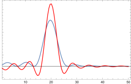
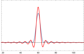
Figure 4: The exact (red) and approximate (blue) profiles of $(zz^{\prime})^{\frac{d-1}{2}}{\rm Im}\Pi(z,z^{\prime})$ as a function of $pz$, taking $pz^{\prime}=20$ (left) and $pz^{\prime}=60$ (right), and taking $d=4$.

Appendix F Bubble Diagrams

In these calculations, we consider bubbles formed of $\lambda\Phi\Phi_{1}\Phi_{2}$ and $\xi\Phi\partial_{M}\Phi_{1}\partial^{M}\Phi_{2}$ vertices, hence the fields and propagators are not treated as identical. We use standard manipulations (Feynman parameterization, dimensional regularization) to evaluate the loop. We define $\Delta=-x(1-x)p^{2}+xm_{1}^{2}+(1-x)m^{2}_{2}$.

When taking the imaginary part of $\Pi$, we use the kinematic approximation of Sec. 5.3 to obtain

$${\rm Im}\int_{x_{-}}^{x_{+}}\log\Delta=-\pi$$ (266)

$${\rm Im}\int_{x_{-}}^{x_{+}}x\log\Delta={\rm Im}\int_{x_{-}}^{x_{+}}(1-x)\log\Delta=-\frac{\pi}{2}$$ (267)

$${\rm Im}\int_{x_{-}}^{x_{+}}x(1-x)\log\Delta=-\frac{\pi}{6}$$ (268)

$${\rm Im}\int_{x_{-}}^{x_{+}}x^{2}(1-x)\log\Delta={\rm Im}\int_{x_{-}}^{x_{+}}x(1-x)^{2}\log\Delta=-\frac{\pi}{12}$$ (269)

$${\rm Im}\int_{x_{-}}^{x_{+}}x^{2}(1-x)^{2}\log\Delta=-\frac{\pi}{30}\,.$$ (270)

$\Phi^{3}-\Phi^{3}$

The amplitude of the bubble induced by two $\lambda\Phi\Phi_{1}\Phi_{2}$ vertices is

$$i\Pi_{\lambda\lambda}(z_{1},z_{2})=\lambda^{2}\frac{1}{k^{4}z_{1}z_{2}}\int dq_{1}dq_{2}q_{1}q_{2}\int\frac{d^{4}q}{(2\pi)^{4}}\frac{J_{\alpha_{1}}(q_{1}z_{1})J_{\alpha_{1}}(q_{1}z_{2})J_{\alpha_{2}}(q_{2}z_{1})J_{\alpha_{2}}(q_{2}z_{2})}{(q^{2}-q^{2}_{1})((q+p)^{2}-q^{2}_{2})}\,.$$ (271)

We introduce a Feynman parameter $x$ and use dimensional regularization to evaluate the loop. We have

$$i\Pi_{\lambda\lambda}(z_{1},z_{2})=$$ (272)

$$\lambda^{2}\frac{1}{k^{4}z_{1}z_{2}}\int dq_{1}dq_{2}q_{1}q_{2}\int^{1}_{0}dx\frac{-i}{16\pi^{2}}\log\left(\frac{\Delta}{\Lambda^{2}}\right)J_{\alpha_{1}}(q_{1}z_{1})J_{\alpha_{1}}(q_{1}z_{2})J_{\alpha_{2}}(q_{2}z_{1})J_{\alpha_{2}}(q_{2}z_{2})+\ldots$$

$\Lambda$ is the regularization scale and the ellipses represent the divergent part of the loop diagram. Both the divergence and the $\Lambda$-dependence vanish upon taking the imaginary part of $\Pi$. Taking the imaginary part gives Eq. (153).

$\Phi^{3}-\Phi(\partial\Phi)^{2}$

The amplitude of the bubble induced by one $\lambda\Phi\Phi_{1}\Phi_{2}$ and one $\xi\Phi\partial_{M}\Phi_{1}\partial^{M}\Phi_{2}$ vertex is given by

$$i\Pi_{\lambda\zeta}(z_{1},z_{2})=$$ (273)

$$-\lambda\zeta\frac{(kz_{2})^{2}}{k^{4}z_{1}z_{2}}\int dq_{1}dq_{2}q_{1}q_{2}\int\frac{d^{4}q}{(2\pi)^{4}}\bigg{(}q.(p+q)-\partial^{(1)}_{z_{2}}\partial^{(2)}_{z_{2}}\bigg{)}\frac{J_{\alpha_{1}}(q_{1}z_{1})J_{\alpha_{1}}(q_{1}z_{2})J_{\alpha_{2}}(q_{2}z_{1})J_{\alpha_{2}}(q_{2}z_{2})}{(q^{2}-q^{2}_{1})((q+p)^{2}-q^{2}_{2})}\,$$

plus its $(1\leftrightarrow 2)$ counterpart. The $\partial_{z}^{(i)}$ derivative acts only on the $G_{q_{i}}(z_{1},z_{2})$ propagator, i.e. only on the $J_{\alpha_{i}}(q_{i}z)$ Bessel function in the above expression and subsequent ones. We introduce a Feynman parameter $x$ and perform the loop integral via dimensional regularization. We obtain

$$i\Pi_{\lambda\zeta} (z_{1},z_{2})=-\lambda\zeta\frac{z_{2}^{2}}{k^{2}z_{1}z_{2}}\int dq_{1}dq_{2}q_{1}q_{2}\int^{1}_{0}dx$$ (274)

$$\frac{-i}{16\pi^{2}}\log\left(\frac{\Delta}{\Lambda^{2}}\right)\bigg{(}2\Delta-x(1-x)p^{2}-\partial^{(1)}_{z_{2}}\partial^{(2)}_{z_{2}}\bigg{)}J_{\alpha_{1}}(q_{1}z_{1})J_{\alpha_{1}}(q_{1}z_{2})J_{\alpha_{2}}(q_{2}z_{1})J_{\alpha_{2}}(q_{2}z_{2})+\ldots$$

$\Lambda$ is the regularization scale and the ellipses represent the divergent part of the loop diagram. Both vanish upon taking the imaginary part of $\Pi$. Taking the imaginary part and including the $(1\leftrightarrow 2)$ contribution gives Eq. (157).

$\Phi(\partial\Phi)^{2}-\Phi(\partial\Phi)^{2}$

The amplitude of the bubble induced by two $\xi\Phi\partial_{M}\Phi_{1}\partial^{M}\Phi_{2}$ vertices is

$$i\Pi_{\zeta\zeta} (z_{1},z_{2})=\zeta^{2}\frac{(kz_{1})^{2}(kz_{2})^{2}}{k^{4}z_{1}z_{2}}\int dq_{1}dq_{2}q_{1}q_{2}\int\frac{d^{4}q}{(2\pi)^{4}}$$ (275)

$$\bigg{(}q.(p+q)-\partial^{(1)}_{z_{1}}\partial^{(2)}_{z_{1}}\bigg{)}\bigg{(}q.(p+q)-\partial^{(1)}_{z_{2}}\partial^{(2)}_{z_{2}}\bigg{)}\frac{J_{\alpha_{1}}(q_{1}z_{1})J_{\alpha_{1}}(q_{1}z_{2})J_{\alpha_{2}}(q_{2}z_{1})J_{\alpha_{2}}(q_{2}z_{2})}{(q^{2}-q^{2}_{1})((q+p)^{2}-q^{2}_{2})}\,.$$

We introduce a Feynman parameter $x$ and perform the loop integral via dimensional regularization to obtain

$$i\Pi_{\zeta\zeta}(z_{1},z_{2})=\zeta^{2}\frac{z_{1}^{2}z_{2}^{2}}{z_{1}z_{2}} \int dq_{1}dq_{2}q_{1}q_{2}\int^{1}_{0}dx\frac{-i}{16\pi^{2}}\log\left(\frac{\Delta}{\Lambda^{2}}\right)$$ (276)

$$\bigg{(}3\Delta^{2}+\left(\frac{1}{2}-6x(1-x)\right)p^{2}\Delta+x^{2}(1-x)^{2}p^{4}$$

$$\quad\quad-(2\Delta-x(1-x)p^{2})\left(\partial^{(1)}_{z_{1}}\partial^{(2)}_{z_{1}}+\partial^{(1)}_{z_{2}}\partial^{(2)}_{z_{2}}\right)+\partial^{(1)}_{z_{1}}\partial^{(2)}_{z_{1}}\partial^{(1)}_{z_{2}}\partial^{(2)}_{z_{2}}\bigg{)}$$

$$\quad\quad\quad\quad\quad\quad\quad\quad\quad\quad\quad\quad J_{\alpha_{1}}(q_{1}z_{1})J_{\alpha_{1}}(q_{1}z_{2})J_{\alpha_{2}}(q_{2}z_{1})J_{\alpha_{2}}(q_{2}z_{2})+\ldots$$

$\Lambda$ is the regularization scale and the ellipses represent the divergent part of the loop diagram. Evaluating the $x$ integrals and taking the imaginary part of $\Pi$ gives

$${\rm Im}\Pi_{\zeta\zeta}(z_{1},z_{2})=\zeta^{2}\frac{z_{1}^{2}z_{2}^{2}}{z_{1}z_{2}}\frac{1}{16\pi} \int dq_{1}dq_{2}q_{1}q_{2}$$ (277)

$$\bigg{(}q^{4}_{1}+q^{4}_{2}+q^{2}_{1}q^{2}_{2}-\frac{3}{4}p^{2}(q_{1}^{2}+q_{2}^{2})+\frac{p^{4}}{4}$$

$$\quad\quad-\left(q_{1}^{2}+q_{2}^{2}-\frac{p^{2}}{2}\right)\left(\partial^{(1)}_{z_{1}}\partial^{(2)}_{z_{1}}+\partial^{(1)}_{z_{2}}\partial^{(2)}_{z_{2}}\right)+\partial^{(1)}_{z_{1}}\partial^{(2)}_{z_{1}}\partial^{(1)}_{z_{2}}\partial^{(2)}_{z_{2}}\bigg{)}$$

$$\quad\quad\quad\quad\quad\quad\quad\quad\quad\quad\quad\quad J_{\alpha_{1}}(q_{1}z_{1})J_{\alpha_{1}}(q_{1}z_{2})J_{\alpha_{2}}(q_{2}z_{1})J_{\alpha_{2}}(q_{2}z_{2})\,.$$

Scalar-Graviton Bubble

The amplitude induced by the scalar component of the graviton multiplet is

$$i\Pi^{\phi}(z_{1},z_{2})=\frac{-1}{3\,M_{*}^{3}} \left(\frac{m_{\Phi}^{2}}{2(kz_{1})^{2}}-\frac{3}{2}\partial_{z_{1}}\partial_{z_{1}}^{G_{\Phi}}\right)\left(\frac{m_{\Phi}^{2}}{2(kz_{2})^{2}}-\frac{3}{2}\partial_{z_{2}}\partial_{z_{2}}^{G_{\Phi}}\right)$$ (278)

$$\frac{1}{(kz_{1})(kz_{2})}\int\frac{dq^{4}}{(2\pi)^{4}}G^{\Phi}_{\alpha}(q_{1},z_{1},z_{2})G^{\phi}(q_{2},z_{2},z_{1})\,.$$

The $\partial_{z}^{G_{\Phi}}$ derivatives act only on the internal $\Phi$ propagator (henceforth the term contained in square brackets). Introducing the propagators in their momentum spectral representations, we have

$$i\Pi^{\phi}(z_{1},z_{2})=\frac{1}{3\,M_{*}^{3}} \left(\frac{m_{\Phi}^{2}}{2(kz_{1})^{2}}-\frac{3}{2}\partial_{z_{1}}\partial_{z_{1}}^{G_{\Phi}}\right)\left(\frac{m_{\Phi}^{2}}{2(kz_{2})^{2}}-\frac{3}{2}\partial_{z_{2}}\partial_{z_{2}}^{G_{\Phi}}\right)$$ (279)

$$\frac{1}{z_{1}z_{2}}\int dq_{1}dq_{2}q_{1}q_{2}\int\frac{dq^{4}}{(2\pi)^{4}}\frac{\left[z_{1}^{2}z_{2}^{2}J_{\alpha}(q_{1}z_{1})J_{\alpha}(q_{1}z_{2})\right]J_{0}(q_{2}z_{1})J_{0}(q_{2}z_{2})}{(q^{2}-q^{2}_{1})((q+p)^{2}-q^{2}_{2})}\,.$$

We introduce a Feynman parameter and perform the loop integral to obtain

$$i\Pi^{\phi}(z_{1},z_{2})= \frac{-i}{48\pi^{2}\,M_{*}^{3}}\left(\frac{m_{\Phi}^{2}}{2(kz_{1})^{2}}-\frac{3}{2}\partial_{z_{1}}\partial_{z_{1}}^{G_{\Phi}}\right)\left(\frac{m_{\Phi}^{2}}{2(kz_{2})^{2}}-\frac{3}{2}\partial_{z_{2}}\partial_{z_{2}}^{G_{\Phi}}\right)$$ (280)

$$\frac{1}{z_{1}z_{2}}\int dq_{1}dq_{2}q_{1}q_{2}\int^{1}_{0}dx\log\left(\frac{\Delta}{\Lambda^{2}}\right)\left[z_{1}^{2}z_{2}^{2}J_{\alpha}(q_{1}z_{1})J_{\alpha}(q_{1}z_{2})\right]J_{0}(q_{2}z_{1})J_{0}(q_{2}z_{2})\,.$$

Taking the imaginary part gives Eq. (188).

References

- (1) V. Balasubramanian, S. B. Giddings, and A. E. Lawrence, What do CFTs tell us about Anti-de Sitter space-times?, JHEP 03 (1999) 001, [hep-th/9902052].
- (2) S. B. Giddings, The Boundary S matrix and the AdS to CFT dictionary, Phys. Rev. Lett. 83 (1999) 2707–2710, [hep-th/9903048].
- (3) D. Meltzer, E. Perlmutter, and A. Sivaramakrishnan, Unitarity Methods in AdS/CFT, JHEP 03 (2020) 061, [arXiv:1912.09521].
- (4) I. Heemskerk, J. Penedones, J. Polchinski, and J. Sully, Holography from Conformal Field Theory, JHEP 10 (2009) 079, [arXiv:0907.0151].
- (5) J. Penedones, Writing CFT correlation functions as AdS scattering amplitudes, JHEP 03 (2011) 025, [arXiv:1011.1485].
- (6) L. Cornalba, M. S. Costa, and J. Penedones, Eikonal approximation in AdS/CFT: Resumming the gravitational loop expansion, JHEP 09 (2007) 037, [arXiv:0707.0120].
- (7) A. Fitzpatrick and J. Kaplan, Analyticity and the Holographic S-Matrix, JHEP 10 (2012) 127, [arXiv:1111.6972].
- (8) L. F. Alday and A. Bissi, Loop Corrections to Supergravity on , Phys. Rev. Lett. 119 (2017), no. 17 171601, [arXiv:1706.02388].
- (9) L. F. Alday and S. Caron-Huot, Gravitational S-matrix from CFT dispersion relations, JHEP 12 (2018) 017, [arXiv:1711.02031].
- (10) L. F. Alday, A. Bissi, and E. Perlmutter, Genus-One String Amplitudes from Conformal Field Theory, JHEP 06 (2019) 010, [arXiv:1809.10670].
- (11) L. F. Alday, On Genus-one String Amplitudes on , arXiv:1812.11783.
- (12) D. Meltzer, Higher Spin ANEC and the Space of CFTs, JHEP 07 (2019) 001, [arXiv:1811.01913].
- (13) D. Ponomarev, E. Sezgin, and E. Skvortsov, On one loop corrections in higher spin gravity, JHEP 11 (2019) 138, [arXiv:1904.01042].
- (14) M. Shyani, Lorentzian inversion and anomalous dimensions in Mellin space, arXiv:1908.00015.
- (15) L. F. Alday and E. Perlmutter, Growing Extra Dimensions in AdS/CFT, JHEP 08 (2019) 084, [arXiv:1906.01477].
- (16) L. F. Alday and X. Zhou, Simplicity of AdS Supergravity at One Loop, arXiv:1912.02663.
- (17) D. Meltzer, AdS/CFT Unitarity at Higher Loops: High-Energy String Scattering, JHEP 05 (2020) 133, [arXiv:1912.05580].
- (18) F. Aprile, J. Drummond, P. Heslop, and H. Paul, Quantum Gravity from Conformal Field Theory, JHEP 01 (2018) 035, [arXiv:1706.02822].
- (19) F. Aprile, J. Drummond, P. Heslop, and H. Paul, Unmixing Supergravity, JHEP 02 (2018) 133, [arXiv:1706.08456].
- (20) F. Aprile, J. Drummond, P. Heslop, and H. Paul, Loop corrections for Kaluza-Klein AdS amplitudes, JHEP 05 (2018) 056, [arXiv:1711.03903].
- (21) S. Giombi, C. Sleight, and M. Taronna, Spinning AdS Loop Diagrams: Two Point Functions, JHEP 06 (2018) 030, [arXiv:1708.08404].
- (22) C. Cardona, Mellin-(Schwinger) representation of One-loop Witten diagrams in AdS, arXiv:1708.06339.
- (23) O. Aharony, L. F. Alday, A. Bissi, and E. Perlmutter, Loops in AdS from Conformal Field Theory, JHEP 07 (2017) 036, [arXiv:1612.03891].
- (24) E. Y. Yuan, Loops in the Bulk, arXiv:1710.01361.
- (25) E. Y. Yuan, Simplicity in AdS Perturbative Dynamics, arXiv:1801.07283.
- (26) I. Bertan, I. Sachs, and E. D. Skvortsov, Quantum Theory in AdS4 and its CFT Dual, JHEP 02 (2019) 099, [arXiv:1810.00907].
- (27) I. Bertan and I. Sachs, Loops in Anti–de Sitter Space, Phys. Rev. Lett. 121 (2018), no. 10 101601, [arXiv:1804.01880].
- (28) J. Liu, E. Perlmutter, V. Rosenhaus, and D. Simmons-Duffin, -dimensional SYK, AdS Loops, and Symbols, JHEP 03 (2019) 052, [arXiv:1808.00612].
- (29) D. Carmi, L. Di Pietro, and S. Komatsu, A Study of Quantum Field Theories in AdS at Finite Coupling, JHEP 01 (2019) 200, [arXiv:1810.04185].
- (30) F. Aprile, J. Drummond, P. Heslop, and H. Paul, Double-trace spectrum of supersymmetric Yang-Mills theory at strong coupling, Phys. Rev. D 98 (2018), no. 12 126008, [arXiv:1802.06889].
- (31) K. Ghosh, Polyakov-Mellin Bootstrap for AdS loops, JHEP 02 (2020) 006, [arXiv:1811.00504].
- (32) D. Mazac and M. F. Paulos, The analytic functional bootstrap. Part II. Natural bases for the crossing equation, JHEP 02 (2019) 163, [arXiv:1811.10646].
- (33) M. Beccaria and A. A. Tseytlin, On boundary correlators in Liouville theory on AdS2, JHEP 07 (2019) 008, [arXiv:1904.12753].
- (34) S. M. Chester, Genus-2 holographic correlator on AdS S5 from localization, JHEP 04 (2020) 193, [arXiv:1908.05247].
- (35) M. Beccaria, H. Jiang, and A. A. Tseytlin, Supersymmetric Liouville theory in AdS2 and AdS/CFT, JHEP 11 (2019) 051, [arXiv:1909.10255].
- (36) D. Carmi, Loops in AdS: From the Spectral Representation to Position Space, arXiv:1910.14340.
- (37) F. Aprile, J. Drummond, P. Heslop, and H. Paul, One-loop amplitudes in AdS S5 supergravity from = 4 SYM at strong coupling, JHEP 03 (2020) 190, [arXiv:1912.01047].
- (38) S. Fichet, Opacity and effective field theory in anti–de Sitter backgrounds, Phys. Rev. D100 (2019), no. 9 095002, [arXiv:1905.05779].
- (39) J. Drummond and H. Paul, One-loop string corrections to AdS amplitudes from CFT, arXiv:1912.07632.
- (40) S. Albayrak, C. Chowdhury, and S. Kharel, An étude of momentum space scalar amplitudes in AdS, arXiv:2001.06777.
- (41) S. Albayrak and S. Kharel, On spinning loop amplitudes in Anti-de Sitter space, arXiv:2006.12540.
- (42) D. Meltzer and A. Sivaramakrishnan, CFT Unitarity and the AdS Cutkosky Rules, arXiv:2008.11730.
- (43) S. Raju, BCFW for Witten Diagrams, Phys. Rev. Lett. 106 (2011) 091601, [arXiv:1011.0780].
- (44) S. Raju, Four Point Functions of the Stress Tensor and Conserved Currents in AdS4/CFT3, Phys. Rev. D 85 (2012) 126008, [arXiv:1201.6452].
- (45) S. Raju, New Recursion Relations and a Flat Space Limit for AdS/CFT Correlators, Phys. Rev. D 85 (2012) 126009, [arXiv:1201.6449].
- (46) S. Raju, Recursion Relations for AdS/CFT Correlators, Phys. Rev. D 83 (2011) 126002, [arXiv:1102.4724].
- (47) A. Bzowski, P. McFadden, and K. Skenderis, Implications of conformal invariance in momentum space, JHEP 03 (2014) 111, [arXiv:1304.7760].
- (48) A. Bzowski, P. McFadden, and K. Skenderis, Scalar 3-point functions in CFT: renormalisation, beta functions and anomalies, JHEP 03 (2016) 066, [arXiv:1510.08442].
- (49) A. Bzowski, P. McFadden, and K. Skenderis, Renormalised CFT 3-point functions of scalars, currents and stress tensors, JHEP 11 (2018) 159, [arXiv:1805.12100].
- (50) A. Bzowski, P. McFadden, and K. Skenderis, Evaluation of conformal integrals, JHEP 02 (2016) 068, [arXiv:1511.02357].
- (51) H. Isono, T. Noumi, and T. Takeuchi, Momentum space conformal three-point functions of conserved currents and a general spinning operator, JHEP 05 (2019) 057, [arXiv:1903.01110].
- (52) H. Isono, T. Noumi, and G. Shiu, Momentum space approach to crossing symmetric CFT correlators, JHEP 07 (2018) 136, [arXiv:1805.11107].
- (53) H. Isono, T. Noumi, and G. Shiu, Momentum space approach to crossing symmetric CFT correlators. Part II. General spacetime dimension, JHEP 10 (2019) 183, [arXiv:1908.04572].
- (54) C. Corianò and M. M. Maglio, Exact Correlators from Conformal Ward Identities in Momentum Space and the Perturbative Vertex, Nucl. Phys. B 938 (2019) 440–522, [arXiv:1802.07675].
- (55) C. Corianò, M. M. Maglio, A. Tatullo, and D. Theofilopoulos, Exact Correlators from Conformal Ward Identities in Momentum Space and Perturbative Realizations, PoS CORFU2018 (2019) 072, [arXiv:1904.13174].
- (56) C. Corianò and M. M. Maglio, On Some Hypergeometric Solutions of the Conformal Ward Identities of Scalar 4-point Functions in Momentum Space, JHEP 09 (2019) 107, [arXiv:1903.05047].
- (57) M. Gillioz, Momentum-space conformal blocks on the light cone, JHEP 10 (2018) 125, [arXiv:1807.07003].
- (58) C. Coriano, L. Delle Rose, E. Mottola, and M. Serino, Solving the Conformal Constraints for Scalar Operators in Momentum Space and the Evaluation of Feynman’s Master Integrals, JHEP 07 (2013) 011, [arXiv:1304.6944].
- (59) A. Bzowski, P. McFadden, and K. Skenderis, Conformal -point functions in momentum space, Phys. Rev. Lett. 124 (2020), no. 13 131602, [arXiv:1910.10162].
- (60) M. Gillioz, Conformal 3-point functions and the Lorentzian OPE in momentum space, arXiv:1909.00878.
- (61) J. A. Farrow, A. E. Lipstein, and P. McFadden, Double copy structure of CFT correlators, JHEP 02 (2019) 130, [arXiv:1812.11129].
- (62) B. Nagaraj and D. Ponomarev, Spinor-helicity formalism for massless fields in AdS4. Part II. Potentials, JHEP 06 (2020) 068, [arXiv:1912.07494].
- (63) S. Albayrak and S. Kharel, Towards the higher point holographic momentum space amplitudes, JHEP 02 (2019) 040, [arXiv:1810.12459].
- (64) S. Albayrak and S. Kharel, Towards the higher point holographic momentum space amplitudes. Part II. Gravitons, JHEP 12 (2019) 135, [arXiv:1908.01835].
- (65) S. Albayrak, C. Chowdhury, and S. Kharel, New relation for Witten diagrams, JHEP 10 (2019) 274, [arXiv:1904.10043].
- (66) J. M. Maldacena, Non-Gaussian features of primordial fluctuations in single field inflationary models, JHEP 05 (2003) 013, [astro-ph/0210603].
- (67) J. M. Maldacena and G. L. Pimentel, On graviton non-Gaussianities during inflation, JHEP 09 (2011) 045, [arXiv:1104.2846].
- (68) I. Mata, S. Raju, and S. Trivedi, CMB from CFT, JHEP 07 (2013) 015, [arXiv:1211.5482].
- (69) N. Kundu, A. Shukla, and S. P. Trivedi, Constraints from Conformal Symmetry on the Three Point Scalar Correlator in Inflation, JHEP 04 (2015) 061, [arXiv:1410.2606].
- (70) A. Ghosh, N. Kundu, S. Raju, and S. P. Trivedi, Conformal Invariance and the Four Point Scalar Correlator in Slow-Roll Inflation, JHEP 07 (2014) 011, [arXiv:1401.1426].
- (71) N. Arkani-Hamed and J. Maldacena, Cosmological Collider Physics, arXiv:1503.08043.
- (72) N. Kundu, A. Shukla, and S. P. Trivedi, Ward Identities for Scale and Special Conformal Transformations in Inflation, JHEP 01 (2016) 046, [arXiv:1507.06017].
- (73) C. Sleight, A Mellin Space Approach to Cosmological Correlators, JHEP 01 (2020) 090, [arXiv:1906.12302].
- (74) C. Sleight and M. Taronna, Bootstrapping Inflationary Correlators in Mellin Space, JHEP 02 (2020) 098, [arXiv:1907.01143].
- (75) C. Sleight and M. Taronna, From AdS to dS Exchanges: Spectral Representation, Mellin Amplitudes and Crossing, arXiv:2007.09993.
- (76) N. Arkani-Hamed, P. Benincasa, and A. Postnikov, Cosmological Polytopes and the Wavefunction of the Universe, arXiv:1709.02813.
- (77) N. Arkani-Hamed and P. Benincasa, On the Emergence of Lorentz Invariance and Unitarity from the Scattering Facet of Cosmological Polytopes, arXiv:1811.01125.
- (78) P. Benincasa, From the flat-space S-matrix to the Wavefunction of the Universe, arXiv:1811.02515.
- (79) P. Benincasa, Cosmological Polytopes and the Wavefuncton of the Universe for Light States, arXiv:1909.02517.
- (80) N. Arkani-Hamed, D. Baumann, H. Lee, and G. L. Pimentel, The Cosmological Bootstrap: Inflationary Correlators from Symmetries and Singularities, JHEP 04 (2020) 105, [arXiv:1811.00024].
- (81) D. Baumann, C. Duaso Pueyo, A. Joyce, H. Lee, and G. L. Pimentel, The Cosmological Bootstrap: Weight-Shifting Operators and Scalar Seeds, arXiv:1910.14051.
- (82) D. Baumann, C. Duaso Pueyo, A. Joyce, H. Lee, and G. L. Pimentel, The Cosmological Bootstrap: Spinning Correlators from Symmetries and Factorization, arXiv:2005.04234.
- (83) N. Arkani-Hamed, M. Porrati, and L. Randall, Holography and phenomenology, JHEP 08 (2001) 017, [hep-th/0012148].
- (84) A. Costantino, S. Fichet, and P. Tanedo, Effective Field Theory in AdS: Continuum Regime, Soft Bombs, and IR Emergence, arXiv:2002.12335.
- (85) J. Callan, Curtis G. and F. Wilczek, INFRARED BEHAVIOR AT NEGATIVE CURVATURE, Nucl. Phys. B 340 (1990) 366–386.
- (86) D. McAvity and H. Osborn, Conformal field theories near a boundary in general dimensions, Nucl. Phys. B 455 (1995) 522–576, [cond-mat/9505127].
- (87) S. Giombi and H. Khanchandani, CFT in AdS and boundary RG flows, arXiv:2007.04955.
- (88) J. M. Maldacena, The Large N limit of superconformal field theories and supergravity, Int. J. Theor. Phys. 38 (1999) 1113–1133, [hep-th/9711200]. [Adv. Theor. Math. Phys.2,231(1998)].
- (89) S. S. Gubser, I. R. Klebanov, and A. M. Polyakov, Gauge theory correlators from noncritical string theory, Phys. Lett. B428 (1998) 105–114, [hep-th/9802109].
- (90) E. Witten, Anti-de Sitter space and holography, Adv. Theor. Math. Phys. 2 (1998) 253–291, [hep-th/9802150].
- (91) D. Z. Freedman, S. D. Mathur, A. Matusis, and L. Rastelli, Comments on 4 point functions in the CFT / AdS correspondence, Phys. Lett. B 452 (1999) 61–68, [hep-th/9808006].
- (92) H. Liu and A. A. Tseytlin, On four point functions in the CFT / AdS correspondence, Phys. Rev. D 59 (1999) 086002, [hep-th/9807097].
- (93) D. Z. Freedman, S. D. Mathur, A. Matusis, and L. Rastelli, Correlation functions in the CFT(d) / AdS(d+1) correspondence, Nucl. Phys. B 546 (1999) 96–118, [hep-th/9804058].
- (94) E. D’Hoker, D. Z. Freedman, and L. Rastelli, AdS / CFT four point functions: How to succeed at z integrals without really trying, Nucl. Phys. B 562 (1999) 395–411, [hep-th/9905049].
- (95) E. D’Hoker, D. Z. Freedman, S. D. Mathur, A. Matusis, and L. Rastelli, Graviton exchange and complete four point functions in the AdS / CFT correspondence, Nucl. Phys. B 562 (1999) 353–394, [hep-th/9903196].
- (96) O. Aharony, S. S. Gubser, J. M. Maldacena, H. Ooguri, and Y. Oz, Large N field theories, string theory and gravity, Phys. Rept. 323 (2000) 183–386, [hep-th/9905111].
- (97) A. Zaffaroni, Introduction to the AdS-CFT correspondence, Class. Quant. Grav. 17 (2000) 3571–3597.
- (98) H. Nastase, Introduction to AdS-CFT, arXiv:0712.0689.
- (99) J. Kaplan, “Lectures on AdS/CFT from the Bottom Up.” https://sites.krieger.jhu.edu/jared-kaplan/files/2016/05/AdSCFTCourseNotesCurrentPublic.pdf.
- (100) L. Randall and R. Sundrum, A Large mass hierarchy from a small extra dimension, Phys. Rev. Lett. 83 (1999) 3370–3373, [hep-ph/9905221].
- (101) L. Randall and R. Sundrum, An Alternative to compactification, Phys. Rev. Lett. 83 (1999) 4690–4693, [hep-th/9906064].
- (102) P. Brax and C. van de Bruck, Cosmology and brane worlds: A Review, Class. Quant. Grav. 20 (2003) R201–R232, [hep-th/0303095].
- (103) B. von Harling and K. L. McDonald, Secluded Dark Matter Coupled to a Hidden CFT, JHEP 08 (2012) 048, [arXiv:1203.6646].
- (104) K. L. McDonald and D. E. Morrissey, Low-Energy Signals from Kinetic Mixing with a Warped Abelian Hidden Sector, JHEP 02 (2011) 087, [arXiv:1010.5999].
- (105) K. L. McDonald and D. E. Morrissey, Low-Energy Probes of a Warped Extra Dimension, JHEP 05 (2010) 056, [arXiv:1002.3361].
- (106) P. Brax, S. Fichet, and P. Tanedo, The Warped Dark Sector, Phys. Lett. B798 (2019) 135012, [arXiv:1906.02199].
- (107) S. Caron-Huot, Analyticity in Spin in Conformal Theories, JHEP 09 (2017) 078, [arXiv:1703.00278].
- (108) D. W. Dusedau and D. Z. Freedman, Lehmann Spectral Representation for Anti-de Sitter Quantum Field Theory, Phys. Rev. D 33 (1986) 389.
- (109) C. J. Burges, D. Z. Freedman, S. Davis, and G. Gibbons, Supersymmetry in Anti-de Sitter Space, Annals Phys. 167 (1986) 285.
- (110) S. Fichet, Braneworld effective field theories — holography, consistency and conformal effects, JHEP 04 (2020) 016, [arXiv:1912.12316].
- (111) T. Leonhardt, R. Manvelyan, and W. Ruhl, The Group approach to AdS space propagators, Nucl. Phys. B 667 (2003) 413–434, [hep-th/0305235].
- (112) “NIST Digital Library of Mathematical Functions.” http://dlmf.nist.gov/, Release 1.0.28 of 2020-09-15. F. W. J. Olver, A. B. Olde Daalhuis, D. W. Lozier, B. I. Schneider, R. F. Boisvert, C. W. Clark, B. R. Miller, B. V. Saunders, H. S. Cohl, and M. A. McClain, eds.
- (113) R. Zwicky, A brief Introduction to Dispersion Relations and Analyticity, in Quantum Field Theory at the Limits: from Strong Fields to Heavy Quarks, pp. 93–120, 2017. arXiv:1610.06090.
- (114) M. E. Peskin and D. V. Schroeder, An introduction to quantum field theory. Westview, Boulder, CO, 1995.
- (115) N. Birrell and P. Davies, Quantum Fields in Curved Space. Cambridge Monographs on Mathematical Physics. Cambridge University Press, 1984.
- (116) M. F. Paulos, Towards Feynman rules for Mellin amplitudes, JHEP 10 (2011) 074, [arXiv:1107.1504].
- (117) G. Mack, D-dimensional Conformal Field Theories with anomalous dimensions as Dual Resonance Models, Bulg. J. Phys. 36 (2009) 214–226, [arXiv:0909.1024].
- (118) S. Kharel and G. Siopsis, Tree-level Correlators of scalar and vector fields in AdS/CFT, JHEP 11 (2013) 159, [arXiv:1308.2515].
- (119) A. Fitzpatrick and J. Kaplan, Unitarity and the Holographic S-Matrix, JHEP 10 (2012) 032, [arXiv:1112.4845].
- (120) M. S. Costa, V. Gonçalves, and J. Penedones, Spinning AdS Propagators, JHEP 09 (2014) 064, [arXiv:1404.5625].
- (121) M. F. Paulos, J. Penedones, J. Toledo, B. C. van Rees, and P. Vieira, The S-matrix bootstrap. Part I: QFT in AdS, JHEP 11 (2017) 133, [arXiv:1607.06109].
- (122) C. B. Jepsen and S. Parikh, Recursion Relations in -adic Mellin Space, J. Phys. A 52 (2019), no. 28 285401, [arXiv:1812.09801].
- (123) C. B. Jepsen and S. Parikh, -adic Mellin Amplitudes, JHEP 04 (2019) 101, [arXiv:1808.08333].
- (124) S. S. Gubser, C. Jepsen, and B. Trundy, Spin in -adic AdS/CFT, J. Phys. A 52 (2019), no. 14 144004, [arXiv:1811.02538].
- (125) E. Hijano, P. Kraus, E. Perlmutter, and R. Snively, Witten Diagrams Revisited: The AdS Geometry of Conformal Blocks, JHEP 01 (2016) 146, [arXiv:1508.00501].
- (126) S. Parikh, Holographic dual of the five-point conformal block, JHEP 05 (2019) 051, [arXiv:1901.01267].
- (127) C. B. Jepsen and S. Parikh, Propagator identities, holographic conformal blocks, and higher-point AdS diagrams, JHEP 10 (2019) 268, [arXiv:1906.08405].
- (128) J. Penedones, J. A. Silva, and A. Zhiboedov, Nonperturbative Mellin Amplitudes: Existence, Properties, Applications, JHEP 08 (2020) 031, [arXiv:1912.11100].
- (129) D. Ponomarev, From bulk loops to boundary large-N expansion, JHEP 01 (2020) 154, [arXiv:1908.03974].
- (130) S. Caron-Huot and A.-K. Trinh, All tree-level correlators in AdSS5 supergravity: hidden ten-dimensional conformal symmetry, JHEP 01 (2019) 196, [arXiv:1809.09173].
- (131) A. Fitzpatrick, J. Kaplan, J. Penedones, S. Raju, and B. C. van Rees, A Natural Language for AdS/CFT Correlators, JHEP 11 (2011) 095, [arXiv:1107.1499].
- (132) S. Fichet, B. Jain, E. Ponton, M. Quiros, and R. Rosenfeld, “Private Communication.”
- (133) W. R. Inc., “Mathematica, Version 12.1.” https://www.wolfram.com/mathematica. Champaign, IL, 2020.
- (134) W. D. Goldberger and I. Z. Rothstein, High-energy field theory in truncated AdS backgrounds, Phys. Rev. Lett. 89 (2002) 131601, [hep-th/0204160].
- (135) W. D. Goldberger and I. Z. Rothstein, Effective field theory and unification in AdS backgrounds, Phys. Rev. D68 (2003) 125011, [hep-th/0208060].
- (136) E. Ponton, TASI 2011: Four Lectures on TeV Scale Extra Dimensions, in Theoretical Advanced Study Institute in Elementary Particle Physics: The Dark Secrets of the Terascale, pp. 283–374, 2013. arXiv:1207.3827.
- (137) Z. Chacko, M. A. Luty, and E. Ponton, Massive higher dimensional gauge fields as messengers of supersymmetry breaking, JHEP 07 (2000) 036, [hep-ph/9909248].
- (138) K. Agashe, H. Davoudiasl, G. Perez, and A. Soni, Warped Gravitons at the LHC and Beyond, Phys. Rev. D76 (2007) 036006, [hep-ph/0701186].
- (139) A. Karch, E. Katz, D. T. Son, and M. A. Stephanov, Linear confinement and AdS/QCD, Phys. Rev. D74 (2006) 015005, [hep-ph/0602229].
- (140) U. Gursoy and E. Kiritsis, Exploring improved holographic theories for QCD: Part I, JHEP 02 (2008) 032, [arXiv:0707.1324].
- (141) U. Gursoy, E. Kiritsis, and F. Nitti, Exploring improved holographic theories for QCD: Part II, JHEP 02 (2008) 019, [arXiv:0707.1349].
- (142) S. S. Gubser and A. Nellore, Mimicking the QCD equation of state with a dual black hole, Phys. Rev. D 78 (2008) 086007, [arXiv:0804.0434].
- (143) A. Falkowski and M. Perez-Victoria, Electroweak Breaking on a Soft Wall, JHEP 12 (2008) 107, [arXiv:0806.1737].
- (144) B. Batell and T. Gherghetta, Dynamical Soft-Wall AdS/QCD, Phys. Rev. D78 (2008) 026002, [arXiv:0801.4383].
- (145) B. Batell, T. Gherghetta, and D. Sword, The Soft-Wall Standard Model, Phys. Rev. D78 (2008) 116011, [arXiv:0808.3977].
- (146) J. A. Cabrer, G. von Gersdorff, and M. Quiros, Soft-Wall Stabilization, New J. Phys. 12 (2010) 075012, [arXiv:0907.5361].
- (147) G. von Gersdorff, From Soft Walls to Infrared Branes, Phys. Rev. D82 (2010) 086010, [arXiv:1005.5134].
- (148) J. A. Cabrer, G. von Gersdorff, and M. Quiros, Suppressing Electroweak Precision Observables in 5D Warped Models, JHEP 05 (2011) 083, [arXiv:1103.1388].
- (149) K. L. McDonald, Sommerfeld Enhancement from Multiple Mediators, JHEP 07 (2012) 145, [arXiv:1203.6341].
- (150) A. Costantino, S. Fichet, and P. Tanedo, Exotic Spin-Dependent Forces from a Hidden Sector, arXiv:1910.02972. To appear in JHEP.
- (151) D. Z. Freedman, S. S. Gubser, K. Pilch, and N. P. Warner, Renormalization group flows from holography supersymmetry and a c theorem, Adv. Theor. Math. Phys. 3 (1999) 363–417, [hep-th/9904017].
- (152) E. Dudas and G. von Gersdorff, Universal contributions to scalar masses from five dimensional supergravity, JHEP 10 (2012) 100, [arXiv:1207.0815].
- (153) E. E. Boos, Y. A. Kubyshin, M. N. Smolyakov, and I. P. Volobuev, Effective Lagrangians for physical degrees of freedom in the Randall-Sundrum model, Class. Quant. Grav. 19 (2002) 4591–4606, [hep-th/0202009].
- (154) K. Hinterbichler, Theoretical Aspects of Massive Gravity, Rev. Mod. Phys. 84 (2012) 671–710, [arXiv:1105.3735].
- (155) J. Polchinski and M. J. Strassler, Deep inelastic scattering and gauge / string duality, JHEP 05 (2003) 012, [hep-th/0209211].
- (156) D. Karateev, P. Kravchuk, and D. Simmons-Duffin, Harmonic Analysis and Mean Field Theory, JHEP 10 (2019) 217, [arXiv:1809.05111].