Gaussian Transforms Modeling and the Estimation of Distributional Regression Functions

Abstract.

Conditional distribution functions are important statistical objects for the analysis of a wide class of problems in econometrics and statistics. We propose flexible Gaussian representations for conditional distribution functions and give a concave likelihood formulation for their global estimation. We obtain solutions that satisfy the monotonicity property of conditional distribution functions, including under general misspecification and in finite samples. A Lasso-type penalized version of the corresponding maximum likelihood estimator is given that expands the scope of our estimation analysis to models with sparsity. Inference and estimation results for conditional distribution, quantile and density functions implied by our representations are provided and illustrated with an empirical example and simulations.

1. Introduction

The modeling and estimation of conditional distribution functions are important for the analysis of various econometric and statistical problems. Conditional distribution functions are core building blocks in the identification and estimation of nonseparable models with endogeneity (e.g., Imbens and Newey, 2009; Chernozhukov, Fernandez-Val, Newey, Stouli, and Vella, 2020), in counterfactual distributional analysis (e.g., DiNardo, Fortin, and Lemieux, 1996; Chernozhukov, Fernandez-Val, and Melly, 2013), or in the construction of prediction intervals for a stationary time series (e.g., Hall, Wolff, and Yao, 1999; Chernozhukov, Wutrich, and Zhu, 2019). Conditional distribution functions are also a fruitful starting point for the formulation of flexible estimation methods for other objects of interest (Spady and Stouli, 2018a), such as conditional quantile functions (CQF).

For a continuous outcome variable $Y$ and a vector of covariates $X$, three main difficulties arise in the formulation of a flexible model and in the choice of a loss function for the estimation of the conditional distribution and quantile functions of $Y$ given $X$. A first main difficulty is the specification of a model that allows for the shape of the distribution of $Y$ to vary across values of $X$, while being characterized by a loss function that preserves monotonicity in $Y$ at each value of a potentially large number of explanatory variables $X$ in estimation. Because a valid maximum likelihood (ML) characterization would require this monotonicity property to hold, a second and related difficulty is the formulation of a loss function that characterizes an approximate model with a clear information-theoretic interpretation under misspecification. A third difficulty is that nonconcave likelihoods naturally arise in the context of nonseparable models, even in the simplest case of a Gaussian location-scale specification.

One approach is to discard the monotonicity requirement in estimation and use loss functions that characterize quantile or distribution functions pointwise, while specifying a functional form that allows for the shape of the distribution of $Y$ to vary across values of $X$. Quantile regression (Koenker and Basset, 1978) specifies each CQF as a linear combination of the components of $X$. The CQF is then estimated at each quantile by a sequence of linear programming problems. Distribution regression (Foresi and Perrachi, 1995; Chernozhukov, Fernandez-Val, and Melly, 2013) specifies each level of the cumulative distribution function (CDF) of $Y$ conditional on $X$ as a known CDF transformation of a linear combination of the components of $X$. The conditional CDF is then estimated at each $Y$ value by a sequence of binary outcome ML estimators. Another approach is to insist on the monotonicity requirement and use loss functions that characterize both quantile and distribution functions globally, but do not have an ML interpretation. Dual regression (Spady and Stouli, 2018a) specifies monotone representations for $Y$ given $X$ as linear combinations of known functions of $X$ and a stochastic element. The conditional CDF is then estimated globally by the empirical distribution of the estimated sample values of the stochastic element.

In this paper we take a different approach by formulating Gaussian representations for conditional CDFs, instead of modeling conditional CDFs or CQFs directly. These representations are specified as linear combinations of known functions of $X$ and $Y$, and the implied distributional regression models allow for the shape of the distribution of $Y$ to vary across values of $X$. We give a concave likelihood characterization that rules out nonmonotone solutions. Under general misspecification, this formulation also characterizes quasi-Gaussian representations that satisfy the monotonicity property of conditional CDFs by construction. The corresponding distributional models are optimal approximations to the true data probability distribution according to the Kullback-Leibler Information Criterion (KLIC) (White, 1982).

For estimation we derive the properties of the corresponding ML estimator and extend our analysis to a two-step penalized ML estimation strategy, where the unpenalized estimator is used as a first step for an adaptive Lasso (Zou, 2006) ML estimator which preserves the concavity of the objective function. We derive asymptotic properties of the corresponding estimators for conditional distribution, quantile and density functions. The penalized estimator is selection consistent, asymptotically normal and oracle, where the selection is based on the pseudo-true values of the parameter estimators. Under correct specification the estimator is also efficient. We also give the dual formulation of our estimators that we use for implementation.

This paper makes five main contributions to the existing literature. First, we introduce a new class of Gaussian representations in linear form for the flexible estimation of distributional regression models. Second, we demonstrate that our models and the corresponding loss function characterize globally monotone conditional CDFs and CQFs under general misspecification, both in finite samples with probability approaching one and in the population. Quantile and distribution regression can result in both finite sample estimates and population approximations under misspecification that do not satisfy the monotonicity property of conditional quantile and distribution functions. Third, we establish that the resulting approximations are KLIC optimal under general misspecification. Compared to dual regression, we find that the monotonicity property can be obtained jointly with the KLIC optimality property, and we establish existence and uniqueness of solutions under general misspecification. Fourth, we use duality theory to show that our formulation has considerable computational advantages. Compared to dual regression, we find in particular that the dual ML problem has the important advantage of being a convex programming problem (Boyd and Vandenberghe, 2004) with linear constraints. Fifth, our estimation analysis allows for sparsity, thereby giving an asymptotically valid characterization of sparse, globally monotone, and KLIC optimal representations for conditional CDFs and CQFs.

In Section 2 we introduce Gaussian transforms modeling. In Section 3 we give results under misspecification. Section 4 contains estimation and inference results, and duality theory is derived in Section 5. Section 6 illustrates our methods, and Section 7 concludes. The proofs of all results are given in the Appendix. The online Appendix Spady and Stouli (2020) contains supplemental material, including results of numerical simulations calibrated to the empirical illustration.

2. Gaussian Transforms Modeling

Let $Y$ be a continuous outcome variable and $X$ a vector of explanatory variables. A transformation to Gaussianity of the conditional CDF $F_{Y|X}(Y|X)$ of $Y$ given $X$ occurs by application of the Gaussian quantile function $\Phi^{-1}$,

(2.1) $$e=\Phi^{-1}(F_{Y\mid X}(Y\mid X))\equiv g(Y,X),$$

where the resulting Gaussian transform (GT) $e$ is a zero mean and unit variance Gaussian random variable and is independent from $X$, by construction. With $y\mapsto F_{Y\mid X}(y|X)$ strictly increasing, the corresponding map $y\mapsto g(y,X)$ is also strictly increasing, with well-defined inverse denoted $e\mapsto h(X,e)$.

Important statistical objects such as the conditional distribution, quantile and density functions of $Y$ given $X$ can be expressed as known functionals of $g(Y,X)$. The conditional CDF of $Y$ given $X$ can be expressed as

$$F_{Y\mid X}(Y\mid X)=\Phi(g(Y,X)),$$

the CQF of $Y$ given $X$ as

$$Q_{Y\mid X}(u\mid X)=h(X,\Phi^{-1}(u)),\quad u\in(0,1),$$

and the conditional probability density function (PDF) of $Y$ given $X$ as

$$f_{Y\mid X}(Y\mid X)=\phi(g(Y,X))\{\partial_{y}g(Y,X)\},\quad\partial_{y}g(Y,X)\equiv\frac{\partial g(Y,X)}{\partial y},$$

where $e\mapsto\phi(e)$ is the Gaussian PDF and we denote partial derivatives as $\partial_{y}g(y,x)\equiv\partial g(y,x)/\partial y$. The GT $g(Y,X)$ thus constitutes a natural modeling target in the context of distributional regression models for $F_{Y|X}(Y|X)$, $Q_{Y|X}(u|X)$, and $f_{Y|X}(Y|X)$. We refer to these objects as the ‘distributional regression functions’.

In this paper we consider the class of conditional CDFs with Gaussian representation $e=g(Y,X)$ in linear form, where $g(Y,X)$ is specified as a linear combination of known transformations of $Y$ and $X$. The implied models for the distributional regression functions are flexible, parsimonious, and able to capture complex features of the entire statistical relationship between $Y$ and $X$. In particular, these models allow for nonlinearity and nonseparability of this relationship.

2.1. Gaussian representations in linear form

Let $W(X)$ be a $K\times 1$ vector of known functions of $X$ and $S(Y)$ a $J\times 1$ vector of known functions of $Y$. Assume that $W(X)$ includes an intercept, i.e., has first component $1$, and that $S(Y)$ has first two components $(1,Y)^{\prime}$ and derivative $dS(Y)/dy=s(Y)$, a vector of functions continuous on $\mathbb{R}$. We denote the marginal support of $Y$ and $X$ by $\mathcal{Y}$ and $\mathcal{X}$, respectively, and their joint support by $\mathcal{YX}$.

Given a random vector $(Y,X^{\prime})^{\prime}$ with support $\mathcal{YX}=\mathcal{Y}\times\mathcal{X}$ where $\mathcal{Y}=\mathbb{R}$, for some $b_{0}\in\mathbb{R}^{JK}$ a GT regression model takes the form

(2.2) $$e=b_{0}^{\prime}T(X,Y),\quad e\mid X\sim N(0,1),\quad T(X,Y)\equiv W(X)\otimes S(Y),$$

with derivative function,

(2.3) $$\partial_{y}\{b_{0}^{\prime}T(X,Y)\}=b_{0}^{\prime}t(X,Y)>0,\quad t(X,Y)\equiv W(X)\otimes s(Y),$$

and where we use the Kronecker product $\otimes$ to define the dictionary formed with $W(X)$, $S(Y)$ and their interactions as $T(X,Y)$, and the corresponding derivative vector as $t(X,Y)$. The GT $g(Y,X)$ in (2.1) is specified as a linear combination of the known functions $T(X,Y)$, and hence of the components $W(X)$, $S(Y)$ and their interactions. The linear form of $e$ is preserved by the derivative function $b_{0}^{\prime}t(X,Y)$ which is simultaneously specified as a linear combination of the known functions $t(X,Y)$. This linear specification can be viewed as an approximation to the general Gaussian transformation (2.1) when, for a specified dictionary $T(X,Y)$, there is no $b_{0}\in\mathbb{R}^{JK}$ such that (2.2)-(2.3) hold. We analyze this case in Section 3.

An interpretation of model (2.2)-(2.3) as a varying coefficients model arises from specifying $e$ and its derivative function as a linear combination of the known functions $S(Y)$ and $s(Y)$, respectively,

(2.4) $$e=\beta(X)^{\prime}S(Y),\quad\partial_{y}\{\beta(X)^{\prime}S(Y)\}=\beta(X)^{\prime}s(Y)>0,$$

with the vector of varying coefficients $\beta(X)=(\beta_{1}(X),\ldots,\beta_{J}(X))^{\prime}$ specified as

(2.5) $$\beta_{j}(X)=b_{0j}^{\prime}W(X),\quad\quad j\in\{1,\ldots,J\},$$

with $b_{0j}=(b_{0j1},\ldots,b_{0jK})^{\prime}$, $j\in\{1,\ldots,J\}$. Together (2.4)-(2.5) give the linear form

$$\sum_{j=1}^{J}\beta_{j}(X)S_{j}(Y)=\sum_{j=1}^{J}\{b_{0j}^{\prime}W(X)\}S_{j}(Y)=b_{0}^{\prime}[W(X)\otimes S(Y)]=b_{0}^{\prime}T(X,Y),$$

with derivative $b_{0}^{\prime}t(X,Y)>0$, which has the form of (2.2)-(2.3). Since the derivative condition requires $\beta(X)^{\prime}s(Y)>0$, it is necessary to formulate $\beta(X)$ and $s(Y)$ so that this is at least possible. A sufficient condition is that both vectors be nonnegative with probability one. This requirement will for instance be satisfied with $b_{0}>0$ if the nonconstant components of $W(X)$ and $s(Y)$ are specified as nonnegative spline functions (Curry and Schoenberg, 1966; Ramsay, 1988). In that particular case, we refer to the resulting Gaussian representations as ‘Spline-Spline models’.

With $J=2$, the important special case of a Gaussian location-scale representation can be expressed in terms of representation (2.4) as

$$e=\beta_{1}(X)+\beta_{2}(X)Y,\quad e\mid X\sim N(0,1),\quad\beta_{j}(X)\equiv b_{0j}^{\prime}W(X),\quad j\in\{1,2\},$$

with derivative function $\beta_{2}(X)>0$, which is of the form (2.2)-(2.3) with $S(Y)=(1,Y)^{\prime}$. With $\beta_{1}(X)=b_{01}^{\prime}W(X)$ and $\beta_{2}(X)\equiv b_{02}\in\mathbb{R}$, this specification specializes to the Gaussian location representation $e=b_{01}^{\prime}W(X)+b_{02}Y$, where $b_{02}>0$.

The models for the conditional CDF and PDF of $Y$ given $X$ implied by (2.2)-(2.3) are

(2.6) $$F_{Y\mid X}(y\mid X)=\Phi(b_{0}^{\prime}T(X,y)),\;f_{Y\mid X}(y\mid X)=\phi(b_{0}^{\prime}T(X,y))\{b_{0}^{\prime}t(X,y)\},\;y\in\mathbb{R},$$

respectively, and the CQF of $Y$ given $X$ is

(2.7) $$Q_{Y\mid X}(u\mid X)=h(X,\Phi^{-1}(u)),\quad u\in(0,1),$$

where $e\mapsto h(X,e)$ is the well-defined inverse of $y\mapsto\Phi(b_{0}^{\prime}T(X,y))$. With $J=2$, the conditional distribution of $Y$ is restricted to Gaussianity for all values of $X$ since the Jacobian term $b_{0}^{\prime}t(X,y)=W(X)^{\prime}b_{02}$ in (2.6) does not depend on $Y$.

Theorem 1.

For model (2.2)-(2.3), the distributional regression functions take the form (2.6)-(2.7).

Theorem 1 demonstrates that model (2.2)-(2.3) corresponds to a well-defined probability distribution for $Y$ given $X$ with Gaussian representation in linear form. Therefore, model (2.2)-(2.3) gives a valid representation for the distributional regression functions (2.6)-(2.7). Upon setting $W(X)=1$, Theorem 1 implies that model (2.2)-(2.3) admits distributional models for marginal distribution, quantile and density functions of $Y$ as a particular case. We note that Theorem 1 also implies that the conditional log density function of $Y$ given $X$ takes the form:

$$\log f_{Y\mid X}(Y\mid X)=-\frac{1}{2}[\log(2\pi)+\{b_{0}^{\prime}T(X,Y)\}^{2}]+\log(b_{0}^{\prime}t(X,Y)).$$

We use this formulation to give an ML characterization of $b_{0}$, and hence of $b_{0}^{\prime}T(X,Y)$ and the corresponding distributional regression functions.

Remark 1.

Our modeling framework also applies when $\mathcal{Y}$ is bounded since $Y$ can always be monotonically transformed to a random variable with support the real line, e.g., with $e_{0}=\Phi^{-1}(F_{Y}(Y))\equiv g_{0}(Y)$, where $F_{Y}(Y)$ is the marginal distribution of $Y$. For the GT regression model $e=\widetilde{b}^{\prime}T(X,g_{0}(Y))\equiv\widetilde{g}(g_{0}(Y),X)$, $e|X\sim N(0,1)$, with derivative $\partial_{y}\{\widetilde{g}(g_{0}(Y),X)\}>0$, the corresponding conditional CDF of $Y$ given $X$ is $\Pr[Y\leq y|X]=\Pr[\widetilde{g}(g_{0}(Y),X)\leq\widetilde{g}(g_{0}(y),X)|X]=\Phi(\widetilde{g}(g_{0}(y),X))$, $y\in\mathbb{R}$.∎

Remark 2.

With multiple outcomes $(Y_{1},\ldots,Y_{M})^{\prime}\equiv Y$, $M\geq 2$, writing $\mathbb{Y}_{m}\equiv(Y_{1},\ldots,Y_{m})^{\prime}$, a compact generalization of (2.2)-(2.3) is the recursive formulation

$$e_{m} =T_{m}(X,\mathbb{Y}_{m})^{\prime}b_{0,m},\quad e_{m}\mid X,\mathbb{Y}_{m-1}\sim N(0,1),\quad m\in\{2,\ldots,M\},$$

$$e_{1} =T_{1}(X,Y_{1})^{\prime}b_{0,1},\quad e_{1}\mid X\sim N(0,1),$$

where $T_{m}(X,\mathbb{Y}_{m})\equiv T_{m-1}(X,\mathbb{Y}_{m-1})\otimes S_{m}(Y_{m})$ and $T_{1}(X,Y_{1})\equiv W(X)\otimes S_{1}(Y_{1})$, with derivative functions,

$$\partial_{y_{m}}\{T_{m}(X,\mathbb{Y}_{m})^{\prime}b_{0,m}\} =t_{m}(X,\mathbb{Y}_{m})^{\prime}b_{0,m}>0,\quad m\in\{1,\ldots,M\},$$

where $t_{m}(X,\mathbb{Y}_{m})\equiv t_{m-1}(X,\mathbb{Y}_{m-1})\otimes s_{m}(Y_{m})$, $m\in\{2,\ldots,M\}$, and $t_{1}(X,Y_{1})\equiv W(X)\otimes s_{1}(Y_{1})$. By construction, the Gaussian representations $e_{1},\ldots,e_{M}$ are jointly Gaussian and mutually independent, with variance-covariance the identity matrix, i.e., $(e_{1},\ldots,e_{M})\sim\prod_{m=1}^{M}\Phi(e_{m})$. This is a Gaussian version of Rosenblatt (1952)’s multivariate probability transformation. By recursive application of Theorem 1, the implied conditional CDF of $Y$ given $X$ is

$$F_{Y\mid X}(y_{1},\ldots,y_{M}\mid X)=\int_{-\infty}^{y_{1}}\ldots\int_{-\infty}^{y_{M}}f_{Y\mid X}(t_{1},\ldots,t_{M}\mid X)dt_{1}\ldots dt_{M}$$

where the PDF of $Y$ given $X$ takes the form

$$f_{Y\mid X}(y_{1},\ldots,y_{M}\mid X)=\prod_{m=1}^{M}\phi(T_{m}(X,\overline{y}_{m})^{\prime}b_{0,m})\{t_{m}(X,\overline{y}_{m})^{\prime}b_{0,m}\},\quad\overline{y}_{m}\equiv(y_{1},\ldots,y_{m}),$$

for all $y_{1},\ldots,y_{M}\in\mathbb{R}$. The implied distributional regression functions of $Y_{m}$ given $(X,\mathbb{Y}_{m-1}^{\prime})^{\prime}$ are defined analogously to (2.6)-(2.7), for each $m\in\{2,\ldots,M\}$.∎

2.2. Characterization and identification

For the set of parameter values that satisfy the derivative condition (2.3),

$$\Theta=\left\{b\in\mathbb{R}^{JK}:\Pr\left[b^{\prime}t(X,Y)>0\right]=1\right\},$$

we define the population objective function

(2.8) $$Q(b)=E\left[-\frac{1}{2}\left(\log(2\pi)+\{b^{\prime}T(X,Y)\}^{2}\right)+\log\left(b^{\prime}t(X,Y)\right)\right],\quad b\in\Theta.$$

This criterion introduces a natural logarithmic barrier function (e.g., Boyd and Vandenberghe, 2004) in the form of the log of the Jacobian term $\partial_{y}\{b^{\prime}T(X,Y)\}$. This is important because the derivative function $b^{\prime}t(X,Y)$ enters the log term and the monotonicity requirement for the conditional CDF and CQF is thus imposed directly by the objective in the definition of the effective domain of $Q(b)$, i.e., the region in $\mathbb{R}^{JK}$ where $Q(b)>-\infty$. An equivalent interpretation is that the effective domain of $Q(b)$ contains the set of parameter values that are admissible for GT regression models with strictly positive conditional PDF, by virtue of the presence and properties of both the Gaussian density function and the logarithmic barrier function in (2.8).

We characterize the shape and properties of $Q(b)$ under the following main assumption.

Assumption 1.

$E[||T(X,Y)||^{2}]<\infty$, $E[||t(X,Y)||^{2}]<\infty$, and the smallest eigenvalue of $E[T(X,Y)T(X,Y)^{\prime}]$ is bounded away from zero.

These conditions restrict the set of dictionaries we allow for, as well as the probability distribution of $Y$ conditional on $X$. In particular, because $T(X,Y)$ includes $Y$, Assumption 1 requires $Y$ to have finite second moment. The moment conditions in Assumption 1 are also sufficient for the second-derivative matrix of $Q(b)$,

(2.9) $$\Gamma(b)\equiv E\left[\gamma(Y,X,b)\right],\quad\gamma(Y,X,b)\equiv-T(X,Y)T(X,Y)^{\prime}-\frac{t(X,Y)t(X,Y)^{\prime}}{\{b^{\prime}t(X,Y)\}^{2}},\quad b\in\Theta,$$

to exist. Nonsingularity of $E[T(X,Y)T(X,Y)^{\prime}]$ then guarantees that $\Gamma(b)$ is negative definite, and hence that $Q(b)$ is strictly concave and admits a unique maximum. Nonsingularity of $E[T(X,Y)T(X,Y)^{\prime}]$ is thus sufficient for identification of $b_{0}$, and the GT $g(Y,X)$ is identified as a known linear combination of the known functions $T(X,Y)$, and hence the distributional regression functions also are identified.

Theorem 2.

For model (2.2)-(2.3), if Assumption 1 holds then $Q(b)$ has a unique maximum in $\Theta$ at $b_{0}$. Consequently, $b_{0}$, the GT $g(Y,X)$ and the distributional regression functions are identified.

By Theorem 2, $b_{0}$ is the only solution to the first-order conditions

(2.10) $$E\left[\psi(Y,X,b_{0})\right]=0,\;\psi(Y,X,b)\equiv-T(X,Y)(b^{\prime}T(X,Y))+\frac{t(X,Y)}{b^{\prime}t(X,Y)},\;b\in\Theta.$$

For the baseline case where $Y$ has a zero mean and unit variance Gaussian distribution and is independent from $X$, we have that $b_{0}^{\prime}T(X,Y)=Y$ and $b_{0}^{\prime}t(X,Y)=1$ satisfy the conditions of model (2.2)-(2.3). Theorem 2 then implies that conditions (2.10) are uniquely satisfied by $b_{0}=(0,1,0_{JK-2})^{\prime}$. This fact can be directly verified:

$$E\left[\psi(Y,X,b_{0})\right]=E\left[-T(X,Y)Y+t(X,Y)\right] =E[W(X)\otimes\{-S(Y)Y+s(Y)\}]$$

$$=E[W(X)]\otimes E[-S(Y)Y+s(Y)]=0,$$

since $E[-S(Y)Y+s(Y)]=0$ has the form of the Stein equation for a standard Gaussian random variable (e.g., Lemma 2.1 in Chen, Goldstein, and Shao, 2010), and hence holds for any vector of continuously differentiable functions $S(Y)$ with $E[|s_{j}(Y)|]<\infty$, $j\in\{1,\ldots,J\}$. In contrast, conditions (2.10) holding with $b_{0}\neq(0,1,0_{JK-2})^{\prime}$ will indicate deviations of $Y$ from Gaussianity and independence from $X$, thereby characterizing a transformation to Gaussianity of $Y$ for almost every value of $X$ since $b_{0}$ satisfies (2.2)-(2.3). Hence, we have the following direct testable implications of Theorem 2.

Corollary 1.

If there exists $b_{0}$ such that model (2.2)-(2.3) holds then, for any vectors of functions $\widetilde{W}(X)$ and of continuously differentiable functions $\widetilde{S}(e)$ such that $\widetilde{T}(X,e)\equiv\widetilde{W}(X)\otimes\widetilde{S}(e)$ and $\widetilde{t}(X,e)\equiv\partial_{e}\widetilde{T}(X,e)$ satisfy Assumption 1 with $T=\widetilde{T}$, $t=\widetilde{t}$ and $Y=e$, the following hold: (i) $(0,1,0_{JK-2})^{\prime}$ is the unique solution to

$$\max_{b\in\widetilde{\Theta}}E[-(\log(2\pi)+\{b^{\prime}\widetilde{T}(X,e)\}^{2})/2+\log(b^{\prime}\widetilde{t}(X,e))],$$

where $\widetilde{\Theta}\equiv\{b\in\mathbb{R}^{JK}:\Pr[b^{\prime}\widetilde{t}(X,e)>0]=1\}$, and (ii) the ‘Stein score’ conditions

$$E[-\widetilde{T}(X,e)e+\widetilde{t}(X,e)]=0$$

hold.

2.3. Discussion

The general modeling of $F_{Y|X}(Y|X)$ can be done indirectly by specifying a representation for $Y$ given $X$,

(2.11) $$Y=H(X,e),\quad e\mid X\sim F_{e},$$

where the function $H(X,e)$ is strictly increasing in its second argument $e$, a scalar random variable with distribution $F_{e}$ and independent of $X$. The specification of both the function $H$ and the distribution $F_{e}$ then determines the form of $F_{Y|X}(Y|X)$:

(2.12) $$F_{Y\mid X}(y\mid X)=F_{e}(H^{-1}(y,X)),\quad y\in\mathbb{R},$$

where $y\mapsto H^{-1}(y,X)$ denotes the inverse function of $e\mapsto H(X,e)$. In this approach, while in our context the statistical target of the analysis is $F_{Y|X}(Y|X)$, for a specified distribution $F_{e}$ the object of modeling is the function $H(X,e)$.

In Econometrics relation (2.11) is often characterized as ‘nonlinear and nonseparable’ in order to draw attention to the potentially complex $X$–$Y$ structure at constant $e$ and the lack of additive structure in $e$ (e.g., Chesher, 2003; Matzkin, 2003). These are essential features of $H$ that allow for the shape of the conditional distribution of $Y$ to vary across values of $X$. An alternative approach to (2.11)-(2.12) that preserves nonlinearity and nonseparability is to model $F_{Y|X}(Y|X)$ directly as

(2.13) $$F_{Y\mid X}(Y\mid X)=F_{e}(g(Y,X)),$$

for some strictly increasing function $y\mapsto g(y,X)$. In the approach we propose in this paper, with $F_{e}^{-1}$ denoting the inverse function of $F_{e}$, for a specified distribution $F_{e}$ the object of modeling is the quantile transform $g(X,Y)=F_{e}^{-1}(F_{Y|X}(Y|X))$, which by construction has distribution $F_{e}$ and is independent of $X$.

The modeling of the statistical relationship between $X$ and $Y$ through representation (2.12) or representation (2.13) is not innocuous. In particular, with $f_{e}$ denoting the PDF of $e$, the definition of the conditional PDF of $Y$ given $X$ according to the indirect approach (2.12),

(2.14) $$f_{Y\mid X}(y\mid X)=f_{e}(H^{-1}(y,X))\{\partial_{y}H^{-1}(y,X)\},\quad y\in\mathbb{R},$$

involves the inverse function of the modeling object $H$. In general this inverse function does not have a closed-form expression, except for some simple cases like the location model $H(X,e)\equiv X^{\prime}\beta+\sigma e$ with $\sigma>0$, and the location-scale model $H(X,e)\equiv X^{\prime}\beta_{1}+(X^{\prime}\beta_{2})e$ with $X^{\prime}\beta_{2}>0$. Furthermore, expression (2.14) gives rise to a nonconcave likelihood for even the simplest specifications of $H$ and $F_{e}$, including the location and location-scale models with Gaussian $e$ (Owen, 2007; Spady and Stouli, 2018b). In contrast, a major advantage of representation (2.13) is that the corresponding expression for $f_{Y|X}(Y|X)$ circumvents the inversion step since

$$f_{Y\mid X}(Y\mid X)=f_{e}(g(Y,X))\{\partial_{y}g(Y,X)\}.$$

This formulation allows for the direct specification of flexible models for $g(Y,X)$ that are characterized by a concave likelihood. Hence, considerable computational advantages accrue in estimation when $e=g(Y,X)$ can be computed in closed-form, as further demonstrated by the duality analysis in Section 6. Moreover, we show in the next section that this formulation allows for the characterization of well-defined representations for $F_{Y|X}(Y|X)$ under misspecification.

3. Quasi-Gaussian Representations under Misspecification

In this section we study the properties of quasi-Gaussian representations for $F_{Y|X}(Y|X)$ that are generated by maximization of the objective $Q(b)$ under general misspecification, i.e., when there is no representation of the form (2.2)-(2.3) that satisfies either the Gaussianity or the independence properties, or both. We establish existence and uniqueness of such quasi-Gaussian representations and we find that the implied representations for distributional regression functions are well-defined and KLIC optimal approximations for the true distributional regression functions.

3.1. Existence and uniqueness

Assumption 1 is sufficient for characterizing the smoothness properties and the shape of $Q(b)$ on $\Theta$. The objective function is continuous and strictly concave over the parameter space, and hence admits at most one maximizer. Existence of a maximizer, on the other hand, requires an additional regularity condition.

Assumption 2.

The joint density function $f_{YX}(Y,X)$ of $Y$ and $X$ is bounded away from zero with probability one.

Assumptions 1 and 2 allow for the characterization of the behavior of $Q(b)$ on the boundary of $\Theta$. Under these assumptions, the level sets of $Q(b)$ are compact. Compactness of the level sets is a sufficient condition for existence of a maximizer, and is a consequence of the explosive behavior of the objective function at the boundary of $\Theta$. By the quadratic term $-\{b^{\prime}T(X,Y)\}^{2}$ being negative, as $b$ approaches the boundary of $\Theta$ the log Jacobian term diverges to $-\infty$, and hence so does $-\{b^{\prime}T(X,Y)\}^{2}/2+\log\{b^{\prime}t(X,Y)\})$ on a set with positive probability. Under Assumption 2, this is sufficient to conclude that the objective function $Q(b)$ diverges to $-\infty$, and hence that there exists at least one maximizer to $Q(b)$ in $\Theta$, denoted $b^{*}$.

Under misspecification, to the maximizer $b^{*}$ corresponds the quasi-Gaussian representation $e^{*}=T(X,Y)^{\prime}b^{*}\equiv g^{*}(Y,X)$, where $g^{*}(Y,X)$ is an element of the set of finite-dimensional representations

$$\mathcal{E}\equiv\left\{m:\Pr[m(Y,X)=b^{\prime}T(X,Y)]=1\right\}$$

with $b\in\Theta$. By definition of $\Theta$, $y\mapsto b^{\prime}T(X,y)$ is strictly increasing for each $b\in\Theta$ with probability one, and hence each $m\in\mathcal{E}$ has a well-defined inverse function. We note that nonsingularity of $E[T(X,Y)T(X,Y)^{\prime}]$ implies that $g^{*}(Y,X)$ is unique in $\mathcal{E}$, i.e., there is no $m=g^{*}$ in $\mathcal{E}$ with $m(Y,X)=b^{\prime}T(Y,X)$ and $b\neq b^{*}$.

Define the range of $y\mapsto\Phi(m(y,x))$ as $\mathcal{U}_{x}(m)\equiv\{u\in(0,1):\Phi(m(y,x))=u\textrm{ for some }y\in\mathbb{R}\}$, for $m\in\mathcal{E}$ and $x\in\mathcal{X}$. To the quasi-Gaussian representation $g^{*}(Y,X)$ correspond flexible approximations for the conditional CDF and CQF of $Y$ given $X$, defined as

$$F^{*}(Y,X)\equiv\Phi(g^{*}(Y,X)),\quad Q^{*}(u,X)\equiv h^{*}(X,\Phi^{-1}(u)),\quad u\in\mathcal{U}_{X}(g^{*}),$$

where $e\mapsto h^{*}(X,e)$ denotes the inverse of $y\mapsto g^{*}(y,X)$, and for the conditional PDF of $Y$ given $X$, defined as

(3.1) $$f^{*}(Y,X)\equiv\phi(g^{*}(Y,X))\{\partial_{y}g^{*}(Y,X)\}.$$

These representations are unique in, respectively, the following spaces

$$\mathcal{F} \equiv\left\{F:\Pr[F(Y,X)=\Phi(m(Y,X))]=1\right\}$$

$$\mathcal{Q} \equiv\left\{Q:\Pr[Q(u,X)=q(X,\Phi^{-1}(u))\;\textrm{for all}\;u\in\mathcal{U}_{X}(m)]=1\right\}$$

$$\mathcal{D} \equiv\left\{f:\Pr[f(Y,X)=\phi(m(Y,X))\{\partial_{y}m(Y,X)\}]=1\right\}$$

with $m\in\mathcal{E}$, and where $e\mapsto q(X,e)$ denotes the inverse of $y\mapsto m(y,X)$. Therefore, the approximations for the distributional regression functions are well-defined, and the conditional CDF and CQF approximations satisfy global monotonicity.

Theorem 3.

If Assumptions 1-2 hold then there exists a unique maximum $b^{*}$ to $Q(b)$ in $\Theta$. Consequently, the quasi-Gaussian representation $g^{*}(Y,X)$ and the corresponding approximations for the distributional regression functions are unique.

3.2. KLIC optimality

When the elements of $\mathcal{D}$ are proper conditional probability distributions that integrate to one, a further motivation for the use of the proposed loss function $Q(b)$ is the information-theoretic optimality of the implied distributional regression functions under misspecification (White, 1982).

Since each $f\in\mathcal{D}$ satisfies $f>0$ by construction, an element $f\in\mathcal{D}$ is a proper conditional PDF if it satisfies $\int_{\mathbb{R}}f(y,X)dy=1$ with probability one. A necessary and sufficient condition for this to hold is that the boundary conditions

(3.2) $$\lim_{y\rightarrow-\infty}b^{\prime}T(X,y)=-\infty,\quad\lim_{y\rightarrow\infty}b^{\prime}T(X,y)=\infty,$$

hold with probability one, for all $b\in\Theta$. Given a specified dictionary such that (3.2) holds, Theorem 3 implies that the approximation $f^{*}(Y,X)$ in (3.1) is the unique maximum selected by the population criterion in $\mathcal{D}$, i.e.,

$$f^{*}=\arg\max_{f\in\mathcal{D}}E\left[\log f(Y,X)\right],$$

and hence that $f^{*}(Y,X)$ is the KLIC closest probability distribution to $f_{Y|X}(Y|X)$. The corresponding $F^{*}$ and $Q^{*}$ are then the KLIC optimal conditional CDF and CQF approximations for $F_{Y|X}(Y|X)$ and $Q_{Y|X}(u|X)$, respectively.

Theorem 4.

If $E[|\log f_{Y|X}(Y|X)|]<\infty$ and the boundary conditions (3.2) hold with probability one for all $b\in\Theta$, then $f^{*}$ is the KLIC closest probability distribution to $f_{Y|X}(Y|X)$ in $\mathcal{D}$, i.e.,

$$f^{*}=\arg\min_{f\in\mathcal{D}}E\left[\log\left(\frac{f_{Y\mid X}(Y\mid X)}{f(Y,X)}\right)\right],$$

where each $f\in\mathcal{D}$ is a proper conditional PDF. Moreover, $f^{*}$ is related to the KLIC optimal conditional CDF $F^{*}$ in $\mathcal{F}$ by

$$F^{*}(y,X)=\int_{-\infty}^{y}f^{*}(t,X)dt,\quad y\in\mathbb{R},$$

and to the well-defined inverse of $y\mapsto F^{*}(y,X)$, the KLIC optimal CQF $u\mapsto Q^{*}(X,u)$ in $\mathcal{Q}$ with derivative

$$\frac{\partial Q^{*}(X,u)}{\partial u}=\frac{1}{f^{*}(Q^{*}(X,u),X)}>0,\quad u\in(0,1),$$

with probability one.

Under the boundary conditions (3.2), the set $\mathcal{F}$ is the space of conditional CDFs with Gaussian representation in linear form, and the set $\mathcal{Q}$ is the space of corresponding well-defined CQFs. A necessary and sufficient condition for (3.2) is obtained, for instance, if the limits $\lim_{y\rightarrow\pm\infty}|S_{j}(y)|$ are finite, $j\in\{3,\ldots,J\}$. Under this maintained condition, the varying coefficients representation $e=\beta(X)^{\prime}S(Y)$ in (2.4), written as

$$e=\beta(X)^{\prime}S(Y)=\beta_{1}(X)+\beta_{2}(X)Y+\sum_{j=3}^{J}\beta_{j}(X)S_{j}(Y),$$

implies that $\beta_{2}(X)>0$ is necessary for the boundary conditions (3.2) because otherwise $\lim_{y\rightarrow\infty}\beta(X)^{\prime}S(y)$ would be finite or $-\infty$, and $\lim_{y\rightarrow-\infty}\beta(X)^{\prime}S(y)$ would be finite or $\infty$. The support of $Y$ being the entire real line, $\beta_{2}(X)>0$ will also be sufficient for (3.2). We note that $\beta_{2}(X)>0$ is implied by the derivative condition $\beta(X)^{\prime}s(Y)=\beta_{2}(X)+\sum_{j=3}^{J}\beta_{j}(X)s_{j}(Y)>0$ if the transformations $s_{j}(Y)$, $j\in\{3,\ldots,J\}$, are specified to be zero outside some compact region of $\mathbb{R}$, since the derivative then reduces to $\beta_{2}(X)$ outside this region. The boundary conditions (3.2) then effectively hold under a location-scale restriction in the tails of the distribution of $Y$ given $X$. We also note that (3.2) always holds for $J=2$ since the derivative condition is $\beta_{2}(X)>0$ in that particular case.

Remark 3.

Another interpretation arises for the quasi-Gaussian representation $e^{*}=g^{*}(Y,X)$ by writing

$$e^{*}=[W(X)\otimes S(Y)]^{\prime}b^{*}=\sum_{k=1}^{K}W_{k}(X)\{S(Y)^{\prime}b_{k}^{*}\}=\sum_{k=1}^{K}W_{k}(X)\beta_{k}^{*}(Y)=W(X)^{\prime}\beta^{*}(Y),$$

with $\beta^{*}(Y)=(\beta_{1}^{*}(Y),\ldots,\beta_{K}^{*}(Y))^{\prime}$ a vector of varying coefficients specified as $\beta_{k}^{*}(Y)\equiv S(Y)^{\prime}b_{k}^{*}$ where $b_{k}^{*}=(b_{k1}^{*},\ldots,b_{kJ}^{*})^{\prime}$, $k\in\{1,\ldots,K\}$. Under the conditions of Theorem 4,

$$F^{*}(Y,X)=\Phi(W(X)^{\prime}\beta^{*}(Y)),$$

is the KLIC optimal conditional CDF in $\mathcal{F}$ for a distribution regression model of the form $F_{Y|X}(Y|X)=\Phi(W(X)^{\prime}\beta(Y))$ (Foresi and Perrachi, 1995; Chernozhukov, Fernandez-Val, and Melly, 2013), where $\beta(Y)$ is a vector of unknown functions.∎

Remark 4.

If some component $x\mapsto W_{k}(x)$ of $W(X)$ has range the entire real line, then the corresponding varying coefficient $\beta_{k}^{*}(Y)$ must be zero with probability one since $b^{*}\in\Theta$ and there is no $b^{*}\in\Theta$ such that $b_{k}^{*}\neq 0$ if $x\mapsto W_{k}(x)$ has range $\mathbb{R}$.∎

4. Estimation, Inference, and Model Specification

Our characterization of GT regression models and of KLIC optimal approximations has a natural finite sample counterpart. We use the sample analog of the population objective function (2.8) to propose an ML estimator for GT regression models, which is also asymptotically valid for quasi-Gaussian representations under misspecification. We establish the asymptotic properties of the estimator, and extend the ML formulation in order to allow for potentially sparse Gaussian representations by using the ML estimator as a first step for an adaptive Lasso (Zou, 2006) ML estimator. This formulation serves as a model selection procedure, and we derive the asymptotic distribution of the corresponding estimators for the selected distributional regression model.

4.1. Maximum Likelihood estimation

We assume that we observe a sample of $n$ independent and identically distributed realizations $\{(y_{i},x_{i})\}_{i=1}^{n}$ of the random vector $(Y,X^{\prime})^{\prime}$. The sample analog of $Q(b)$ defines the GT regression empirical loss function:

$$Q_{n}(b)\equiv n^{-1}\sum_{i=1}^{n}\left\{-\frac{1}{2}[\log(2\pi)+\{b^{\prime}T(x_{i},y_{i})\}^{2}]+\log(b^{\prime}t(x_{i},y_{i}))\right\},\quad b\in\Theta.$$

The GT regression estimator is

(4.1) $$\widehat{b}\equiv\arg\max_{b\in\Theta}Q_{n}(b).$$

We derive the asymptotic properties of $\hat{b}$ under the following assumptions.

Assumption 3.

(i) $\{(y_{i},x_{i})\}_{i=1}^{n}$ are identically and independently distributed, and (ii) $E[||T(X,Y)||^{4}]<\infty$.

Assumption 3(i) can be replaced with the condition that $\{(y_{i},x_{i})\}_{i=1}^{n}$ is stationary and ergodic (Newey and McFadden, 1994). Assumption 3(ii) is needed for consistent estimation of the asymptotic variance-covariance matrix of $\widehat{b}$.

Recalling the definitions of $\gamma(Y,X,b)$ and $\Gamma(b)$ in (2.9) and $\psi(Y,X,b)$ in (2.10), the variance-covariance matrix of $\hat{b}$ is $\Gamma^{-1}\Psi\Gamma^{-1}/n$, where $\Gamma\equiv\Gamma(b^{*})$ and $\Psi\equiv E[\psi(Y,X,b^{*})\psi(Y,X,b^{*})^{\prime}]$. The corresponding estimators of $\Gamma$ and $\Psi$ are defined as $\widehat{\Gamma}=n^{-1}\sum_{i=1}^{n}\gamma(y_{i},x_{i},\hat{b})$ and $\widehat{\Psi}=n^{-1}\sum_{i=1}^{n}\psi(y_{i},x_{i},\hat{b})\psi(y_{i},x_{i},\hat{b})^{\prime}$, respectively. The next theorem states the asymptotic properties of the GT regression estimator.

Theorem 5.

If Assumptions 1-3 hold, then (i) there exists $\hat{b}$ in $\Theta$ with probability approaching one; (ii) $\hat{b}\rightarrow^{p}b^{*}$; and (iii)

$$n^{1/2}(\hat{b}-b^{*})\rightarrow_{d}N(0,\Gamma^{-1}\Psi\Gamma^{-1}).$$

Moreover, $\widehat{\Gamma}^{-}\widehat{\Psi}\widehat{\Gamma}^{-}\rightarrow^{p}\Gamma^{-1}\Psi\Gamma^{-1}$.

Theorem 5(i) demonstrates existence of a globally monotone representation $\hat{b}^{\prime}T(Y,X)$ with $\hat{b}^{\prime}t(Y,X)>0$ for large enough samples. An important feature of this result is that it does not assume correct specification, i.e., it also holds for $b^{*}$ such that $e^{*}=T(X,Y)^{\prime}b^{*}$ is either not Gaussian or not independent from $X$, or both. Under correct specification, the information matrix equality (e.g., Newey and McFadden, 1994) implies that $\Gamma=-\Psi$ and that the estimator is efficient, with asymptotic variance-covariance matrix $-\Gamma^{-1}$. The information matrix equality provides a testable implication of the validity of model (2.2)-(2.3) and forms the basis of a specification test in finite samples (White, 1982; Chesher and Spady, 1991).

4.2. Penalized estimation

In general the components of a specified dictionary $T(X,Y)$ that are sufficient for $g^{*}(Y,X)$ to be Gaussian and independent from $X$ are not known. The components of $T(X,Y)$ that do not improve the quality of the GT approximation, as measured by the KLIC, have zero coefficients. For selection of components with nonzero coefficients, we use a penalized ML procedure based on the adaptive Lasso (Lu, Goldberg, and Fine, 2012; Horowitz and Nesheim, 2020) that preserves ML KLIC optimality and strict concavity of the objective function. Horowitz and Nesheim (2020) also find that ML adaptive Lasso leads to asymptotic mean-square error improvements for nonzero coefficients. Under misspecification, adaptive Lasso GT regression selects the KLIC optimal sparse approximation for $g(Y,X)$. We note that we do not assume that the true or pseudo-true parameter vector is sparse.

The adaptive Lasso GT regression estimator is defined as

(4.2) $$\hat{b}_{\textrm{AL}}\equiv\arg\max_{b\in\Theta_{n}}Q_{n}(b)-\lambda_{n}\sum_{l=1}^{JK}\widehat{w}_{l}|b_{l}|,\quad\widehat{w}_{l}\equiv\left\{\begin{array}[]{cc}\frac{1}{|\hat{b}_{l}|}&\textrm{if }\hat{b}_{l}\neq 0\\ 0&\textrm{if }\hat{b}_{l}=0\end{array}\right.,$$

where $\lambda_{n}>0$ is a penalization parameter and the weights $\widehat{w}_{l}$ are obtained from a first-step estimate (4.1).

We write $b^{*}=(b_{\mathcal{A}}^{*^{\prime}},b_{\mathcal{A}^{c}}^{*^{\prime}})^{\prime}$, where $b_{\mathcal{A}}^{*}$ is a $p$-dimensional vector of nonzero parameters and $b_{\mathcal{A}^{c}}^{*}$ is a $(JK-p)$-dimensional vector of zero parameters, with $p\leq JK$. The vector $\widehat{b}_{\textrm{AL}}=(\widehat{b}_{\mathcal{A}}^{\prime},\widehat{b}_{\mathcal{A}^{c}}^{\prime})^{\prime}$ is written similarly. We state the asymptotic properties of $\widehat{b}_{\textrm{AL}}$.

Theorem 6.

Suppose that Assumptions 1-3 hold, and that $\lambda_{n}\rightarrow\infty$ and $n^{-1/2}\lambda_{n}\rightarrow 0$ as $n\rightarrow\infty$. Then (i) $\Pr[\widehat{b}_{\mathcal{A}^{c}}=0]\rightarrow 1$, and (ii)

$$n^{1/2}(\hat{b}_{\mathcal{A}}-b_{\mathcal{A}}^{*})\rightarrow_{d}N(0,\Gamma_{\mathcal{A}}^{-1}\Psi_{\mathcal{A}}\Gamma_{\mathcal{A}}^{-1}),$$

where $\Gamma_{\mathcal{A}}$ and $\Psi_{\mathcal{A}}$ are the upper left $p\times p$ blocks of $\Gamma$ and $\Psi$, respectively.

4.3. Estimation of distributional regression functions

Estimators of the distributional regression functions are formed as known functionals of an estimator for $b^{*}$. Let $T_{\mathcal{A}}(X,Y)$ denote the subvector of $T(X,Y)$ corresponding to the components of $\widehat{b}_{\mathcal{A}}$, and define $T_{\mathcal{A}^{c}}(X,Y)$ analogously. Let $\widehat{b}^{\dagger}$ denote either the ML estimator $\widehat{b}$ or the penalized ML estimator $(\widehat{b}_{\mathcal{A}}^{\prime},0_{JK-p})^{\prime}$, and let $T^{\dagger}(X,Y)=T(X,Y)$ if $\widehat{b}^{\dagger}=\widehat{b}$, and $T^{\dagger}(X,Y)=(T_{\mathcal{A}}(X,Y)^{\prime},T_{\mathcal{A}^{c}}(X,Y)^{\prime})^{\prime}$ otherwise. The estimators for the GT $g^{*}(y,x)$ are formed as $\widehat{g}^{*}(y,x)\equiv T^{\dagger}(x,y)^{\prime}\widehat{b}^{\dagger}$, $(y,x)\in\mathcal{YX}$. The corresponding estimators for the distributional regression functions are defined as

$$\widehat{F}^{*}(y,x)\equiv\Phi(\widehat{g}^{*}(y,x)),\quad\widehat{f}^{*}(y,x)\equiv\phi(\widehat{g}^{*}(y,x))\{\partial_{y}\widehat{g}^{*}(y,x)\},\quad(y,x)\in\mathcal{YX},$$

and

$$\widehat{Q}^{*}(x,u)\equiv\{y\in\mathbb{R}:\Phi(\widehat{g}^{*}(y,x))=u,\;\partial_{y}\widehat{g}^{*}(y,x)>0\},\quad x\in\mathcal{X},\quad u\in\mathcal{U}_{x}(g^{*}).$$

The asymptotic distribution of both ML and adaptive Lasso estimators for distributional regression functions follows by application of the Delta method.

Theorem 7.

Suppose that $\Xi\equiv\Gamma^{\dagger-1}\Psi^{\dagger}\Gamma^{\dagger-1}$ is positive definite. Under Assumptions 1-3 we have: (i) for $(y,x)\in\mathcal{Y}\mathcal{X}$,

$$n^{\frac{1}{2}}(\widehat{F}^{*}(y,x)-F^{*}(y,x))\rightarrow_{d}N\left(0,\phi(g^{*}(y,x))^{2}T(x,y)^{\prime}\Xi T(x,y)\right),$$

and

$$n^{\frac{1}{2}}(\widehat{f}^{*}(y,x)-f^{*}(y,x))\rightarrow_{d}N\left(0,\phi(g^{*}(y,x))^{2}\Delta(x,y)^{\prime}\Xi\Delta(x,y)\right),$$

where $\Delta(x,y)\equiv-g^{*}(y,x)\{\partial_{y}g^{*}(y,x)\}T(x,y)+t(x,y)$; (ii) for $x\in\mathcal{X}$ and $u\in\mathcal{U}_{x}(g^{*})$,

$$n^{\frac{1}{2}}(\widehat{Q}^{*}(x,u)-Q^{*}(x,u))\rightarrow_{d}N\left(0,\frac{1}{\{\partial_{y}g^{*}(y_{0},x)\}^{2}}T(x,y_{0})^{\prime}\Xi T(x,y_{0})\right),$$

where $y_{0}=Q^{*}(u,x)$.

The asymptotic variance of both the unpenalized and the penalized estimators depends on the asymptotic variance-covariance matrix $\Xi$ of $\widehat{b}^{\dagger}$, and is computed by substituting the corresponding estimator according to Theorems 5 or 6, respectively.

Remark 5.

For implementation of the unpenalized estimator (4.1) we expand the original parameter space $\Theta$ to $\Theta_{n}=\{b\in\mathbb{R}^{JK}:b^{\prime}t(x_{i},y_{i})>0,\,i\in\{1,\ldots,n\}\}$, the effective domain of $Q_{n}(b)$. This implies that there exists $b\in\Theta_{n}$ such that $b^{\prime}t(X,Y)\leq 0$ with positive probability. We verify that $\widehat{b}\in\Theta$ holds after estimation by checking the quasi-global monotonicity (QGM) property $\widehat{b}^{\prime}t(x,\widehat{Q}^{*}(x,u))>0$ on a fine grid of values that covers $\mathcal{X}$, for each quantile level $u$ of interest. If QGM is violated for some $(x,u)$ in this grid, then $\widehat{b}$ is reestimated repeatedly by adding an increasing number of linear inequality constraints of the form $b^{\prime}T(x,y)\geq\epsilon$ on a coarse grid covering $\mathcal{Y}\times\mathcal{X}$, for some small constant $\epsilon>0$, until QGM is satisfied.∎

Remark 6.

For implementation of the penalized estimator (4.2) we also expand the original parameter space $\Theta$ to $\Theta_{n}$ but do not consider adding monotonicity constraints. Instead, we rule out penalization parameter values $\lambda_{n}$ for which the QGM property does not hold.∎

5. Duality Theory

Considerable computational advantages accrue from the concave likelihood formulation we propose, where the GT is expressed in closed-form. To the GT regression problem (4.1) corresponds a dual formulation that can be cast into the modern convex programming framework (Boyd and Vandenberghe, 2004). We derive this dual formulation and establish the properties of the corresponding dual solutions.

Theorem 8.

If Assumptions 1-3 are satisfied then the following hold.

(i) The dual of (4.1) is

(5.1) $$\min_{(u,v)\in\mathbb{R}^{n}\times(-\infty,0)^{n}} -n\left(\frac{1}{2}\log(2\pi)+1\right)+\sum_{i=1}^{n}\left\{\frac{u_{i}^{2}}{2}-\log\left(-v_{i}\right)\right\}$$

(5.2) subject to $$-\sum_{i=1}^{n}\left\{T(x_{i},y_{i})u_{i}+t(x_{i},y_{i})v_{i}\right\}=0$$

the dual GT regression problem, with solution $\widehat{\alpha}=(\widehat{u}^{\prime},\widehat{v}^{\prime})^{\prime}$.

(ii) The dual GT regression program (5.1)-(5.2) admits the method-of-moments representation

$$\sum_{i=1}^{n}\left\{-T(x_{i},y_{i})\{b^{\prime}T(x_{i},y_{i})\}+\frac{t(x_{i},y_{i})}{b^{\prime}t(x_{i},y_{i})}\right\}=0,$$

the first-order conditions of (4.1).

(iii) With probability approaching one we have: (a) existence and uniqueness, i.e., there exists a unique pair $(\widehat{b}^{\prime},\widehat{\alpha}^{\prime})^{\prime}$ that solves (4.1) and (5.1)-(5.2), and

(5.3) $$\widehat{u}_{i}=\widehat{b}^{\prime}T(x_{i},y_{i}),\quad\hat{v}_{i}=-\frac{1}{\widehat{b}^{\prime}t(x_{i},y_{i})},\quad i\in\{1,\ldots,n\};$$

(b) strong duality, i.e., the value of (4.1) equals the value of (5.1)-(5.2).

The dual formulation established in Theorem 8 demonstrates important computational properties of GT regression. The Hessian matrix of the dual problem (5.1)-(5.2) is

$$\left[\begin{array}[]{cc}I_{n}&0_{n\times n}\\ 0_{n\times n}&\textrm{diag}(1/v_{i}^{2})\end{array}\right],$$

a positive definite diagonal matrix for all $v\in(-\infty,0)^{n}$, with $I_{n}$ denoting the $n\times n$ identity matrix and $\textrm{diag}(1/v_{i}^{2})$ the $n\times n$ diagonal matrix with elements $(1/v_{1}^{2},\ldots,1/v_{n}^{2})$. Thus the dual problem is a strictly convex mathematical program with sparse Hessian matrix and $JK$ linear constraints. This computationally convenient formulation is exploited by state-of-the-art convex programming solvers like ECOS (Domahidi, Chu, and Boyd, 2013) and SCS (O’Donoghue, Chu, Parikh, and Boyd, 2016) that we use in our implementation.

In addition to KLIC optimality of the solution and the presence of a logarithmic barrier for global monotonicity in the objective, linearity of the constraints is an important advantage of the dual formulation (5.1)-(5.2) relative to the alternative generalized dual regression characterization of CQFs and conditional CDFs (Spady and Stouli, 2018a) for which the mathematical program is of the form

(5.4) $$\max_{e\in\mathbb{R}^{n}}\left\{y^{\prime}e:\sum_{i=1}^{n}\mathcal{T}(x_{i},e_{i})=0\right\},$$

where $\mathcal{T}(x_{i},e_{i})$ is a specified vector of known functions of $x_{i}$ and $e_{i}$ including $e_{i}$ and $(e_{i}^{2}-1)/2$, so that the parameter vector $e$ enters nonlinearly into the constraints. The first-order conditions of (5.4) are

(5.5) $$y_{i}=\widehat{b}^{\prime}\{\partial_{e_{i}}\mathcal{T}(x_{i},e_{i})\},\quad i\in\{1,\ldots,n\},$$

where $\widehat{b}$ is the Lagrange multiplier vector for the constraints in (5.4), but where the solution is now determined by a system of $n$ nonlinear equations instead of having a closed-form expression as in (5.3). This is a further illustration of the important benefits accruing from closed-form modeling of the GT $e=g(Y,X)$ and its derivative function, compared to direct modeling of the outcome $y_{i}$ in (5.5).

The dual formulation extends to the penalized estimator (4.2).

Theorem 9.

The dual of (4.2) is

$$\min_{(u,v)\in\mathbb{R}^{n}\times(-\infty,0)^{n}} -n\left(\frac{1}{2}\log(2\pi)+1\right)+\sum_{i=1}^{n}\left\{\frac{u_{i}^{2}}{2}-\log(-v_{i})\right\},$$

subject to $$\left|\sum_{i=1}^{n}\left\{T_{i,l}u_{i}+t_{i,l}v_{i}\right\}\right|\leq\lambda_{n}\widehat{w}_{l},\quad l\in\{1,\ldots,JK\}.$$

the dual adaptive Lasso GT regression problem.

Remark 7.

For $\widehat{w}_{l}=1$ for each $l\in\{1,\ldots,JK\}$, the dual adaptive Lasso GT regression problem reduces to the dual Lasso GT regression problem, with constraints $\left\|\sum_{i=1}^{n}\left\{T_{i}u_{i}+t_{i}v_{i}\right\}\right\|_{\infty}\leq\lambda_{n}$.∎

6. An Illustrative Example

In this section we illustrate our framework with the estimation of a distributional AR(1) model for daily temperatures in Melbourne, Australia. The dataset consists of 3,650 consecutive daily maximum temperatures, and was originally analyzed by Hyndman, Bashtannyk, and Grunwald (1996). The estimation of distributional regression functions for this dataset is challenging because the shape of the outcome distribution, today’s temperatures $Y_{t}$, given yesterday’s temperature, $Y_{t-1}$, varies across values of $Y_{t-1}$. Applying quantile regression to this data set, Koenker (2000) finds that temperatures following very hot days are bimodally distributed, with the lower mode corresponding to a break in the temperature, that is, a much cooler temperature, whereas temperatures of days following cool days are unimodally distributed. Compared to Koenker (2000), we obtain CQFs that are well-behaved across the entire support of the data, we estimate the corresponding conditional PDFs and CDFs, and we provide confidence bands for all distributional regression functions.

We illustrate the main features of the GT regression methodology by implementing both unpenalized and penalized estimation for four different classes of model specifications for $e^{*}=g^{*}(Y_{t},Y_{t-1})=[W(Y_{t-1})\otimes S(Y_{t})]^{\prime}b^{*}$ and its derivative function:

1. Linear-Linear: we set $s(Y_{t})=(0,1)^{\prime}$, $S(Y_{t})=(1,Y_{t})^{\prime}$ and $W(Y_{t-1})=(1,Y_{t-1})^{\prime}$.

2. Linear-$Y$ and Spline-$X$: we set $s(Y_{t})=(0,1)^{\prime}$, $S(Y_{t})=(1,Y_{t})^{\prime}$ and $W(Y_{t-1})=(1,\widetilde{W}(Y_{t-1})^{\prime})^{\prime}$, with $\widetilde{W}(Y_{t-1})$ a vector of $K-1$ B-spline functions.

3. Spline-$Y$ and Linear-$X$: we set $s(Y_{t})=(0,1,\widetilde{s}(Y_{t})^{\prime})^{\prime}$, with $\widetilde{s}(Y_{t})$ a vector of $J-2$ B-spline functions, and $S(Y_{t})=(1,Y_{t},\widetilde{S}(Y_{t})^{\prime})^{\prime}$ where $\widetilde{S}_{j}(y_{t})=\int_{-\infty}^{y_{t}}\widetilde{s}(r)dr$, $j\in\{1,\ldots,J-2\}$, and $W(Y_{t-1})=(1,Y_{t-1})^{\prime}$.

4. Spline-Spline: we set $s(Y_{t})=(0,1,\widetilde{s}(Y_{t})^{\prime})^{\prime}$, $S(Y_{t})=(1,Y_{t},\widetilde{S}(Y_{t})^{\prime})^{\prime}$ and $W(Y_{t-1})=(1,\widetilde{W}(Y_{t-1})^{\prime})^{\prime}$.

For specification classes 2 and 4, we consider a set of models including cubic B-spline transformations in $W(Y_{t-1})$ with $K\in\{6,\ldots,14\}$ and equispaced knots. For classes 3 and 4 we consider a set of models including quadratic B-spline transformations in $s(Y_{t})$ with $J\in\{5,6\}$ and of models including cubic B-splines with $J\in\{6,7\}$, with equispaced knots. In total, we thus consider 50 different model specifications. Spline functions satisfy the conditions of our modeling framework and have been demonstrated to be remarkably effective when applied to the related problems of log density estimation (Kooperberg and Stone, 2001) or monotone regression function estimation (Ramsay, 1988).

For each model specification, we implement three steps. First, we run the penalized estimator for each of 5 $\lambda_{n}$ values in a small logarithmically spaced grid in $[0.001,0.5]$, with no penalty on the intercept and $Y$ coefficients, i.e., we set $\widehat{w}_{1}=\widehat{w}_{J+1}=0$. Second, following the literature on adaptive Lasso ML (Lu, Goldberg, and Fine, 2012; Horowitz and Nesheim, 2020), we select the value of $\lambda_{n}$ that minimizes the Bayes information criterion (BIC) among penalized estimates that satisfy QGM (cf. Remark 5). Third, we record the BIC value of the corresponding selected estimate. In the Supplementary Material we describe in detail the implementation of the QGM property, and all computational procedures can be implemented in the software R (R Development Core Team, 2020) using open source software packages for convex optimization such as CVX, and its R implementation CVXR (Fu, Narasimhan, and Boyd, 2017).

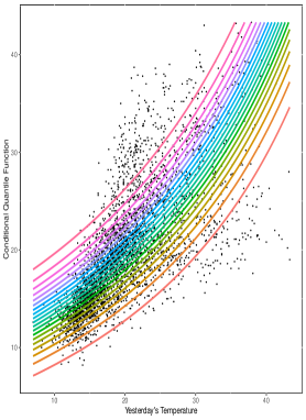
(a) Spec. 1.

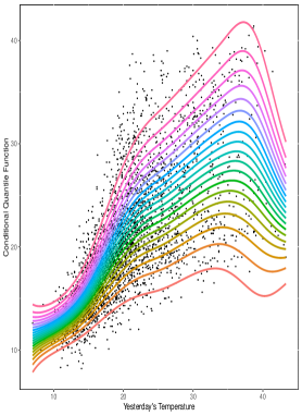
(b) Spec. 2.

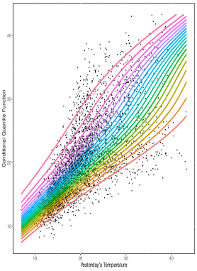
(c) Spec. 3.

Figure 6.1. CQF with scatterplot, for $u\in\{0.05,0.10,\ldots,0.95\}$.

Figure 6.1 shows CQFs for the models with smallest recorded BIC within each of the specification classes 1-3, illustrating the different features of the data that each specification class captures, as well as the corresponding restrictions on the implied distribution of $Y_{t}$ given $Y_{t-1}$. For both classes 1 and 2, this implied distribution is restricted to Gaussianity across all values of $Y_{t-1}$. Figure 6.1(A) shows that specification class 1 also strongly restricts the shape of the CQFs across values of $Y_{t-1}$, but is able to capture some nonlinearity in $Y_{t-1}$. Figure 6.1(B) shows that specification class 2 further allows for nonmonotonicity of the CQFs in $Y_{t-1}$, while capturing substantial heteroskedasticity in the data, a reflection of the more flexible functional forms for the conditional first and second moments of $Y_{t}$ given $Y_{t-1}$. In contrast with specification classes 1-2, for class 3 the GT $g^{*}(Y_{t},Y_{t-1})$ is nonlinear in $Y_{t}$ which allows for deviations of the conditional distribution of $Y_{t}$ given $Y_{t-1}$ from Gaussianity, through the dependence of the derivative function on both $Y_{t}$ and $Y_{t-1}$. Figure 6.1(C) illustrates the ability of specification class 3 to capture asymmetry of the distribution of $Y_{t}$ given $Y_{t-1}$, as well as changes in the mode location of this distribution across values of $Y_{t-1}$, in addition to allowing for nonlinearity of the CQF and heteroskedasticity.

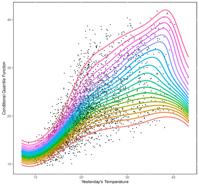
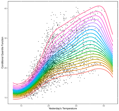
(a) CQF with scatterplot, for $u\in\{0.05,0.10,\ldots,0.95\}$.

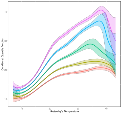
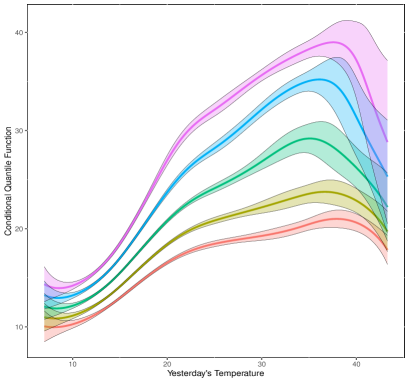
(b) CQF with confidence bands, for $u\in\{0.10,0.25,0.50,.0.75,0.90\}$.

Figure 6.2. Unpenalized (left) and penalized (right) CQF.

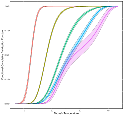
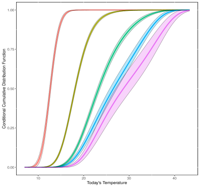
(a) Conditional CDF.

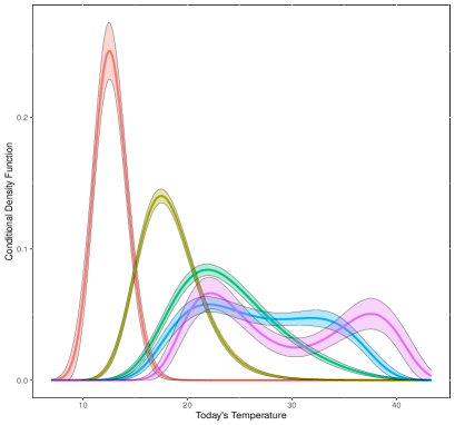
(b) Conditional PDF.

Figure 6.3. Unpenalized (left) and penalized (right) conditional PDF and CDF with confidence bands, for $y_{t-1}\in\{11.4,17.6,23.8,29.9,36.1\}$.

Figures 6.2-6.3 show distributional regression functions for the model specification with smallest BIC within the Spline-Spline specification class 4. The selected model has smallest BIC among all specification classes 1-4, and features quadratic splines in $s(Y_{t})$ with $J=5$, and cubic splines in $W(Y_{t-1})$ with $K=7$. In total, this parametrization includes 35 parameters, of which 25 are estimated to be nonzero after penalization. This parsimonious Spline-Spline model is able to simultaneously capture all important data features described above, including nonlinearity in $Y_{t-1}$ and the varying shape of the conditional distribution of $Y_{t}$. In particular, for the unpenalized CQF in Figure 6.2, the uneven spacing of the quantiles at higher values of lagged temperature suggests that the conditional PDF of current temperature is bimodal at such values. The two modes are especially apparent from the unpenalized PDFs displayed in 6.3(B), and are also reflected by the two inflection points in the corresponding CDF in Figure 6.3(A). The right panels of Figures 6.2-6.3 show the penalized versions of the distributional regression functions. In this example, the penalized estimator yields very similar conclusions, the main differences being the somewhat less pronounced bimodality for days with high temperatures, as well as the tighter confidence bands at the CQF boundaries.

Overall, we find that parsimonious Gaussian representations are able to capture complex features of the data, such as nonmonotonicity and conditional distributions with varying shapes, while providing complete estimates of distributional regression functions and their confidence bands. Importantly, the corresponding CQF estimates are endowed with the no-crossing property of quantiles over the full data support. In the Supplementary Material we assess the robustness of the selected Spline-Spline model and find that its main features are well-preserved across specifications with similar BIC values. Thus, although establishing the BIC properties in our context is an important topic for future research, we find that GT regression estimates of distributional regression functions exhibit reassuring stability within a given specification class.

7. Conclusion

The formulation of distributional regression models through the specification of a GT $e=g(Y,X)$ leads to a unifying framework for the global estimation of statistical objects of general interest, such as conditional quantile, density and distribution functions. The implied convex programming formulation is easy to implement and allows for estimation of sparse models. The linear form of the proposed GT regression models also constitutes a good starting point for nonparametric estimation of distributional regression functions. In this paper we have considered a few extensions to our original formulation such as misspecification, multiple outcomes and penalized estimation. Our framework can also be extended to allow for outcomes with discrete or mixed discrete-continuous distributions by appropriately modifying the form of the log-likelihood function. An important further extension we will consider in future work is the generalization of our results to distributional regression models with endogenous regressors.

Appendix A Proof of Theorem 1

For the conditional CDF of $Y$ given $X$, for all $y\in\mathbb{R}$,

(A.1) $$\Phi(b_{0}^{\prime}T(X,y))=\Pr[b_{0}^{\prime}T(X,Y)\leq b_{0}^{\prime}T(X,y)|X]=\Pr[Y\leq y|X]=F_{Y|X}(y|X),$$

where the first equality follows from $e=b_{0}^{\prime}T(X,Y)$ and $e|X\sim N(0,1)$, the second equality holds by $y\mapsto b_{0}^{\prime}T(X,y)$ strictly increasing with probability one by Lemma 1 below, and the last equality is by definition of $F_{Y|X}(y|X)$. For the conditional PDF, upon differentiating $y\mapsto\Phi(b_{0}^{\prime}T(X,y))$ and $y\mapsto F_{Y|X}(y|X)$ in (A.1), we obtain

$$\phi(b_{0}^{\prime}T(X,y))\{b_{0}^{\prime}t(X,y)\}=f_{Y\mid X}(y\mid X),\quad y\in\mathbb{R},$$

with probability one. For the CQF, the result in (A.1) and strict monotonicity of both $y\mapsto b_{0}^{\prime}T(X,y)$ and $e\mapsto\Phi(e)$ together imply $\Phi(b_{0}^{\prime}T(X,Q_{Y|X}(u|X)))=u$. Therefore, recalling that $e\mapsto h(X,e)$ is the inverse of $y\mapsto b_{0}^{\prime}T(X,y)$, we obtain

$$Q_{Y\mid X}(u\mid X)=h(X,\Phi^{-1}(u)),\quad u\in(0,1),$$

with probability one.∎

Lemma 1.

For each $b\in\Theta$, the mapping $y\mapsto\Phi(b^{\prime}T(X,y))$ is strictly increasing in $y\in\mathbb{R}$ with probability one.

Proof.

We note that $\partial_{y}\Phi(b^{\prime}T(X,y))=\phi(b^{\prime}T(X,y))\{b^{\prime}t(X,y)\}$ for all $y\in\mathbb{R}$, with $y\mapsto\phi(b^{\prime}T(X,y))\{b^{\prime}t(X,y)\}$ continuous, with probability one. Hence, for any $\alpha,\beta\in\mathbb{R}$, $\alpha<\beta$, by the Fundamental Theorem of Calculus,

$$\Phi(b^{\prime}T(X,\beta))-\Phi(b^{\prime}T(X,\alpha))=\int_{\alpha}^{\beta}\phi(b^{\prime}T(X,y))\{b^{\prime}t(X,y)\}dy>0,\quad b\in\Theta,$$

with probability one, since $b^{\prime}t(X,Y)>0$ and $\phi(e)>0$, $e\in\mathbb{R}$, which implies that $y\mapsto b^{\prime}T(X,y)$ is strictly increasing on $\mathbb{R}$, with probability one. ∎

Appendix B Proofs of Theorems 2-3 and Corollary 1

B.1. Definitions and notation

Define

$$L(Y,X,b)\equiv-\frac{1}{2}[\log(2\pi)+(b^{\prime}T(X,Y))^{2}]+\log(b^{\prime}t(X,Y)),\quad b\in\Theta,$$

and

$$f(Y,X,b)\equiv\phi(b^{\prime}T(X,Y))\{b^{\prime}t(X,Y)\},\quad b\in\Theta,$$

and note that

$$Q(b)=E[L(Y,X,b)]=E[\log f(Y,X,b)],\quad b\in\Theta.$$

In Appendix B.2 we establish the main properties of $Q(b)$ used in Appendix B.3 and B.5 for the proofs of Theorems 2 and 3, respectively.

B.2. Auxiliary lemmas

Lemma 2.

If Assumption 1 holds then $E[|L(Y,X,b)|]<\infty$ and $Q(b)$ is continuous over $\Theta$.

Proof.

By the triangle inequality,

$$E[|L(Y,X,b)|]\leq\frac{1}{2}E[|(b^{\prime}T(X,Y))^{2})|]+E[|\log(b^{\prime}t(X,Y))|]+\frac{1}{2}\log(2\pi).$$

The first term $E[|(b^{\prime}T(X,Y))^{2}|/2]$ is finite by Cauchy-Schwartz inequality and by $E[||T(X,Y)||^{2}]<\infty$. For the second term, applying a mean-value expansion around $\bar{b}=(b_{0},0_{JK-1})$, $b_{0}>0$, gives for some intermediate values $\tilde{b}$,

$$|\log(b^{\prime}t(X,Y))| =|\log(b_{0})+(\tilde{b}^{\prime}t(X,Y))^{-1}[(b-\bar{b})^{\prime}t(X,Y)]|$$

$$\leq|\log(b_{0})|+|(\tilde{b}^{\prime}t(X,Y))^{-1}|\,||b-\bar{b}||\,||t(X,Y)||.$$

Thus $E[|\log(b^{\prime}t(X,Y))|]<\infty$, since we have that $\tilde{b}^{\prime}t(X,Y)>0$ with probability one and $E[||t(X,Y)||]<\infty$. Therefore $E[|L(Y,X,b)|]<\infty$. Continuity of $Q(b)$ then follows from continuity of $b\mapsto L(Y,X,b)$ and dominated convergence. ∎

Lemma 3.

If Assumption 1 holds then $Q(b)$ is twice continuously differentiable over any compact subset $\overline{\Theta}\subset\Theta$, and $\nabla_{bb}E[L(Y,X,b)]=E[\nabla_{bb}L(Y,X,b)]$.

Proof.

By lemma 2, $E[|L(Y,X,b)|]<\infty$. Moreover, for $b\in\overline{\Theta}$,

$$||\nabla_{b}L(Y,X,b)|| =||-T(X,Y)(b^{\prime}T(X,Y))+(b^{\prime}t(X,Y))^{-1}t(X,Y)||$$

$$\leq||T(X,Y)(b^{\prime}T(X,Y))||+|(b^{\prime}t(X,Y))^{-1}|\,||t(X,Y)||$$

(B.1) $$\leq C\left\{||T(X,Y)||^{2}+||t(X,Y)||\right\},$$

for some finite constant $C>0$. Therefore, $E[||T(X,Y)||^{2}]<\infty$ and $E[||t(X,Y)||]<\infty$ imply that $E[\sup_{b\in\overline{\Theta}}||\nabla_{b}L(Y,X,b)||]<\infty$ under Assumption 1. Lemma 3.6 in Newey and McFadden (1994) then implies that $Q(b)$ is continuously differentiable in $b$, and that the order of differentiation and integration can be interchanged.

Continuous differentiability of $\nabla_{b}Q(b)$ in $b\in\overline{\Theta}$ follows from applying steps similar to (B.1). By

$$||\nabla_{bb}L(Y,X,b)||\leq||T(X,Y)||^{2}+C||t(X,Y)||^{2},$$

for some finite constant $C>0$, we have that $E[||T(X,Y)||^{2}]<\infty$ and $E[||t(X,Y)||^{2}]<\infty$ imply that $E[\sup_{b\in\overline{\Theta}}||\nabla_{bb}L(Y,X,b)||]<\infty$ under Assumption 1. Lemma 3.6 in Newey and McFadden (1994) then implies that $\nabla_{bb}Q(b)$ is continuously differentiable in $b$, and that the order of differentiation and integration can be interchanged. ∎

Lemma 4.

If Assumption 1 holds then, for any compact subset $\overline{\Theta}\subset\Theta$, we have that $-\nabla_{bb}Q(b)$ exists for $b\in\overline{\Theta}$, with smallest eigenvalue bounded away from zero uniformly in $b\in\overline{\Theta}$.

Proof.

By Lemma 3, $Q(b)$ is twice continuously differentiable over $\overline{\Theta}$ and the order of differentiation and integration can be interchanged. Therefore,

$$\nabla_{bb}\{-Q(b)\}=\Gamma_{1}+\Gamma_{2}(b),\;\Gamma_{1}\equiv E\left[T(X,Y)T(X,Y)^{\prime}\right],\;\Gamma_{2}(b)\equiv E\left[\frac{t(X,Y)t(X,Y)^{\prime}}{(b^{\prime}t(X,Y))^{2}}\right],$$

exists for all $b\in\overline{\Theta}$ under Assumption 1. Denoting the smallest eigenvalue of a matrix $A$ by $\lambda_{\min}(A)$, the result then follows from Weyl’s Monotonicity Theorem (e.g., Corollary 4.3.12 in Horn and Johnson, 2012) which implies

$$\lambda_{\min}(\Gamma_{1}+\Gamma_{2}(b))\geq\lambda_{\min}(\Gamma_{1})\geq B,\quad b\in\overline{\Theta},$$

for some constant $B>0$, by $\Gamma_{2}(b)$ being positive semidefinite for all $b\in\overline{\Theta}$ and the smallest eigenvalue of $E\left[T(X,Y)T(X,Y)^{\prime}\right]$ being bounded away from zero. ∎

B.3. Proof of Theorem 2

B.3.1. Uniqueness

We show that $b_{0}$ is a point of maximum of $Q(b)$ in $\Theta$. For $b\neq b_{0}$, $b\in\Theta$, by $E[\log f(Y,X,b_{0})]=E[\log f_{Y\mid X}(Y|X)]$ and Jensen’s inequality, we obtain

$$E\left[\log\left(\frac{f(Y,X,b_{0})}{f(Y,X,b)}\right)\right] =E\left[-\log\left(\frac{f(Y,X,b)}{f_{Y|X}(Y\mid X)}\right)\right]$$

$$\geq-\log E\left[\left(\frac{f(Y,X,b)}{f_{Y|X}(Y\mid X)}\right)\right]=-\log E\left[\int_{\mathbb{R}}f(y,X,b)dy\right]\geq 0,$$

since

$$\int_{\mathbb{R}}f(y,X,b)dy=\lim_{y\rightarrow\infty}\Phi(b^{\prime}T(X,y))-\lim_{y\rightarrow-\infty}\Phi(b^{\prime}T(X,y))\in(0,1]$$

with probability one, by the properties of the Gaussian CDF and $y\mapsto\Phi(b^{\prime}T(X,y))$ being strictly increasing by Lemma 1. Therefore, $b_{0}$ is a point of maximum. Strict concavity in Lemma 4 then implies that $Q(b)$ admits at most one maximizer in every compact subset in $\Theta$, and in particular every compact subset that contains $b_{0}$. Hence there is no $\widetilde{b}\neq b_{0}$ that maximizes $Q(b)$ in $\Theta$, and $b_{0}$ uniquely maximizes $Q(b)$ in $\Theta$.∎

B.3.2. Identification

By uniqueness of the point of maximum, for $b\neq b_{0}$, $b\in\Theta$, we have $E[\log f(Y,X,b_{0})]-E[\log f(Y,X,b)]>0$, which implies that $f(Y,X,b)\neq f(Y,X,b_{0})=f_{Y|X}(Y|X)$, and hence that $b_{0}$ is identified. Identification of $g(Y,X)$ and the distributional regression functions then follows by the fact that they are known functions of $b_{0}$, by Theorem 1.∎

B.4. Proof of Corollary 1

The proof follows by application of Theorem 2 and by the argument in the main text, using that $e=b_{0}^{\prime}T(Y,X)|X\sim N(0,1)$.

B.5. Proof of Theorem 3

B.5.1. Proof of existence of $b^{*}$

We first show that the level sets $\mathcal{B}_{\alpha}=\{b\in\Theta:-Q(b)\leq\alpha\}$, $\alpha\in\mathbb{R}$, of $-Q(b)$ are closed and bounded, hence compact, and then use the fact that $-Q(b)$ is continuous over $\Theta$, which implies existence of a minimizer.

Step 1. This step shows that $\mathcal{B}_{\alpha}$ is bounded.

Given $b_{1},b_{2}\in\mathcal{B}_{\alpha}$, let $t=||b_{1}-b_{2}||$ and $u=\frac{b_{1}-b_{2}}{||b_{1}-b_{2}||}$, so that $||u||=1$ and $b_{1}=b_{2}+tu$. By Lemma 3, $Q(b)$ is twice continuously differentiable for $b\in\mathcal{B}_{\alpha}$. Thus, by definition of $b_{1}$, a second-order Taylor expansion of $t\mapsto-Q(b_{2}+tu)$ around $t=0$ yields, for some $\bar{b}$ on the line connecting $b_{1}$ and $b_{2}$ and some constant $B>0$,

$$\alpha\geq-Q(b_{1})=-Q(b_{2}+tu) =-Q(b_{2})-t\nabla_{b}Q(b_{2})^{\prime}u-\frac{t^{2}}{2}u^{\prime}\nabla_{bb}Q(\bar{b})u$$

$$\geq-Q(b_{2})-t\nabla_{b}Q(b_{2})^{\prime}u+B\frac{t^{2}}{2}$$

$$\geq-Q(b_{2})-t||\nabla_{b}Q(b_{2})||+B\frac{t^{2}}{2},$$

where the penultimate inequality follows by Lemma 4. Fixing $b_{2}\in\mathcal{B}_{\alpha}$, the above inequality implies that $t$ is bounded and therefore $\mathcal{B}_{\alpha}$ is bounded.

Step 2. This step shows that $\mathcal{B}_{\alpha}$ is closed.

Define the boundary $\partial\Theta$ of $\Theta$ as

$$\partial\Theta=\{b\in\mathbb{R}^{JK}:\Pr[b^{\prime}t(X,Y)=0]>0\}.$$

For $b\in\partial\Theta$ with $b^{\prime}t(X,Y)<0$ on a set with positive probability, we adopt the convention that the logarithmic barrier function $\log(b^{\prime}t(X,Y))$ takes on the value $-\infty$ on that set (e.g., Section 11.2.1 in Boyd and Vandenberghe, 2004). Consider a sequence $(b_{n})$ in $\mathcal{B}_{\alpha}$ such that $b_{n}\rightarrow\check{b}\in\partial\Theta$ as $n\rightarrow\infty$. Steps 2.1 and 2.2 below show that $-Q(b_{n})=E[-L(Y,X,b_{n})]\rightarrow\infty$ as $n\rightarrow\infty$, and hence that $\mathcal{B}_{\alpha}$ is closed.

Step 2.1. This step shows that $E[\lim_{n\rightarrow\infty}-L(Y,X,b_{n})]\leq\lim_{n\rightarrow\infty}E[-L(Y,X,b_{n})]$.

By $\mathcal{B}_{\alpha}$ being bounded, there exists a constant $C>0$ such that $\log(b^{\prime}t(X,Y))\leq C||t(Y,X)||$ with probability one for all $b\in\mathcal{B}_{\alpha}$, and hence such that

$$-L(Y,X,b)=\frac{1}{2}[\log(2\pi)+(b^{\prime}T(X,Y))^{2}]-\log(b^{\prime}t(X,Y))\geq-C||t(X,Y)||,\quad b\in\mathcal{B}_{\alpha},$$

with probability one. Therefore,

$$\varphi(Y,X,b)\equiv-L(Y,X,b)+\delta(Y,X)\geq 0,\quad\delta(Y,X)\equiv C||t(X,Y)||,\quad b\in\mathcal{B}_{\alpha},$$

with probability one, and where $E[|\delta(Y,X)|]<\infty$ under Assumption 1.

Moreover, by definition of $\partial\Theta$, we have that $\lim_{n\rightarrow\infty}\log(b_{n}^{\prime}t(X,Y))=-\infty$ on a subset $\widetilde{\mathcal{YX}}$ of the joint support of $(Y,X)$ with positive probability, and hence

(B.2) $$\lim_{n\rightarrow\infty}-L(Y,X,b_{n})=\frac{1}{2}[\log(2\pi)+\lim_{n\rightarrow\infty}\{b_{n}^{\prime}T(X,Y)\}^{2}]-\lim_{n\rightarrow\infty}\log(b_{n}^{\prime}t(X,Y))=\infty,$$

on $\widetilde{\mathcal{YX}}$, by $\{b^{\prime}T(X,Y)\}^{2}/2\geq 0$ for all $b\in\mathbb{R}^{JK}$.

Letting $\chi_{\widetilde{\mathcal{YX}}}(Y,X)\equiv 1\{(Y,X)\in\widetilde{\mathcal{YX}}\}$ and $\chi_{\widetilde{\mathcal{YX}}^{c}}(Y,X)\equiv 1\{(Y,X)\in\widetilde{\mathcal{YX}}^{c}\}$, with $\widetilde{\mathcal{YX}}^{c}$ denoting the complement of $\widetilde{\mathcal{YX}}$, we have

$$E[\lim_{n\rightarrow\infty}\varphi(Y,X,b_{n})] =E[\chi_{\widetilde{\mathcal{YX}}}(Y,X)\lim_{n\rightarrow\infty}\varphi(Y,X,b_{n})]+E[\chi_{\widetilde{\mathcal{YX}}^{c}}(Y,X)\lim_{n\rightarrow\infty}\varphi(Y,X,b_{n})]$$

$$=E[\chi_{\widetilde{\mathcal{YX}}}(Y,X)\lim_{n\rightarrow\infty}-L(Y,X,b_{n})]+E[\chi_{\widetilde{\mathcal{YX}}}(Y,X)\delta(Y,X)\}]$$

$$+E[\chi_{\widetilde{\mathcal{YX}}^{c}}(Y,X)\lim_{n\rightarrow\infty}-L(Y,X,b_{n})]+E[\chi_{\widetilde{\mathcal{YX}}^{c}}(Y,X)\delta(Y,X)]$$

(B.3) $$=E[\lim_{n\rightarrow\infty}-L(Y,X,b_{n})]+E\left[\delta(Y,X)\right],$$

where the second equality follows from $\lim_{n\rightarrow\infty}-L(Y,X,b_{n})$ and $\delta(Y,X)$ being nonnegative functions on $\widetilde{\mathcal{YX}}$ (e.g., Proposition 5.2.6(ii) in Rana, 2002), and $\delta(Y,X)$ and $\lim_{n\rightarrow\infty}-L(Y,X,b_{n})$ having finite expectation on $\widetilde{\mathcal{YX}}^{c}$, since $\lim_{n\rightarrow\infty}b_{n}^{\prime}t(X,Y)>0$ on $\widetilde{\mathcal{YX}}^{c}$ and $E[|-L(Y,X,b)|]<\infty$ for all $b\in\Theta$ by Lemma 2.

By $\varphi(Y,X,b_{n})$ being nonnegative, Fatou’s lemma implies that

(B.4) $$E[\lim_{n\rightarrow\infty}\varphi(Y,X,b_{n})]\leq\lim_{n\rightarrow\infty}E[\varphi(Y,X,b_{n})],$$

with

(B.5) $$\lim_{n\rightarrow\infty}E[\varphi(Y,X,b_{n})]=\lim_{n\rightarrow\infty}E[-L(Y,X,b_{n})]+E[\delta(Y,X)],$$

by $E[|\delta(Y,X)|]<\infty$ and $E[|-L(Y,X,b_{n})|]<\infty$ for $b_{n}\in\Theta$ by Lemma 2. Therefore,

(B.6) $$E[\lim_{n\rightarrow\infty}-L(Y,X,b_{n})]\leq\lim_{n\rightarrow\infty}E[-L(Y,X,b_{n})]$$

follows by (B.3), (B.4) and (B.5) .

Step 2.2. This step shows that $E[\lim_{n\rightarrow\infty}-L(Y,X,b_{n})]=\infty$, and hence $\mathcal{B}_{\alpha}$ is closed.

The limit in (B.2) and the fact that $f_{YX}(Y,X)$ bounded away from 0 with probability one together imply that $E[\chi_{\widetilde{\mathcal{YX}}}(Y,X)\lim_{n\rightarrow\infty}-L(Y,X,b_{n})]=\infty$, and hence that $E[\chi_{\widetilde{\mathcal{YX}}}(Y,X)\lim_{n\rightarrow\infty}\varphi(Y,X,b_{n})]=\infty$ by $E[|\delta(Y,X)|]<\infty$. Moreover, $E[\chi_{\widetilde{\mathcal{YX}}^{c}}(Y,X)\lim_{n\rightarrow\infty}-L(Y,X,b_{n})]<\infty$, and hence $E[\chi_{\widetilde{\mathcal{YX}}^{c}}(Y,X)\lim_{n\rightarrow\infty}\varphi(Y,X,b_{n})]<\infty$ by $E[|\delta(Y,X)|]<\infty$. Therefore, $E[\lim_{n\rightarrow\infty}\varphi(Y,X,b_{n})]=\infty$, and (B.3) now implies that $E[\lim_{n\rightarrow\infty}-L(Y,X,b_{n})]=\infty$. This fact and the bound (B.6) together imply that $E[-L(Y,X,b_{n})]=-Q(b_{n})\rightarrow\infty$ as $n\rightarrow\infty$.

We have established that the limit $\check{b}$ of a convergent sequence $(b_{n})$ in $\mathcal{B}_{\alpha}$ is in $\Theta$. By continuity of $-Q(b)$ over $\Theta$, we then have that $-Q(\check{b})=\lim_{n\rightarrow\infty}Q(b_{n})\leq\alpha$, and hence $\check{b}\in\mathcal{B}_{\alpha}$ and $\mathcal{B}_{\alpha}$ is closed.

Step 3. This step concludes.

Pick $\alpha\in\mathbb{R}$ such that $\mathcal{B}_{\alpha}$ is nonempty. From Steps 1-2, $\mathcal{B}_{\alpha}$ is compact by the Heine-Borel theorem. Since $Q(b)$ is continuous over $\mathcal{B}_{\alpha}$, there is at least one minimizer to $-Q(b)$ in $\mathcal{B}_{\alpha}$ by the Weierstrass theorem. The existence result follows.∎

B.5.2. Proof of uniqueness of $b^{*}$

The uniqueness result follows by strict concavity of $Q(b)$ in Lemma 4∎

B.5.3. Proof of uniqueness of $g^{*}(Y,X)$, $F^{*}(Y,X)$, $Q^{*}(u,X)$ and $f^{*}(Y,X)$.

For $\widetilde{b}\neq b^{*}$, by nonsingularity of $E[T(X,Y)T(X,Y)^{\prime}]$ we have that

$$E[\{(\widetilde{b}-b^{*})^{\prime}T(X,Y)\}^{2}]=(\widetilde{b}-b^{*})^{\prime}E[T(X,Y)T(X,Y)^{\prime}](\widetilde{b}-b^{*})>0,$$

which implies $(\widetilde{b}-b^{*})^{\prime}T(X,Y)\neq 0$. Therefore, $g^{*}(Y,X)\neq\widetilde{m}(Y,X)$ for $\widetilde{m}\in\mathcal{E}$ with $\widetilde{b}\neq b^{*}$, by definition of $\mathcal{E}$. By strict monotonicity of $e\mapsto\Phi(e)$, this also implies that $\Phi(g^{*}(Y,X))\neq\Phi(\widetilde{m}(Y,X))$, and hence $F^{*}(Y,X)\neq\widetilde{F}(Y,X)$ for $\widetilde{F}\in\mathcal{F}$ with $\widetilde{m}\neq g^{*}$, by definition of $\mathcal{F}$. For $m\in\mathcal{E}$, let $\widetilde{\mathcal{Y}}_{x}(m)\equiv\{y\in\mathcal{Y}_{x}:F^{*}(y,x)\neq\Phi(m(y,x))\}$, where $\mathcal{Y}_{x}$ denotes the conditional support of $Y$ given $X=x$, and $\widetilde{\mathcal{U}}_{x}(m)\equiv\{u\in(0,1):F^{*}(y,x)=u\textrm{ for some }y\in\widetilde{\mathcal{Y}}_{x}(m)\}$. With probability one, by strict monotonicity of $y\mapsto m(y,X)$ for all $m\in\mathcal{E}$, the composition $y\mapsto\Phi(\widetilde{m}(y,X))$ is also strictly monotone, and hence $Q^{*}(\Phi^{-1}(u),X)\neq\widetilde{q}(X,\Phi^{-1}(u))$, $u\in\widetilde{\mathcal{U}}_{X}(\widetilde{m})$, for $\widetilde{q}\in\mathcal{Q}$ with $\widetilde{m}\neq g^{*}$, by definition of $\mathcal{Q}$. Finally, by $b^{*}$ being the unique maximizer of $Q(b)$ in $\Theta$, we have that $E[\log f^{*}(Y,X)]>E[\log(\phi(\widetilde{m}(Y,X))\{\partial_{y}\widetilde{m}(Y,X)\}]$ for $\widetilde{m}\in\mathcal{E}$ with $\widetilde{b}\neq b^{*}$, and hence $f^{*}(Y,X)\neq\widetilde{f}(Y,X)$ for $\widetilde{f}\in\mathcal{D}$ with $\widetilde{m}\neq g^{*}$, by definition of $\mathcal{D}$.∎

Appendix C Proof of Theorem 4

C.1. Auxiliary lemma

Lemma 5.

If the boundary conditions (3.2) hold for all $b\in\Theta$ with probability one, then the sets $\Theta$ and $\mathcal{D}$ are equivalent.

Proof.

Recall that two sets $\mathcal{A}$ and $\mathcal{B}$ are equivalent if there is a one-to-one correspondence between them, i.e., if there exists some function $\varphi:\mathcal{A}\rightarrow\mathcal{B}$ that is both one-to-one and onto. The two sets then have the same cardinality (Dudley, 2002).

We note that by nonsingularity of $E[T(X,Y)T(X,Y)^{\prime}]$ the two sets $\Theta$ and $\mathcal{E}$ are equivalent. Hence it suffices to show that $\mathcal{E}$ and $\mathcal{D}$ are equivalent. For each $f\in\mathcal{D}$, $m\in\mathcal{E}$, and $(y,x)\in\mathcal{YX}$, we define

$$(\varphi(f))(y,x)\equiv\Phi^{-1}\left(\int_{-\infty}^{y}f(t,x)dt\right),\quad(\psi(m))(y,x)\equiv\partial_{y}\Phi(m(y,x)),$$

We first verify that $\varphi:\mathcal{D}\rightarrow\mathcal{F}$ and $\psi:\mathcal{F}\rightarrow\mathcal{D}$, and then establish that $\varphi$ is one-to-one and onto by showing that $\varphi$ and $\psi$ are inverse functions of each other.

By definition of $f\in\mathcal{D}$, the Fundamental Theorem of Calculus, and the boundary conditions (3.2), we have

$$(\varphi(f))(y,X) =\Phi^{-1}\left(\int_{-\infty}^{y}\phi(T(X,v)^{\prime}b)\{b^{\prime}t(X,v)\}dv\right)$$

$$=\Phi^{-1}\left(\Phi(T(X,y)^{\prime}b)-\lim_{\alpha\rightarrow-\infty}\Phi(T(X,\alpha)^{\prime}b)\right)=T(X,y)^{\prime}b$$

for some $b\in\Theta$ and all $y\in\mathcal{Y}$, and hence $T(X,Y)^{\prime}b\in\mathcal{E}$. Therefore $\varphi:\mathcal{D}\rightarrow\mathcal{E}$. By definition of $m\in\mathcal{E}$ we have

$$(\psi(m))(y,X)=\partial_{y}\Phi(T(X,y)^{\prime}b)=\phi(T(X,y)^{\prime}b)\{t(X,y)^{\prime}b\},\quad y\in\mathcal{Y},$$

for some $b\in\Theta$, and hence $\phi(T(X,Y)^{\prime}b)\{t(X,Y)^{\prime}b\}\in\mathcal{D}$. Therefore $\varphi:\mathcal{E}\rightarrow\mathcal{D}$.

The conclusion then follows from $\psi$ being both the left-inverse of $\varphi$, since

$$(\psi(\varphi(f)))(y,X)=\partial_{y}\left\{\Phi\left(\Phi^{-1}\left(\int_{-\infty}^{y}f(t,X)dt\right)\right)\right\}=\partial_{y}\left\{\int_{-\infty}^{y}f(t,X)dt\right\}=f(y,X)$$

for all $y\in\mathcal{Y}$, and the right-inverse of $\varphi$, since

$$(\varphi(\psi(m)))(y,X)=\Phi^{-1}\left(\int_{-\infty}^{y}\partial_{y}\Phi(m(t,X))dt\right)=m(y,X),\quad y\in\mathcal{Y}.$$

Therefore, $\psi$ is the inverse function of $\varphi$ and the result follows. ∎

C.2. Proof of Theorem 4

By Theorem 3,

$$b^{*}=\arg\max_{b\in\Theta}E[\log(\phi(T(X,Y)^{\prime}b)\{t(X,Y)^{\prime}b\})].$$

Thus, $f(Y,X)=\phi(T(X,Y)^{\prime}b)\{t(X,Y)^{\prime}b\}\in\mathcal{D}$ for each $b\in\Theta$, and the fact that $\Theta$ and $\mathcal{D}$ are equivalent by Lemma 5, together imply that $f^{*}$ is the well-defined point of maximum of $E[\log f(Y,X)]$ in $\mathcal{D}$, and hence

$$f^{*} =\arg\max_{f\in\mathcal{D}}E\left[\log f(Y,X)\right]$$

(C.1) $$=\arg\min_{f\in\mathcal{D}}-E\left[\log f(Y,X)\right]=\arg\min_{f\in\mathcal{D}}E\left[\log\left(\frac{f_{Y|X}(Y\mid X)}{f(Y,X)}\right)\right].$$

Moreover, by the boundary conditions (3.2), each $f\in\mathcal{D}$ satisfies

(C.2) $$\int_{\mathbb{R}}f(y,X)dy=\lim_{y\rightarrow\infty}\Phi(b^{\prime}T(X,y))-\lim_{y\rightarrow-\infty}\Phi(b^{\prime}T(X,y))=1$$

for some $b\in\Theta$ with probability one. Therefore, (C.1) implies that $f^{*}(Y,X)$ is the KLIC closest probability distribution to $f_{Y|X}(Y|X)$ in $\mathcal{D}$.

By $F^{*}(Y,X)=\Phi(g^{*}(Y,X))$ and $f^{*}(Y,X)=\phi(g^{*}(Y,X))\{\partial_{y}g^{*}(Y,X)\}$, we have

$$\partial_{y}F^{*}(Y,X)=\phi(g^{*}(Y,X))\{\partial_{y}g^{*}(Y,X)\}=f^{*}(Y,X).$$

Since $y\mapsto f^{*}(y,X)$ is continuous, we obtain $F^{*}(y,X)=\int_{-\infty}^{y}f^{*}(t,X)dt$ for all $y\in\mathbb{R}$ by the Fundamental Theorem of Calculus, with $\lim_{y\rightarrow-\infty}F^{*}(y,X)=0$ and $\lim_{y\rightarrow\infty}F^{*}(y,X)=1$ by definition of $F^{*}(y,X)$ and (C.2).

By $f^{*}\in\mathcal{D}$ we have that $f^{*}(Y,X)>0$, and by Lemma 1 that $y\mapsto F^{*}(y,X)$ is strictly increasing, with probability one. Hence, the inverse function of $y\mapsto F^{*}(y,X)$ is well-defined, denoted $u\mapsto Q^{*}(X,u)$, with

$$\frac{\partial Q^{*}(X,u)}{\partial u}=\frac{1}{f^{*}(Q^{*}(X,u),X)}>0,\quad u\in(0,1),$$

with probability one, by continuous differentiability of $y\mapsto F^{*}(y,X)$ and the Inverse Function Theorem.∎

Appendix D Asymptotic Theory

D.1. Proof of Theorem 5

Parts (i)-(ii)

We verify the conditions of Theorem 2.7 in Newey and McFadden (1994). By Theorem 3, $b^{*}\in\Theta$ is the unique minimizer of $Q(b)$, and their Condition (i) is verified. By $\Theta$ convex and open, existence of $b^{*}\in\Theta$ established in Theorem 3 and concavity of $Q_{n}(b)$ together imply that their Condition (ii) is satisfied. Finally, since the sample is i.i.d. by Assumption 3(i), pointwise convergence of $Q_{n}(b)$ to $Q(b)$ follows from $Q(b)$ bounded (established in the proof of Theorem 2) and application of Khinchine’s law of large numbers. Hence, all conditions of Newey and McFadden’s Theorem 2.7 are satisfied. Therefore, there exists $\hat{b}\in\Theta$ with probability approaching one, and $\hat{b}\rightarrow_{p}b^{*}$.∎

Part (ii)

The asymptotic normality result $n^{1/2}(\hat{b}-b^{*})\overset{}{\rightarrow}_{d}N(0,\Gamma^{-1}\Psi(\Gamma^{-1})^{\prime})$ follows from verifying the assumptions of Theorem 3.1 in Newey and McFadden (1994), for instance. Symmetry and nonsingularity of $\Gamma$ then implies that $V=\Gamma^{-1}\Psi\Gamma^{-1}$.

By Theorem 3, $b^{*}$ is in the interior of $\Theta$ so that their Condition (i) is satisfied. Condition (ii) holds by inspection. Condition (iii) holds by $E[\psi(Y,X,b^{*})]=0$, existence of $\Gamma$ and the Lindberg-Levy central limit theorem.

For their Condition (iv), we apply Lemma 2.4 in Newey and McFadden (1994) with $a(Y,X,b)\equiv\nabla_{bb}L(Y,X,b)$. Let $\overline{\Theta}$ denote a compact subset of $\Theta$ containing $b^{*}$ in its interior. By the proof of Lemma 3 we have that $E[\sup_{b\in\overline{\Theta}}||\nabla_{bb}L(Y,X,b)||]<\infty$. In addition, by Assumption 3(i) the data is i.i.d., and $\nabla_{bb}L(Y,X,b)$ is continuous at each $b\in\overline{\Theta}$ by inspection. The conditions of the Lemma 2.4 in Newey and McFadden (1994) are verified, and therefore their Condition (iv) in Theorem 3.1 also is. Finally, $\Gamma$ is nonsingular by Lemma 4 which verifies their Condition (v). The result follows.

In order to show that $\hat{\Gamma}^{-1}\hat{\Psi}\hat{\Gamma}^{-1}\rightarrow_{p}\Gamma^{-1}\Psi\Gamma^{-1}$, we verify the conditions given in the discussion of Theorem 4.4 in Newey and McFadden (1994, bottom of page 2158). First, by Theorem 5 we have $\widehat{b}\rightarrow_{p}b^{*}$. Second, with probability one, by inspection $\log f(Y,X,b)$ is twice continuously differentiable and $f(Y,X,b)>0$ for all $b\in\Theta$. Moreover, $\Gamma$ exists and is nonsingular by Lemma 4. Thus Conditions (ii) and (iv) of Theorem 3.3 in Newey and McFadden (1994) are verified. Third,

$$||\psi(Y,X,b)||^{2} =||-T(X,Y)(b^{\prime}T(X,Y))+(b^{\prime}t(X,Y))^{-1}t(X,Y)||^{2}$$

$$\leq 2||T(X,Y)(b^{\prime}T(X,Y))||^{2}+2|(b^{\prime}t(X,Y))^{-1}|^{2}\,||t(X,Y)||^{2}$$

$$\leq C\left\{||T(X,Y)||^{4}+||t(X,Y)||^{2}\right\},$$

so that $E[\sup_{\theta\in\overline{\Theta}}||\psi(Y,X,b)||^{2}]<\infty$, by Assumption 1 and 3(ii). Hence, for a neighborhood $\mathcal{N}$ of $b^{*}$, we have that $E[\sup_{b\in\mathcal{N}}||\psi(Y,X,b)||^{2}]<\infty$. Moreover, $b\mapsto\psi(Y,X,b)$ is continuous at $b^{*}$ with probability one. The result follows.∎

D.2. Proof of Theorem 6

The proof builds on the proof strategy in Zou (2006) and Lu, Goldberg, and Fine (2012). Define

$$D_{n}(u)\equiv Q_{n}(b^{*}+n^{-1/2}u)-Q_{n}(b^{*}),$$

where $u$ is defined by $b=b^{*}+n^{-1/2}u$. Also let $\widehat{u}_{n}=\arg\max_{u}D_{n}(u)$, so that $\widehat{u}_{n}=\sqrt{n}(\widehat{b}_{\textrm{AL}}-b^{*})$. By a mean-value expansion,

$$D_{n}(u) =n^{-\frac{1}{2}}\sum_{i=1}^{n}\psi(y_{i},x_{i},b^{*})^{\prime}u+(2n)^{-1}u^{\prime}\left\{\sum_{i=1}^{n}\nabla_{b}\psi(y_{i},x_{i},\overline{b})\right\}u$$

$$+n^{-\frac{1}{2}}\lambda_{n}\sum_{l=1}^{JK}\widehat{w}_{l}n^{\frac{1}{2}}(|b_{l}^{*}|-|b_{l}^{*}+n^{-\frac{1}{2}}u_{l}|)\equiv D_{n}^{(1)}(u)+D_{n}^{(2)}(u)+D_{n}^{(3)}(u),$$

for some intermediate values $\overline{b}$. Under Assumptions 1-3, $D_{n}^{(1)}(u)\rightarrow_{d}N(0,u^{\prime}\Psi u)$ and $D_{n}^{(2)}(u)\rightarrow_{p}u^{\prime}\Gamma u$ by the results in Theorem 5 and the Law of Large Numbers. For $D_{n}^{(3)}(u)$, Zou (2006, proof of Theorem 2) shows

$$n^{-\frac{1}{2}}\lambda_{n}\widehat{w}_{l}n^{\frac{1}{2}}(|b_{l}^{*}|-|b_{l}^{*}+n^{-\frac{1}{2}}u_{l}|)\rightarrow_{p}\left\{\begin{array}[]{ccc}0,&b_{l}^{*}\neq 0\\ 0,&b_{l}^{*}=0,&u_{l}=0\\ -\infty,&b_{l}^{*}=0,&u_{l}\neq 0\end{array}\right..$$

Therefore $D_{n}(u)\rightarrow_{p}D(u)$ for every $u$, where

$$D(u)=\left\{\begin{array}[]{ccc}\frac{1}{2}u_{\mathcal{A}}^{\prime}\Gamma_{\mathcal{A}}u_{\mathcal{A}}+u_{\mathcal{A}}^{\prime}W,&u_{l}=0,&l\notin\mathcal{A},\\ -\infty&\textrm{otherwise},\end{array}\right.$$

with $W\sim N(0,\Psi_{\mathcal{A}})$. Moreover, steps similar to those of Lu, Goldberg, and Fine (2012, proof of Theorem 2) show that $\widehat{u}_{n}\rightarrow_{p}\widehat{u}$, upon using that $\widehat{w}_{l}\rightarrow_{p}1/b_{l}^{*}$ when $b_{l}^{*}\neq 0$ and $n^{1/2}\widehat{b}_{l}=O_{p}(1)$ when $b_{l}^{*}=0$ by Theorem 5(ii), and the fact that the Hessian matrix $\Gamma$ is negative definite by Lemma 4. This yields part (ii), i.e., $n^{1/2}(\widehat{b}_{\mathcal{A}}-b_{\mathcal{A}}^{*})\rightarrow_{d}N(0,\Gamma_{\mathcal{A}}^{-1}\Psi_{\mathcal{A}}\Gamma_{\mathcal{A}}^{-1})$. Steps similar to Lu, Goldberg, and Fine (2012, proof of Theorem 2) also show that $\Pr[\widehat{b}_{\mathcal{A}^{c}}=0]\rightarrow 1$, upon substituting for $Q_{n}(b)$ for their objective function, which establishes part (i).∎

D.3. Proof of Theorem 7

By Theorems 5 and 6 we have $n^{1/2}(\widehat{b}^{\dagger}-b^{*})\rightarrow_{d}N(0,\Xi)$ with $\Xi=\Gamma^{\dagger-1}\Psi^{\dagger}\Gamma^{\dagger-1}$ positive definite by assumption. Moreover, for $(y,x)\in\mathcal{YX}$, $b\mapsto\Phi(b^{\prime}T(x,y))\equiv F(y,x,b)$ and $b\mapsto f(y,x,b)$ are continuously differentiable, with derivative functions $\nabla_{b}F(y,x,b)=\phi(b^{\prime}T(x,y))T(x,y)$ and

$$\nabla_{b}f(y,x,b) =-\{b^{\prime}T(x,y)\}\phi(b^{\prime}T(x,y))\{b^{\prime}t(x,y)\}T(x,y)+\phi(b^{\prime}T(x,y))t(x,y)$$

$$=\phi(b^{\prime}T(x,y))\left[-\{b^{\prime}T(x,y)\}\{b^{\prime}t(x,y)\}T(x,y)+t(x,y)\right],$$

respectively, by the properties of the normal PDF. For all $(y,x)\in\mathcal{YX}$ with $f(y,x,b)>0$, $b\in\Theta$, we have that $y\mapsto F(y,x,b)$ is invertible, and its inverse function $u\mapsto F^{-1}(u,x,b)$ is continuously differentiable with derivative $1/f(F^{-1}(u,x,b),x,b)$ for all $x\in\mathcal{X}$ and $u\in\mathcal{U}_{x}(m)$, $m(y,x,b)\equiv b^{\prime}T(x,y)$, by the Inverse Function Theorem. Hence, by $F^{-1}(\Phi(b^{\prime}T(x,y)),x,b)=y$, we have for $(y,x)\in\mathcal{YX}$,

$$\nabla_{b}F^{-1}(\Phi(b^{\prime}T(x,y)),x,b)=\frac{\phi(b^{\prime}T(x,y))}{f(F^{-1}(u_{0},x,b),x,b)}T(x,y)+\nabla_{b}F^{-1}(u_{0},x,b)=0,$$

with $u_{0}=\Phi(b^{\prime}T(x,y))$, and hence, for $x\in\mathcal{X}$ and $u\in\mathcal{U}_{x}(m)$,

$$\nabla_{b}F^{-1}(u,x,b)=-\frac{\phi(b^{\prime}T(x,y_{0}))}{f(y_{0},x,b)}T(x,y_{0})=-\frac{1}{b^{\prime}t(x,y_{0})}T(x,y_{0})$$

where $y_{0}=F^{-1}(u,x,b)$, which is continuous in $b$ on $\Theta$, so that $b\mapsto F^{-1}(u,x,b)$ is continuously differentiable on $\Theta$. Parts (i) and (ii) in the statement of Theorem 7 then follow by application of the Delta method (e.g., Lemma 3.9 in Wooldridge, 2010).∎

Appendix E Duality Theory

E.1. Auxiliary lemma

In this Section, we write $T_{i}\equiv T(y_{i},x_{i})$ and $t_{i}\equiv t(y_{i},x_{i})$, for $i\in\{1,\ldots,n\}$. We first show the following result used in the proof of Theorem 8.

Lemma 6.

If $\{(y_{i},x_{i})\}_{i=1}^{n}$ is i.i.d. and $E[T(X,Y)T(X,Y)^{\prime}]$ is nonsingular then $\sum_{i=1}^{n}T_{i}T_{i}^{\prime}$ is nonsingular with probability approaching one.

Proof.

We note that $\sum_{i=1}^{n}T_{i}^{\prime}T_{i}$ is nonsingular if for all $\lambda\neq 0$ we have $\lambda^{\prime}(\sum_{i=1}^{n}T_{i}T_{i}^{\prime})\lambda=\sum_{i=1}^{n}(\lambda^{\prime}T_{i})^{2}>0$, and hence if, for some $i\in\{1,\ldots,n\}$, we have $\lambda^{\prime}T_{i}\neq 0$ for all $\lambda\neq 0$. By nonsingularity of $E[T(X,Y)T(X,Y)^{\prime}]$, for all $\lambda\neq 0$ we have $\lambda^{\prime}T(X,Y)\neq 0$ on a set $\widetilde{\mathcal{YX}}$ with $\Pr[\widetilde{\mathcal{YX}}]>0$. Hence for $\{(y_{i},x_{i})\}_{i=1}^{n}$ i.i.d.,

$$\Pr[\cap_{i\in\{1,\ldots,n\}}\{(y_{i},x_{i})\notin\widetilde{\mathcal{YX}}\}] =\prod_{i=1}^{n}\Pr[(y_{i},x_{i})\notin\widetilde{\mathcal{YX}}]$$

$$=\prod_{i=1}^{n}(1-\Pr[\widetilde{\mathcal{YX}}])=(1-\Pr[\widetilde{\mathcal{YX}}])^{n}\rightarrow 0,$$

as $n\rightarrow\infty$. Since the complement of the event $\cap_{i\in\{1,\ldots,n\}}\{(y_{i},x_{i})\notin\widetilde{\mathcal{YX}}\}$ is the event $\{(y_{i},x_{i})\in\widetilde{\mathcal{YX}}\textrm{ for some }i\in\{1,\ldots,n\}\}$, we obtain

$$\Pr[(y_{i},x_{i})\in\widetilde{\mathcal{YX}}\textrm{ for some }i\in\{1,\ldots,n\}]=1-(1-\Pr[\widetilde{\mathcal{YX}}])^{n}\rightarrow 1,$$

as $n\rightarrow\infty$. The result now follows from the definition of $\widetilde{\mathcal{YX}}$. ∎

E.2. Proof of Theorem 8

Part (i)

Let $\mathbb{R}_{-}\equiv(-\infty,0)$, $\mathbb{R}_{+}\equiv(0,+\infty)$. Introducing the variables $e_{i}=b^{\prime}T_{i}$, $\eta_{i}=b^{\prime}t_{i}$, an equivalent formulation for the GT regression problem is

$$\max_{(b,e,\eta)\in\Theta\times\mathbb{R}^{n}\times\mathbb{R}_{+}^{n}} n\kappa-\sum_{i=1}^{n}\left\{\frac{e_{i}^{2}}{2}-\log(\eta_{i})\right\},\quad\kappa\equiv-\frac{1}{2}\log(2\pi),$$

subject to $$e_{i}=b^{\prime}T_{i},\quad\eta_{i}=b^{\prime}t_{i},\quad i\in\{1,\ldots,n\}.$$

For all $(u,v)\in\mathbb{R}^{n}\times\mathbb{R}_{-}^{n}$, define the Lagrange function for this problem as

$$\mathscr{L}(b,e,\eta,u,v)=n\kappa-\sum_{i=1}^{n}\left\{\frac{e_{i}^{2}}{2}-\log(\eta_{i})\right\}+\sum_{i=1}^{n}u_{i}\left\{e_{i}-b^{\prime}T_{i}\right\}+\sum_{i=1}^{n}v_{i}\left\{\eta_{i}-b^{\prime}t_{i}\right\},$$

and the Lagrange dual function (Boyd and Vandenberghe (2004), Chapter 5) as

$$g(u,v) \equiv\sup_{(b,e,\eta)\in\Theta\times\mathbb{R}^{n}\times\mathbb{R}_{+}^{n}}\mathscr{L}(b,e,\eta,u,v)$$

$$=\sup_{(e,\eta)\in\mathbb{R}^{n}\times\mathbb{R}_{+}^{n}}\sum_{i=1}^{n}\left\{u_{i}e_{i}+v_{i}\eta_{i}-\left[-n\kappa+\frac{e_{i}^{2}}{2}-\log(\eta_{i})\right]\right\}$$

$$+\sup_{b\in\Theta}\left\{-\sum_{i=1}^{n}u_{i}(b^{\prime}T_{i})-\sum_{i=1}^{n}v_{i}(b^{\prime}t_{i})\right\}\equiv\textrm{$I_{1}$}+\textrm{$I_{2}$}.$$

In order to derive $g(u,v)$ we first show that for all $(u,v)\in\mathbb{R}^{n}\times\mathbb{R}_{-}^{n}$ the maximum of the mapping $(b,e,\eta)\mapsto\mathscr{L}(b,e,\eta,u,v)$ is attained and is unique, and we then evaluate $(b,e,\eta)\mapsto\mathscr{L}(b,e,\eta,u,v)$ at this value.

The first term $\textrm{I}_{1}$ in the dual function $g(u,v)$ is the convex conjugate of the negative log-likelihood function, defined as a function of the $n$-vectors $e$ and $\eta$. Define

$$\mathcal{D}(e,\eta,u,v)\equiv\sum_{i=1}^{n}\left\{u_{i}e_{i}+v_{i}\eta_{i}\right\}-\sum_{i=1}^{n}L(e_{i},\eta_{i}),\;L(e_{i},\eta_{i})\equiv-n\kappa+\frac{e_{i}^{2}}{2}-\log(\eta_{i}).$$

We first show that, for all $(u,v)\in\mathbb{R}^{n}\times\mathbb{R}_{-}^{n}$, the map $(e,\eta)\mapsto\mathcal{D}(e,\eta,u,v)$ admits at least one maximum in $\mathbb{R}^{n}\times\mathbb{R}_{+}^{n}$. For $i\in\{1,\ldots,n\}$, the first-order conditions are

$$\partial_{e_{i}}\mathcal{D}(e,\eta,u,v)=u_{i}-\sum_{i=1}^{n}\partial_{e_{i}}L(e_{i},\eta_{i}) =u_{i}-e_{i}=0$$

$$\partial_{\eta_{i}}\mathcal{D}(e,\eta,u,v)=v_{i}-\sum_{i=1}^{n}\partial_{\eta_{i}}L(e_{i},\eta_{i}) =v_{i}+\frac{1}{\eta_{i}}=0,$$

and upon solving for $e_{i}$ and $\eta_{i}$, we obtain

$$e_{i}=u_{i},\quad\eta_{i}=-\frac{1}{v_{i}},\quad i\in\{1,\ldots,n\}.$$

Clearly, for all $(u,v)\in\mathbb{R}^{n}\times\mathbb{R}_{-}^{n}$ there exists $(e,\eta)\in\mathbb{R}^{n}\times\mathbb{R}_{+}^{n}$ such that the $n$ first-order conditions hold.

We now show that, for all $(u,v)\in\mathbb{R}^{n}\times\mathbb{R}_{-}^{n}$, the map $(e,\eta)\mapsto\mathcal{D}(e,\eta,u,v)$ admits at most one maximum in $\mathbb{R}^{n}\times\mathbb{R}_{+}^{n}$. For $i\in\{1,\ldots,n\}$, the second-order conditions are

$$\partial_{e_{i},e_{i}}^{2}\mathcal{D}(e,\eta,u,v)=-1, \qquad\partial_{e_{i},\eta_{i}}^{2}\mathcal{D}(e,\eta,u,v)=0$$

$$\partial_{\eta_{i},e_{i}}^{2}\mathcal{D}(e,\eta,u,v)=0, \qquad\partial_{\eta_{i},\eta_{i}}^{2}\mathcal{D}(e,\eta,u,v)=-\frac{1}{\eta_{i}^{2}}.$$

Therefore the Hessian matrix of $(e,\eta)\mapsto\mathcal{D}(e,\eta,u,v)$ is negative definite for all $(u,v)\in\mathbb{R}^{n}\times\mathbb{R}_{-}^{n}$. Hence, $(e,\eta)\mapsto\mathcal{D}(e,\eta,u,v)$ is strictly concave with unique maximum $(e_{i},\eta_{i})=(u_{i},-1/v_{i})$, $i\in\{1,\ldots,n\}$, for all $(u,v)\in\mathbb{R}^{n}\times\mathbb{R}_{-}^{n}$. Evaluating $(e,\eta)\mapsto\mathcal{D}(e,\eta,u,v)$ at the maximum yields, for all $(u,v)\in\mathbb{R}^{n}\times\mathbb{R}_{-}^{n}$,

(E.1) $$\sup_{(e,\eta)\in\mathbb{R}^{n}\times\mathbb{R}_{+}^{n}}\mathcal{D}(e,\eta,u,v) = \sum_{i=1}^{n}u_{i}^{2}+\sum_{i=1}^{n}v_{i}\left(-\frac{1}{v_{i}}\right)-\sum_{i=1}^{n}\left\{-\kappa+\frac{u_{i}^{2}}{2}-\log\left(-\frac{1}{v_{i}}\right)\right\}$$

$$= -n(1-\kappa)+\sum_{i=1}^{n}\left\{\frac{u_{i}^{2}}{2}-\log\left(-v_{i}\right)\right\},$$

the conjugate function of the negative log-likelihood.

We now consider the second term $\textrm{I}_{2}$ in the definition of the dual function $g(u,v)$. For all $(b,u,v)\in\Theta\times\mathbb{R}^{n}\times\mathbb{R}_{-}^{n}$, define the penalty function

$$\mathcal{P}(b,u,v)=\sum_{i=1}^{n}\left\{-u_{i}(b^{\prime}T_{i})-v_{i}(b^{\prime}t_{i})\right\}.$$

The map $b\mapsto\mathcal{P}(b,u,v)$ is linear with partial derivative $-\sum_{i=1}^{n}\left\{u_{i}T_{i}+v_{i}t_{i}\right\}$. The value of $\sup_{b\in\Theta}\mathcal{P}(b,u,v)$ is thus determined by the set of all $(u,v)\in\mathbb{R}^{n}\times\mathbb{R}_{-}^{n}$ such that the first-order conditions,

(E.2) $$\nabla_{b}\mathcal{P}(b,u,v)=-\sum_{i=1}^{n}\left\{u_{i}T_{i}+v_{i}t_{i}\right\}=0,$$

hold. For all such $(u,v)\in\mathbb{R}^{n}\times\mathbb{R}_{-}^{n}$ and any solution $\overline{b}\in\Theta$, we have that

$$\sup_{b\in\Theta}\mathcal{P}(b,u,v)=\sum_{i=1}^{n}\left\{-u_{i}(\overline{b}^{\prime}T_{i})-v_{i}(\overline{b}^{\prime}t_{i})\right\}=-\overline{b}^{\prime}\sum_{i=1}^{n}\left\{u_{i}T_{i}+v_{i}t_{i}\right\}=0.$$

Therefore, for all $(u,v)\in\mathbb{R}^{n}\times\mathbb{R}_{-}^{n}$ such that $\nabla_{b}\mathcal{P}(\overline{b},u,v)=0$, the optimal value of $\mathcal{P}(\overline{b},u,v)$ is $0$.

Combining the expression for the likelihood conjugate (E.1) and the first-order conditions (E.2) gives the Lagrange dual function $g(u,v)$ for all $(u,v)$ such that $\nabla_{b}\mathcal{P}(b,u,v)=0$. The form of the dual GT regression problem (5.2) follows.

Part (ii)

The Lagrangian for (5.2) is

$$\mathcal{L}(u,v,b)=-n(1-\kappa)+\sum_{i=1}^{n}\left\{\frac{u_{i}^{2}}{2}-\log(-v_{i})\right\}-b^{\prime}\sum_{i=1}^{n}\left\{T_{i}u_{i}+t_{i}v_{i}\right\},$$

with first-order conditions

$$\partial_{u_{i}}\mathcal{L}(u,v,b)=u_{i}-b^{\prime}T_{i}=0,\quad\partial_{v_{i}}\mathcal{L}(u,v,b)=-\frac{1}{v_{i}}-b^{\prime}t_{i}=0,\quad i\in\{1,\ldots,n\},$$

equivalently, upon solving for $u_{i}$ and $v_{i}$,

(E.3) $$u_{i} =b^{\prime}T_{i},\quad v_{i}=-\frac{1}{b^{\prime}t_{i}},\quad i\in\{1,\ldots,n\}.$$

Upon substituting in the constraints of (5.2) we obtain the method-of-moments representation of (5.2).

Part (iii)

Existence of a solution $\widehat{b}\in\Theta$ is shown in the proof of Theorem 5(i). The sample Hessian matrix is $-\Sigma_{i=1}^{n}\{T_{i}T_{i}^{\prime}+t_{i}t_{i}^{\prime}/(b^{\prime}t_{i})^{2}\}$ which is negative definite with probability approaching one by Lemma 6. Therefore there exists a unique solution $\widehat{b}$ to the GT regression problem (4.1), with probability approaching one.

Existence of a solution $(\widehat{u}^{\prime},\widehat{v}^{\prime})^{\prime}$ to program (5.2) follows from existence of a solution $\widehat{b}\in\Theta$ to the first-order conditions of the ML problem (4.1) and the method-of-moments representation of the dual problem (5.2), upon setting $\widehat{u}_{i}=\widehat{b}^{\prime}T_{i}$, $\widehat{v}_{i}=-1/(\widehat{b}^{\prime}t_{i})$, for $i\in\{1,\ldots,n\}$. We now show that, for all $b\in\Theta$, the map $(u,v)\mapsto\mathcal{L}(u,v,b)$ admits at most one maximum in $\mathbb{R}^{n}\times\mathbb{R}_{-}^{n}$. For all $(u,v)\in\mathbb{R}^{n}\times\mathbb{R}_{-}^{n}$ and $i\in\{1,\ldots,n\}$, the second-order conditions for the dual problem (5.2) are

$$\partial_{u_{i},u_{i}}^{2}\mathcal{L}(u,v,b)=1, \qquad\partial_{u_{i},v_{i}}^{2}\mathcal{L}(u,v,b)=0$$

$$\partial_{v_{i},u_{i}}^{2}\mathcal{L}(u,v,b)=0, \qquad\partial_{v_{i},v_{i}}^{2}\mathcal{L}(u,v,b)=\frac{1}{v_{i}^{2}}.$$

Therefore, the Hessian matrix of $(u,v)\mapsto\mathcal{L}(u,v,b)$ is positive definite for all $b\in\Theta$. Hence, the map $(u,v)\mapsto\mathcal{L}(u,v,b)$ is strictly convex with unique solution $(\widehat{u}^{\prime},\widehat{v}^{\prime})^{\prime}$.

Part (iv)

Upon using (E.3) and with $\widehat{e}_{i}=\widehat{b}^{\prime}T_{i}$ and $\widehat{\eta}_{i}=\widehat{b}^{\prime}t_{i}$, $i\in\{1,\ldots,n\}$, the value of program (5.2) is

$$\mathcal{L}(\widehat{u},\widehat{v},\widehat{b})=-n(1-\kappa)+\sum_{i=1}^{n}\left\{\frac{\widehat{e}_{i}^{2}}{2}+\log\left(\widehat{\eta}_{i}\right)\right\}-\sum_{i=1}^{n}\left\{\widehat{e}_{i}^{2}-1\right\}=n\kappa-\sum_{i=1}^{n}\left\{\frac{\widehat{e}_{i}^{2}}{2}-\log\left(\widehat{\eta}_{i}\right)\right\},$$

the value of the ML problem (4.1) at a solution.

E.3. Proof of Theorem 9

Let $\left\|b\right\|_{1,\widehat{w}}=\sum_{l=1}^{JK}\widehat{w}_{l}|b_{l}|$. Analogously to the proof of Theorem 8(i), an equivalent formulation for the adaptive Lasso GT regression problem is

$$\max_{(b,e,\eta)\in\Theta\times\mathbb{R}^{n}\times\mathbb{R}_{+}^{n}} n\kappa-\sum_{i=1}^{n}\left\{\frac{e_{i}^{2}}{2}-\log(\eta_{i})\right\}-\lambda_{n}\left\|b\right\|_{1,\widehat{w}}$$

subject to $$e_{i}=b^{\prime}T_{i},\quad\eta_{i}=b^{\prime}t_{i},\quad i\in\{1,\ldots,n\},$$

and, letting $(u,v)\in\mathbb{R}^{n}\times\mathbb{R}_{-}^{n}$ denote Lagrange multiplier vectors, the corresponding Lagrange dual function can be written as

$$g(u,v) =\sup_{(e,\eta)\in\mathbb{R}^{n}\times\mathbb{R}_{+}^{n}}\sum_{i=1}^{n}\left\{u_{i}e_{i}+v_{i}\eta_{i}-\left[-n\kappa+\frac{e_{i}^{2}}{2}-\log(\eta_{i})\right]\right\}$$

$$+\sup_{b\in\Theta}\left\{-\sum_{i=1}^{n}u_{i}(b^{\top}T_{i})-\sum_{i=1}^{n}v_{i}(b^{\top}t_{i})-\lambda_{n}\left\|b\right\|_{1,\widehat{w}}\right\},$$

where the first term is the convex conjugate of $\sum_{i=1}^{n}\{-n\kappa+e_{i}^{2}/2-\log(\eta_{i})\}$ derived in the proof of Theorem 8(i).

For the second term, define

$$F(b)=\sum_{i=1}^{n}u_{i}(b^{\prime}T_{i})+\sum_{i=1}^{n}v_{i}(b^{\prime}t_{i})+\lambda_{n}\left\|b\right\|_{1,\widehat{w}},\quad b\in\mathbb{R}^{JK},$$

which is convex in $b$ but not smooth. In order to compute the subgradients of $F(b)$, we first compute the subgradients of $\left\|b\right\|_{1,\widehat{w}}$. Recalling that the weights satisfy $\widehat{w}_{l}>0$ for $\widehat{b}_{l}\neq 0$ and $\widehat{w}_{l}=0$ otherwise, the weighted norm $\left\|b\right\|_{1,\widehat{w}}$ can be written as the maximum of $2^{n}$ linear functions:

$$\left\|b\right\|_{1,\widehat{w}}=\max\left\{s^{\prime}b:s_{l}\in\{-\widehat{w}_{l},\widehat{w}_{l}\}\right\}.$$

The functions $s^{\prime}b$ are differentiable and have a unique subgradient $s$. The subdifferential of $\left\|b\right\|_{1,\widehat{w}}$ is given by all convex combinations of gradients of the active functions at $b$ (Boyd and Vandenberghe, 2008). We first identify an active function $s^{\prime}b$, by finding an $s=(s_{1},\ldots,s_{JK})^{\prime}$, $s_{l}\in\{-\widehat{w}_{l},\widehat{w}_{l}\}$, such that $s^{\prime}b=\left\|b\right\|_{1,\widehat{w}}$. Choose $s_{l}=\widehat{w}_{l}$ if $b_{l}>0$, and $s_{l}=-\widehat{w}_{l}$ if $b_{l}<0$, for each $l$. If $b_{l}=0$, choose either $s_{l}=-\widehat{w}_{l}$ or $s_{l}=\widehat{w}_{l}$. We can therefore take

$$z_{l}=\begin{cases}\widehat{w}_{l}&\textrm{if }b_{l}>0\\ -\widehat{w}_{l}&\textrm{if }b_{l}<0\\ -\widehat{w}_{l}\textrm{ or }\widehat{w}_{l}&\textrm{if }b_{l}=0\end{cases},\quad l\in\{1,\ldots,JK\}.$$

The subdifferential of $\left\|b\right\|_{1,\widehat{w}}$ is:

$$\partial\left\|b\right\|_{1,\widehat{w}}=\left\{z:|z_{l}|\leq\widehat{w}_{l},\;l\in\{1,\ldots,JK\},\;z^{\prime}b=\left\|b\right\|_{1,\widehat{w}}\right\}.$$

Therefore, the subgradient of $F(b)$ is:

$$\partial F(b)=\left\{\sum_{i=1}^{n}u_{i}T_{i.l}+\sum_{i=1}^{n}v_{i}t_{i.l}+\lambda_{n}z_{l},\quad l\in\{1,\ldots,JK\}\right\},$$

where $|z_{l}|\leq\widehat{w}_{l}$, $l\in\{1,\ldots,JK\}$, and $z^{\prime}b=\left\|b\right\|_{1,\widehat{w}}$ , i.e., $z$ is the subgradient of $\left\|b\right\|_{1,\widehat{w}}$.

The subgradient optimality condition is that there exists $\overline{b}$ such that $0\in\partial F(\overline{b})$. Thus $\overline{b},\overline{z}$ should satisfy

$$\overline{z}_{l}=-\sum_{i=1}^{n}\left\{u_{i}T_{i,l}+v_{i}t_{i,l}\right\}/\lambda_{n},\quad|\overline{z}_{l}|\leq\widehat{w}_{l},\quad\overline{z}^{\prime}\overline{b}=||\overline{b}||_{1,\widehat{w}},\quad l\in\{1,\ldots,JK\},$$

which is equivalent to

(E.4) $$\left|\sum_{i=1}^{n}\left\{T_{i,l}u_{i}+t_{i,l}v_{i}\right\}\right|\leq\lambda_{n}\widehat{w}_{l},\quad l\in\{1,\ldots,JK\}.$$

Upon substituting into $F(b)$ gives

$$F(\overline{b}) =\inf_{b\in\Theta}F(b)=\sum_{i=1}^{n}u_{i}(\overline{b}^{\prime}T_{i})+\sum_{i=1}^{n}v_{i}(\overline{b}^{\prime}t_{i})+\lambda_{n}\sum_{l=1}^{JK}\frac{-\sum_{i=1}^{n}\left\{u_{i}T_{i,l}+v_{i}t_{i,l}\right\}}{\lambda_{n}}\overline{b}_{l}$$

$$=\sum_{i=1}^{n}\left\{u_{i}(\overline{b}^{\prime}T_{i})+v_{i}(\overline{b}^{\prime}t_{i})\right\}-\sum_{i=1}^{n}\left\{u_{i}\sum_{l=1}^{JK}T_{i,l}\overline{b}_{l}+v_{i}\sum_{l=1}^{JK}t_{i,l}\overline{b}_{l}\right\}=0.$$

Hence the optimal value of $F(b)$ is $0$, and combining the expression for the likelihood conjugate (E.1) and the optimality conditions (E.4) gives the Lagrange dual function $g(u,v)$ for all $(u,v)$ such that (E.4) holds. The form of (4.2) follows.

References

• Andrews (1997) Andrews, D. (1997). A conditional Kolmogorov test. Econometrica (65, September), pp. 1097–1128.
• Boyd and Vandenberghe (2004) Boyd, S. P. and Vandenberghe, L. (2004). Convex Optimization. Cambridge University Press.
• Boyd and Vandenberghe (2008) Boyd, S. P. and Vandenberghe, L. (2008). Subgradients. Notes for EE364b. Stanford University, Winter 2006, 7, pp.1-7.
• Chen, Goldstein, and Shao (2010) Chen, L.H., Goldstein, L. and Shao, Q.M. (2010). Normal approximation by Stein’s method. Springer Science & Business Media.
• Chernozhukov, Fernandez-Val, and Galichon (2010) Chernozhukov, V., Fernandez-Val, I., and Galichon, A. (2010). Quantile and probability curves without crossing. Econometrica 78(3, May), pp. 1093–1125.
• Chernozhukov, Fernandez-Val, and Melly (2013) Chernozhukov, V., Fernandez-Val, I., and Melly, B. (2013). Inference on counterfactual distributions. Econometrica 81(6, November), pp. 2205–2268.
• Chernozhukov, Wutrich, and Zhu (2019) Chernozhukov, V., Wüthrich, K., and Zhu, Y. (2019). Distributional conformal prediction. eprint arXiv:1909.07889.
• Chernozhukov, Fernandez-Val, Newey, Stouli, and Vella (2020) Chernozhukov, V., Fernandez-Val, I., Newey, W., Stouli, S., and Vella, F. (2020). Semiparametric estimation of structural functions in nonseparable triangular models. Quantitative Economics 11, pp. 503–533.
• Chesher (2003) Chesher, A. (2003). Identification in nonseparable models. Econometrica (71, September), pp. 1405–1441.
• Chesher and Spady (1991) Chesher, A. and Spady, R. H. (1991). Asymptotic expansions of the information matrix test statistic. Econometrica (59, May), pp. 787–815.
• Curry and Schoenberg (1966) Curry, H. B. and Schoenberg, I. J. (1966). On Polya frequency functions IV: The fundamental spline functions and their limits. J. Analyse Math. 17, pp.71–107, 1966.
• DiNardo, Fortin, and Lemieux (1996) DiNardo, J., Fortin, N.M. and Lemieux, T. (1996). Labor market institutions and the distribution of wages, 1973-1992: A semiparametric approach. Econometrica 64(5), pp.1001–1044.
• Domahidi, Chu, and Boyd (2013) Domahidi A., Chu, E., and Boyd, S. (2013). ECOS: an SOCP Solver for embedded systems. In Proceedings of the European Control Conference, pp. 3071–3076.
• Dudley (2002) Dudley, R.M. (2002). Real Analysis and Probability. Cambridge University Press, 2nd Edition.
• Foresi and Perrachi (1995) Foresi, S. and Peracchi, F. (1995). The conditional distribution of excess returns: An empirical analysis. Journal of the American Statistical Association, 90(430), pp. 451–466.
• Fu, Narasimhan, and Boyd (2017) Fu, A., Narasimhan, B. and Boyd, S. (2017). CVXR: An R package for disciplined convex optimization. arXiv preprint arXiv:1711.07582.
• Hall, Wolff, and Yao (1999) Hall, P., Wolff, R.C. and Yao, Q. (1999). Methods for estimating a conditional distribution function. Journal of the American Statistical Association, 94(445), pp.154–163.
• Horn and Johnson (2012) Horn, R. A. and Johnson, C. R. (2012). Matrix Analysis. 2nd ed., Cambridge University Press.
• Horowitz and Nesheim (2020) Horowitz, J. and Nesheim, L. (2020). Using penalized likelihood to select parameters in a random coefficients multinomial logit model. Journal of Econometrics, forthcoming.
• Hyndman, Bashtannyk, and Grunwald (1996) Hyndman, R.J., Bashtannyk, D.M. and Grunwald, G.K. (1996). Estimating and visualizing conditional densities. Journal of Computational and Graphical Statistics, 5(4), pp.315–336.
• Imbens and Newey (2009) Imbens, G. and Newey, W. K. (2009). Identification and estimation of triangular simultaneous equations models without additivity. Econometrica 77(5, September), pp. 1481–1512.
• Koenker (2000) Koenker, R. (2000). Galton, Edgeworth, Frisch, and prospects for quantile regression in econometrics. Journal of Econometrics 95(2), pp. 347–374.
• Koenker and Basset (1978) Koenker, R. and Bassett, G. (1978). Regression quantiles. Econometrica (46), pp. 33–50.
• Kooperberg and Stone (2001) Kooperberg, C. and Stone, C. J. (1991). A study of logspline density estimation. Computational Statistics & Data Analysis 12(3), pp. 327–347.
• Lu, Goldberg, and Fine (2012) Lu, W., Goldberg, Y., and Fine, J. P. (2012). On the robustness of the adaptive lasso to model misspecification. Biometrika 99, pp. 717–731.
• Matzkin (2003) Matzkin, R. (2003). Nonparametric estimation of nonadditive random functions. Econometrica (71, September), pp. 1339–1375.
• Newey and McFadden (1994) Newey, W. and Mc Fadden, D. (1994). Large sample estimation and hypothesis testing. In Handbook of Econometrics, vol. 4, ch. 36, 1st ed., pp. 2111–2245. Amsterdam: Elsevier.
• O’Donoghue, Chu, Parikh, and Boyd (2016) O’donoghue, B., Chu, E., Parikh, N. and Boyd, S. (2016). Conic optimization via operator splitting and homogeneous self-dual embedding. Journal of Optimization Theory and Applications , 169(3), pp. 1042–1068.
• Owen (2007) Owen, A. B. (2007). A robust hybrid of lasso and ridge regression. Contemporary Mathematics 443(7), pp. 59-72.
• R Development Core Team (2020) R Development Core Team (2020). R: A language and environment for statistical computing. Vienna, Austria: R Foundation for Statistical Computing.
• Ramsay (1988) Ramsay, J. O. (1988). Monotone regression splines in action. Statistical Science 3(4), pp.425-441.
• Rana (2002) Rana, I. K. (2002). An Introduction to Measure and Integration. Vol. 45. American Mathematical Soc..
• Rosenblatt (1952) Rosenblatt, M. (1952). Remarks on a multivariate transformation. The Annals of Mathematical Statistics 23(3), pp.470–472.
• Spady and Stouli (2018a) Spady, R. H. and Stouli, S. (2018a). Dual regression. Biometrika 105, pp. 1–18.
• Spady and Stouli (2018b) Spady, R. H. and Stouli, S. (2018b). Simultaneous mean-variance regression. eprint arXiv:1804.01631.
• White (1982) White, H. (1982). Maximum likelihood estimation of misspecified models. Econometrica (50, January), pp. 1–25.
• Wooldridge (2010) Wooldridge, J. M. (2010). Econometric analysis of cross section and panel data. MIT Press.
• Zou (2006) Zou, H. (2006). The adaptive lasso and its oracle properties. Journal of the American statistical association, 101(476), pp.1418–1429.