First steps toward a simple but efficient model-free control synthesis for variable-speed wind turbines

Abstract

Although variable-speed three-blade wind turbines are nowadays quite popular, their control remains a challenging task. We propose a new easily implementable model-free control approach with the corresponding intelligent controllers. Several convincing computer simulations, including some fault accommodations, shows that model-free controllers are more efficient and robust than classic proportional-integral controllers.

I Introduction

Wind energy has been the focus of growing interest for many years. Improving the performances and profitability of wind turbines is currently a burgeoning research topic. Deriving efficient control strategies plays therefore a key rôle (see, e.g., [1, 2, 3, 4, 5]). Advanced techniques are often investigated in the academic literature.

Our study concerns the three-blade machines. They gradually became dominant during the late 1980s. To control such a turbine, a distinction (Fig. 1) is made between the variable speed operating mode (low-speed region) and the power regulation mode (high-speed region) [6, 7]. In the low-speed region, the wind turbine operates under the nominal power. The purpose of the control is to make maximum use of wind energy and to vary the rotor speed according to the generator torque. In the high-speed region, blade pitch and generator torque can be used for power control. The objective is no longer to maximize the wind energy capture but rather to regulate the energy produced around a nominal value, i.e., around the rated electrical power $P_{\rm rated}$ of the turbine: See Fig. 1.

Although the severe shortcomings of Proportional-Integral (PI) and Proportional-Integral-Derivative (PID) controllers are well known [8, 9], they remain most popular in the industrial world, including wind turbines. Therefore they are still studied in the academic literature on wind turbines [10, 11, 12].

This paper is devoted to the utilization of model-free control (MFC) in the sense of [13]:

• It keeps the benefits of PIs and PIDs, and, especially, the futility of almost any mathematical modeling.

• Most of the deficiencies of PIs and PIDs are mitigated.

• Its implementation turns out to be often simpler, when compared to PIs and PIDs.

MFC has been successfully applied all over the world as demonstrated by the references in [13, 14, 15]. See already [16, 17] for its relevance to wind turbine. We show here the interest of MFC to control the pitch angle and the generator torque for low and high winds.

Remark 1

The enormous difficulty of writing down a suitable mathematical modeling of wind turbines explains why other model-free settings have been proposed (see, e.g., [18]). They are mostly based on various optimization techniques.

Remark 2

A patent (Électricité de France (EDF) and École polytechnique) has been associated to the use of MFC for hydroelectric power plants [19], i.e., to another green energy production.

Our paper is organized as follows. For the sake of computer simulations Section II provide short mathematical descriptions of wind turbines and of the wind. MFC is briefly recalled in Section III. Computer simulations are presented in Section IV where fault accommodations are considered: They show a striking superiority of MFC with respect to a classical PI. Some concluding suggestions for future research are sketched in Section V.

II Mathematical modelings for
computer simulations

II-A Wind turbine

Let us emphasize that the model below is more or less improper for deriving control laws. What follows is borrowed from [7, 20, 21, 22].

See Table I for some useful parameters where

TABLE I: Wind turbine parameters

Variable	Value
$J_{\rm t}$ ($kgm^{2}$)	$3.89\cdot 10^{5}$
$K_{\rm t}$ ($Nm/rad/s$)	400
$\rho$ ($kgm^{3}$)	1.29
R ($m$)	21.65
$max\ T_{g}$ ($kNm$)	162
$P_{\rm rated}$ ($kW$)	600

• $\rho$ is the air density (kg/m³),

• $R$ is the radius of the blade (m),

• $V$ is the wind speed (m/s),

• $T_{\text{g}}$ is the generator torque (Nm),

• ${\rm max}\ T_{\rm g}$ is the maximum value of $T_{\text{g}}$,

• $J_{\rm t}$ is the combined inertia of the turbine and generator (kgm²),

• $K_{\rm t}$ is the the damping coefficient of the turbine (Nm/rad/s),

• $C_{p}\left(\lambda,\beta\right)$ is the power conversion coefficient. It depends on the tip-speed ratio $\lambda$ and the pitch angle $\beta$:

  $$C_{p}\left(\lambda,\beta\right)=c_{1}\left(\frac{c_{2}}{\lambda_{i}}-c_{3}\beta-c_{4}\right)\exp\left(\frac{-c_{5}}{\lambda_{i}}\right)+c_{6}\lambda$$

  $$\frac{1}{\lambda_{i}}=\frac{1}{\lambda+0.08\beta}-\frac{0.035}{\beta^{3}+1}$$

  See Table II for the coefficients $c_{\kappa}$, $\kappa=1,\dots,6$.

  TABLE II: Coefficients for the power conversion coefficient

  Coefficient	Value
  $c_{\rm 1}$	0.4
  $c_{\rm 2}$	116
  $c_{\rm 3}$	0.4
  $c_{\rm 4}$	5
  $c_{\rm 5}$	21
  $c_{\rm 6}$	0.02

The output power of wind turbines is given by

$$P_{t}\ (W)=\frac{1}{2}\rho\pi R^{2}C_{p}\left(\lambda,\beta\right)V^{3}$$

The tip-speed ratio is defined by

$$\lambda=\frac{R\omega_{t}}{V}$$

where $\omega_{t}$ is the turbine angular speed (rad/s).

Write the turbine torque

$$T_{\rm t}=\frac{1}{2}\rho\pi R^{3}V^{2}\frac{C_{p}\left(\lambda,\beta\right)}{\lambda}$$

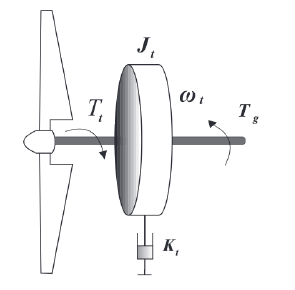
Figure 2: One-mass model of a wind turbine [22]

If a perfectly rigid low-speed shaft is assumed, a one-mass model of the turbine (see Fig. 2) may be expressed by

$$J_{\rm t}\dot{\omega}_{\rm t}=T_{\rm t}-K_{\rm t}\omega_{\rm t}-T_{\text{g}}$$

II-B Wind

The wind speed $V$ may vary considerably. Its variation may be modeled as a finite sum of harmonics in the frequency range 0.1-10 Hz:

$$V=V_{\text{moy}}\left[1+\sum_{\rm finite}A_{k}\sin(\omega_{k}t)\right]$$ (1)

$V_{\text{moy}}$ is the mean speed, $A_{k}$ is the magnitude of the $k$th sine wave of frequency $\omega_{k}$ [23]. Eq. (1) reads here

$$V=V_{\text{moy}}\left[1+A_{1}\sin(0.1047t)+A_{2}\sin(0.2674t)\right.\\ \left.+A_{3}\sin(1.309t)+A_{4}\sin(3.696t)\right]$$

See Table III for the coefficients $A_{\iota}$, $\iota=1,\dots,4$.

TABLE III: Coefficient magnitudes with respect to the mean wind speed

Mean wind speed	Coefficients
$V_{\text{moy}}$ (m/s)	$A_{1}$	$A_{2}$	$A_{3}$	$A_{4}$
7	0.029	0.286	0.143	0.029
8	0.025	0.25	0.125	0.025
9	0.022	0.222	0.111	0.022
16	0.0125	0.125	0.0625	0.0125
20	0.01	0.1	0.05	0.01

III Model-free control
and intelligent controllers

For the sake of notational simplicity, let us restrict ourselves to single-input single-output (SISO) systems.

III-A The ultra-local model

The unknown global description of the plant is replaced by the following first-order ultra-local model:

$$\boxed{\dot{y}=F+\alpha u}$$ (2)

where:

1. The control and output variables are respectively $u$ and $y$.

2. $\alpha\in\mathbb{R}$ is chosen by the practitioner such that the three terms in Equation (2) have the same magnitude.

The following comments are useful:

• $F$ is data driven: it is given by the past values of $u$ and $y$.

• $F$ includes not only the unknown structure of the system but also any disturbance.

III-B Intelligent controllers

Close the loop with the intelligent proportional controller, or iP,

$$\boxed{u=-\frac{F_{\text{est}}-\dot{y}^{\ast}+K_{P}e}{\alpha}}$$ (3)

where

• $y^{\ast}$ is the reference trajectory,

• $e=y-y^{\star}$ is the tracking error,

• $F_{\text{est}}$ is an estimated value of $F$

• $K_{P}\in\mathbb{R}$ is a gain.

Equations (2) and (3) yield

$$\dot{e}+K_{P}e=F-F_{\text{est}}$$

If the estimation $F_{\text{est}}$ is “good”: $F-F_{\text{est}}$ is “small”, i.e., $F-F_{\text{est}}\simeq 0$, then $\lim_{t\to+\infty}e(t)\simeq 0$ if $K_{P}>0$. It implies that the tuning of $K_{P}$ is straightforward. This is a major benefit when compared to the tuning of “classic” PIDs (see, e.g., [8, 9, 24]).

III-C Estimation of $F$

Mathematical analysis [25] tells us that under a very weak integrability assumption, any function, for instance $F$ in Eq. (2), is “well” approximated by a piecewise constant function.

III-C1 First approach

Rewrite then Eq. (2) in the operational domain [26]:

$$sY=\frac{\Phi}{s}+\alpha U+y(0)$$

where $\Phi$ is a constant. We get rid of the initial condition $y(0)$ by multiplying both sides on the left by $\frac{d}{ds}$:

$$Y+s\frac{dY}{ds}=-\frac{\Phi}{s^{2}}+\alpha\frac{dU}{ds}$$

Noise attenuation is achieved by multiplying both sides on the left by $s^{-2}$, i.e., via integration [27]. It yields in the time domain the real-time estimate, thanks to the equivalence between $\frac{d}{ds}$ and the multiplication by $-t$,

$${\small F_{\text{est}}(t)=-\frac{6}{\tau^{3}}\int_{t-\tau}^{t}\left[(\tau-2\sigma)y(\sigma)+\alpha\sigma(\tau-\sigma)u(\sigma)\right]d\sigma}$$

where $\tau>0$ might be quite small. This integral, which is a low pass filter, may of course be replaced in practice by a classic digital filter.

III-C2 Second approach

Close the loop with the iP (3). It yields:

$$F_{\text{est}}(t)=\frac{1}{\tau}\left[\int_{t-\tau}^{t}\left(\dot{y}^{\star}-\alpha u-K_{P}e\right)d\sigma\right]$$

Remark 3

Let us emphasize that implementing our intelligent controllers is easy [13], [28].

III-D MIMO systems

Consider a multi-input multi-output (MIMO) system with $m$ control variables $u_{i}$ and $m$ output variables $y_{i}$, $i=1,\dots,m$, $m\geq 2$. It has been observed in [29] and confirmed by all encountered concrete case-studies (see, e.g., [30]), that such a system may usually be regulated via $m$ monovariable ultra-local models:

$$y_{i}^{(n_{i})}=F_{i}+\alpha_{i}u_{i}$$

where $F_{i}$ may also depend on $u_{j}$, $y_{j}$, and their derivatives, $j\neq i$.

IV Simulation results

Write $P_{\rm e}$ the electrical power of the turbine. Define, according to Fig. 1, the following regions:

• Low-speed region: $V_{\rm cut-in}\leq V<V_{\rm rated}$, $P_{\text{e}}<P_{\rm rated}$.

• High-speed region: $V_{\rm rated}\leq V\leq V_{\rm cut-off}$, $P_{\text{e}}=P_{\rm rated}$.

IV-A Simulation with an alternating wind in the low-speed region

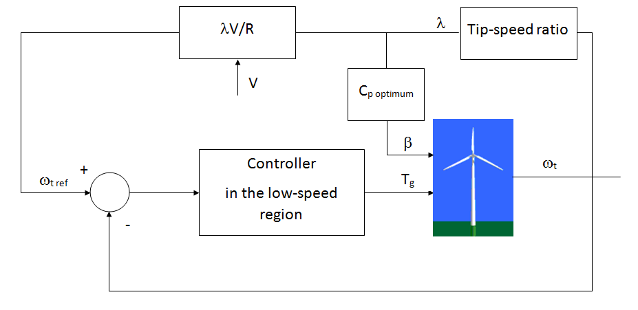
Figure 3: Block diagram in the low-speed region

Fig. 3 presents the monovariable structure of the controller with a low-speed wind. See

• if $t<200$ s then $V_{\text{moy}}=7$ m/s,

• if $t>200$ s, $t<400$ s then $V_{\text{moy}}=8$ m/s,

• if $t>400$ s then $V_{\text{moy}}=9$ m/s,

and Fig. 4. Performances of PI and iP controllers are compared.

IV-A1 iP

The parameters $K_{P}$ and $\alpha$ are given in the Table IV. As explained in Section III, $\tau$ must be chosen quite small.

TABLE IV: iP controller parameters for the weak wind

Variable	Control of $T_{\text{g}}$
$K_{P}$	-0.45
$\alpha$	0.0005
$\tau$	20

Fig. 5 shows the efficiency of the iP controller:

• The turbine angular speed $\omega_{\rm t}$ oscillates around the reference value.

• This reference value varies in function of the wind speed value.

• The blade pitch angle $\beta$ varies between 0 and 2 degrees.

• Blades are positioned to recover the maximum energy.

• The generator torque $T_{\text{g}}$ is limited to $162$ kNm.

IV-A2 PI

For $T_{\text{g}}$, the Ziegler-Nichols method (see, e.g., [24]) yield the coefficients of the PI controller: seeTable V:

TABLE V: PI controller parameters for the weak wind

Variable	Control of $T_{\text{g}}$
$K_{P}$	500
$K_{I}$	10

See Fig. 6 for the results.

IV-A3 Performances comparison of the two controllers

The aim is to maximize the wind energy $P_{\rm t}$. The mean absolute error (MAE) and the corresponding standard deviation for each controller are evaluated for the iP and PI: See Table VI. The mean of the output power, which is calculated between $t=60$s, where the steady state is established, and the final time $t=600$s, is higher with the iP. The iP is thus more efficient.

TABLE VI: MAE and standard deviation comparison for $\omega_{\rm t}$ and $P_{\rm t}$ with an alternating wind in the low-speed region

Controller			iP	PI
Weak wind	$\omega_{\rm t}$ (rad/s)	MAE	0.43	0.61
		standard deviation	0.55	0.70
	$P{\rm t}$ (kW)	MAE	279	278

IV-B Simulation with an alternating wind in the high-speed region

Fig. 7 exhibits the new MIMO control structure with $2$ control and output variables. See Fig. 8 for the wind. There are two operating points:

• if $t<300$ s then $V_{\text{moy}}=16\;$ m/s,

• if $t>300$ s then $V_{\text{moy}}=20\;$ m/s.

IV-B1 iPs

See Table VII for the choice $K_{P}$, $\alpha$ and $\tau$. As depicted by Fig. 9,

• $P_{\rm e}$ remains stable around $P_{\rm rated}$ = 600 kW,

• $\omega_{\rm t}$ remains close to the reference,

• 1. the initial value of $\beta$ is equal to 30 degrees,

  2. then it is approximately equal to 21 degrees until $t=300$s when the steady state is established,

  3. for $t>300$s it fluctuates around 29 degrees when the mean wind speed increases to 20 m/s,

• the value of $T_{g}$ stays around 130 kNm when the steady state is established.

TABLE VII: Model-free control parameters for the strong wind

Variable	Control of $\beta$	Control of $T_{\text{g}}$
$K_{P}$	-4	3
$\alpha$	1	1000
$\tau$	20	20

IV-B2 PIs

See Table VIII for the gains of the two PIs which are again determined via the Ziegler-Nichols method. According to Fig. 10, their performances are poorer.

TABLE VIII: PI controller parameters for the strong wind

Variable	Control of $\beta$	Control of $T_{\text{g}}$
$K_{P}$	-0.006	-0.0003
$K_{I}$	0.52	-0.00026

IV-B3 Performances comparison of the two controllers

The main objective is not to maximize the electrical production but to maintain it close to $P_{\rm rated}$ = 600 kW as shown in Fig. 1. As in Section IV-A3 MAE and standard deviation are reported in Table IX. They confirm the marked superiority of iPs.

Remark 4

The advanges of intelligent controllers with respect to PIDs were already noticed several times. See [31, 32] for two recent most convincing examples.

TABLE IX: MAE and standard deviation comparison for $\omega_{\rm t}$ and $P_{e}$ with an alternating wind in the high-speed region

Controller			Intelligent P	Classical PI
Strong wind	$\omega_{\rm t}$ (rad/s)	mean	0.33	0.38
		standard deviation	0.39	0.45
	$P_{e}$ (kW)	mean	32	48
		standard deviation	38	56

IV-C Fault accommodation and iP

Simulate, as proposed by [33], an actuator fault, occurring at $t=300$ s with a wind speed equal to $16$ m/s, with respect to the electromagnetic torque $T_{\text{g}}$:

• a loss of efficiency equal to 15%, i.e.,

  $$T_{{\text{g\ actuator}}}=0.85\times T_{\rm g}$$

  where $T_{\text{g\ actuator}}$ is the control applied to the turbine;

• a bias fault equal to 50 kNm, i.e.,

  $$T_{\text{g\ actuator}}=T_{\rm g}-50$$

IV-C1 Loss of efficiency

Fig. 11 depicts the good results for the iP. Let us emphasize that our setting is modifying $\beta$.

IV-C2 Bias fault

Fig. 12 exhibits similar results to those in Section IV-C1.

V Conclusion

The promising simulations depicted here need of course to be confirmed, especially via some concrete plants. The behavior of our control strategy with respect to the unavoidable vibrations (see, e.g., [34, 35]) should of course be clarified. For a better energy management, some forecasting of the wind power is crucial. It would be rewarding to extend the time series techniques for photovoltaic energy [36], which bears some similarity with MFC.

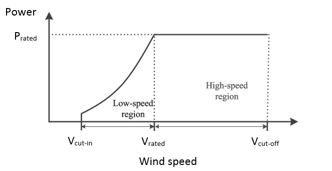
Figure 1: Operating range [7]

Figure 4: Alternating wind in the low-speed region

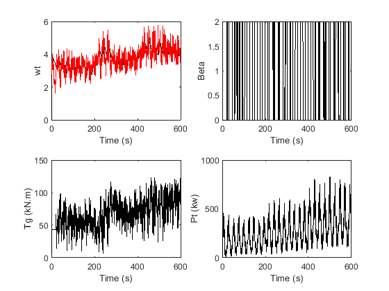
Figure 5: Control of $\omega_{\rm t}$ and $P_{e}$ with an alternating wind in the low-speed region (iP controller)

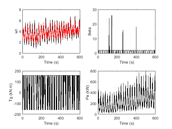
Figure 6: Control of $\omega_{\rm t}$ and $P_{e}$ with alternating wind in the low-speed region (PI controller)

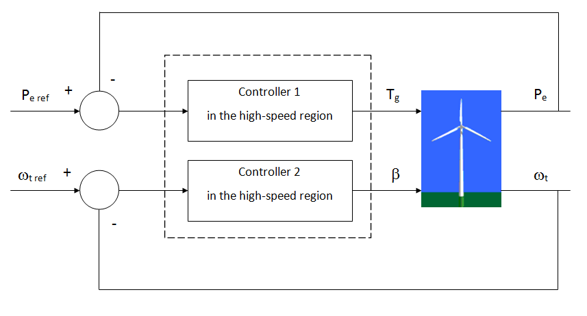
Figure 7: Block diagram in the high-speed region

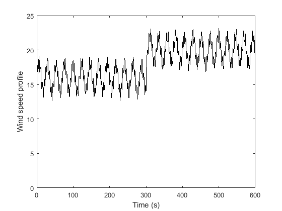
Figure 8: Alternating wind in the high-speed region

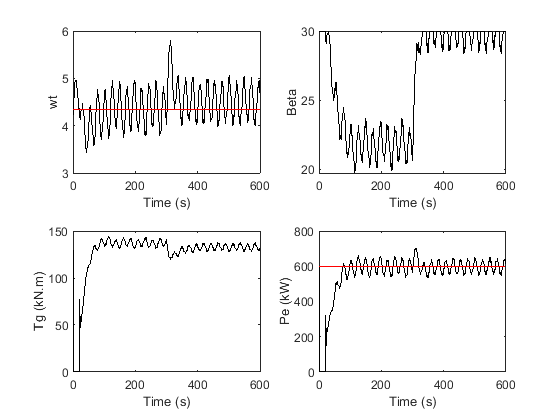
Figure 9: Control of $\omega_{\rm t}$ and $P_{e}$ with alternating wind in the high-speed region (iP controller)

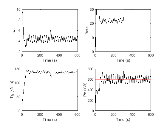
Figure 10: Control of $\omega_{\rm t}$ and $P_{e}$ with alternating wind in the high-speed region (PI controller)

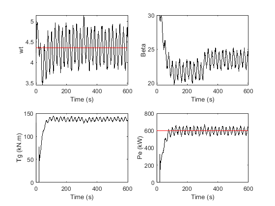
Figure 11: Fault accomodation with iP (loss of efficiency)

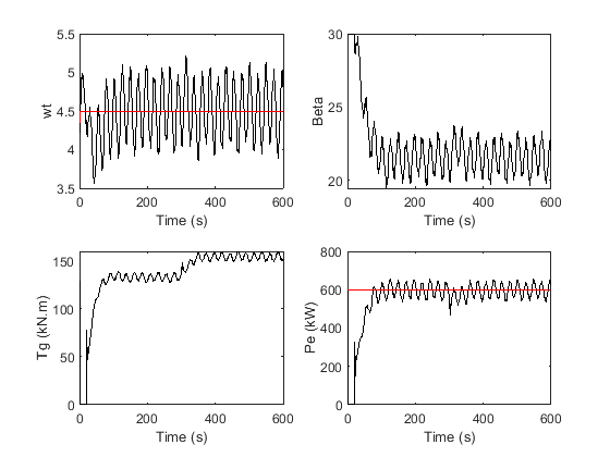
Figure 12: Fault accommodation with iP (bias fault)

References

- [1] N. Luo, Y. Vidal, L. Acho, Wind Turbine Control and Monitoring, Springer, 2014.
- [2] J.G. Njiri, D. Söffker, “State-of-the-art in wind turbine control: Trends and challenges,” Renew. Sustain. Energy Reviews, vol. 60, 2016, pp. 377–393.
- [3] E.J. Novaes Menezes, A.M. Araújo, N.S. Bouchonneau da Silva, “A review on wind turbine control and its associated methods,” J. Clean. Prod., vol. 174, 2018, pp. 945–953.
- [4] W.H. Lio, Blade-Pitch Control for Wind Turbine Load Reductions, Springer, 2018.
- [5] M. Ghanavati, A. Chakravarthy, “PDE-based modeling and control for power generation management of wind farms,” IEEE Trans. Sustain. Energ., vol. 10, 2019, pp. 2104–2113.
- [6] S. A. De La Salle, D. Reardon, W. E. Leithead, M. J. Grimble, “Review of wind turbine control,” Int. J. Contr., vol. 52, 1990, pp. 1295–1310.
- [7] W. Meng, Y. Ying, Y. Sun, Z. Yang, Y. Sun, “Adaptive Power Capture Control of Variable-Speed Wind Energy Conversion Systems With Guaranteed Transient and Steady-State Performance,” IEEE Trans. Ener. Conver., vol. 28, 2013, pp. 716–725.
- [8] K. Åstrom, T. Hägglund, Advanced PID Control, Instrument Soc. Amer., 2006.
- [9] A. O’Dwyer, Handbook of PI and PID Controller Tuning Rules (3rd ed.), Imperial College Press, 2009.
- [10] H. Habibi, H. R. Nohooji, I. Howard, “Adaptive PID control of wind turbines for power regulation with unknown control direction and actuator faults,” IEEE Access, vol. 6, 2018, pp. 37464–37479.
- [11] M. Mirzaei, C. Tibaldi, M.H. Hansen, “PI controller design of a wind turbine: evaluation of the pole-placement method and tuning using constrained optimization,” J. Phys. Conf. Ser., vol. 753, 2016.
- [12] Y. Ren, L. Li, J. Brindley, L. Jiang, “Nonlinear PI control for variable pitch wind turbine,” Contr. Engin. Pract., vol. 50, 2016, pp. 84–94.
- [13] M. Fliess, C. Join, “Model-free control,” Int. J. Contr., vol. 86, 2013, pp. 2228–2252.
- [14] O.Bara, M.Fliess, C. Join, J. Day, S.M. Djouadi, “Toward a model-free feedback control synthesis for treating acute inflammation,” J. Theoret. Biology, vol. 448, 2018, pp. 26-37.
-
[15]
M. Fliess, C. Join, “Machine learning and control engineering: The model-free case,” Future Techno. Conf., Vancouver, 2020.
https://hal.archives-ouvertes.fr/hal-02851119/en/ - [16] S. Li, H. Wang, Y. Tian, A. Aitouch, J. Klein, “Direct power control of DFIG wind turbine systems based on an intelligent proportional-integral sliding mode control,” ISA Transactions, vol. 64, 2016, pp. 431–439.
- [17] A. Ardjal, M. Bettayeb, R. Mansouri, A. Mehiri, “Model-free intelligent proportional-integral control of a wind turbine for MPPT,” Int. Conf. Elec. Comput. Techno. App., Aurak (UAE), 2017.
- [18] M. Abouheaf, W. Gueaieb, A. Sharaf, “Model-free adaptive learning control scheme for wind turbines with doubly fed induction generators,” IET Renew. Power Generat., vol. 12, 2018, pp. 1659–1667.
- [19] C. Join, G. Robert, M. Fliess, “Vers une commande sans modèle pour aménagements hydroélectriques en cascade,” 6e Conf. Internet. Francoph. Automat., Nancy, 2010. https://hal.inria.fr/inria-00460912/en/
- [20] S. Heier, “Grid Integration of Wind Energy Conversion Systems,” John Wiley & Sons Ltd, vol. 20, 1998, pp. 521–527.
- [21] K. Kyung-Hyun, V. Tan Luong, L. Dong-Choon, S. Seung-Ho, K. Eel-Hwan, “Maximum Output Power Tracking Control in Variable-Speed Wind Turbine Systems Considering Rotor Inertial Power,” IEEE Transactions on Industrial Electronics, vol. 60(8), 2013, pp. 3207–3217.
- [22] B. Boukhezzar, L. Lupu, H. Siguerdidjane, M. Hand, “Multivariable control strategy for variable speed, variable pitch wind turbines,” Renewable Energy, vol. 32, 2007, pp. 1273–1287.
- [23] R. Melicio, V.M.F. Mendes, J.P.S. Catalao, “Full-Power Converter Wind Turbines with Permanent Magnet Generator: Modeling, Control and Simulation,” Proc. IEEE Inte. Elect. Mach. Drives, Miami, 2009.
- [24] G.F. Franklin, J.D. Powell, A. Emami-Naeini, Feedback Control of Dynamic Systems (8th ed.), Pearson, 2019.
- [25] A. Rudin, Functional Analysis (2nd ed.), McGraw-Hill, 1991.
- [26] K. Yosida, Operational Calculus (translated from the Japanese), Springer, 1984.
- [27] M. Fliess, “Analyse non standard du bruit,” C.R. Acad. Sci. Paris Ser. I, vol. 342, 2006, pp. 797–802.
-
[28]
C. Join, F. Chaxel, M. Fliess, “Intelligent controllers on cheap and small programmable devices,” 2nd Int. Conf. Control Fault-Tolerant Syst., Nice, 2013.
https://hal.archives-ouvertes.fr/hal-00845795/en/ - [29] F. Lafont, J.-F. Balmat, N. Pessel, M. Fliess, “A model-free control strategy for an experimental greenhouse with an application to fault accommodation,” Comput. Electron. Agricult., vol. 110, 2015, pp. 139–149.
- [30] Y. Wang, H. Li, R. Liu, L. Yang, X. Wang, X., “Modulated model-free predictive control with minimum switching losses for PMSM drive system,” IEEE Access, vol. 8, 2020, pp. 20942–20953.
-
[31]
J. Villagra, C. Join, R. Haber, M. Fliess, “Model-free control for machine tools,” 21st IFAC World Congress, Berlin, 2020.
https://hal.archives-ouvertes.fr/hal-02568336/en/ -
[32]
M. Clouatre, M. Thitsa, M. Fliess, C. Join, “A robust but easily implementable remote control for quadrotors: Experimental acrobatic flight tests,” 9th Int. Conf. Advanc. Techno., Istanbul, 2020.
https://hal.archives-ouvertes.fr/hal-02910179/en/ - [33] H. Badihi, Y. Zhang, H. Hong, “Wind turbine fault diagnosis and fault-tolerant torque load control against actuator faults,” IEEE Trans. Contr. Syst. Techno., vol. 23, 2015, pp. 1351–1372.
- [34] W. He, S.S. Ge, “Vibration control of a nonuniform wind turbine tower via disturbance observer,” IEEE/ASME Trans. Mechatron.., Vol. 20, 2014, pp. 237–244.
- [35] S. Gao, J. Liu, “Adaptive fault-tolerant vibration control of a wind turbine blade with actuator stuck,” Int. J. Contr., vol. 93, 2020, pp. 713–724.
- [36] M. Fliess, C. Join, C. Voyant, “Prediction bands for solar energy: New short-term time series forecasting techniques,” Solar Energy, vol. 166, 2018, pp. 519–528.