When deep learning models on GPU can be accelerated by taking advantage of unstructured sparsity

Abstract

This paper is focused on the improvement of the efficiency of sparse convolutional neural networks (CNNs) layers on graphic processing units (GPU). The Nvidia deep neural network (cuDnn) library provides one of the most effective implementations of deep learning (DL) algorithms for GPUs. GPUs are the most efficient and commonly used accelerators for deep learning computations. Modern CNN models need megabytes of coefficients and millions of MAC operations to perform convolution. One of the most common techniques for compressing CNN models is weight pruning and quantization. There are two main types of pruning: structural (based on removing whole weight kernels) and non-structural (removing individual weights). The first enables much easier acceleration on many type of accelerators, but with this type it is difficult to achieve a sparsity level and accuracy as high as that obtained with the second type. Non-structural pruning with retraining can generate a matrix-weight up to $\sim 90\%$ or more of sparsity in some deep CNN models. This work shows when it is worth using a direct sparse operation to speed-up the calculation of the convolution layers. In the next stage the linear and non-linear quantization is performed for further cycles and memory reduction. This work presents the impact of using reduced precision on time efficiency.

Keywords CNN, GPU, pruning, cuDnn, Cublas, reduced precision

1 Introduction

Deep convolutional neural networks (CNNs) achieve outstanding results in various artificial intelligence tasks including image classification [1][2], object detection [3], semantic segmentation and natural language processing [4][5][6]. Recent CNN neutral networks consist of dozens of convolution layers and a few fully connected layers. Neural networks for conducting the training process on large benchmark datasets need different accelerators such as multi-core processors, GPGPUs or other dedicated hardware accelerators. Over the years, scientists have been looking for methods to accelerate the calculations of the convolution operation. The direct convolution algorithm to perform convolutions requires $N^{2}$ multiplications and N(N-1) additions where N is the size of the input. For the same input the Fast Fourier Transform (FFT) method reduces operation complexity to O(N$log_{2}$(N)) [7]. The Winograd algorithm is suitable for small fixed-size kernels and requires 2.25 times fewer multiplications than direct convolution [8]. The convolution operation can be realised by matrix-multiplication [9], especially on the GPGPU which is highly tuned for performing this operation [10]. The GPGPU remains one of the most efficient and commonly used hardware accelerators. The NVIDIA deep neural network library (cuDNN) performs convolution with different algorithms (Winograd, FFT, GEMM) depending upon filter size, batch size and data representation. Apart from choosing different algorithms for speeding up convolution there are some other methods based on complexity and memory footprint reduction. Some CNN models for image processing or natural language processing can be heavily pruned. The effect of this process is that they very often contain zero values more than 80% of weights. Depending upon the level of sparsity, it can be worth performing the convolution through the application of the direct sparse convolution method proposed by Chen [11]. The paper concentrates on two aspects. The first is about methods for complexity reduction. It explains pruning and quantization methodologies and theirs results. The second is focused on investigating when it is worth using sparse operations, instead of using dedicated NVIDIA libraries to perform the convolution layer on the GPGPU. As the main optimization strategy we propose the introduction of a unified sparse level for each of the output channels in each convolutional layer. The other optimization strategy is determining the most optimal number of thread blocks for each convolutional layer separately. The presented approach is optimized towards the optimal arrangement of the data in order to obtain acceleration with the direct convolution approach using the sparse format. These strategies are crucial for achieving peak performance. This work shows real examples of models where it is possible to obtain the appropriate level of sparsity so that acceleration using the presented algorithm vs cuDnn could be possible. These examples are well known CNN models used on smaller and less complex data sets. The high sparsity levels were obtained by the presented pruning approach. Apart from achieving a high sparsity and compression ratio, the accuracy levels were also improved. Finally, the impact on time efficiency of using half precision (FP-16) in a direct sparse convolution is explored. It is compared with cuDnn, where for 16-bit data representation, NVIDIA Tensor Cores specialised arithmetic units are used. In the presented work quantization is used in two variants: after pruning in the training process and on a pretrained model. Both linear and nonlinear approaches of quantization were applied. To our knowledge, this is the first work that shows the acceleration of the unstructured sparsity of weights compared to the dense approach using real models.

2 Related work

Convolution complexity and efficiency optimization have recently become quite popular research subject. Jordá et al. [12] present the way in which the cuDnn library calculates convolution layers dependent upon parameter configurations and data representation. Lavin et al. [8] introduces Winograd convolution implementation which is based on minimal filtering algorithm. This approach for a small filter and batch size was 2.26 times faster than the previous version of cuDnn. Adámek et al. [7] proposes an FFT based convolution on GPGPU by the shared memory implementation of the overlap-and-save method, and for certain sizes, a 30% speed increase was achieved in comparison to cuDnn. The direct sparse convolutions method was proposed in [13]. The authors used the CSR format to store the weights and perform the convolution operation by use of the sparse matrix multiplication. This approach achieved 3.1-7.3 times speed increase comparison to dense convolution in the AlexNet model, on Intel Atom, Xeon and Xeon Phi processors. Lu et al. [14] proposed FPGA’s sparse convolution implementation which in VGG16 is almost three times faster than FPGA’s dense implementation. The same type of convolution was applied on the GPU in [11], where the speed increase for AlexNet [15], GoogleLeNet [16] and ResNet [17] models were respectively 1.74, 1.34 and 1.43 times that of the GEMM implementation in the CUBLAS library. Zhu et al. [18] used sparse matrix operation in order to perform recurrent neural networks (RNN), where the data format of sparse persistent RNN is represented by the $\langle index,value\rangle$ pairs. The authors have proposed several optimization strategies for GPU implementation such as wide memory loads and bank-aware weight layouts. This approach for a hidden layer of size 1782 and density of 10% allows the following speed increases to be achieved: 7.3 times that of dense GEMM (cuDnn), 3.4 times that of sparse GEMM (cuSparse) and 1.8 times compared to dense persistent implementation (cuDnn). An important role in sparse convolution is played by weight pruning, which can produce a number of zero weights . Information about the level of weight sparsity can be used after the pruning step in order to decide if it is worth running direct sparse implementation or cuDnn. The paper shows models and data sets on which it is possible to achieve a level of sparsity which can provide a better level of efficiency than cuDnn by using direct sparse convolution. In other research [19], the authors prove that retraining with pruning can reduce the drop in accuracy caused by removing unimportant weights. Pruning is one of the most popular solutions when it comes to memory compression and the acceleration of deep learning models [19], [20], [21]. When it comes to accelerating models with pruning, dedicated accelerators are very often built (eg. based on FPGA) that can use unstructured pruning. Recently, there has been a lot of research on pruning. Some of the most popular approaches of pruning methods which incorporate retraining are: pruning without retraining with local search heuristics [19],[22], lottery ticket [20], movement pruning [21] and [23]. In most of the mentioned works there is no real use of the results obtained from unstructured sparsity in the GPU. Many modern hardware accelerators support reduce bit precision arithmetic. Quantization is the next step by which it is possible to reduce workload and memory further. Many quantization approaches were applied for deep learning [24] [25] [26] using linear or nonlinear quantization, regularization modifications, clustering [27] and other techniques [22].

3 Convolutional neutral networks

The typical convolutional layer in a feed-forward procedure calculates the convolution of the inputs which is represented by a batch of N samples (images, time series etc.) with C channels and size H$\times$W, with a set of K filters with C channels and size R$\times$S. The output product of convolution contains K matrices with size E$\times$F, where $E=\frac{H+2*padding-R}{stride}+1$ and $F=\frac{W+2*padding-S}{stride}+1$. The set of parameters of a single convolution layer is a 4D array called a tensor. When the kernel is marked as W and the input is marked as I the convolution of a single layer is given by the formula:

$$Out_{n,i,j,k}=\sum_{c=0}^{C-1}\sum_{r=0}^{R-1}\sum_{s=0}^{S-1}W_{k,c,r,s}I_{n,c,i+r,j+s}$$ (1)

The result of the above formula is added to the bias parameter b and the activation function is then applied [28]. The convolution layers are the most time-consuming operation in the CNN flow. For this reason, only these layers have been subjected to an acceleration in this paper. In our experiments the VGG-16 [29], CNN-non-static [4] some 1x1 layers from ResNet [17] and DenseNet [30] models were used as a benchmarks.

4 Convolution algorithms on the GPGPU

In order to perform forward convolution the cuDnn library always chooses the most effective algorithm, depending upon input, filter, batch size and data format. The graphics processing units (GPUs) are very effective particularly for accelerating large matrix products such as matrix-matrix multiplication and element-wise multiplication. For this reason, the most productive algorithms for performing convolution on GPGPUs firstly transforms the data to a form which allows performing the convolution through the application of these operations. The first most commonly used algorithm is general matrix multiply (GEMM). This method transforms the input and the filters into two matrices. Convolution is performed by the scalar product of the single row and the single column which is repeated for each input’s column and all rows from transposed filters. This method is used when data are represented at half precision, in 1D, a 1$\times$1 convolution and when the number of channels is relatively small, which usually takes place for the first layers of most CNN’s architecture. The second method is based on the Fast Fourier Transform (FFT). This method for transforming the convolution of two signals in one domain (e.g. time) is equivalent to the point-wise multiplication of their Fourier transform in the other domain (e.g. the frequent domain). After calculation the inverse Fast Fourier Transform is requested in order to return back to the time domain. In theory, FFT convolution is the most effective way to perform convolution for large filters like 5x5. Based on VGG-16 architecture, the cuDnn uses this method to perform convolution in the case of the input size being smaller than or equal to 58$\times$58 (from the sixth layer) and for a batch size higher than 32. The last method to perform convolution on GPGPU is Winograd. This method is based on the Chinese reminder theory (CRT)[31]. Thanks to introducing some transformations there is a reduction in the number of multiplications and an immediate increase in the number of required additions, which results in a faster computation.

5 Pruning

Very often, many deep learning models have a lot of redundant weights. Research in the exploration of pruning techniques has been recently showed that many cases of deep learning architecture can be compressed with high ratios. Several methodologies have already been tried. The most popular techniques are for example pruning with or without retraining [19], incremental pruning or pruning with a constant sparsity [20], pruning with constant mask or dynamic, gradient-based pruning [21]. The work focuses on the application of popular deep learning models to CIFAR100 and CIFAR10. In less complex data sets like CIFAR100 with a reduced number of classes (smaller than Imagenet) there is a higher probability of obtaining such sparsity levels that can give a faster solution than cuDnn. In addition, the work shows that not only such models can be accelerated on data sets of reduced complexity (e.g. with a smaller number of classes) but using the pruning approach, their accuracy can be significantly increase.

5.1 Pruning approach

The proposed pruning method is based on retraining. Pruning with retraining guarantees much better final sparsities. Algorithm 1 incorporates evolutionary techniques and rewinding during its execution. It makes it possible to return to the values of nonzero weights which were before given iteration. The input parameters are:

• $acc\_threshold$ - threshold for accuracy acceptable accuracy changes

• $iter\_nr$ - number of iterations of the algorithm

• $batch\_nr$ - number of batches after which pruning configuration can be changed

• $pool\_size$ - number of solutions in a population

The algorithm starts from scratch with random initial weights and generates a pool of solutions (subnetworks) with random initial sparsities (line 1). In each iteration some subsets of layers are chosen for further pruning. This step helps to gather statistics about layer sensitivity and diagnoses which layer may be blocking learning. The batch training is then performed (it can be the whole epoch, it depends upon the algorithm settings).

0:  $acc\_threshold,iter\_nr,batch\_nr,pool\_size$

1:  $generate\_pool\_of\_solutions$

2:  for $i<iter\_nr$ do

3:     $choose\_subnetwork\_from\_pool$

4:     $choose\_layers\_in\_model$

5:     $train\_batches$

6:     $compute\_grad\_statistics$

7:     $compute\_accuracy$

8:     if $improvement>acc\_threshold$ then

9:        $write\_to\_pool\_if\_good\_enough$

10:        $increment\_mask$

11:     else

12:        $mutation\_or\_crossover$

13:        $rewinding$

14:     end if

15:     $alpha=check\_weights\_migration()$

16:     $update\_sensitivity$

17:     if $stagnation$ then

18:        $differentiate\_solutions\_in\_pool$

19:     end if

20:  end for

Algorithm 1 Pruning - main scheme approach

After the batch training gradient analysis is performed and the accuracy is measured on a validation set (line 6 and 7). The current solution is compared with others from the pool. If it is good enough it is written to the population set and its mask (sparsity) is incremented (line 9). The mask in the presented algorithm is a dynamic structure which indicates which weights should be pruned. The mask is recomputed after each batch training (see eqs. 2 and 3). The $wg_{n,i,j,k}$ coefficient for each weight is computed based on its absolute value and its current gradient value. $Alpha$ parameters define how important these factors are.

$$wg_{n,i,j,k}=alpha*grad_{n,i,j,k}+(1-alpha)*abs(w_{n,i,j,k})$$ (2)

$$mask_{n,i,j,k}=1\;if\;wg_{n,i,j,k}\in max(wg,sparsity)\;else\;0$$ (3)

The mask increase is set on the basis of the sensitivity of pruned layers. If the progress in training the model is not satisfactory (line 8), rewinding and mutation or crossover is performed. Mutation is just a random sparsity change in the given layers. Crossover takes two random parents from the population and exchange theirs sparsity numbers in randomly chosen layers.

$$w_{n,i,j,k}=w_{n,i,j,k}*mask_{n,i,j,k}$$ (4)

In the next steps the $alpha$ parameter is computed on the basis of a weights migration statistics (from and into the mask). The sensitivity of the layers is updated, which indicates how the process of pruning specific layers affects the accuracy level. The last step helps to avoid stagnation in the algorithm. The population is divided into a specific number of clusters and only some constant representatives of each cluster stay in the population.

6 Quantization

After the process of network distillation by the pruning process quantization can be performed as the next step of reducing model complexity. Quantization is the procedure of constraining values from a continuous set or more dense domain to a relatively discrete set. It is possible to define a general mapping from a set of floating-point data $x\in{\mathcal{S}}$ to fixed-point $q$ as follows (assuming signed representation):

$$q_{\textit{fxp}}={\mathcal{Q}}(x_{\textit{flp}})=\mu+\sigma\cdot\textit{round}(\sigma^{-1}\cdot(x-\mu)).$$ (5)

In our case $\mu=0$ and $\sigma=2^{-{\bf frac\_bits}}$ where

$${\bf int\_bits}=\textit{ceil}(\log_{2}(\max_{x\in{\mathcal{S}}}|x|))$$ (6)

and ${\bf frac\_bits}={\bf total\_bits}-{\bf int\_bits}-1$. The scaling factor $\sigma$ is essentially just a shift up or down. A drawback is that a great deal of precision may be lost if the distribution of the data set ${\mathcal{S}}$ is skewed by a large mean. Yet another approach can define the number of integer and fractional bits to represent regions of a distribution that will represent a large percentage of the range. In these cases, there will be saturation of a small percentage of the data, such as outliers, through the quantization procedure which may or may not significantly affect the accuracy. To determine the effects of saturation one can experiment with different saturation levels. Therefore histogram analysis is used to analyze outliers and set the best levels of saturation for activation of quantization.

The eq. 5 can be adapted to mapping floating numbers to integers values:

$$q_{\textit{int}}={\mathcal{Q}}(x_{\textit{flp}})=ceil((x-\mu)/((max(X)-min(X))\cdot\sigma^{-1}))$$ (7)

The $\mu$ parameter can be set to $min(X)$ ($X$ is an input set of values to be quantized) or can have a value of zero. In the first case it is known as an asymmetric integer quantization (e.g. used in TensorFlow framework), in the second, it is called symmetric. In this work fixed point was applied. To compare linear quantization results, a nonlinear technique based on clustering was implemented. This approach assigns weight values for given layer to a given number of centroids eq. 8. After that each weight is assigned to a cluster centroid which it belongs to eq. 9. The codebook of values is created. During inference/forward pass each original value is mapped to its reduced centroid representation (16 or 8 bit). This approach gives additional memory compression.

$$C,W_{c}=clustering(W)$$ (8)

$$W_{c}=\{\forall w_{c}\in W_{c},\exists c_{i}\in C:w_{c}=c_{i}\}$$ (9)

7 Building CSR weight format

After the training process incorporated with incremental pruning, the model contains a set of weights with values set to zero. From the point of view of this paper, the most important element of pruning is the extracting information the lowest sparsity level occurs with the K output channels. This information is used to unify the sparsity level for each output channel. This procedure is significant for GPU implementation, where the execution time is depends upon the output channel with the lowest sparsity (see Section 8). Having a standardized sparsity level, pruned weights enables the compressed sparse row (CSR) format for each convolution layer to be built. To represent the matrix, the CSR format needs to build three arrays:

• Values - these contains only non-zero elements.

• Coldix - on each position contains a offset for the value on equivalent position in the value array. Park et al. [32], proposed pre-computed value in the coldix matrix to store indexes from the input array which will be used to perform convolution. Thanks to this, there is no necessity to calculate these indexes during convolution which decrease calculation time.

• Rowptr - rowptr[i] is the point to the first non-zero element of the ith output channel. Note that the result of rowptr[i+1] - rowptr[i] is the number of non-zero elements in the ith output channel. In our approach, this number is the same for each output channel thanks to the aforementioned standardized sparse level and we call this the $sparse\_level$. The only modification which must be done to avoid calculating the sparsity level separately for each output channel is mark some zero value as "non-zero" and during building, the CSR format treats them as normal value. This operation does not change the result and needs extra-memory. However, having the same sparsity for each output channel determines that each warp on the GPGPU has the same number of iterations, which is known before running the CUDA kernel which leads to the kernel’s faster execution. These special "non-zero" values are chosen to not excessively jump thorough memory this mean there are choose zeros with side-by-side indices to guarantee contiguous direct memory access .

8 Convolution operation using a sparse operation on GPGPU

To perform convolution by usage of a sparse operation the direct sparse convolution [32] was used. In parallel implementation we use an approach proposed by [11]. The input data are stored in NCHW format (batch size, channel, height, width). The weights are stored in the CSR format where coldix and value arrays are loaded into shared memory. Each single thread block, calculates one output channel so for one input vector the total number of thread blocks is equal to the number of output channels. In our approach, we optimize the number of input vectors from the input batch, which will be handled by this number of blocks and is denoted as $subBatchSize$. As a result, the total number of thread blocks is equal to $\frac{batchSize*numberOfOutputChannel}{subBatchSize}$ which is presented by Fig. 1.

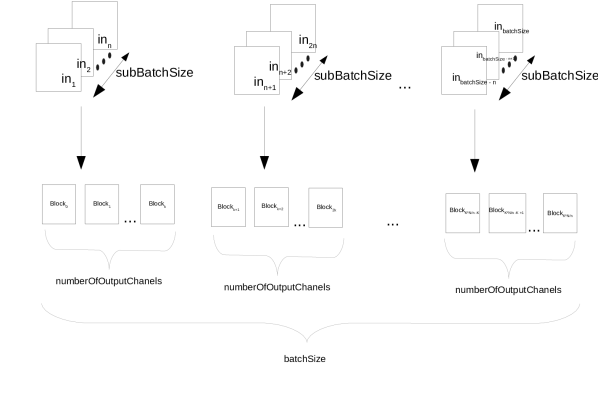
Figure 1: The total number of thread’s block using to perform convolution for a single layer

As it turns out, this number depends on the layer size and belongs to {2, 4, 8} (see section 9). This optimal number is not the same for each type of layer due to the cache limitation and when this particular memory is missed, data are put into global memory which is very slow. For this reason, in this paper this number was experimentally fixed for each layer. During the calculation of the convolution, non-zero values from the values array and pre-calculated indices of the input vector from the coldix array are loaded from shared memory into the thread local memory and it is reused for $subBatchSize$ input vectors. This procedure enables maximum limitation of the reading from shared memory. Similar to the weights and indexes values, the partial sums are stored in registers and are copied to global memory after calculations. The number of threads used for the calculation of one output channel for one vector is determined by the output size of convolution. Each single thread is responsible for calculating one single output value by multiplication with the weight with corresponding input value, accumulating the partial sum and writing the final result to the global memory as is shown in Fig. 2. The total number of working threads in a single threads block is determined by the sparsity level which in our approach is the same for each output channel and is equal to sparsity of channel with minimum value (see Section 7). In the version of the implementation where each channel has different sparsity the execution time was longest $\sim 28\%$ for VGG-16 $3x3$ and $1x1$ convolution type and $\sim 26\%$ in the case of both convolution layers from CNN-non static. As an improvements both weights and input feature maps are marked as constant in order to hold them in the L2 cache, and coalesced memory access is provided. This convolution function is chosen for the cuDnn flow and performs convolution instead of the cuDnn function in the case of specific sparsity level (higher than $\sim$ 90% for vgg-16 and 1x1 convolution, and more than $\sim$78% for CNN-non static) and this is achieved only for some layers, as is shown in the next sections. The greatest acceleration of direct sparse convolution over the cuDnn was achieved for the 1D convolution. In this case, the input data are in the shape of a vector; therefore to preform convolution by usage of the direct sparse method, less memory jumps are needed than with 2D convolution. Besides sparsity we are checking how precision reduction can accelerate the calculation of convolution in sparse implementation and with usage of dedicated libraries. In order to achieve this, data are transformed from float to half type for both weights (the value array) and input data. Cuda-Math-Api is used in order to perform calculations with half the precision on the GPU. Cuda-Math-Api provides transformations and mathematical functions for half type. As described in [23] and [22] the 16-bit half precision is sufficient to to keep the CNN models accuracy on the same level.

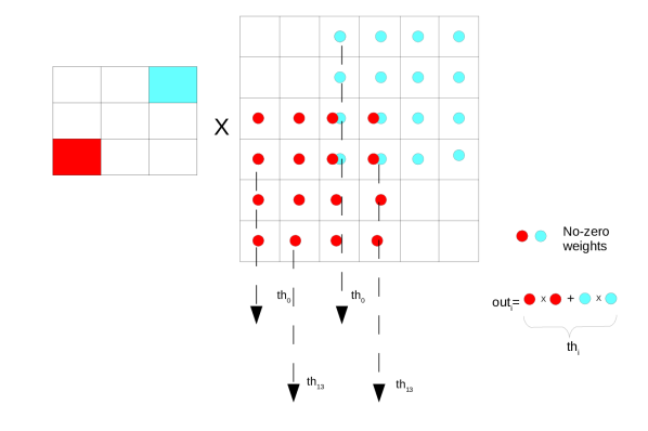
Figure 2: Calculating convolution using a sparse operation

	Accuracy	Weighted sparsity
VGG16 dense	90.01	0.0
VGG16 sparse	92.5	96.2

Table 1: Table with VGG16 pruning results on CIFAR10.

	Accuracy	Weighted sparsity
VGG16 dense	64.99	0.0
VGG16 sparse	68.31	92.2

Table 2: Table with VGG16 pruning results on CIFAR100.

	Accuracy
VGG16 sparse 4b/16b	68.2
VGG16 sparse 16b/16b	68.3

Table 3: Table with VGG16 quantization results on CIFAR100.

	Accuracy	Weighted sparsity
Resnet50 dense	92.3	0.0
Resnet50 sparse	94.1	97.14

Table 4: Table with Resnet50 pruning results on CIFAR10.

	Accuracy	Weighted sparsity
Resnet50 dense	67.06	0.0
Resnet50 sparse	78.23	90.14

Table 5: Table with Resnet50 pruning results on CIFAR100.

	Accuracy
Resnet50 sparse 4b/16b	93.8
Resnet50 sparse 16b/16b	94.0

Table 6: Table with Resnet50 quantization results on CIFAR100.

	Accuracy	Weighted sparsity
DenseNet dense	82.0	0.0
DenseNet sparse	84.0	89.5

Table 7: Table with DenseNet pruning results on CIFAR100.

	Accuracy
DenseNet sparse 4b/16b	83.5
DenseNet sparse 16b/16b	84.1

Table 8: Table with DenseNet quantization results on CIFAR100.

0:  $sparsity\_thresholds\_for\_specific\_layers$

1:  $run\_pruning$

2:  $quantization$

3:  $layers\_efficiency\_comparing(cudnn,direct)$

4:  $network\_configuration$

Algorithm 2 Main scheme applying reduced bit format and unstructured sparsity in GPU

The described process of pruning produces layers with certain number of zero weights. Then these layers are mapped to direct sparse implementation. At the end quantization is applied. Finally efficiency of layers with reduced number of weights and bit format is compared with CuDnn. Based on these results network is configured to be partially run with direct sparse approach. The whole process is described in alg. 2.

9 Results

In tables 1, 2, 4 and 5 the accuracy and level of sparsity are described which were achieved by pruning algorithm on VGG16 and Resnet50 on CIFAR10 and CIFAR100. The dense models are the baseline models. We can see that apart from high sparsity and huge memory reduction the accuracy is increased. In case of Resnet50 it is worth to note that achieved pruned version is one of the smallest model in TOP40 models in the CIFAR100 ranking [33]. The results were achieved by running 200 epochs of the training process. In results only weighted sparsity are given. In case of Resnet50 about half of all layers are above speedup threshold (>90%) and in VGG16 all except the first layer (fig. 3 and 4). In tables 3 and 6 the results of quantization approaches are presented. The linear 16 bit (half precision both for weights and activations - 16b/16b) quantization and cluster based 4 bit quantization were performed (weights are mapped to 16 centroids, each centroid represented in 16 bit format). The quanization was run on a pretrained and pruned models. It is worth noting that in all cases no drop in accuracy was observed (<0.5%). In tables 7 and 8 results for DenseNet model are described for the same pruning and quantization configurations. Improvement in accuracy after pruning was observed and slight drop after quantization.

Convolution size (CHWK)	Escoin time - float	cuDnn time - float \conv algorithm	Escoin time - half	cuDnn time -half \conv algorithm
3x224x224x64	2.48	2.82\GEMM	2.21	2.71\GEMM
64x224x224x64	60.73	19.07\WINOGRAD	27.08	31.82\GEMM
64x112x112x128	16.45	10.56\WINOGRAD	8.87	9.48\GEMM
128x112x112x128	28.11	17.28\WINOGRAD	17.31	15.88\GEMM
128x56x56x256	13.61	9.21\FFT-TILING	8.74	7.81\GEMM
256x56x56x256	23.72	14.27\FFT-TILING	15.83	16.09\GEMM
256x28x28x512	9.34	6.72\FFT-TILING	6.07	7.86\GEMM
512x28x28x512	16.06	15.02\FFT-TILING	14.01	16.82\GEMM
512x14x14x512	4.31	4.84\FFT-TILING	4.18	4.66\GEMM

Table 9: Time results [ms] for VGG-16 (sparsity $\sim 90\%$)

Layer name	Sparsity [%]	subBatchSize (optimal)	Escoin -float	Cudnn -float	Escoin -half	Cudnn -half
densenet121/ dense_block_3/ dense_layer24	87,5	8	0.69	0.73	0.62	0.68
densenet_121/ dense_block_3/ dense_layer_24	91	8	0.46	0.73	0.41	0.68
densenet161/ dense_block_4/ dense_layer_16	91	4	2.43	2.56	2.37	2.49
densenet161/ dense_block_3/ dense_leayer_16	93	4	1.81	2.56	1.75	2.49

Table 10: Time result [ms] for given layer from DenseNet model for 1x1 convolution

Data type	CUDNN Time	Escoin time
float	0.35	0.32
half	0.30	0.27

Table 11: Time results [ms] for ResNet. 256 filters 1x1x64 (sparsity $\sim 90\%$)

Data type	CUDNN Time	Escoin time
float	0.37	0.31
half	0.29	0.24

Table 12: Time results [ms] for ResNet. 64 filters 1x1x256 (sparsity $\sim 90\%$)

Data type	CUDNN Time	Escoin time for given sparsity
		77%	83%	87,5%
float	0.192	0.176	0.126	0.102
half	0.161	0.145	0.097	0.069

Table 13: Time results [ms] for CNN-non-static for input 300x64. kernel size 2

Data type	CUDNN Time	Escoin time for given sparsity
		77%	83%	87,5%
float	0.231	0.236	0.188	0.135
half	0.204	0.182	0.148	0.103

Table 14: CNN-non-static for input 300x64. kernel size 3

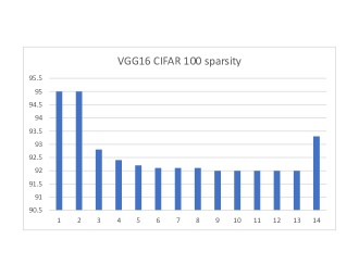
Figure 3: VGG16 on CIFAR100

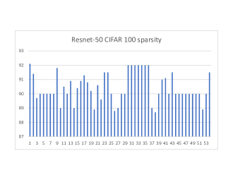
Figure 4: Resnet50 on CIFAR100

All of the presented calculations were performed on the Nvidia Tesla V100-SXM2-32GB. The batch size is always equal 128 (for others or 64 or 256, the proportions are the same) and the final execution time is calculated as the average of 10 iterations. In our experiments, we let the cuDnn library choose the algorithm which would be used to perform convolution for different layers and data types. The tables below, presents the algorithm which was used by the cuDnn library in addition to the execution time for each layer. For each experimental calculation of convolution the $subBatchSize$ was determined (see Section 8) which for last three layers from VGG-16, for $1\times 1$ convolution layers from ResNet50 is 8. For the remaining VGG-16 and some layers and two and for CNN-non static with filter size two, this value is 4, and for CNN-non static with filter size three, this parameter is 2. For DenseNet model this value depend on layer is 4 or 8 (see table 10). The presented results were measured with the optimal value of this parameter. Without setting this value by the method proposed in this paper, it would not be possible to achieve better performance than cuDnn because when the number of block is equal to $numberOfOutputChannel*batchSize$, for VGG-16 and $1x1$ layers, the performance decreased by around $\sim 10\%$. In the case of CNN-non static, the decrease was $\sim 12\%$. An even larger drop in performance occurred when all the data from the batch was processed by $K$ blocks this value was between $\sim 38\%$ and $\sim 45\%$. Table 9 includes the results of time execution for the VGG-16 model model, where for each layers the sparsity was set at $\sim 90\%$ because this is the lowest sparsity level for which the direct sparse convolution algorithm is more effective than the cuDnn library. Despite such a high sparse level, the improvement over the cuDnn was not achieved for every layer. Only for the first and last three layers where the input size in NCHW format, is $3\times 226\times 226$ and $512\times 16\times 16$ respectively, was the improvement gained for float ($\sim 13\%$-first layer and $\sim 12\%$-last layer) and half ($\sim 22\%$-first layer and $\sim 11\%$) data type. In addition, in both cases the algorithm is faster for the half type which is not obvious for the cuDnn library, where for half-precision, the cuDnn always performs convolution by the GEMM algorithm. This way of calculating the convolution on half type, for the VGG-16’s convolution layers with input sizes $64\times 226\times 226$, $256\times 58\times 58$ and $512\times 30\times 30$ is less effective than performing this on float type with the use of FFT or WINOGRAD algorithm. Taking into account only the data in half type format, the sparse approach can additionally improve performance of the VGG-16’s conv layers with the follow input size: $64\times 114\times 114$, $128\times 58\times 58$, $256\times 30\times 30$, $512\times 30\times 30$. Having the same level of sparsity as in the VGG-16 architecture, there is the possibility to achieve better performance than the cuDnn for the $1\times 1$ convolution in Resnet architecture. For this type of convolution, the cuDnn always uses the GEMM algorithm and the result for this are included in Tables 11 and 12. Table 10 contains time result for the same type of convoltuion from DenseNet architecture. In this case the sparsity level and subBatchSize were determined to achieve the best performance for particular layer. The most effective performance of the direct sparse convolution method is achieved for the 1D convolution which is dedicated to the time series data. A significant acceleration compared to cuDnn was reached for the CNN-non static, where for convolution layer with kernel size 2, the sufficient sparsity level is $\sim 77\%$ to gain a $\sim 9\%$ and $\sim 11\%$ speed increase for the float and half data types, respectively (see Tables 13 and 14). In tab.15 real times of pruned VGG-16 (1) are described. The speedup from few to several percent to cuDnn can be observed (see tab.9).

Convolution size (CHWK)	Sparsity [%]	Escoin time - float	Escoin time - half
64x224x224x64	90	60.73	27.08
64x112x112x128	92	15.97	8.64
128x112x112x128	93	27,12	16.22
128x56x56x256	92	12.28	8.42
256x56x56x256	90.8	21.81	14.23
256x28x28x512	92	9.11	5.92
512x28x28x512	92	15.28	13.67
512x14x14x512	92	4.23	4.08

Table 15: Escoin time [ms] for VGG-16 with real sparsity

10 Conclusions and future work

This work is focused on speeding up the convolution operation on GPGPU through the use of the sparse matrix operation and the representation of data at a reduced level of precision. In particular, this strategy makes maximum use of knowledge about the number of produced zero values as a result of the pruning process. The time results obtained from the proposed solution are comparable with the convolution kernel from the cuDnn library, which is recognized as the most effective way to perform convolution on GPGPUs. We have presented concrete cases when it is worth performing convolution using the direct sparse convolution in the cuDnn place. The most improvements are archived for 1D convolution because for this type, the cuDnn library always chooses the GEMM method to perform convolution which does not provide such a strong performance such as the WINOGRAD or the FFT-TILIING method which are used to performing 2D convolution. It is shown that 2D convolution using direct sparse convolution can also outperform cuDnn algorithms. Additionally, we have examined the influence conducting the calculation using reduced precision on time efficiency. The next contribution is showing speedup of DL models on real examples using pruning. It is worth to mention that pruning can significantly improve the accuracy of DL big models when they are used on less complex and reduced datasets. The future works will concentrate on different models on CIFAR100, pruning models based on transfer learning and models for object detection and image segmentation. The pruning will be explored more to check if it is possible to further increase the sparsity. The next approach will adaptation of pruned models in FPGA.

References

- [1] Alex Krizhevsky, Ilya Sutskever, and Geoffrey Hinton. Imagenet classification with deep convolutional neural networks. Neural Information Processing Systems, 25, 01 2012.
- [2] H. Lee and H. Kwon. Going deeper with contextual cnn for hyperspectral image classification. IEEE Transactions on Image Processing, 26(10):4843–4855, 2017.
- [3] Shaoqing Ren, Kaiming He, Ross Girshick, and Jian Sun. Faster r-cnn: Towards real-time object detection with region proposal networks. IEEE Transactions on Pattern Analysis and Machine Intelligence, 39, 06 2015.
- [4] Yoon Kim. Convolutional neural networks for sentence classification. In Proceedings of the 2014 Conference on Empirical Methods in Natural Language Processing (EMNLP), pages 1746–1751, Doha, Qatar, October 2014. Association for Computational Linguistics.
- [5] Krzysztof Wróbel, Michał Karwatowski, Maciej Wielgosz, Marcin Pietroń, and Kazimierz Wiatr. Compression of convolutional neural network for natural language processing. Computer Science, 21(1), 2020.
- [6] Wenpeng Yin, Katharina Kann, Mo Yu, and Hinrich Schütze. Comparative study of cnn and rnn for natural language processing. 02 2017.
- [7] Karel Adámek, Sofia Dimoudi, Mike Giles, and Wes Armour. Gpu fast convolution via the overlap-and-save method in shared memory, 10 2019.
- [8] A. Lavin and S. Gray. Fast algorithms for convolutional neural networks. In 2016 IEEE Conference on Computer Vision and Pattern Recognition (CVPR), pages 4013–4021, 2016.
- [9] Sharan Chetlur, Cliff Woolley, Philippe Vandermersch, Jonathan Cohen, John Tran, Bryan Catanzaro, and Evan Shelhamer. cudnn: Efficient primitives for deep learning, 2014.
- [10] Jack J. Dongarra, Sven Hammarling, Nicholas J. Higham, Samuel D. Relton, Pedro Valero-Lara, and Mawussi Zounon. The design and performance of batched blas on modern high-performance computing systems. In ICCS, 2017.
- [11] Xuhao Chen. Escoin: Efficient sparse convolutional neural network inference on gpus. 2018.
- [12] M. Jordà, P. Valero-Lara, and A. J. Peña. Performance evaluation of cudnn convolution algorithms on nvidia volta gpus. IEEE Access, 7:70461–70473, 2019.
- [13] Baoyuan Liu, Min Wang, Hassan Foroosh, Marshall Tappen, and Marianna Pensky. Sparse convolutional neural networks. pages 806–814, 06 2015.
- [14] L. Lu and Y. Liang. Spwa: An efficient sparse winograd convolutional neural networks accelerator on fpgas. In 2018 55th ACM/ESDA/IEEE Design Automation Conference (DAC), pages 1–6, 2018.
- [15] Alex Krizhevsky, Ilya Sutskever, and Geoffrey E. Hinton. Imagenet classification with deep convolutional neural networks. Commun. ACM, 60(6):84–90, May 2017.
- [16] C. Szegedy, Wei Liu, Yangqing Jia, P. Sermanet, S. Reed, D. Anguelov, D. Erhan, V. Vanhoucke, and A. Rabinovich. Going deeper with convolutions. In 2015 IEEE Conference on Computer Vision and Pattern Recognition (CVPR), pages 1–9, 2015.
- [17] K. He, X. Zhang, S. Ren, and J. Sun. Deep residual learning for image recognition. In 2016 IEEE Conference on Computer Vision and Pattern Recognition (CVPR), pages 770–778, 2016.
- [18] Feiwen Zhu, Jeff Pool, Michael Andersch, Jeremy Appleyard, and Fung Xie. Sparse persistent rnns: Squeezing large recurrent networks on-chip, 2018.
- [19] Marcin Pietron and Maciej Wielgosz. Retrain or not retrain? – efficient pruning methods of deep cnn networks, 2020.
- [20] M. Carbin J. Frankle G.K. Dziugaite, D.M. Roy. The lottery ticket hypothesis at scale, March 2019.
- [21] Alexander M. Rush Victor Sanh, Thomas Wolf. Movement pruning: Adaptive sparsity by fine-tuning, May 2020.
- [22] M. Al-Hami, M. Pietron, R. Casas, and M. Wielgosz. Methodologies of compressing a stable performance convolutional neural networks in image classification, January 2020.
- [23] Song Han, Xingyu Liu, Huizi Mao, Jing Pu, Ardavan Pedram, Mark A. Horowitz, and William J. Dally. Eie: Efficient inference engine on compressed deep neural network. SIGARCH Comput. Archit. News, 44(3):243–254, June 2016.
- [24] Song Han, Jeff Pool, John Tran, and William Dally. Learning both weights and connections for efficient neural network. In Advances in neural information processing systems, pages 1135–1143, 2015.
- [25] D. Lin, S. Talathi, and V. Annapureddy. Fixed point quantization of deep convolutional networks. ICLR, 48:2849–2858, 2016.
- [26] Philipp Gysel. Ristretto: Hardware-oriented approximation of convolutional neural networks. arXiv preprint arXiv:1605.06402, 2016.
- [27] Pietron M. Karwatowski M. Wielgosz M. Duda J. Fast compression and optimization of deep learning models for natural language processing. In CANDAR Workshops 2019, pages 162–168, 2019.
- [28] Prajit Ramachandran, Barret Zoph, and Quoc V. Le. Searching for activation functions. CoRR, abs/1710.05941, 2017.
- [29] Karen Simonyan and Andrew Zisserman. Very deep convolutional networks for large-scale image recognition. arXiv 1409.1556, 09 2014.
- [30] Gao Huang, Zhuang Liu, and Kilian Q. Weinberger. Densely connected convolutional networks. CoRR, abs/1608.06993, 2016.
- [31] S. Winograd. Arithmetic Complexity of Computations. CBMS-NSF Regional Conference Series in Applied Mathematics. Society for Industrial and Applied Mathematics, 1980.
- [32] Jongsoo Park., Sheng Li, Wei Wen, Ping Tak Peter Tang, Hai Li, Yiran Chen, and Pradeep Dubey. Faster cnns with direct sparse convolutions and guided pruning, 2016.
- [33] https://paperswithcode.com/sota/image-classification-on-cifar-100, 2020.
- [34] Song Han, Xingyu Liu, Huizi Mao, Jing Pu, Ardavan Pedram, Mark A. Horowitz, and William J. Dally. Eie: Efficient inference engine on compressed deep neural network. In Proceedings of the 43rd International Symposium on Computer Architecture, ISCA ’16, page 243–254. IEEE Press, 2016.
- [35] Jeffrey Pennington, Richard Socher, and Christopher D Manning. Glove: Global vectors for word representation. In EMNLP, volume 14, pages 1532–1543, 2014.
- [36] Nathan Bell and Michael Garland. Efficient sparse matrix-vector multiplication on CUDA. NVIDIA Technical Report NVR-2008-004, NVIDIA Corporation, December 2008.
- [37] Mingxing Tan and Quoc Le. EfficientNet: Rethinking model scaling for convolutional neural networks. In Kamalika Chaudhuri and Ruslan Salakhutdinov, editors, Proceedings of the 36th International Conference on Machine Learning, volume 97 of Proceedings of Machine Learning Research, pages 6105–6114. PMLR, 09–15 Jun 2019.