Real-Time Intermediate Flow Estimation for Video Frame Interpolation

Abstract

Real-time video frame interpolation (VFI) is very useful in video processing, media players, and display devices. We propose RIFE, a Real-time Intermediate Flow Estimation algorithm for VFI. To realize a high-quality flow-based VFI method, RIFE uses a neural network named IFNet that can estimate the intermediate flows end-to-end with much faster speed. A privileged distillation scheme is designed for stable IFNet training and improve the overall performance. RIFE does not rely on pre-trained optical flow models and can support arbitrary-timestep frame interpolation with the temporal encoding input. Experiments demonstrate that RIFE achieves state-of-the-art performance on several public benchmarks. Compared with the popular SuperSlomo and DAIN methods, RIFE is 4–27 times faster and produces better results. Furthermore, RIFE can be extended to wider applications thanks to temporal encoding.

1 Introduction

Video Frame Interpolation (VFI) aims to synthesize intermediate frames between two consecutive video frames. VFI supports various applications like slow-motion generation, video compression [57], and video frame predition [58]. Moreover, real-time VFI methods running on high-resolution videos have many potential applications, such as reducing bandwidth requirements for live video streaming, providing video editing services for users with limited computing resources, and video frame rate adaption on display devices.

VFI is challenging due to the complex, non-linear motions and illumination changes in real-world videos. Recently, flow-based VFI algorithms have offered a framework to address these challenges and achieved impressive results [30, 22, 40, 62, 3, 61, 28]. Common approaches for these methods involve two steps: 1) warping the input frames according to approximated optical flows and 2) fusing the warped frames using Convolutional Neural Networks (CNNs).

Optical flow models can not be directly used in VFI. Given the input frames $I_{0},I_{1}$, flow-based methods [30, 22, 3] need to approximate the intermediate flows $F_{t\rightarrow 0},F_{t\rightarrow 1}$ from the perspective of the frame $I_{t}$ that we are expected to synthesize. There is a “chicken-and-egg” problem between intermediate flows and frames because $I_{t}$ is not available beforehand, and its estimation is a difficult problem [22, 44]. Many practices [22, 3, 61, 28] first compute bi-directional flows from optical flow models, then reverse and refine them to generate intermediate flows. However, such flows may have flaws in motion boundaries, as the object position changes from frame to frame (“object shift” problem). Appearance Flow [66], A pioneering work in view synthesis, proposes to estimate flow starting from the target view using CNNs. DVF [30] extend it to the voxel flow of dynamic scenes to jointly model the intermediate flow and blend mask to estimate them end-to-end. AdaCoF [27] further extends intermediate flows to adaptive collaborative flows. BMBC [44] designs a bilateral cost volume operator for obtaining more accurate intermediate flows (bilateral motion). In this paper, we aim to build a lightweight pipeline that achieves state-of-the-art (SOTA) performance while maintaining the conciseness of direct intermediate flow estimation. Our pipeline has these main design concepts:

1. Not requiring additional components, like image depth model [3], flow refinement model [22] and flow reversal layer [61], which are introduced to compensate for the defects of intermediate flow estimation. We also want to eliminate reliance on pre-trained SOTA optical flow models that are not tailored for VFI tasks.

2. End-to-end learnable motion estimation: we demonstrate experimentally that instead of introducing some inaccurate motion modeling, it is better to make the CNN learn the intermediate flow end-to-end. This methodology has been proposed [30]. However, the follow-up works do not fully inherit this idea.

3. Providing direct supervision for the approximated intermediate flows: most VFI models are trained with only the final reconstruction loss. Intuitively, propagating gradients of pixel-wise loss across warping operator is not efficient for flow estimation [11, 37, 35]. Lacking supervision explicitly designed for flow estimation degrades the performance of VFI models.

We propose IFNet, which directly estimates intermediate flow from adjacent frames and a temporal encoding input. IFNet adopts a coarse-to-fine strategy [20] with progressively increasing resolution: it iteratively updates the intermediate flows and soft fusion mask via successive IFBlocks. Intuitively, according to the iteratively updated flow fields, we could move corresponding pixels from two input frames to the same location in a latent intermediate frame and use a fusion mask to combine pixels from two input frames. To make our model efficient, unlike most previous optical flow models [15, 20, 54, 19, 56], IFBlocks do not contain expensive operators like cost volume and only use $3\times 3$ convolution and deconvolution as building blocks, which are suitable for resource-constrained devices. Furthermore, plain Conv is highly supported by NPU embedded in display devices and provides convenience for customized requirements. Thanks related researchers for the exploration of efficient models [48, 36, 14].

Employing intermediate supervision is very important. When training the IFNet end-to-end using the final reconstruction loss, our method produces worse results than SOTA methods because of the inaccurate optical flow estimation. The situation dramatically changes after we design a privileged distillation scheme that employs a teacher model with access to the intermediate frames to guide the student to learn.

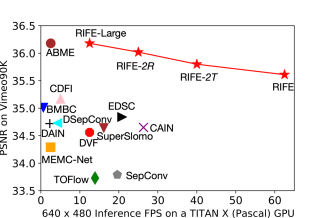
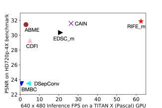
Figure 1: Performance comparison. Results are reported for Vimeo90K [62] and HD-$4\times$ [3] benchmark. More details are in the experimental section

Combining these designs, we propose the Real-time Intermediate Flow Estimation (RIFE). RIFE trained from scratch can achieve satisfactory results, without requiring pre-trained models or datasets with optical flow labels. We illustrate the RIFE’s performance compared with other methods in Figure 1.

To sum up, our main contributions include:

• We design an effective IFNet to approximate the intermediate flows and introduce a privileged distillation scheme to improve the performance.

• Our experiments demonstrate that RIFE achieves SOTA performance on several public benchmarks, especially in the scene of arbitrary-time frame interpolation.

• We show RIFE can be extended to applications such as depth map interpolation and dynamic scene stitching, thanks to its flexible temporal encoding.

2 Related Works

Optical Flow Estimation. Optical flow estimation is a long-standing vision task that aims to estimate the per-pixel motion, useful in many downstream tasks [55, 65, 33, 64]. Since the milestone work of FlowNet [15], flow model architectures have evolved for several years, yielding more accurate results while being more efficient, such as FlowNet2.0 [20], PWC-Net [54] and LiteFlowNet [19]. Recently Teed et al. [56] introduce RAFT, which iteratively updates a flow field through a recurrent unit and achieves a remarkable breakthrough in this field. Another important research direction is unsupervised optical flow estimation [37, 23, 35] which tackles the difficulty of labeling.

Video Frame Interpolation. Recently, optical flow has been a prevalent component in video interpolation. In addition to the method of directly estimating the intermediate flow [30, 27, 44], Jiang et al. [22] propose SuperSlomo using the linear combination of the two bi-directional flows as an initial approximation of the intermediate flows and then refining them using U-Net. Reda et al. [50] and Liu et al. [29] propose to improve intermediate frames using cycle consistency. Bao et al. [3] propose DAIN to estimate the intermediate flow as a weighted combination of bidirectional flow. Niklaus et al. [41] propose SoftSplat to forward-warp frames and their feature map using softmax splatting. Xu et al. [61] propose QVI to exploit four consecutive frames and flow reversal filter to get the intermediate flows. Liu et al. [28] further extend QVI with rectified quadratic flow prediction to EQVI.

Along with flow-based methods, flow-free methods have also achieved remarkable progress. Meyer et al. [38] utilize phase information to learn the motion relationship for multiple video frame interpolation. Niklaus et al. [43] formulate VFI as a spatially adaptive convolution whose convolution kernel is generated using a CNN given the input frames. Cheng et al. propose DSepConv [8] to extend kernel-based method using deformable separable convolution and. Choi et al. [10] propose an efficient flow-free method named CAIN, which employs the PixelShuffle operator and channel attention to capture the motion information implicitly. Some work further focus on increasing the resolution and frame rate of the video together and has achieved good visual effect [59, 60]. In addition, large-motion and animation frame interpolation is also fields of great interest [49, 52, 6].

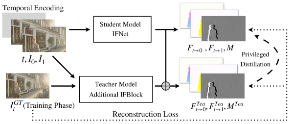
Figure 2: Overview of RIFE pipeline. Given two input frames $I_{0},I_{1}$ and temporal encoding $t$ (timestep encoded as an separate channel [39, 18]), we directly feed them into the IFNet to approximate intermediate flows $F_{t\rightarrow 0},F_{t\rightarrow 1}$ and the fusion map $M$. During the training phase, a privileged teacher refines student’s results based on ground truth $I_{t}$ using a special IFBlock

Knowledge Distillation. Our privileged distillation [31] for intermediate flow conceptually belongs to the knowledge distillation [17], which originally aims to transfer knowledge from a large model to a smaller one. In privileged distillation, the teacher model gets more input than the student model, such as scene depth, images from other views, and even image annotation. Therefore, the teacher model can provide more accurate representations to guide the student model to learn. This idea is applied to some computer vision tasks, such as hand pose estimation [63], re-identification [46] and video style transfer [7]. Our work is also related to codistillation [1] where the student and teacher have the same architecture and different inputs during training.

3 Method

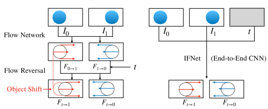
Figure 3: Compare indirect intermediate flow estimation [22, 61, 3] (left) with IFNet (right). As the object shifts, flow reversal modules may have flaws in motion boundaries. Rather than hand-engineering flow reversal layers, CNNs can learn intermediate flow estimates end-to-end

3.1 Pipeline Overview

We illustrate the overall pipeline of RIFE in Figure 2. Given a pair of consecutive RGB frames, $I_{0},I_{1}$ and target timestep $t~{}(0\leq t\leq 1)$, our goal is to synthesize an intermediate frame $\widehat{I}_{t}$. We estimate the intermediate flows $F_{t\rightarrow 0}$, $F_{t\rightarrow 1}$ and fusion map $M$ by feeding input frames and $t$ as an additional channel into the IFNet. We can get reconstructed image $\widehat{I}_{t}$ using following formulation:

$$\widehat{I}_{t}=M\odot\widehat{I}_{t\leftarrow 0}+(1-M)\odot\widehat{I}_{t\leftarrow 1},$$ (1)

$$\widehat{I}_{t\leftarrow 0}=\overleftarrow{\mathcal{W}}(I_{0},F_{t\rightarrow 0}),\quad\widehat{I}_{t\leftarrow 1}=\overleftarrow{\mathcal{W}}(I_{1},F_{t\rightarrow 1}).$$ (2)

where $\overleftarrow{\mathcal{W}}$ is the image backward warping, $\odot$ is an element-wise multiplier, and M is the fusion map $(0\leq M\leq 1)$. We use another encoder-decoder CNNs named RefineNet following previous methods [22, 41] to refine the high-frequency area of $\widehat{I}_{t}$ and reduce artifacts of the student model. Its computational cost is similar to the IFNet. The RefineNet finally produce a reconstruction residual $\Delta~{}(-1\leq\Delta\leq 1)$. And we will get a refined reconstructed image $\widehat{I}_{t}+\Delta$. The detailed architecture of RefineNet is in the Appendix.

3.2 Intermediate Flow Estimation

Some previous VFI methods reverse and refine bi-directional flows [22, 61, 3, 28] as depicted in Figure 3. The flow reversal process is usually cumbersome due to the difficulty of handling the changes of object positions. Intuitively, the previous flow reversal method hopes to perform spatial interpolation on the optical flow field, which is not trivial because of the “object shift” problem. The role of our IFNet is to directly and efficiently predict $F_{t\rightarrow 0},F_{t\rightarrow 1}$ and fusion mask $M$ given two consecutive input frames $I_{0},I_{1}$ and timestep $t$. When $t=0$ or $t=1$, IFNet is similar to the classical optical flow models.

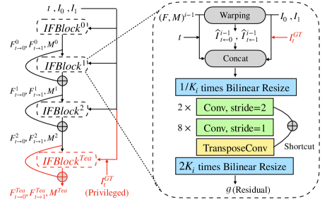
Figure 4: Left: The IFNet is composed of several stacked IFBlocks operating at different resolution. Right: In an IFBlock, we first backward warp the two input frames based on current approximated flow $F^{i-1}$. Then the input frames $I_{0},I_{1}$, warped frames $\widehat{I}_{t\leftarrow 0},\widehat{I}_{t\leftarrow 1}$, the previous results $F^{i-1},M^{i-1}$ and timestep $t$ are fed into the next IFBlock to approximate the residual of flow and mask. The privileged information $I_{t}^{GT}$ is only provided for teacher

To handle the large motion encountered in intermediate flow estimation, we employ a coarse-to-fine strategy with gradually increasing resolution, as illustrated in Figure 4. Specifically, we first compute a rough prediction of the flow on low resolution, which is believed to capture large motions easier, then iteratively refine the flow fields with gradually increasing resolution. Following this design, our IFNet has a stacked hourglass structure, where a flow field is iteratively refined via successive IFBlocks:

$$\left[\begin{array}[]{c}F^{i}\\ M^{i}\end{array}\right]=\left[\begin{array}[]{c}F^{i-1}\\ M^{i-1}\end{array}\right]+\text{IFB}^{i}(\left[\begin{array}[]{c}F^{i-1}\\ M^{i-1}\end{array}\right],t,\widehat{I}^{i-1}),$$ (3)

where $F^{i-1}$ and $M^{i-1}$ denote the current estimation of the intermediate flows and fusion map from the $(i-1)^{th}$ IFBlock, and $\text{IFB}^{i}$ represents the $i^{th}$ IFBlock. We use a total of 3 IFBlocks, and each has a resolution parameter, $(K^{0},K^{1},K^{2})=(4,2,1)$. During inference time, the final estimation is $F^{n}$ and $M^{n}(n=2)$. Each IFBlock has a feed-forward structure consisting of serveral convolutional layers and an up-sampling operator. Except for the layer that outputs the optical flow residuals and the fusion map, we use PReLU [16] as the activation function. The cost volume [15] operator is computationally expensive and usually ties the starting point of optical flow to the input image. So it is not directly transferable.

Table 1: Average inference time on the $640\times 480$ frames. Recent VFI methods [22, 3, 41] run the optical flow model twice to obtain bi-directional flows

Method	FlowNet2.0 [20]	PWC-Net [54]	LiteFlownet [19]	RAFT [56]	IFNet
Runtime	$2\times 207$ms	$2\times 21$ms	$2\times 73$ms	$2\times 52$ms	7ms

We compare the runtime of the SOTA optical flow models [54, 19, 56] and IFNet in Table 1. Current flow-based VFI methods [22, 3, 41] usually need to run their flow models twice then process the bi-directional flows. Therefore the intermediate flow estimation in RIFE runs at a faster speed. Although these optical models can estimate inter-frame motion accurately, they are not suitable for direct migration to VFI tasks.

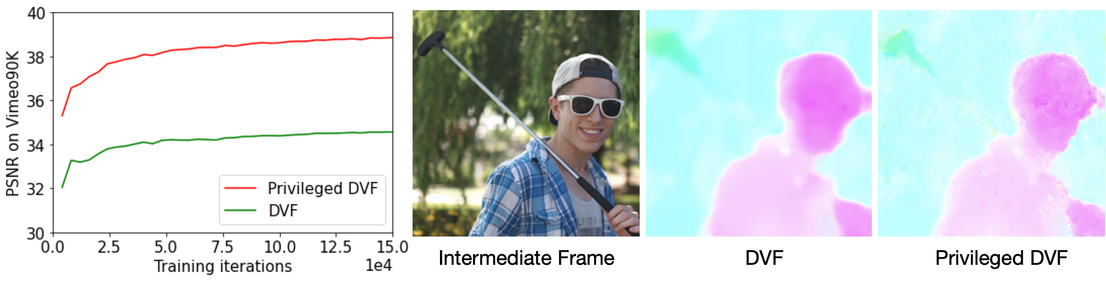
Figure 5: Results of DVF [30] (Vimeo90K). After feeding the edge map of intermediate frames (privileged information) into the model, the estimated flows can be significantly improved, resulting in better reconstruction on validation set

3.3 Priveleged Distillation for Intermediate Flow

We use an experiment to show that directly approximating the intermediate flows is challenging without access to the intermediate frame. We train DVF [30] model to estimate intermediate flow on Vimeo90K [62] dataset. As a comparison, we add an additional input channel to the DVF model, containing the edge map [12] of intermediate frames (denoted as “Privileged DVF”). Figure 5 shows that the quantization result of Privileged DVF is surprisingly high, while the flows estimated by DVF are blurry. Similar conclusions are also demonstrated in deferred rendering, showing that VFI will be simpler with some intermediate information [6]. This demonstrates that estimating optical flow between two images is easier for the model than estimating intermediate flow. This inspire us to design a privileged model to teach the original model.

We design a privileged distillation loss to IFNet. We stack an additional IFBlock (teacher model $\text{IFB}^{Tea}$, $K^{Tea}=1$) that refines the results of IFNet referring to the target frame $I^{GT}_{t}$:

$$\left[\begin{array}[]{c}F^{Tea}\\ M^{Tea}\end{array}\right]=\left[\begin{array}[]{c}F^{n}\\ M^{n}\end{array}\right]+\text{IFB}^{Tea}(\left[\begin{array}[]{c}F^{n}\\ M^{n}\end{array}\right],t,\widehat{I}^{n},I^{GT}_{t}).$$ (4)

With the access of $I^{GT}_{t}$ as privileged information, the teacher model produces more accurate flows. We define the distillation loss $\mathcal{L}_{dis}$ as follows:

$$\mathcal{L}_{dis}=\sum_{i\in\{0,1\}}||F_{t\rightarrow i}-F^{Tea}_{t\rightarrow i}||_{2}.$$ (5)

We apply the distillation loss over the full sequence of predictions generated from the iteratively updating process in the student model. The gradient of this loss will not be backpropagated to the teacher model. The teacher block will be discarded after the training phase, hence this would incur no extra cost for inference. It makes more stable training and faster convergence.

3.4 Implementation Details

Supervisions. Our training loss $\mathcal{L}_{total}$ is a linear combination of the reconstruction losses $\mathcal{L}_{rec},\mathcal{L}^{Tea}_{rec}$ and privileged distillation loss $\mathcal{L}_{dis}$:

$$\mathcal{L}_{total}=\mathcal{L}_{rec}+\mathcal{L}^{Tea}_{rec}+\lambda_{d}\mathcal{L}_{dis},$$ (6)

where we set $\lambda_{d}=0.01$ to balance the scale of losses.

The reconstruction loss $\mathcal{L}_{rec}$ models the reconstruction quality of the intermediate frame. The reconstruction loss has the formulation of:

$$\mathcal{L}_{rec}=d(\widehat{I}_{t},{I}^{GT}_{t}),\mathcal{L}_{rec}^{Tea}=d(\widehat{I}_{t}^{Tea},{I}^{GT}_{t}),$$ (7)

where $d$ is often a pixel-wised loss. Following previous work [40, 41], we use $L_{1}$ loss between two Laplacian pyramid representations of the reconstructed image and ground truth (denoted as $L_{Lap}$, the pyramidal level is $5$).

Training Dataset. We use the Vimeo90K dataset [62] to train RIFE. This dataset has $51,312$ triplets for training, where each triplet contains three consecutive video frames with a resolution of $448\times 256$. We randomly augment the training data using horizontal and vertical flipping, temporal order reversing, and rotating by $90$ degrees.

Training Strategy. We train RIFE on the Vimeo90K training set and fix $t=0.5$. RIFE is optimized by AdamW [32] with weight decay $10^{-4}$ on $224\times 224$ patches. Our training uses a batch size of $64$. We gradually reduce the learning rate from $10^{-4}$ to $10^{-5}$ using cosine annealing during the whole training process. We train RIFE on $8$ TITAN X (Pascal) GPUs for $300$ epochs in $10$ hours.

We use the Vimeo90K-Septuplet [62] dataset to extend RIFE to support arbitrary-timestep frame interpolation [9, 24]. This dataset has $91,701$ sequence with a resolution of $448\times 256$, each of which contains $7$ consecutive frames. For each training sample, we randomly select $3$ frames $(I_{n_{0}},I_{n_{1}},I_{n_{2}})$ and calculate the target timestep $t=(n_{1}-n_{0})/(n_{2}-n_{0})$, where $0\leq n_{0}<n_{1}<n_{2}<7$. So we can write RIFE’s temporal encoding to extend it. We keep other training setting unchanged and denote the model trained on Vimeo90K-Septuplet as RIFE_m.

4 Experiments

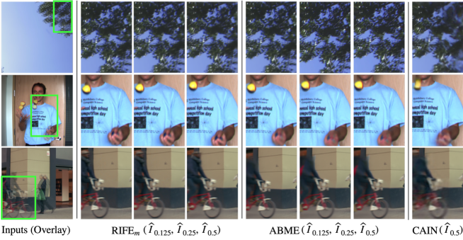
Figure 6: Interpolating multiple frames using RIFE_m. These images are from HD [3], M.B. [2], Vimeo90K [62] benchmarks, respectively. We attach the results of CAIN [10] and ABME [45]. RIFE_m provides smooth and continuous motions

We first introduce the benchmarks for evaluation. Then we provide variants of our models with different computational costs. We compare these models with representative SOTA methods. In addition, we show the capability of generating arbitrary-timestep frames and other applications using RIFE. An ablation study is carried out to analyze our design. Finally, we discuss some limitations of RIFE.

4.1 Benchmarks and Evaluation Metrics

We train our models on the Vimeo90K training dataset and directly test it on the following benchmarks.

Vimeo90K. There are 3,782 triplets in the Vimeo90K testing set [62] with resolution of $448\times 256$. This dataset is widely evaluated in recent VFI methods.

UCF101. The UCF101 dataset [53] contains videos with various human actions. There are 379 triplets with a resolution of $256\times 256$.

HD. Bao et al. [4] collect 11 videos for evaluation. The HD benchmark consists of four 1080p, three 720p and four $1280\times 544$ videos. Following the author of this benchmark, we use the first 100 frames of each video for evaluation.

X4K-1000FPS. A recently released high frame rate 4K dataset [51] containing $15$ scenes for testing. We follow the evaluation of [45, 45].

We measure the peak signal-to-noise ratio (PSNR), structural similarity (SSIM), and interpolation error (IE) for quantitative evaluation. All the methods are tested on a TITAN X (Pascal) GPU. To report the runtime, we test all models for processing a pair of $640\times 480$ images using the same device. Disagreements with some of the published results are explained in the Appendix.

4.2 Comparisons with Previous Methods

We compare RIFE with previous VFI models [62, 43, 4, 3, 10, 41, 44, 8, 27, 13, 9]. These models are officially released except SoftSplat [41]. A recently unofficial reproduction [49] report SoftSplat [41] is slower than ABME [45], and we can not verify it with the available materials. In addition, we train DVF [30] model and SuperSlomo [22] using our training pipeline on Vimeo90K dataset because the released models of these methods are trained on early datasets.

Table 2: Quantitative evaluation (PSNR) for $4\times$ interpolation on the HD [4] and 8$\times$ interpolation on X4K-1000FPS [51] benchmark. The 544p videos of HD benchmark are relatively more dynamic. Thus the PSNR index of these 544p videos is lower

Method	Arbitrary-timestep	HD544p	HD720p	HD1080p	X4K-1000FPS
DAIN [3]	✓	22.17	30.25	OOM	26.78${\dagger}$
CAIN [10]	-	21.81	31.59	31.08	-
BMBC [44]	✓	19.51	23.47	OOM	OOM
DSepconv [8]	-	19.28	23.48	OOM	OOM
CDFI [13]	-	21.85	29.28	OOM	OOM
EDSCm [9]	✓	21.89	30.35	30.91	-
ABME [45]	-	22.46	31.43	33.22	30.16${\dagger}$
RIFEm	✓	22.95	31.87	34.25	30.58${\ddagger}$

• ${\dagger}$: copy from [45]. ${\ddagger}$: estimate flows on 1/4 downsampled videos.

Interpolating Arbitrary-timestep Frame. Arbitrary-timestep VFI is important in frame-rate conversion. We apply RIFE_m to interpolate multiple intermediate frames at different timesteps $t\in(0,1)$, as shown in Figure 6. RIFE_m can successfully handle $t=0.125~{}(8\times)$ which is not included in the training data.

To provide a quantitative comparison of multiple frame interpolation, we further extract every fourth frame of videos from HD benchmark [4] and use them to interpolate other frames. We divide the HD benchmark into three subsets with different resolution to test these methods. We show the quantitative PSNR between generated frames and frames of the original videos in Table 2. Note that DAIN [3], BMBC [44] and EDSC_m [8] can generate a frame at an arbitrary timestep. Some other methods can only interpolate the intermediate frame at $t=0.5$. Thus we use them recursively to produce $4\times$ results. Specifically, we firstly apply the single interpolation method once to get intermediate frame $\widehat{I}_{0.5}$. Then we feed $I_{0}$ and $\widehat{I}_{0.5}$ to get $\widehat{I}_{0.25}$ and so on. Furthermore, we test $8\times$ interpolation in a recently released dataset, X4K-1000FPS [51]. Overall, RIFE_m is very effective in the multiple frame interpolation.

Model Scaling. To scale our models that can be compared with existing methods, we introduce two modifications following: test-time augmentation and resolution multiplying. 1) We flip the input images horizontally and vertically to get augmented test data. We infer and average (with flipping) these two results finally. This model is denoted as RIFE-2T. 2) We remove the first downsample layer of IFNet and add a downsample layer before its output to match the origin pipeline. We also perform this modification on RefineNet. It enlarges the process resolution of the feature maps and produces a model named RIFE-2R. We combine these two modifications to extend RIFE to RIFE-Large (2T2R).

Table 3: Quantitative comparisons on several benchmarks. The images of each dataset are directly inputted to each model. Some models are unable to run on 1080p images due to exceeding the memory available on our graphics card (denoted as “OOM”). We use gray backgrounds to mark the methods that require pre-trained depth models or optical flow models

Method	# Parameters	Runtime	UCF101 [53]		Vimeo90K [62]		M.B. [2]	HD [3]
	(Million)	(ms)	PSNR	SSIM	PSNR	SSIM	IE	PSNR
DVF [62]	1.6	80	34.92	0.968	34.56	0.973	2.47	31.47
TOFlow [2]	1.1	84	34.58	0.967	33.73	0.968	2.15	29.37
DAIN [3]	24.0	436	35.00	0.968	34.71	0.976	2.04	31.64†
DSepConv [8]	21.8	236	35.08	0.969	34.73	0.974	2.03	OOM
SoftSplat [41]†	7.7	-	35.39	0.970	36.10	0.980	1.81	-
BMBC [44]	11.0	1580	35.15	0.969	35.01	0.976	2.04	OOM
CDFI [13]	5.0	198	35.21	0.969	35.17	0.977	1.98	OOM
ABME [45]	18.1	339	35.37	0.970	36.18	0.981	1.88	32.17
RIFE-Large	9.8	80	35.41	0.970	36.19	0.981	1.82	32.31
Relatively Fast Models
CAIN [10]	42.8	38	34.98	0.969	34.65	0.973	2.28	31.77
Superslomo [22]	19.8	62	35.15	0.968	34.64	0.974	2.21	31.55
SepConv [42]	21.6	51	34.78	0.967	33.79	0.970	2.27	30.87
AdaCoF [27]	21.8	34	34.91	0.968	34.27	0.971	2.31	31.43
EDSC [9]	8.9	46	35.13	0.968	34.84	0.975	2.02	31.59
RIFE	9.8	16	35.28	0.969	35.61	0.978	1.96	32.14
RIFE${}_{m}{\ddagger}$	9.8	16	35.22	0.969	35.46	0.978	2.16	32.31

• ${\dagger}$: copy from the original papers. ${\ddagger}$: trained on Vimeo90K-Septuplet dataset.

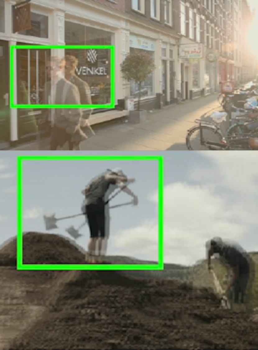
Inputs

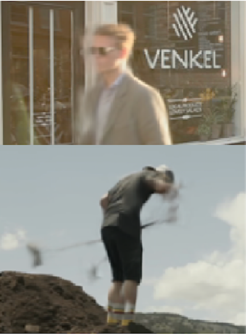
SepConv [42]

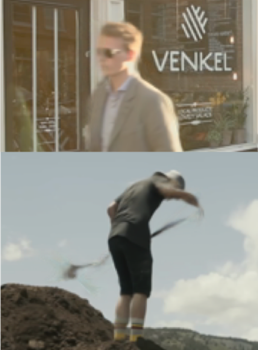
DAIN [3]

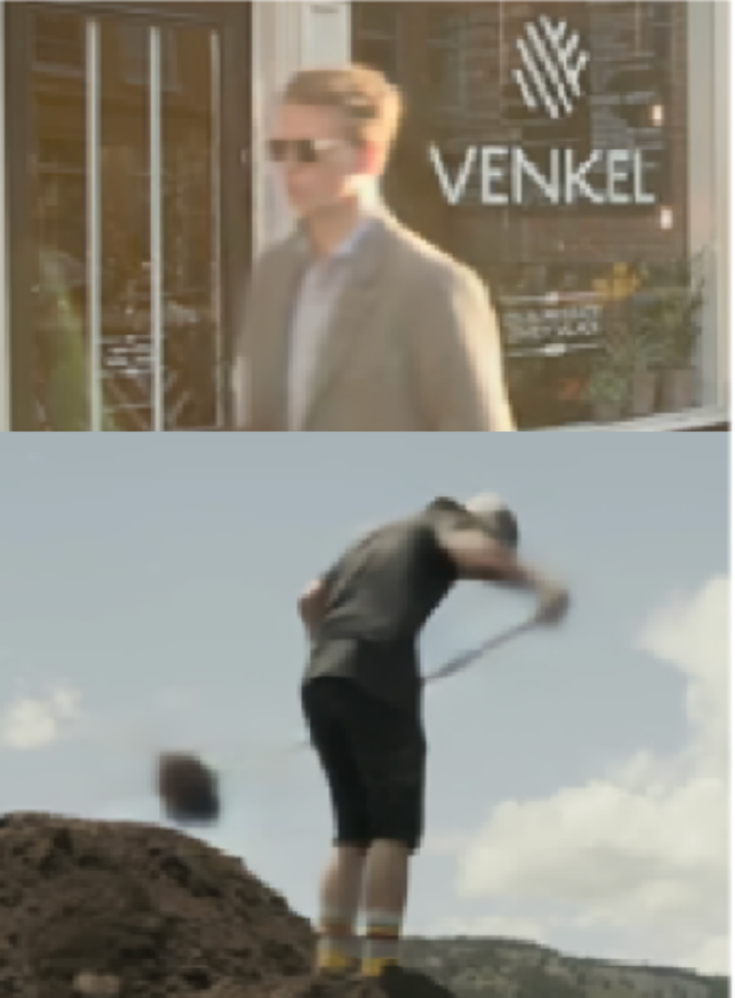
CAIN [10]

RIFE (Ours)

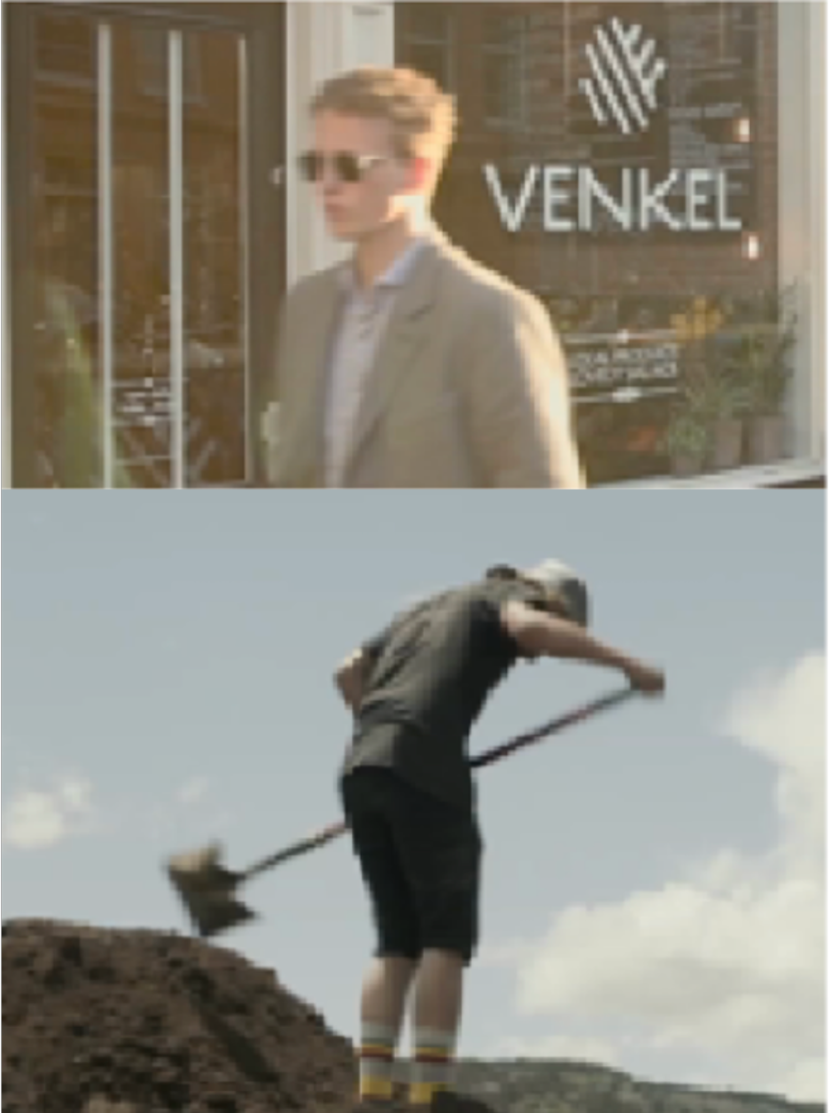
GT

Figure 7: Qualitative comparison on Vimeo90K [62] testing set

Middle Timestep Interpolation. We report the performance of middle timestep interpolation in Table 3. For ease of comparison, we group the models by running speed. RIFE achieve very high performance compared to other small models. Meanwhile, RIFE needs only about $3$ gigabytes of GPU memory to process 1080p videos. We get a larger version of our model (RIFE-Large) by model scaling, which runs about $4\times$ faster than ABME [45] with comparable performance. We provide a visual comparison of video clips with large motions from the Vimeo90K testing set in Figure 7, where SepConv [43] and DAIN [3] produce ghosting artifacts, and CAIN [10] causes missing-parts artifacts. Overall, RIFE (with small computation) can produce more reliable results.

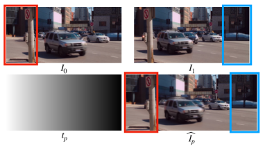
Figure 8: Synthesize images from two views on one “panoramic” image $\widehat{I}_{p}$ using RIFE_m. $\widehat{I}_{p}$ has been stretched for better visualization

4.3 General Temporal Encode

In the VFI task, our temporal encoding $t$ is used to control the timestep. To show its generalization capability, we demonstrate that we can control this encoding to implement diverse applications. As shown in Figure 8, if we input a gradient encoding $t_{p}$, the RIFE_m will synthesize the two images from dynamic scenes in a “panoramic” view  (use different timestamps for each column). The position relation of the vehicle in $\widehat{I}_{p}$ is between $I_{0}$ and $I_{1}$. In other words, if $I_{0}$, $I_{1}$ are from the binocular camera, the shooting time of $I_{1}$ is later than that of $I_{0}$. $\widehat{I}_{p}$ is the result of a wider FOV camera scan in columns. Similarly, this method may potentially eliminate the rolling shutter of the videos by having different timestamps for each horizontal row.

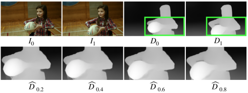
Figure 9: Interpolation for depth map using RIFE_m.

Table 4: Ablation study on distillation scheme, intermediate flow estimation, model design and loss function

Setting	Vimeo90K [62]	MiddleBury [2]	Runtime
	PSNR	IE	$640\times 480$
Intermediate Flow Estimation
RAFT [56] + linear reversal [22]	34.68	2.31	60ms
RAFT [56] + CNN reversal	34.82	2.24	65ms
RAFT [56] + reversal layer [28]	35.16	2.04	101ms
PWC-Net [54] + reversal layer [28]	35.24	2.06	83ms
PWC-Net [54] + forward warping [41]	35.48	2.02	52ms
RIFE	35.61	1.96	16ms
Distillation Scheme
RIFE w/ self-consistency	35.37	2.02	16ms
RIFE w/ RAFT-KD	35.52	1.98	16ms
RIFE (priviledged distillation)	35.61	1.96	16ms
Model Design
RIFE w/ one IFBlock	35.17	2.12	12ms
RIFE w/ two IFBlocks	35.46	1.97	14ms
RIFE + BN [21]	35.49	2.02	21ms
RIFE	35.61	1.96	16ms
Loss Function
RIFE w/ $L_{1}$	35.51	1.94	16ms
RIFE w/ $L_{Lap}$	35.61	1.96	16ms

4.4 Image Representation Interpolation

RIFE_m can interpolate other image representations using the intermediate flows and fusion map approximating from images. For instance, we interpolate the results of MiDaS [47] which is a popular monocular depth model, shown in Figure 9. The synthesis formula is simply as follows:

$$\widehat{D}_{t}=M\odot\overleftarrow{\mathcal{W}}(D_{0},F_{t\rightarrow 0})+(1-M)\odot\overleftarrow{\mathcal{W}}(D_{1},F_{t\rightarrow 1}),$$ (8)

where $D_{0},D_{1}$ are estimated by MiDas [47] and $F,M$ are estimated by RIFE_m. RIFE may potentially be used to extend some models and provide visually plausible effects when we ignore z-axis motion of objects.

4.5 Ablation Studies

We design some ablation studies on the intermediate flow estimation, distillation scheme, model design and loss function, shown in Table 4. These experiments use the same hyper-parameter setting and evaluation on Vimeo90K [62] and MiddleBury [2] benchmarks.

IFNet vs. Flow Reversal. We compare IFNet with previous intermediate flow estimation methods. Specifically, we use RAFT [56] and PWC-Net [54] with officially pre-trained parameters to estimate the bi-directional flows. Then we implement three flow reversal methods, including linear reversal [22], using a hidden convolutional layer with $128$ channels, and the flow reversal layer from EQVI [28]. The optical flow models and flow reversal modules are combined together to replace the IFNet. Furthermore, we try to use the forward warping [41] operator to bypass flow reversal. These models are jointly fine-tuned with RefineNet. Because these models can not directly approximate the fusion map, the fusion map is subsequently approximated by RefineNet. As shown in Table 4, RIFE is more efficient and gets better interpolation performance. These flow models can estimate accurate bi-directional optical flow, but the flow reversal has difficulties in dealing with the object shift problem illustrated in Figure 3.

Ablation on the Distillation Scheme. We observe that removing the distillation framework makes model training sometimes divergent. Furthermore, we show the importance of distillation design in following experiments. a1) Remove the privileged teacher block and use the last IFBlock’s results to guide the first two IFBlocks, denoted as “self-consistency”; a2) Use pre-trained RAFT [56] to estimate the intermediate flows based on the ground truth image, denoted as “RAFT-KD”. This guidance is inspired by the pseudo-labels method [26]. However, this implementation relies on the pre-trained optical flow model and extremely increases the training duration ($3\times$). We found a1 and a2 suffer in quality. These experiments demonstrate the importance of optical flow supervision. Some recent work [25, 34] has also echoed the improvement using suitable optical flow distillation.

Ablation on RIFE’s Architecture and Loss Function. To verify the coarse-to-fine strategy of IFNet, we removed the first IFBlock and the first two IFBlocks in two experiments, respectively. We also try some other popular techniques, such as Batch Normlization (BN) [21]. BN does stabilize the training, but degrades final performance and increases inference overhead. We provide a pair of experiments to show $L_{Lap}$ [40, 41] is quantitatively better than $\mathcal{L}_{1}$.

Limitations. Our work may not cover some practical application requirements. Firstly, RIFE focuses on using two input frames and multi-frame input [61, 28, 24] is left to future work. One straightforward approach is to extend IFNet to use more frames as input. Secondly, most experiments are done with SSIM and PSNR as quantitative indexes. If human perception quality is preferred, RIFE can readily be changed to use the perceptually related losses [5, 42]. Thirdly, additional training data may be necessary for extending RIFE to various applications, such as interpolation for depth map and animation videos [52].

5 Conclusion

We develop an efficient and flexible algorithm for VFI, namely RIFE. A separate neural module IFNet directly estimates the intermediate optical flows, supervised by a privileged distillation scheme, where the teacher model can access the ground truth intermediate frames. Experiments confirm RIFE can effectively process videos of different scenes. Furthermore, an extra input with temporal encoding enables RIFE for arbitrary-timestep frame interpolation. The lightweight nature of RIFE makes it much more accessible for downstream tasks.

Acknowledgment

This work is supported by National Key R&D Program of China (2021ZD0109803) and National Natural Science Foundation of China under Grant No. 62136001, 62088102.

6 Appendix

6.1 Architecture of RefineNet

Following the previous work [41], we design a RefineNet with an encoder-decoder architecture similar to U-Net and a context extractor. The context extractor and encoder part have similar architectures, consisting of four convolutional blocks, and each of them is composed of two $3\times 3$ convolutional layers, respectively. The decoder part in the FusionNet has four transpose convolution layers.

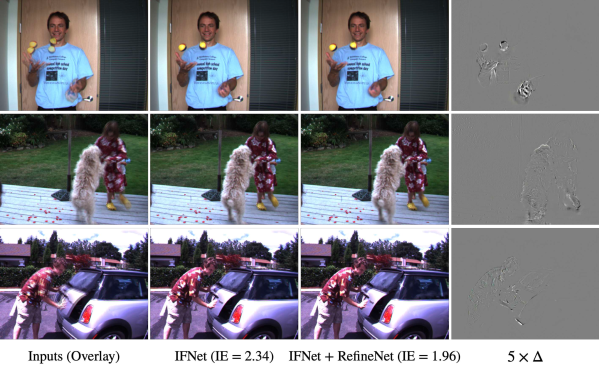
Figure 10: Visualization of the effect of RefineNet on M.B. [2] benchmark.

Specifically, the context extractor first extracts the pyramid contextual features from input frames separately. We denote the pyramid contextual feature as $C_{0}$: $\{C_{0}^{0},C_{0}^{1},C_{0}^{2},C_{0}^{3}\}$ and $C_{1}$: $\{C_{1}^{0},C_{1}^{1},C_{1}^{2},C_{1}^{3}\}$. We then perform backward warping on these features using estimated intermediate flows to produce aligned pyramid features, $C_{t\leftarrow 0}$ and $C_{t\leftarrow 1}$. The origin frames $I_{0},I_{1}$, warped frames $\widehat{I}_{t\leftarrow 0},\widehat{I}_{t\leftarrow 1}$, intermediate flows $F_{t\rightarrow 0},F_{t\rightarrow 1}$ and fusion mask $M$ are fed into the encoder. The output of $i-th$ encoder block is concatenated with the $C_{t\leftarrow 0}^{i}$ and $C_{t\leftarrow 1}^{i}$ before being fed into the next block. The decoder parts finally produce a reconstruction residual $\Delta$. And we will get a refined reconstructed image $clamp(\hat{\mathbf{I}}_{t}+\Delta,0,1)$, where $\hat{\mathbf{I}}_{t}$ is the reconstruct image before the RefineNet. We show some visualization results in Figure 10. RefineNet seems to make some uncertain areas more blurred to improve quantitative results.

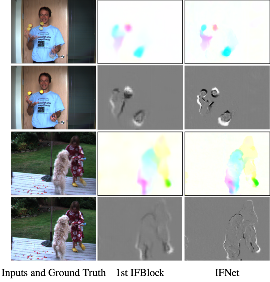
Figure 11: Visualization of intermediate flow $F_{t\rightarrow 0}$ and blend mask $M$. We show that stack 3 IFblocks can get finer intermediate flow and blend mask.

6.2 Selection of Building Operators

We focus on introducing a simplified VFI pipeline without bells and whistles. So we choose building operators with intentional restraint. Exploring model compression is orthogonal to our approach. Our pipeline can be further sped up by manual model design, or Neural Architecture Search (NAS) approaches (left to future work). Furthermore, plain Conv is highly supported by NPU embedded in display devices and provides convenience for customized requirements.

6.3 Intermediate Flow Visualization

In Figure 12, we provide visual results of our IFNet and compare them with the linearly combined bi-directional optical flows [22]. IFNet produces clear motion boundaries.

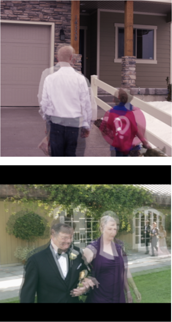
Inputs (Overlay)

Combination

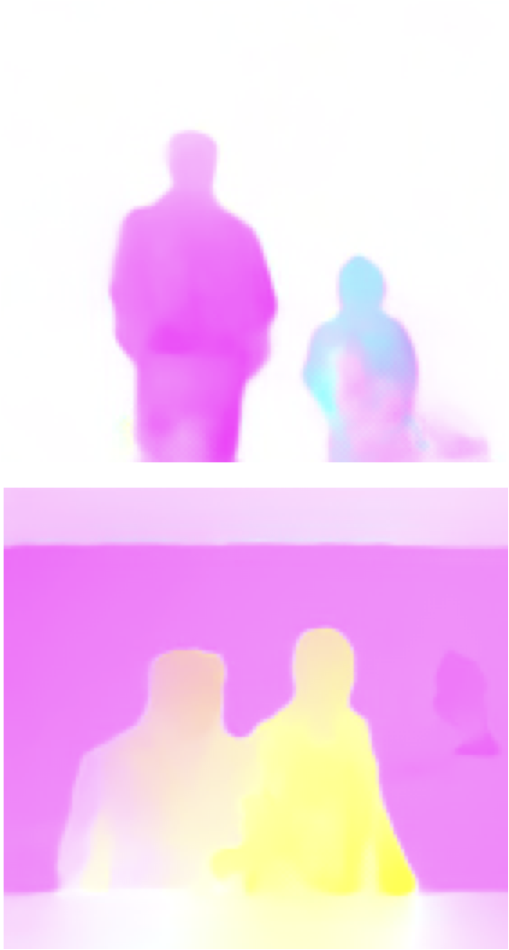
IFNet

Figure 12: Visual comparison between linearly combined bi-directional flows [22] and the result of IFNet.

6.4 Model Efficiency Comparison

Recall that we aim to explore real-time models instead of refreshing SOTA with larger models. Our models are suitable for real-time processing scenarios (display devices, live streaming, games) and media post-processing. However, to the best of our knowledge, currently published papers do not test the speed of each state-of-the-art VFI model on same hardware, and rarely report the complexity of the model. Some previous works [3, 45] report runtime data from the MiddleBury public leaderboard without indicating running devices. These data are reported by the submitters of various methods. A more verifiable survey comes from EDSC (Table 10) [9]. We collect the models of each paper and test them on a NVIDIA TITAN X(Pascal) GPU with same hardware. The code can be found on https://github.com/megvii-research/ECCV2022-RIFE/blob/main/benchmark/testtime.py. RIFE use $16ms$ for interpolating a $640\times 480$ frame, $31ms$ for 720p frame, $68ms$ for 1080p frame. The relationship between runtime and resolution is roughly linear.

Take into account the imprecise comparison issues that TTA may introduce. We can use other techniques to get large models. We replace TTA with “multiply the number of hidden filter’s channel by a factor of $1.5$”. And we train this new large model from scratch. The difference between its performance and RIFE-Large is almost negligible. $2\times$ TTA do not change the performance curve of our model. Using TTA, we can get a larger model without training.

6.5 Other Details

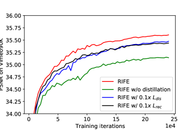
Figure 13: PSNR on Vimeo90K benchmark during the whole training process. The distillation scheme helps RIFE converge to better performance

Training dynamic. We study the dynamic during the RIFE training. As shown in Figure 13, the privileged distillation scheme helps RIFE converge to better performance. Furthermore, we try to adjust the weights of losses. We found that larger scale$~{}(10\times)$ of weights will cause the model to not converge and smaller weights$~{}(0.1\times)$ will slightly reduce model performance. We found that the effect of our distillation method is similar to regularization techniques, making the models easier to train.

Supervision of mask. Further experiment show that adding supervision of fusion mask has no effect. More detailed distillation design may be a future research direction. When fixing $\widehat{I}_{t\leftarrow 0}$ and $\widehat{I}_{t\leftarrow 1}$, $M$ can be directly learned from the ground truth using the reconstruction loss.

References

- [1] Anil, R., Pereyra, G., Passos, A., Ormandi, R., Dahl, G.E., Hinton, G.E.: Large scale distributed neural network training through online distillation. In: Proceedings of the International Conference on Learning Representations (ICLR) (2018)
- [2] Baker, S., Scharstein, D., Lewis, J., Roth, S., Black, M.J., Szeliski, R.: A database and evaluation methodology for optical flow. In: International Journal of Computer Vision (IJCV) (2011)
- [3] Bao, W., Lai, W.S., Ma, C., Zhang, X., Gao, Z., Yang, M.H.: Depth-aware video frame interpolation. In: Proceedings of the IEEE Conference on Computer Vision and Pattern Recognition (CVPR) (2019)
- [4] Bao, W., Lai, W.S., Zhang, X., Gao, Z., Yang, M.H.: Memc-net: Motion estimation and motion compensation driven neural network for video interpolation and enhancement. IEEE Transactions on Pattern Analysis and Machine Intelligence (IEEE TPAMI) (2018). https://doi.org/10.1109/TPAMI.2019.2941941
- [5] Blau, Y., Michaeli, T.: The perception-distortion tradeoff. In: Proceedings of the IEEE Conference on Computer Vision and Pattern Recognition (CVPR) (2018)
- [6] Briedis, K.M., Djelouah, A., Meyer, M., McGonigal, I., Gross, M., Schroers, C.: Neural frame interpolation for rendered content. ACM Transactions on Graphics (TOG) 40(6), 1–13 (2021)
- [7] Chen, X., Zhang, Y., Wang, Y., Shu, H., Xu, C., Xu, C.: Optical flow distillation: Towards efficient and stable video style transfer. In: Proceedings of the European Conference on Computer Vision (ECCV) (2020)
- [8] Cheng, X., Chen, Z.: Video frame interpolation via deformable separable convolution. In: AAAI Conference on Artificial Intelligence (2020)
- [9] Cheng, X., Chen, Z.: Multiple video frame interpolation via enhanced deformable separable convolution. IEEE Transactions on Pattern Analysis and Machine Intelligence (TPAMI) (2021). https://doi.org/10.1109/TPAMI.2021.3100714
- [10] Choi, M., Kim, H., Han, B., Xu, N., Lee, K.M.: Channel attention is all you need for video frame interpolation. In: AAAI Conference on Artificial Intelligence (2020)
- [11] Danier, D., Zhang, F., Bull, D.: Spatio-temporal multi-flow network for video frame interpolation. arXiv preprint arXiv:2111.15483 (2021)
- [12] Ding, L., Goshtasby, A.: On the canny edge detector. Pattern recognition 34(3), 721–725 (2001)
- [13] Ding, T., Liang, L., Zhu, Z., Zharkov, I.: Cdfi: Compression-driven network design for frame interpolation. In: Proceedings of the IEEE Conference on Computer Vision and Pattern Recognition (CVPR) (2021)
- [14] Ding, X., Zhang, X., Ma, N., Han, J., Ding, G., Sun, J.: Repvgg: Making vgg-style convnets great again. In: Proceedings of the IEEE Conference on Computer Vision and Pattern Recognition (CVPR) (2021)
- [15] Dosovitskiy, A., Fischer, P., Ilg, E., Hausser, P., Hazirbas, C., Golkov, V., Van Der Smagt, P., Cremers, D., Brox, T.: Flownet: Learning optical flow with convolutional networks. In: Proceedings of the IEEE International Conference on Computer Vision (ICCV) (2015)
- [16] He, K., Zhang, X., Ren, S., Sun, J.: Delving deep into rectifiers: Surpassing human-level performance on imagenet classification. In: Proceedings of the IEEE International Conference on Computer Vision (ICCV) (2015)
- [17] Hinton, G., Vinyals, O., Dean, J.: Distilling the knowledge in a neural network. arXiv preprint arXiv:1503.02531 (2015)
- [18] Huang, Z., Heng, W., Zhou, S.: Learning to paint with model-based deep reinforcement learning. In: Proceedings of the IEEE International Conference on Computer Vision (ICCV) (2019)
- [19] Hui, T.W., Tang, X., Change Loy, C.: Liteflownet: A lightweight convolutional neural network for optical flow estimation. In: Proceedings of the IEEE Conference on Computer Vision and Pattern Recognition (CVPR) (2018)
- [20] Ilg, E., Mayer, N., Saikia, T., Keuper, M., Dosovitskiy, A., Brox, T.: Flownet 2.0: Evolution of optical flow estimation with deep networks. In: Proceedings of the IEEE Conference on Computer Vision and Pattern Recognition (CVPR) (2017)
- [21] Ioffe, S., Szegedy, C.: Batch normalization: Accelerating deep network training by reducing internal covariate shift. arXiv preprint arXiv:1502.03167 (2015)
- [22] Jiang, H., Sun, D., Jampani, V., Yang, M.H., Learned-Miller, E., Kautz, J.: Super slomo: High quality estimation of multiple intermediate frames for video interpolation. In: Proceedings of the IEEE Conference on Computer Vision and Pattern Recognition (CVPR) (2018)
- [23] Jonschkowski, R., Stone, A., Barron, J.T., Gordon, A., Konolige, K., Angelova, A.: What matters in unsupervised optical flow. In: Proceedings of the European Conference on Computer Vision (ECCV) (2020)
- [24] Kalluri, T., Pathak, D., Chandraker, M., Tran, D.: Flavr: Flow-agnostic video representations for fast frame interpolation. arXiv preprint arXiv:2012.08512 (2020)
- [25] Kong, L., Jiang, B., Luo, D., Chu, W., Huang, X., Tai, Y., Wang, C., Yang, J.: Ifrnet: Intermediate feature refine network for efficient frame interpolation. In: Proceedings of the IEEE Conference on Computer Vision and Pattern Recognition (CVPR) (2022)
- [26] Lee, D.H., et al.: Pseudo-label: The simple and efficient semi-supervised learning method for deep neural networks. In: Proceedings of the IEEE International Conference on Machine Learning Workshops (ICMLW) (2013)
- [27] Lee, H., Kim, T., Chung, T.y., Pak, D., Ban, Y., Lee, S.: Adacof: Adaptive collaboration of flows for video frame interpolation. In: Proceedings of the IEEE Conference on Computer Vision and Pattern Recognition (CVPR) (2020)
- [28] Liu, Y., Xie, L., Siyao, L., Sun, W., Qiao, Y., Dong, C.: Enhanced quadratic video interpolation. In: Proceedings of the European Conference on Computer Vision (ECCV) (2020)
- [29] Liu, Y.L., Liao, Y.T., Lin, Y.Y., Chuang, Y.Y.: Deep video frame interpolation using cyclic frame generation. In: Proceedings of the 33rd Conference on Artificial Intelligence (AAAI) (2019)
- [30] Liu, Z., Yeh, R.A., Tang, X., Liu, Y., Agarwala, A.: Video frame synthesis using deep voxel flow. In: Proceedings of the IEEE International Conference on Computer Vision (ICCV) (2017)
- [31] Lopez-Paz, D., Bottou, L., Schölkopf, B., Vapnik, V.: Unifying distillation and privileged information. In: Proceedings of the International Conference on Learning Representations (ICLR) (2016)
- [32] Loshchilov, I., Hutter, F.: Fixing weight decay regularization in adam. arXiv preprint arXiv:1711.05101 (2017)
- [33] Lu, G., Ouyang, W., Xu, D., Zhang, X., Cai, C., Gao, Z.: Dvc: An end-to-end deep video compression framework. In: Proceedings of the IEEE Conference on Computer Vision and Pattern Recognition (CVPR) (2019)
- [34] Lu, L., Wu, R., Lin, H., Lu, J., Jia, J.: Video frame interpolation with transformer. In: Proceedings of the IEEE Conference on Computer Vision and Pattern Recognition (CVPR) (2022)
- [35] Luo, K., Wang, C., Liu, S., Fan, H., Wang, J., Sun, J.: Upflow: Upsampling pyramid for unsupervised optical flow learning. In: Proceedings of the IEEE Conference on Computer Vision and Pattern Recognition (CVPR) (2021)
- [36] Ma, N., Zhang, X., Zheng, H.T., Sun, J.: Shufflenet v2: Practical guidelines for efficient cnn architecture design. In: Proceedings of the European conference on computer vision (ECCV) (2018)
- [37] Meister, S., Hur, J., Roth, S.: UnFlow: Unsupervised learning of optical flow with a bidirectional census loss. In: AAAI Conference on Artificial Intelligence (2018)
- [38] Meyer, S., Wang, O., Zimmer, H., Grosse, M., Sorkine-Hornung, A.: Phase-based frame interpolation for video. In: Proceedings of the IEEE Conference on Computer Vision and Pattern Recognition (CVPR) (2015)
- [39] Mnih, V., Kavukcuoglu, K., Silver, D., Graves, A., Antonoglou, I., Wierstra, D., Riedmiller, M.: Playing atari with deep reinforcement learning. arXiv preprint arXiv:1312.5602 (2013)
- [40] Niklaus, S., Liu, F.: Context-aware synthesis for video frame interpolation. In: Proceedings of the IEEE Conference on Computer Vision and Pattern Recognition (CVPR) (2018)
- [41] Niklaus, S., Liu, F.: Softmax splatting for video frame interpolation. In: Proceedings of the IEEE Conference on Computer Vision and Pattern Recognition (CVPR) (2020)
- [42] Niklaus, S., Mai, L., Liu, F.: Video frame interpolation via adaptive convolution. In: Proceedings of the IEEE Conference on Computer Vision and Pattern Recognition (CVPR) (2017)
- [43] Niklaus, S., Mai, L., Liu, F.: Video frame interpolation via adaptive separable convolution. In: Proceedings of the IEEE International Conference on Computer Vision (ICCV) (2017)
- [44] Park, J., Ko, K., Lee, C., Kim, C.S.: Bmbc: Bilateral motion estimation with bilateral cost volume for video interpolation. In: Proceedings of the European Conference on Computer Vision (ECCV) (2020)
- [45] Park, J., Lee, C., Kim, C.S.: Asymmetric bilateral motion estimation for video frame interpolation. In: Proceedings of the IEEE International Conference on Computer Vision (ICCV) (2021)
- [46] Porrello, A., Bergamini, L., Calderara, S.: Robust re-identification by multiple views knowledge distillation. In: Proceedings of the European Conference on Computer Vision (ECCV) (2020)
- [47] Ranftl, R., Lasinger, K., Hafner, D., Schindler, K., Koltun, V.: Towards robust monocular depth estimation: Mixing datasets for zero-shot cross-dataset transfer. IEEE Transactions on Pattern Analysis and Machine Intelligence (TPAMI) (2020)
- [48] Ranjan, A., Black, M.J.: Optical flow estimation using a spatial pyramid network. In: Proceedings of the IEEE Conference on Computer Vision and Pattern Recognition (CVPR) (2017)
- [49] Reda, F., Kontkanen, J., Tabellion, E., Sun, D., Pantofaru, C., Curless, B.: Frame interpolation for large motion. In: arXiv (2022)
- [50] Reda, F.A., Sun, D., Dundar, A., Shoeybi, M., Liu, G., Shih, K.J., Tao, A., Kautz, J., Catanzaro, B.: Unsupervised video interpolation using cycle consistency. In: Proceedings of the IEEE International Conference on Computer Vision (ICCV) (2019)
- [51] Sim, H., Oh, J., Kim, M.: Xvfi: extreme video frame interpolation. In: Proceedings of the IEEE International Conference on Computer Vision (ICCV) (2021)
- [52] Siyao, L., Zhao, S., Yu, W., Sun, W., Metaxas, D., Loy, C.C., Liu, Z.: Deep animation video interpolation in the wild. In: Proceedings of the IEEE Conference on Computer Vision and Pattern Recognition (CVPR) (2021)
- [53] Soomro, K., Zamir, A.R., Shah, M.: Ucf101: A dataset of 101 human actions classes from videos in the wild. arXiv preprint arXiv:1212.0402 (2012)
- [54] Sun, D., Yang, X., Liu, M.Y., Kautz, J.: Pwc-net: Cnns for optical flow using pyramid, warping, and cost volume. In: Proceedings of the IEEE Conference on Computer Vision and Pattern Recognition (CVPR) (2018)
- [55] Sun, S., Kuang, Z., Sheng, L., Ouyang, W., Zhang, W.: Optical flow guided feature: A fast and robust motion representation for video action recognition. In: IEEE/CVF Conference on Computer Vision and Pattern Recognition (CVPR) (2018)
- [56] Teed, Z., Deng, J.: Raft: Recurrent all-pairs field transforms for optical flow. In: Proceedings of the European Conference on Computer Vision (ECCV) (2020)
- [57] Wu, C.Y., Singhal, N., Krahenbuhl, P.: Video compression through image interpolation. In: Proceedings of the European Conference on Computer Vision (ECCV) (2018)
- [58] Wu, Y., Wen, Q., Chen, Q.: Optimizing video prediction via video frame interpolation. In: Proceedings of the IEEE Conference on Computer Vision and Pattern Recognition (CVPR) (2022)
- [59] Xiang, X., Tian, Y., Zhang, Y., Fu, Y., Allebach, J.P., Xu, C.: Zooming slow-mo: Fast and accurate one-stage space-time video super-resolution. In: IEEE/CVF Conference on Computer Vision and Pattern Recognition (CVPR) (2020)
- [60] Xu, G., Xu, J., Li, Z., Wang, L., Sun, X., Cheng, M.: Temporal modulation network for controllable space-time video super-resolution. In: IEEE/CVF Conference on Computer Vision and Pattern Recognition (CVPR) (2021)
- [61] Xu, X., Siyao, L., Sun, W., Yin, Q., Yang, M.H.: Quadratic video interpolation. In: Advances in Neural Information Processing Systems (NIPS) (2019)
- [62] Xue, T., Chen, B., Wu, J., Wei, D., Freeman, W.T.: Video enhancement with task-oriented flow. In: International Journal of Computer Vision (IJCV) (2019)
- [63] Yuan, S., Stenger, B., Kim, T.K.: Rgb-based 3d hand pose estimation via privileged learning with depth images. In: Proceedings of the IEEE International Conference on Computer Vision Workshops (ICCVW) (2019)
- [64] Zhao, Z., Wu, Z., Zhuang, Y., Li, B., Jia, J.: Tracking objects as pixel-wise distributions. In: Proceedings of the European conference on computer vision (ECCV) (2022)
- [65] Zhou, M., Bai, Y., Zhang, W., Zhao, T., Mei, T.: Responsive listening head generation: A benchmark dataset and baseline. In: Proceedings of the European conference on computer vision (ECCV) (2022)
- [66] Zhou, T., Tulsiani, S., Sun, W., Malik, J., Efros, A.A.: View synthesis by appearance flow. In: Proceedings of the European Conference on Computer Vision (ECCV) (2016)