A model for the Twitter sentiment curve

Abstract

Twitter is among the most used online platforms for the political communications, due to the concision of its messages (which is particularly suitable for political slogans) and the quick diffusion of messages. Especially when the argument stimulate the emotionality of users, the content on Twitter is shared with extreme speed and thus studying the tweet sentiment if of utmost importance to predict the evolution of the discussions and the register of the relative narratives. In this article, we present a model able to reproduce the dynamics of the sentiments of tweets related to specific topics and periods and to provide a prediction of the sentiment of the future posts based on the observed past. The model is a recent variant of the Pólya urn, introduced and studied in [1, 2], which is characterized by a “local” reinforcement, i.e. a reinforcement mechanism mainly based on the most recent observations, and by a random persistent fluctuation of the predictive mean. In particular, this latter feature is capable of capturing the trend fluctuations in the sentiment curve. While the proposed model is extremely general and may be also employed in other contexts, it has been tested on several Twitter data sets and demonstrated greater performances compared to the standard Pólya urn model. Moreover, the different performances on different data sets highlight different emotional sensitivities respect to a public event.
keywords: Pólya urn, reinforcement learning, sentiment analysis, urn model, Twitter.

1 Introduction

In the last few years, the internet has become the main source for news for citizens both in EU [3] and in USA [4]. Such a rapid change in the media system has created a symmetric change in the way news are delivered: before the diffusion of the web, information was intermediated by journals, newspapers, radio and TV newscast, that represented the authority, being publicly responsible for the diffusion of reliable news. Nowadays, such intermediation is not present anymore: every blog or account on Facebook or Twitter assumes truthfulness just for existing online [5, 6, 7, 8]. Due to this abrupt change of paradigm in the fruition of news, we observe a great increase of the diffusion of misinformation [9, 10, 11], that appears on the web via the use of automated [12, 13, 14, 15, 16, 17, 18] or genuine accounts [6, 19, 20, 18, 21, 22]. It has been observed that the diffusion of disinformation or misinformation campaigns leans on the emotionality of users [5, 6, 23, 8].

Twitter is one of the most famous microblogging service, where people freely express their views and feelings in short messages, called tweets [24]. Twitter is reknown to be used especially for the political communications [25], due to the limited amount of characters, perfectly suitable for political slogans, and for the quick sharing of messages. Due to the availability of its data, via the official API, it represents an extremely rich resource of “spontaneous emotional information” [26]. Sentiment analysis, also known as opinion mining, is a collection of techniques in order to automatically detect the positive or negative connotation of texts. An overview of the latest tools, updates and open issues in sentiment analysis can be found in [27, 28, 29] (see also the references therein). Some examples of applications, where predictions are formulated based on the sentiment extracted from on-line texts are provided in [30, 31, 32, 33, 34, 35, 36, 37]. In [38], sentiment analysis is used to investigate the emotion transmission in e-communities; while in [39], it is employed in order to investigate on the interplay between macroscopic socio-economic, political or cultural events and the public mood trends, showing that these events have a significant and immediate effect on various aspects of public mood. The Ref. [26] provides a matrix-factorization method to predict individuals’ opinions toward specific topics they had not directly given. In [40], the authors consider the sentiment curve of Twitter posts along time in order to infer the causes of sentiment variations, leveraging on the idea that the emerging topics discussed in the variation period could be highly related to the reasons behind the variations. In [41], the authors present the data prediction as a process based on two different levels of granularity: i) a fine-grained analysis to make tweet-level predictions on various aspects, such as sentiment, topics, volume, location, timeframe, and ii) a coarse-grained analysis to predict the outcome of a real-world event, by aggregating and combining the fine-grained predictions. With respect to this classification, the present work can be placed in the stream of literature regarding the fine-grained analysis to model/predict the sentiment of Twitter posts.

While an important body of research target the issue of predicting the information cascades [42, 43, 44, 45, 46, 47, 48, 49], to the best of our knowledge, there are not works that provide models for the evolution of Twitter sentiment. We aim at filling in this gap, presenting a model that is able to reproduce the sentiment curve of the tweets related to specific topics and periods and to provide a prediction of the sentiment of the future posts based on the observed past. We achieve this purpose employing a recent variant of the Pólya urn, introduced in [1] and called Rescaled Pólya (RP) urn. In brief, the RP urn model differs from the standard Pólya urn for the presence of a “local” reinforcement, i.e. elements that are recently observed have a greater impact on the near future and may be identified as the “fashion” of the moment. In the online social networks applications, this local reinforcement aims at representing the persistence of an emotional response to a public event, capturing the phenomenon observed in [5]. Moreover, it is able to correctly reproduce the sentiment dynamics of the tweets, outperforming the standard Pólya urn model, as we will see, on several different data sets. Its prediction ability is also quite high. Finally, it is worthwhile to underline that the proposed model may be also employed in other contexts.

The sequel of the work is so structured. In Section 2 we will present the model: after introducing the standard Pólya model in Subsection 2.1, in Subsection 2.2 we formally describe the Rescaled Pólya urn model in general. Then, we focus on the case with two colors and, next to the general model (Complete model), we identify two special cases (”Only fashion” model and ”No fashion” model). In Section 3, we describe the considered datasets and we illustrate the performed analysis and the obtained results. Finally, in Section 4 we comment the results and draw our conclusions. The paper is enriched by an appendix regarding the evolution of the estimated model parameters.

2 Methods

2.1 Standard Pólya urn

The standard Pólya urn (see [50, 51, 52]) is a stochastic model driven by a reinforcement mechanism (also known as “rich get richer” principle): the probability that a given event occurs increases with the number of times the same event occurred in the past. This rule is a key feature governing the dynamics of many biological, economic and social systems (see, e.g. [52]) and it seems plausible that it plays a role also in the sentiment dynamics of the Twitter posts as the emotional state of an individual influences the emotions of others [38, 53]. The Pólya urn model has been widely studied and generalized (some recent variants can be found in [1, 2, 54, 55, 56, 57, 58, 59, 60, 61, 62, 63, 64, 65]) and in its simplest form, with $k$-colors, works as follows. An urn contains $N_{0\,i}$ balls of color $i$, for $i=1,\dots,k$, and, at each discrete time, a ball is extracted from the urn and then it is returned inside the urn together with $\alpha>0$ additional balls of the same color. Therefore, if we denote by $N_{n\,i}$ the number of balls of color $i$ in the urn at time $n$, we have

$$N_{n\,i}=N_{n-1\,i}+\alpha\xi_{n\,i}=N_{0\,i}+\alpha\sum_{h=1}^{n}\xi_{h\,i}\qquad\mbox{for }n\geq 1,$$

where $\xi_{n\,i}=1$ if the extracted ball at time $n$ is of color $i$, and $\xi_{n\,i}=0$ otherwise. The parameter $\alpha$ regulates the reinforcement mechanism: the greater $\alpha$, the greater the dependence of $N_{n\,i}$ on $\sum_{h=1}^{n}\xi_{h\,i}$.

2.2 Rescaled Pólya (RP) urn

The “Rescaled” Pólya (RP) urn model, introduced in [1], is characterized by the introduction of the parameter $\beta$, together with the initial parameters $(b_{0\,i})_{i=1,\dots,k}$ and $(B_{0\,i})_{i=1,\dots,k}$, next to the parameter $\alpha$ of the original model, so that

$$N_{n\,i} =b_{0\,i}+B_{n\,i}$$ with

$$B_{n\,i} =\beta B_{n-1\,i}+\alpha\xi_{n\,i} n\geq 1.$$

Therefore, the urn initially contains $b_{0\,i}+B_{0\,i}>0$ balls of color $i$ and the parameter $\beta\geq 0$, together with $\alpha>0$, regulates the reinforcement mechanism. More precisely, the term $\beta B_{n-1\,i}$ links $N_{n\,i}$ to the “configuration” at time $n-1$ through the “scaling” parameter $\beta$, and the term $\alpha\xi_{n\,i}$ links $N_{n\,i}$ to the outcome of the extraction at time $n$ through the parameter $\alpha$. Note that the case $\beta=1$ corresponds to the standard Pólya urn with an initial number $N_{0\,i}=b_{0\,i}+B_{0\,i}$ of balls of color $i$. When $\beta\in[0,1)$, this variant of the Pólya urn is characterized by a “local” reinforcement, i.e. a reinforcement mechanism mainly based on the most recent observations, and by a random persistent fluctuation of the predictive mean $\psi_{n\,i}=E[\xi_{n+1\,i}=1|\,\mbox{``past''}]$. As we will show, this latter feature is capable of capturing the trend fluctuations in the sentiment curve of Twitter posts (see Figs. 1-6).

More formally, given a vector ${\boldsymbol{x}}=(x_{1},\ldots,x_{k})^{\top}\in\mathbb{R}^{k}$, we define $|{\boldsymbol{x}}|=\sum_{i=1}^{k}|x_{i}|$. Moreover, we set ${\boldsymbol{b_{0}}}=(b_{0\,1},\dots,b_{0\,k})^{\top}$ and ${\boldsymbol{B_{0}}}=(B_{0\,1},\dots,B_{0\,k})^{\top}$, we assume $|{\boldsymbol{b_{0}}}|>0$ and we define ${\boldsymbol{p_{0}}}=\frac{{\boldsymbol{b_{0}}}}{|{\boldsymbol{b_{0}}}|}$. At each discrete time $(n+1)\geq 1$, a ball is drawn at random from the urn, obtaining the random vector ${\boldsymbol{\xi_{n+1}}}=(\xi_{n+1\,1},\ldots,\xi_{n+1\,k})^{\top}$ defined as

$$\xi_{n+1\,i}=\begin{cases}1&\text{when the extracted ball at time $n+1$ is of color $i$}\\ 0&\text{otherwise}\,.\end{cases}$$

The number of balls in the urn is so updated:

$${\boldsymbol{N_{n+1}}}={\boldsymbol{b_{0}}}+{\boldsymbol{B_{n+1}}}\qquad\text{with}\qquad{\boldsymbol{B_{n+1}}}=\beta{\boldsymbol{B_{n}}}+\alpha{\boldsymbol{\xi_{n+1}}}\,,$$ (1)

which gives (since $|{\boldsymbol{\xi_{n+1}}}|=1$)

$$|{\boldsymbol{B_{n+1}}}|=\beta|{\boldsymbol{B_{n}}}|+\alpha.$$ (2)

Therefore, setting $r^{*}_{n}=|{\boldsymbol{N_{n}}}|=|{\boldsymbol{b_{0}}}|+|{\boldsymbol{B_{n}}}|$, we get

$$r_{n+1}^{*}=r_{n}^{*}+(\beta-1)|{\boldsymbol{B_{n}}}|+\alpha.$$ (3)

Moreover, denoting by $\mathcal{F}=(\mathcal{F}_{n})_{n\geq 0}$ the filtration representing the information along time (formally, this means to set $\mathcal{F}_{0}$ equal to the trivial $\sigma$-field and $\mathcal{F}_{n}=\sigma({\boldsymbol{\xi_{1}}},\dots,{\boldsymbol{\xi_{n}}})$ for $n\geq 1$), the conditional probabilities ${\boldsymbol{\psi_{n}}}=(\psi_{n\,1},\ldots,\psi_{n\,k})^{\top}$ of the extraction process, also called predictive means, are

$$\psi_{n\,i}=E[\xi_{n+1\,i}\,|\,\mathcal{F}_{n}]=P(\xi_{n+1\,i}=1|\mathcal{F}_{n})=\frac{N_{n\,i}}{|{\boldsymbol{N_{n}}}|}=\frac{b_{0\,i}+B_{n\,i}}{r_{n}^{*}},\qquad i=1,\ldots k,\;n\geq 0\,.$$ (4)

This urn model has been studied in [1, 2]. All the mathematical proofs and details can be found in these papers.

2.2.1 Two colors ($k=2$)

With two colors, the quantity of interest are only $\xi_{n}=\xi_{n\,1}=1-\xi_{n\,2}$ and $\psi_{n}=\psi_{n\,1}=1-\psi_{n\,2}$. In the sequel, we consider the RP urn model with $\beta=1$ (i.e. the standard Pólya urn model) and with $\beta<1$. In the first case, we have

$$\psi_{n}=\frac{N_{0\,1}+\alpha\sum_{h=1}^{n}\xi_{h}}{|{\boldsymbol{N_{0}}}|+\alpha n}\,.$$

In the second case, by (1), (2), (3) and (4), using $\sum_{m=0}^{n-1}x^{m}=(1-x^{n})/(1-x)$, we obtain

$$r_{n}^{*}=|{\boldsymbol{b_{0}}}|+\frac{\alpha}{1-\beta}+\beta^{n}\left(|{\boldsymbol{B_{0}}}|-\frac{\alpha}{1-\beta}\right)\longrightarrow r^{*}=|{\boldsymbol{b_{0}}}|+\frac{\alpha}{1-\beta}$$

and

$$\psi_{n}=\frac{b_{0\,1}+\beta^{n}B_{0\,1}+\alpha\sum_{h=1}^{n}\beta^{n-h}\xi_{h}}{|{\boldsymbol{b_{0}}}|+\frac{\alpha}{1-\beta}+\beta^{n}\big{(}|{\boldsymbol{B_{0}}}|-\frac{\alpha}{1-\beta}\big{)}}\,.$$

Since $\beta<1$, the dependence of $\psi_{n}$ on $\xi_{h}$ exponentially increases with $h$, because of the factor $\beta^{n-h}$, and so the main contribution is given by the most recent extractions. We refer to this phenomenon as “local” reinforcement. The case $\beta=0$ is an extreme case, for which $\psi_{n}$ depends only on the last extraction $\xi_{n}$. Note that, when $\beta=1$, i.e. the case of the standard Pólya urn, all the past observations $\xi_{h}$ equally contribute to $\psi_{n}$, with a weight equal to $\alpha$. This different dependence on the past leads to a different behaviour of $\psi_{n}$ along time (see [1]): in the standard Pólya urn, the process $(\psi_{n})$ asymptotically stabilizes, converging almost surely toward a random variable, while in the RP urn, the process $(\psi_{n})$ persistently fluctuates (see Figs. 1-6).
If we set

$$p_{0}=p_{0\,1}=\frac{b_{0\,1}}{|{\boldsymbol{b_{0}}}|},\quad(1-\gamma^{*})=\frac{|{\boldsymbol{b_{0}}}|}{r^{*}},\quad\widetilde{B}_{n}=\frac{{B}_{n\,1}}{|{\boldsymbol{B_{n}}}|}\,,$$

we get for a large $n$

$$\begin{split}\psi_{n+1}&=\frac{b_{0\,1}}{r_{n+1}^{*}}+\frac{B_{n+1\,1}}{r_{n+1}^{*}}=\frac{|{\boldsymbol{b_{0}}}|}{r_{n+1}^{*}}p_{0}+\frac{|{\boldsymbol{B_{n+1}}}|}{r_{n+1}^{*}}\widetilde{B}_{n+1}\\ &=\frac{|{\boldsymbol{b_{0}}}|}{r_{n+1}^{*}}p_{0}+\frac{r_{n+1}^{*}-|{\boldsymbol{b_{0}}}|}{r_{n+1}^{*}}\widetilde{B}_{n+1}\\ &\sim\frac{|{\boldsymbol{b_{0}}}|}{r^{*}}p_{0}+\frac{r^{*}-|{\boldsymbol{b_{0}}}|}{r^{*}}\widetilde{B}_{n+1}=(1-\gamma^{*})p_{0}+\gamma^{*}\widetilde{B}_{n+1}\end{split}$$

and

$$\begin{split}\widetilde{B}_{n+1}&=\frac{B_{n+1}}{|{\boldsymbol{B_{n+1}}}|}=\frac{\beta}{|{\boldsymbol{B_{n+1}}}|}B_{n}+\frac{\alpha}{|{\boldsymbol{B_{n+1}}}|}\xi_{n+1}\\ &=\beta\frac{r_{n}^{*}-|{\boldsymbol{b_{0}}}|}{r_{n+1}^{*}-|{\boldsymbol{b_{0}}}|}\widetilde{B}_{n}+\frac{\alpha}{r_{n+1}^{*}-|{\boldsymbol{b_{0}}}|}\xi_{n+1}\\ &\sim\beta\widetilde{B}_{n}+\frac{\alpha}{r^{*}-|{\boldsymbol{b_{0}}}|}\xi_{n+1}=\beta\widetilde{B}_{n}+(1-\beta)\xi_{n+1}\,.\end{split}$$

Summing up, the model dynamics can be approximated for $n$ large by

$$\psi_{n+1}=(1-\gamma^{*})p_{0}+\gamma^{*}\widetilde{B}_{n+1},\qquad\widetilde{B}_{n+1}=\beta\widetilde{B}_{n}+(1-\beta)\xi_{n+1},$$

where $p_{0},\,\gamma^{*},\,\beta,\,\widetilde{B}_{0}$ are the parameters. Note that $\alpha$ does not appear among the parameters for the above approximated dynamics, but it is included in the new parameter $\gamma^{*}$. Moreover, the quantity $\widetilde{B}_{0}$ is exponentially fast negligible, because we have $\widetilde{B}_{n}=\beta^{n}\widetilde{B}_{0}+(1-\beta)\sum_{k=1}^{n}\beta^{n-k}\xi_{k}$, with $\beta<1$. Therefore, the fundamental parameters are $p_{0},\,\gamma^{*}$ and $\beta$: $p_{0}$ is a deterministic component, $\gamma^{*}$ tunes the weight in the predictive mean $\psi_{n+1}$ of the random “fluctuation” component $\widetilde{B}_{n+1}$ with respect to the deterministic one, and $\beta$ regulates the dependence of the present state $\widetilde{B}_{n+1}$ on the previous state $\widetilde{B}_{n}$ and on the present observation $\xi_{n+1}$. We refer to $(\widetilde{B}_{n})_{n}$ as the ”fashion” process, since it reproduces the trend variations of the considered phenomenon (in our case, the sentiment of Twitter posts) . In the following applications, we consider the following cases:

• Complete RP model: The three parameters $\theta=(p_{0},\gamma^{*},\beta)$ are free to vary.

• “Only Fashion” RP model: $\gamma^{*}=1$ (and $p_{0}=0$ irrelevant). This means that the predictive mean is not driven by any deterministic component, but it coincides with the fashion process. The free parameter is given by $\theta=\beta$.

• ”No Fashion” RP model: $\gamma^{*}=0$ (and $\beta=0$ irrelevant). In this case $\psi_{n}$ is equal to the constant $p_{0}$ and, consequently, the free parameter is given by $\theta=p_{0}$.

3 Results

3.1 Data

Data have been collected from the Twitter platform, using the official API to Stream the exchange of messages on several topics. In the following, the various datasets are described in more details.

• Italy, Migration debate
  Data were collected through the Filter API since 23rd of January to 22nd of February 2019 and targeted the Italian debate on migration. Data were previously analysed in [18]. In the dataset, the information about the nature, automated or not, of the users is present. The bot detection algorithm embedded is a lightweight version of the classifier proposed in [12]; more details on the dataset can be found in [18].

• Italy, 10 days of traffic
  The dataset collects the entire traffic, compatibly with the Filter API sampling, of messages in Italian in the days from the first to the 10th of September 2019: the keyword used for the query were the Italian vowels, in order to collect all messages that may contain some word. The bot detection algorithm used was developed in [16].

• Italy, COVID-19 epidemic
  The dataset covers the period from February 21st to April to 20th 2020, including tweets in Italian language, and was previously analysed in [22]. The keywords used for the query are relative to the COVID-19 epidemic; more details can be found in the original reference. The dataset includes information on the automated or not nature of the accounts, detected using the algorithm developed in [16].

For every message, the relative sentiment was calculated using the polyglot python module developed in [66]. This module provides a numerical value $v$ for the sentiment and we fix a threshold $T=0.35$ so that we classify as a tweet with positive sentiment those with $v>T$ and as a tweet with negative sentiment those with $v<-T$. We discard tweets with a value $v\in[-T,T]$. Tables 1-3 show some descriptives of the considered datasets:

Table 1: “Migration” dataset: Descriptives.

Migration	Entire	Only BOTs’ posts
Posts	367367	4124
Percentage of positive posts	49.60%	47.97%

Table 2: “10 days of traffic” dataset: Descriptives.

10 days of traffic	Entire	Only BOTs’ posts
Posts	3164620	102374
Percentage of positive posts	63.26%	63.79%

Table 3: “Covid” dataset: Descriptives.

Covid	Entire	Only BOTs’ posts
Posts	2037584	48252
Percentage of positive posts	50.58%	54.00%

3.2 Analysis of the prediction ability

We apply the RP model with $k=2$: the time series of the tweets represents the time series of the extractions from the urn, that is the random variables $\xi_{n}$. The event $\{\xi_{n}=1\}$ means that tweet $n$ exhibits a positive sentiment, while $\{\xi_{n}=0\}$ means that tweet $n$ exhibits a negative sentiment. The parameters have been estimated by maximum likelihood. More precisely, we have divided the observations into $S$ slots. For each slot $s=1,\ldots,S-1$, with training data of the slots $t=0,\ldots,s-1$, we have estimated the best parameters $\widehat{\theta}(s)$ for the different proposed models: Standard Pólya, Complete RP, Only Fashion RP, No Fashion RP. (See Appendix, Sec. A for a further discussion.) With these parameters, for each observation $\xi_{n+1}$ of the $s$-th slot, we have estimated the probability $\widehat{\psi}_{n}$, that is the predictive mean, as a function of the estimated parameters and of the observed history $\xi_{1},\ldots,\xi_{n}$. The predictive mean $\widehat{\psi}_{n}$ represents our prediction of the future value $\xi_{n+1}$. We have quantified the ability of the considered model to predict the future outcomes by means of the relative squared error with respect to the method that predicts the future outcome taking the value assumed by the majority in the past. More precisely, we have computed the following quantity:

$$SS_{rel}=\frac{\sum_{s=1}^{S-1}\sum_{n=s[N/S]}^{(s+1)[N/S]-1}(\xi_{n+1}-m_{s})^{2}}{\sum_{s=1}^{S-1}\sum_{n=s[N/S]}^{(s+1)[N/S]-1}(\xi_{n+1}-\widehat{\psi}_{n})^{2}}\,,$$ (5)

where $N$ is the size of the dataset and $m_{s}$ is the value assumed by the majority in the slots $0,\dots,s-1$. This quantity measures the ability of the model to predict the future outcomes: the greater it is, the better is the prediction with respect to the method based on the past majority. The values $SS_{rel}$ obtained for the different considered models are also compared with the “theoretical” value of $SS_{rel}$ computed replacing $\widehat{\psi}_{n}$ by $\bar{\psi}=\sum_{n=[N/S]+1}^{N}\xi_{n}/(N-[N/S])$, that is the mean value on all the period between $[N/S]+1$ and $N$. The term “theoretical” is used in order to point out that $\bar{\psi}$ is of course not a prediction, but it gives the a posteriori best constant fit once we have collected all the data until time $N$. Summing up, our aim is twofold: to obtain a value of $SS_{rel}$ greater than $1$, that means that the considered models beat the performance of the method based on the majority, and to get a value greater or equal to the “theoretical” value, that means that the proposed models perform better or similarly than the (theoretical) a posteriori best constant fit.
We summerize the results in Tables 4-6. For each considered dataset, we have also analysed the subset obtained by the restriction to the tweets classified as sent by a bot. In the tables the best values are highlighted in bold. We can observe that, for the “Migration” and “Covid” datasets, the considered models perform more or less two times better than the method based on the majority and this performance is similar to (indeed, in the most cases slightly better than) the one given by the (theoretical) a posteriori best constant fit. For the “10 days traffic” dataset, the performance of the considered models is one and half times better than the method based on the majority and this performance is similar to the one given by the (theoretical) a posteriori best constant fit. Moreover, the performances of the “Complete RP” model and of the “Only fashion RP” model do not significantly differ; while the ”No Fashion RP” model performs less well. Therefore, in the next subsection, we will discard this last model.

Table 4: “Migration” dataset: Comparison of the different considered models in terms of (5).

Migration	Standard Pólya	Complete RP	Only Fashion RP	No Fashion RP	Theoretical value
Entire	199.96%	205.30%	205.25%	199.83%	199.98%
Only BOTs	192.55%	197.62%	197.74%	192.28%	192.77%

Table 5: “10 days of traffic” dataset: Comparison of the different considered models in terms of (5).

10 days of traffic	Standard Pólya	Complete RP	Only Fashion RP	No Fashion RP	Theoretical value
Entire	159.29%	159.43%	159.43%	159.29%	159.29%
Only BOTs	157.99%	158.12%	158.04%	157.99%	158.00%

Table 6: “Covid” dataset: Comparison of the different considered models in terms of (5).

Covid	Standard Pólya	Complete RP	Only Fashion RP	No Fashion RP	Theoretical value
Entire	198.41%	201.57%	201.56%	198.40%	198.46%
Only BOTs	186.10%	188.91%	188.94%	186.09%	186.35%

3.3 Fluctuations of the sentiment curve

We provide some tables and figures in order to point out how the different considered models are able to reproduce the trend fluctuation of the sentiment curve. More precisely, in Figures 1-6, the yellow line is the cubic spline smoothing (with different numbers of nodes$=3,\,5,\,10,\,20,\,30,\,50$) of the time series of the observed tweets $\xi_{n+1}$, together with the default confidence interval (gray), the red line represents the cubic spline smoothing (with the same number of nodes) of the time series of the estimated predictive means $\widehat{\psi}_{n}$ (see Subsec. 3.2), obtained with the complete RP model, the black and the blue lines provide similar approximations obtained with the other models: black=Only fashion RP model and blue=Standard Pólya model. In Tables 7-12, we compare the different models by means of the mean squared error (MSE), i.e.

$$MSE=\frac{\sum_{n=[N/S]}^{S[N/S]-1}(\xi_{n+1}-\widehat{\psi}_{n})^{2}}{(S-1)[N/S]}\,,$$ (6)

where $\xi_{n+1}$ and $\widehat{\psi}_{n}$ refer to the values on the curves with a given smoothing.
We can observe that, as explained before in Section 2.2, the RP urn model is able to reproduce the fluctuations of the observed sentiment curve, while the standard Pólya urn model produces a curve that converges to a value.

Table 7: ”Migration” dataset (Entire): MSE for different levels of smoothing

smooth	Only Fashion RP	Complete RP	Standard Pólya
no smooth	$2.44\times 10^{-1}$	$\mathbf{2.43\times 10^{-1}}$	$2.50\times 10^{-1}$
k = 3	$\mathbf{3.44\times 10^{-9}}$	$1.41\times 10^{-6}$	$3.03\times 10^{-4}$
k = 5	$\mathbf{1.19\times 10^{-8}}$	$3.23\times 10^{-6}$	$3.43\times 10^{-4}$
k = 10	$\mathbf{2.64\times 10^{-7}}$	$1.74\times 10^{-5}$	$1.64\times 10^{-3}$
k = 20	$\mathbf{1.04\times 10^{-6}}$	$2.98\times 10^{-5}$	$2.73\times 10^{-3}$
k = 30	$\mathbf{2.79\times 10^{-6}}$	$4.03\times 10^{-5}$	$3.83\times 10^{-3}$
k = 50	$\mathbf{7.18\times 10^{-6}}$	$5.41\times 10^{-5}$	$4.85\times 10^{-3}$

Table 8: ”Migration” dataset (only Bots’ posts): MSE for different levels of smoothing

smooth	Only Fashion RP	Complete RP	Standard Pólya
no smooth	$2.43\times 10^{-1}$	$\mathbf{2.41\times 10^{-1}}$	$2.50\times 10^{-1}$
k = 3	$\mathbf{2.62\times 10^{-6}}$	$3.56\times 10^{-5}$	$7.66\times 10^{-4}$
k = 5	$4.19\times 10^{-4}$	$\mathbf{1.90\times 10^{-4}}$	$1.10\times 10^{-3}$
k = 10	$\mathbf{1.03\times 10^{-4}}$	$3.50\times 10^{-4}$	$3.36\times 10^{-3}$
k = 20	$\mathbf{5.36\times 10^{-4}}$	$8.19\times 10^{-4}$	$6.58\times 10^{-3}$
k = 30	$\mathbf{9.09\times 10^{-4}}$	$1.22\times 10^{-3}$	$9.13\times 10^{-3}$
k = 50	$2.53\times 10^{-3}$	$\mathbf{2.36\times 10^{-3}}$	$1.34\times 10^{-2}$

Figure 1: “Migration” dataset (Entire): Sentiment curves

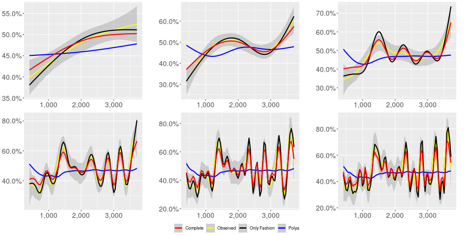
Figure 2: “Migration”, automated account subset: Sentiment curves for BOTs’ posts

Table 9: “10 days of traffic” dataset (Entire): MSE for different levels of smoothing

smooth	Only Fashion RP	Complete RP	Standard Pólya
no smooth	$2.32\times 10^{-1}$	$2.32\times 10^{-1}$	$2.33\times 10^{-1}$
k = 3	$\mathbf{3.15\times 10^{-9}}$	$2.61\times 10^{-7}$	$1.22\times 10^{-5}$
k = 5	$\mathbf{3.86\times 10^{-9}}$	$8.09\times 10^{-7}$	$3.34\times 10^{-5}$
k = 10	$\mathbf{1.94\times 10^{-8}}$	$2.02\times 10^{-6}$	$6.88\times 10^{-5}$
k = 20	$\mathbf{7.81\times 10^{-8}}$	$2.65\times 10^{-6}$	$8.80\times 10^{-5}$
k = 30	$\mathbf{1.74\times 10^{-7}}$	$2.86\times 10^{-6}$	$9.65\times 10^{-5}$
k = 50	$\mathbf{1.08\times 10^{-6}}$	$5.15\times 10^{-6}$	$1.53\times 10^{-4}$

Table 10: ”10 days traffic” dataset (only BOTs’ posts): MSE for different levels of smoothing

smooth	Only Fashion RP	Complete RP	Standard Pólya
no smooth	$2.31\times 10^{-1}$	$2.31\times 10^{-1}$	$2.31\times 10^{-1}$
k = 3	$\mathbf{4.10\times 10^{-7}}$	$6.67\times 10^{-7}$	$5.73\times 10^{-6}$
k = 5	$\mathbf{7.95\times 10^{-7}}$	$2.02\times 10^{-5}$	$5.97\times 10^{-5}$
k = 10	$\mathbf{6.81\times 10^{-6}}$	$2.35\times 10^{-5}$	$7.19\times 10^{-5}$
k = 20	$\mathbf{1.59\times 10^{-5}}$	$5.43\times 10^{-5}$	$1.52\times 10^{-4}$
k = 30	$\mathbf{2.59\times 10^{-5}}$	$5.98\times 10^{-5}$	$1.75\times 10^{-4}$
k = 50	$\mathbf{9.80\times 10^{-5}}$	$1.23\times 10^{-4}$	$3.49\times 10^{-4}$

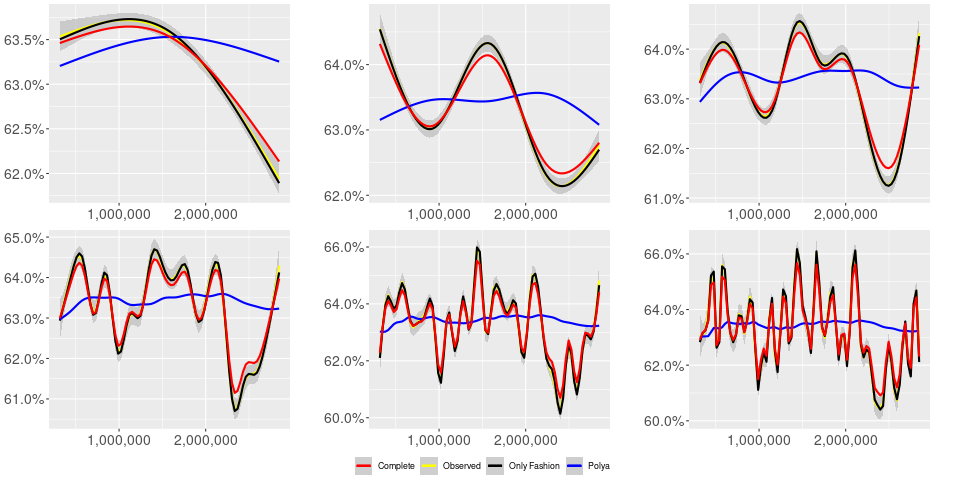
Figure 3: “10 days of traffic” dataset (Entire): Sentiment curves

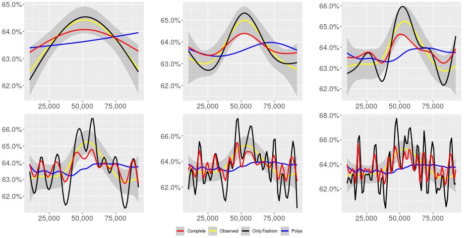
Figure 4: “10 days of traffic”, automated account subset: Sentiment curves for BOTs’ posts

Table 11: ”Covid” dataset (Entire): MSE for different levels of smoothing

smooth	Only Fashion RP	Complete RP	Standard Pólya
no smooth	$2.46\times 10^{-1}$	$2.46\times 10^{-1}$	$2.50\times 10^{-1}$
k = 3	$\mathbf{3.98\times 10^{-8}}$	$7.37\times 10^{-6}$	$2.58\times 10^{-3}$
k = 5	$\mathbf{5.51\times 10^{-8}}$	$7.53\times 10^{-6}$	$2.64\times 10^{-3}$
k = 10	$\mathbf{1.54\times 10^{-7}}$	$8.63\times 10^{-6}$	$2.92\times 10^{-3}$
k = 20	$\mathbf{7.93\times 10^{-7}}$	$9.37\times 10^{-6}$	$3.10\times 10^{-3}$
k = 30	$\mathbf{1.06\times 10^{-6}}$	$9.80\times 10^{-6}$	$3.24\times 10^{-3}$
k = 50	$\mathbf{2.06\times 10^{-6}}$	$1.10\times 10^{-5}$	$3.46\times 10^{-3}$

Table 12: ”Covid” dataset (only Bots’s posts): MSE for different levels of smoothing)

smooth	Only Fashion RP	Complete RP	Standard Pólya
no smooth	$2.45\times 10^{-1}$	$2.45\times 10^{-1}$	$2.49\times 10^{-1}$
k = 3	$\mathbf{3.23\times 10^{-6}}$	$5.33\times 10^{-5}$	$3.38\times 10^{-3}$
k = 5	$\mathbf{1.16\times 10^{-5}}$	$5.16\times 10^{-5}$	$3.38\times 10^{-3}$
k = 10	$\mathbf{2.84\times 10^{-5}}$	$6.88\times 10^{-5}$	$3.53\times 10^{-3}$
k = 20	$\mathbf{5.70\times 10^{-5}}$	$9.78\times 10^{-5}$	$3.80\times 10^{-3}$
k = 30	$\mathbf{1.67\times 10^{-4}}$	$1.81\times 10^{-4}$	$4.01\times 10^{-3}$
k = 50	$3.05\times 10^{-4}$	$\mathbf{2.94\times 10^{-4}}$	$4.38\times 10^{-3}$

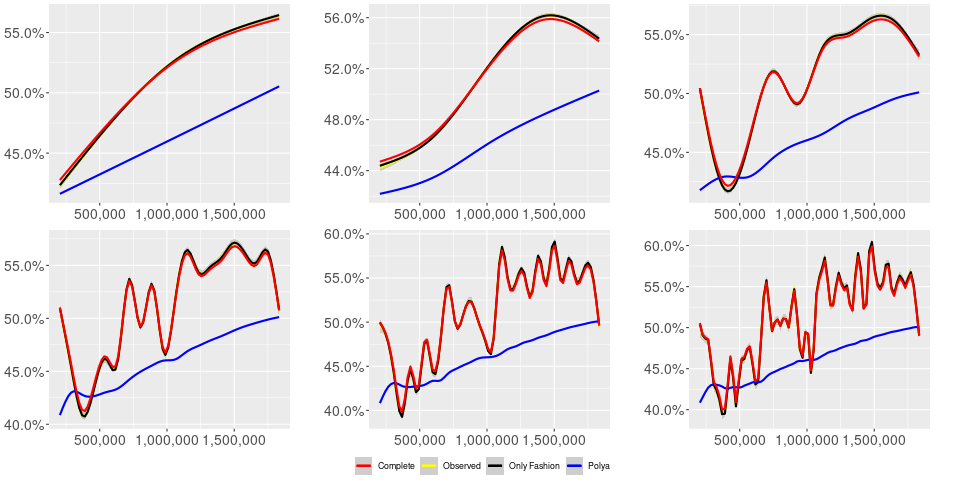
Figure 5: “Covid” dataset (Entire): Sentiment curves

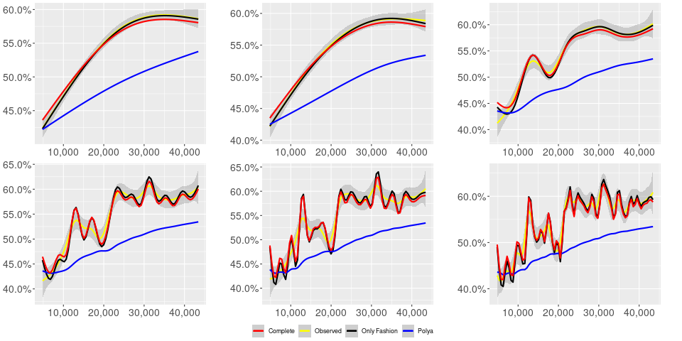
Figure 6: “Covid”, automated account subset: Sentiment curves for BOTs’ posts

4 Discussion and Conclusions

Online Social Networks (OSN) represent a perfect environment for the study of the emotional reaction to public events. It has been observed that the sentiment of a message may be a driver for the diffusion of a message in online social networks [5, 23, 6, 8]. Interestingly, Ref. [5] shows that, on different arguments, the sensitivity, i.e. the emotional reaction to the event, finds a sort of stability.

Leveraging on this feature of the online debate, we apply here a modification of the Pólya urn model, embedding a “local” reinforcement effect [1, 2], representing a sort of “fashion” contribution and capturing the persistence of a common sentiment. Similarly to the standard Pólya urn, the future outcome depends on the entire story, but, differently from the original model, in the Rescaled Pólya urn, the influence of the recent outcomes has a greater impact on future extractions. This represents the “fashion” effect and its introduction properly captures the evolution of the sentiment of the online debate. The results collected in Section 3 show that indeed the Rescaled Pólya model outperforms greatly the standard Pólya model. Moreover, the RP urn model permits to have reliable predictions from past observations: in particular, the model parameters are fitted using the data from all the previous slots, thus capturing a sensitivity to a certain emotional reaction for the argument, as in [5]. In this sense, when we focus on a single argument, as in the case of the Migration or Covid data sets, we have better results than when the argument is not specified, as in the case of 10 days traffic data set.

Summarising, the present paper has essentially two targets: to propose a novel model for the prediction of the sentiment in the online debate and to examine and study the implications of the Rescaled Pólya urn. Building a simple and realistic model improves our understanding of the phenomenon: in the particular case, the presence of a local reinforcement, i.e. the “fashion” effect described above, shows how persistent is the emotional reaction to a public event. It is worth to be mentioned that the application to Online Social Media is one of the possible applications of the proposed RP urn model: due to its abstractness and generality, it can be applied to any kind of phenomenon showing a local “fashion” behaviour. As it can be observed from the evolution of the model parameters, all of them converge smoothly to a fixed value. Estimating the parameters using only the closest slots, is going to be the target of near future research.

Declaration

Giacomo Aletti and Irene Crimaldi contributed to the theoretical definition of the Rescaled Pólya urn model; Fabio Saracco performed the data collection and cleaning; Giacomo Aletti performed the simulation; all the authors wrote, revised and approved the manuscript.

Acknowledgments

Giacomo Aletti is a member of the Italian Group “Gruppo Nazionale per il Calcolo Scientifico” of the Italian Institute “Istituto Nazionale di Alta Matematica” and Irene Crimaldi is a member of the Italian Group “Gruppo Nazionale per l’Analisi Matematica, la Probabilità e le loro Applicazioni” of the Italian Institute “Istituto Nazionale di Alta Matematica”. The authors acknowledge Fabio Del Vigna, Marinella Petrocchi and Manuel Pratelli for the bot detection on the above mentioned data sets.

Funding Sources

Irene Crimaldi and Fabio Saracco are supported by the Italian “Programma di Attività Integrata” (PAI), project “TOol for Fighting FakEs” (TOFFE) funded by IMT School for Advanced Studies Lucca. Fabio Saracco acknowledges also support from the European Project SoBigData++ GA. 871042

Appendix A Parameters evolution and choice

As it is mentioned in the main text, in order to fit the parameters of the model, we divided the entire dataset in time slots. Next, we use all slots previous to the one under consideration to fit the parameters. In this sense, we observe an evolution of the parameters as a matter of the evolution of the datasets, which is different when focusing on the different nature of users in the debate. Such a difference is particularly evident in the Migration debate. Human accounts show a nearly constant parameter dynamics: while $\beta$ is nearly constant in the Complete model, $\gamma^{*}$ and $p_{0}$ display a smooth slow variation of nearly the $10\%$ of their value, see Fig. 7. The dynamics of the parameters for automated accounts is completely different, see Fig. 8: in the Complete model, while $\beta$ is slowly decreasing (but still experiencing a much greater decrease than the one observed for human accounts), parameters $\gamma^{*}$ and $p_{0}$ display a step-like dynamics, ending shortly after $S=25$.

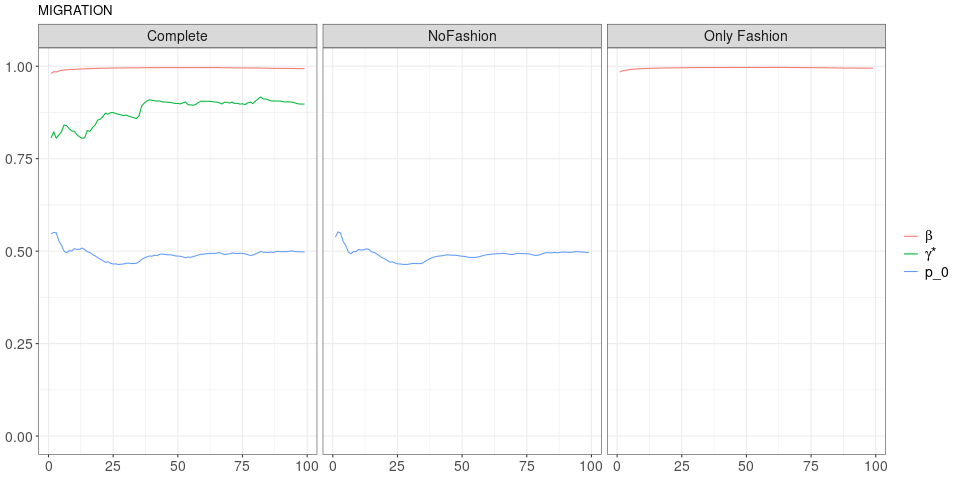
Figure 7: “Migration” dataset (Entire): Model parameters evolution. All parameters are slowly varying and converging to stable values.

Figure 8: “Migration” (only BOTs’ posts): Model parameters evolution. In the left panel, it is possible to distinguish an “Only fashion” initial phase ($\gamma^{*}\simeq 1$) and more balanced phase ($\gamma^{*}\in[0.5,0.75]$).

A similar, but less evident, dynamics can be observed in the “10 days of traffic” dataset, see Fig. 9 and 10: in this case, all parameters converge to 1 quite soon in the case of the entire dataset. Instead, we can see that $p_{0}$ converge, but to something more than 0.6 quite immediately for the social bot subset, while the value of $\gamma^{*}$ oscillates between 0.5 and 0, before converging to something less than 0.4. $\beta$ is nearly 1 for both cases.

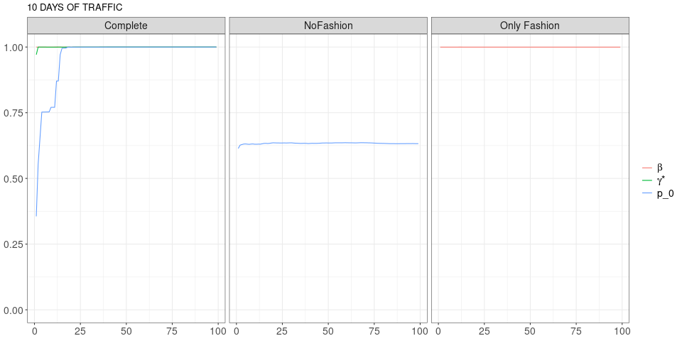
Figure 9: “10 days of traffic” dataset (Entire): Model parameters evolution. All parameters for the complete model converge to 1 quite soon. With $\gamma^{*}\simeq 1$, the Complete model is practically equivalent to the “Only Fashion” one.

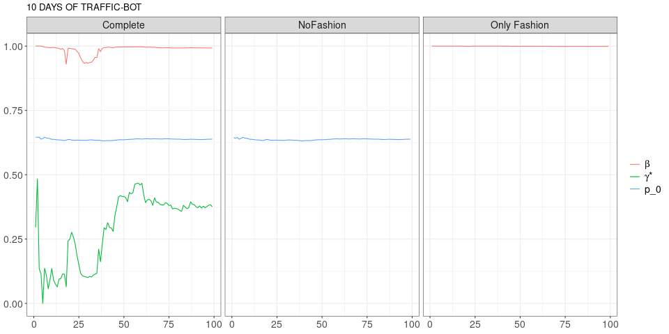
Figure 10: “10 days of traffic” (only BOTs’ posts): Model parameters evolution. Every parameter of the complete model, but $\gamma^{*}$, are essentially constant. Let us remark that $\gamma^{*}$ tunes the weight of the fashion process in the predictive mean.

In the case of the online debate during the COVID-19 epidemic, Fig.s 11 and 12, the differences are extremely low, with the values of $\gamma^{*}$ quite flickering before converging to a value little lower than the one obtained for the entire dataset. All other parameters are quite similar, both in the value and in the dynamics.

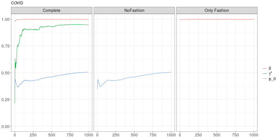
Figure 11: “Covid” dataset (Entire): Model parameters evolution. All parameters are nearly constant or slowly converging. This slow convergence is probably due to the fact that the fit of the parameters is mostly driven by the long range history. In the case of the “COVID” dataset, $S=1000$.

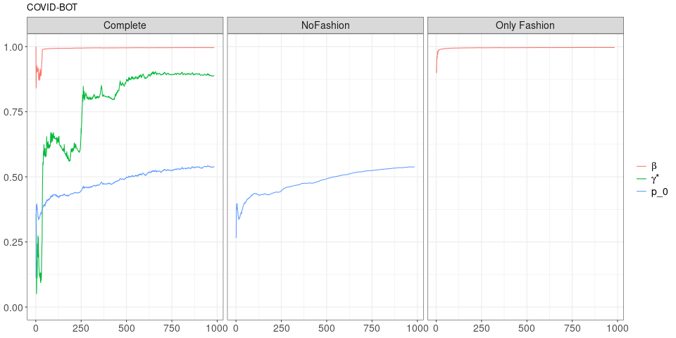
Figure 12: “Covid” dataset (Only BOTs’ posts): Model parameters evolution. Differently to the other datasets, the parameters evolution for the Bots’ posts follows the one for the entire dataset, displaying a greater noise contribution for $\gamma^{*}$. In the case of the “Covid” dataset, $S=1000$.

Actually, it is not clear if this evolution of the parameters for the BOT subset is due to the limited numerosity of the dataset or to an indeed different dynamics. This issue is not the focus of this work and it is going to be the target of further analyses.

References

- [1] Aletti, G. & Crimaldi, I. The rescaled Pólya urn: local reinforcement and chi-squared goodness of fit test. arXiv:1906.10951 (2019).
- [2] Aletti, G. & Crimaldi, I. Generalized rescaled Pólya urn and its statistical applications. arXiv:2010.06373 (2020).
- [3] Publication Office of the European Union. Media use in the European Union (2018).
- [4] Mitchell, A. & Page, D. The evolving role of news of Twitter and Facebook. Tech. Rep., Pew Research Center (2015).
- [5] Zollo, F. et al. Emotional dynamics in the age of misinformation. PLoS One 10 (2015). 1505.08001.
- [6] Del Vicario, M. et al. Echo Chambers: Emotional Contagion and Group Polarization on Facebook. Sci. Rep. (2016). 1607.01032.
- [7] Del Vicario, M. et al. Echo Chambers: Emotional Contagion and Group Polarization on Facebook. Sci. Rep. (2016). 1607.01032.
- [8] Zollo, F., Sluban, B., Mozetič, I. & Quattrociocchi, W. Toward a better understanding of emotional dynamics on Facebook. In Stud. Comput. Intell. (2018).
- [9] Bradshaw, S. & Howard, P. The global organization of social media disinformation campaigns. Journal of International Affairs 71 (2017).
- [10] Bradshaw, S. & Howard, P. The global disinformation order: 2019 global inventory of organised social media manipulation. Tech. Rep., Oxford, UK: Project on Computational Propaganda (2019).
- [11] National Endowment for Democracy. Issue brief: Distinguishing disinformation from propaganda, misinformation, and “fake news”. URL https://www.ned.org/issue-brief-distinguishing-disinformation-from-propaganda-misinformation-and-fake-news/.
- [12] Cresci, S., Di Pietro, R., Petrocchi, M., Spognardi, A. & Tesconi, M. Fame for sale: Efficient detection of fake Twitter followers. Decis. Support Syst. (2015). 1509.04098.
- [13] Ferrara, E., Varol, O., Davis, C., Menczer, F. & Flammini, A. The rise of social bots. Commun. ACM 59, 96–104 (2016).
- [14] Shao, C. et al. The spread of low-credibility content by social bots. Nat. Commun. 9, 4787 (2018). 1707.07592.
- [15] Stella, M., Ferrara, E. & Domenico, M. D. Bots sustain and inflate striking opposition in online social systems. PNAS 115, 12535–12440 (2018).
- [16] Yang, K. C. et al. Arming the public with artificial intelligence to counter social bots. Hum. Behav. Emerg. Technol. (2019). 1901.00912.
- [17] Cresci, S., Spognardi, A., Petrocchi, M., Tesconi, M. & Pietro, R. D. The paradigm-shift of social spambots: Evidence, theories, and tools for the arms race. In 26th Int. World Wide Web Conf. 2017, WWW 2017 Companion (2019). 1701.03017.
- [18] Caldarelli, G., De Nicola, R., Del Vigna, F., Petrocchi, M. & Saracco, F. The role of bot squads in the political propaganda on Twitter. Commun. Phys. 3, 1–15 (2020). 1905.12687.
- [19] Flaxman, S., Goel, S. & Rao, J. M. Filter Bubbles, Echo Chambers, and Online News Consumption. Public Opinion Quarterly 80, 298–320 (2016).
- [20] Becatti, C., Caldarelli, G., Lambiotte, R. & Saracco, F. Extracting significant signal of news consumption from social networks: the case of Twitter in Italian political elections. Palgrave Commun. (2019). 1901.07933.
- [21] Pacheco, D. et al. Uncovering coordinated networks on social media (2020). 2001.05658.
- [22] Caldarelli, G., de Nicola, R., Petrocchi, M., Pratelli, M. & Saracco, F. Analysis of online misinformation during the peak of the covid-19 pandemics in italy (2020). 2010.01913.
- [23] Qiu, X., Oliveira, D. F., Sahami Shirazi, A., Flammini, A. & Menczer, F. Limited individual attention and online virality of low-quality information. Nat. Hum. Behav. 1 (2017). 1701.02694.
- [24] Jansen, B. J., Zhang, M., Sobel, K. & Chowdury, A. Twitter power: Tweets as electronic word of mouth. J. Am. Soc. Inf. Sci. Technol. 60, 2169–2188 (2009).
- [25] AGCOM. Report on the consumption of information. Tech. Rep. February, Autorità per le Garanzie delle Comunicazioni (2018).
- [26] Ren, F. & Wu, Y. Predicting user-topic opinions in twitter with social and topical context. IEEE Transactions on Affective Computing 4, 412–424 (2013).
- [27] Chakraborty, K., Bhattacharyya, S. & Bag, R. A survey of sentiment analysis from social media data. IEEE Transactions on Computational Social Systems 7, 450–464 (2020).
- [28] Patil, H. P. & Atique, M. Sentiment analysis for social media: A survey. In 2015 2nd International Conference on Information Science and Security (ICISS), 1–4 (2015).
- [29] Yue, L., Chen, W., Li, X., Zuo, W. & Yin, M. A survey of sentiment analysis in social media. Knowl Inf Syst 60, 617–663 (2019).
- [30] Bing, L., Chan, K. C. C. & Ou, C. Public sentiment analysis in twitter data for prediction of a company’s stock price movements. In 2014 IEEE 11th International Conference on e-Business Engineering, 232–239 (2014).
- [31] Bollen, J., Mao, H. & Zeng, X. Twitter mood predicts the stock market. Journal of Computational Science 2, 1 – 8 (2011). URL http://www.sciencedirect.com/science/article/pii/S187775031100007X.
- [32] Golder, S. A. & Macy, M. W. Diurnal and seasonal mood vary with work, sleep, and daylength across diverse cultures. Science 333, 1878–1881 (2011). URL https://science.sciencemag.org/content/333/6051/1878. https://science.sciencemag.org/content/333/6051/1878.full.pdf.
- [33] Lei, X., Qian, X. & Zhao, G. Rating prediction based on social sentiment from textual reviews. IEEE Transactions on Multimedia 18, 1910–1921 (2016).
- [34] O’Connor, B., Balasubramanyan, R., Routledge, B. & Smith, N. From tweets to polls: Linking text sentiment to public opinion time series. In International AAAI Conference on Weblogs and Social Media, vol. 11 (2010).
- [35] Tumasjan, A., Sprenger, T., Sandner, P. & Welpe, I. Predicting elections with twitter: What 140 characters reveal about political sentiment. In Word. Journal Of The International Linguistic Association, vol. 10 (2010).
- [36] Yu, X., Liu, Y., Huang, X. & An, A. Mining online reviews for predicting sales performance: A case study in the movie domain. IEEE Transactions on Knowledge and Data Engineering 24, 720–734 (2012).
- [37] Zhu, J., Wang, H., Zhu, M., Tsou, B. & Ma, M. Aspect-based opinion polling from customer reviews. Affective Computing, IEEE Transactions on 2(1), 37 – 49 (2011).
- [38] Chmiel, A. et al. Collective emotions online and their influence on community life. PLOS ONE 6, 1–8 (2011). URL https://doi.org/10.1371/journal.pone.0022207.
- [39] Bollen, J., Pepe, A. & Mao, H. Modeling public mood and emotion: Twitter sentiment and socio-economic phenomena. Computing Research Repository - CORR (2009).
- [40] Tan, S. et al. Interpreting the public sentiment variations on twitter. IEEE Transactions on Knowledge and Data Engineering 26, 1158–1170 (2014).
- [41] Kursuncu, U. et al. Predictive analysis on twitter: Techniques and applications. ArXiv abs/1806.02377 (2018).
- [42] Chadwick, A. The hybrid media system: Politics and power, second edition (Oxford University Press, New York [etc.], 2017).
- [43] Zaman, T., Fox, E. B. & Bradlow, E. T. A bayesian approach for predicting the popularity of tweets. Ann. Appl. Stat. (2014). 1304.6777.
- [44] Dow, P. A., Adamic, L. A. & Friggeri, A. The anatomy of large facebook cascades. In Proc. 7th Int. Conf. Weblogs Soc. Media, ICWSM 2013 (2013).
- [45] Kumar, R., Mahdian, M. & McGlohon, M. Dynamics of conversations. In Proc. ACM SIGKDD Int. Conf. Knowl. Discov. Data Min. (2010).
- [46] Kobayashi, R. & Lambiotte, R. TiDeH: Time-dependent Hawkes process for predicting retweet dynamics. In Proc. 10th Int. Conf. Web Soc. Media, ICWSM 2016 (2016). 1603.09449.
- [47] Gao, S., Ma, J. & Chen, Z. Modeling and predicting retweeting dynamics on microblogging platforms. In WSDM 2015 - Proc. 8th ACM Int. Conf. Web Search Data Min. (2015).
- [48] Golosovsky, M. & Solomon, S. Stochastic dynamical model of a growing citation network based on a self-exciting point process. Phys. Rev. Lett. (2012).
- [49] Zhao, Q., Erdogdu, M. A., He, H. Y., Rajaraman, A. & Leskovec, J. SEISMIC: A self-exciting point process model for predicting tweet popularity. In Proc. ACM SIGKDD Int. Conf. Knowl. Discov. Data Min. (2015).
- [50] Eggenberger, F. & Pólya, G. Über die statistik verketteter vorgänge. ZAMM - Journal of Applied Mathematics and Mechanics / Zeitschrift für Angewandte Mathematik und Mechanik 3, 279–289 (1923). URL https://onlinelibrary.wiley.com/doi/abs/10.1002/zamm.19230030407. https://onlinelibrary.wiley.com/doi/pdf/10.1002/zamm.19230030407.
- [51] Mahmoud, H. M. Pólya urn models. Texts in Statistical Science Series (CRC Press, Boca Raton, FL, 2009).
- [52] Pemantle, R. A survey of random processes with reinforcement. Probab. Surveys 4, 1–79 (2007). URL https://doi.org/10.1214/07-PS094.
- [53] Tang, J. et al. Quantitative study of individual emotional states in social networks. Affective Computing, IEEE Transactions on 3 (2012).
- [54] Aletti, G., Crimaldi, I. & Ghiglietti, A. Synchronization of reinforced stochastic processes with a network-based interaction. Ann. Appl. Probab. 27, 3787–3844 (2017). URL https://doi.org/10.1214/17-AAP1296.
- [55] Aletti, G., Crimaldi, I. & Ghiglietti, A. Interacting reinforced stochastic processes: Statistical inference based on the weighted empirical means. Bernoulli 26, 1098–1138 (2020).
- [56] Aletti, G., Ghiglietti, A. & Rosenberger, W. F. Nonparametric covariate-adjusted response-adaptive design based on a functional urn model. Ann. Statist. 46, 3838–3866 (2018). URL https://doi.org/10.1214/17-AOS1677.
- [57] Aletti, G., Ghiglietti, A. & Vidyashankar, A. N. Dynamics of an adaptive randomly reinforced urn. Bernoulli 24, 2204–2255 (2018). URL https://doi.org/10.3150/17-BEJ926.
- [58] Berti, P., Crimaldi, I., Pratelli, L. & Rigo, P. Asymptotics for randomly reinforced urns with random barriers. J. Appl. Probab. 53, 1206–1220 (2016). URL https://doi.org/10.1017/jpr.2016.75.
- [59] Caldarelli, G., Chessa, A., Crimaldi, I. & Pammolli, F. Weighted networks as randomly reinforced urn processes. Phys. Rev. E 87, 020106 (2013). URL https://link.aps.org/doi/10.1103/PhysRevE.87.020106.
- [60] Chen, M.-R. & Kuba, M. On generalized pólya urn models. J. Appl. Probab. 50, 1169–1186 (2013). URL https://doi.org/10.1239/jap/1389370106.
- [61] Collevecchio, A., Cotar, C. & LiCalzi, M. On a preferential attachment and generalized pólya’s urn model. Ann. Appl. Probab. 23, 1219–1253 (2013). URL https://doi.org/10.1214/12-AAP869.
- [62] Crimaldi, I. Central limit theorems for a hypergeometric randomly reinforced urn. J. Appl. Probab. 53, 899–913 (2016). URL https://doi.org/10.1017/jpr.2016.48.
- [63] Ghiglietti, A., Vidyashankar, A. N. & Rosenberger, W. F. Central limit theorem for an adaptive randomly reinforced urn model. Ann. Appl. Probab. 27, 2956–3003 (2017). URL https://doi.org/10.1214/16-AAP1274.
- [64] Laruelle, S. & Pagés, G. Randomized urn models revisited using stochastic approximation. Ann. Appl. Proba. 23, 1409–1436 (2013).
- [65] Lasmar, N., Mailler, C. & Selmi, O. Multiple drawing multi-colour urns by stochastic approximation. J. Appl. Probab. 55, 254–281 (2018).
- [66] Chen, Y. & Skiena, S. Building sentiment lexicons for all major languages. In Proceedings of the 52nd Annual Meeting of the Association for Computational Linguistics (Short Papers), 383–389 (2014).