TiDeH: Time-Dependent Hawkes Process for Predicting Retweet Dynamics

Abstract

Online social networking services allow their users to post content in the form of text, images or videos. The main mechanism driving content diffusion is the possibility for users to re-share the content posted by their social connections, which may then cascade across the system. A fundamental problem when studying information cascades is the possibility to develop sound mathematical models, whose parameters can be calibrated on empirical data, in order to predict the future course of a cascade after a window of observation. In this paper, we focus on Twitter and, in particular, on the temporal patterns of retweet activity for an original tweet. We model the system by Time-Dependent Hawkes process (TiDeH), which properly takes into account the circadian nature of the users and the aging of information. The input of the prediction model are observed retweet times and structural information about the underlying social network. We develop a procedure for parameter optimization and for predicting the future profiles of retweet activity at different time resolutions. We validate our methodology on a large corpus of Twitter data and demonstrate its systematic improvement over existing approaches in all the time regimes.

I Introduction

In recent years, online social networking sites (OSNs) have become an increasingly central medium for information diffusion. In OSNs, users can generate their own content, but also discover information generated by their social contacts and re-share it to their own contacts. Importantly, an information can be re-shared multiple times, and the resulting multiplicative mechanism may lead to cascades over a large number of people, possibly even reaching regions of the social graph distant from the original post Kwak et al. (2010). Such cascades have been identified in a variety of OSNs, including Facebook and Twitter Dow et al. (2013); Kumar et al. (2010).

A growing body of research has improved our understanding of information cascades, from the design of accurate theoretical models for diffusion Easley and Kleinberg (2010); Goetz et al. (2009); Centola (2010), to the empirical study of the structural properties of cascades Adar and Adamic (2005); Gruhl et al. (2004); Salah-Brahim et al. (2012) and of their interplay with the structure of the underlying topology Weng et al. (2014). From a practical point of view, a crucial question is to predict the future evolution of an information cascade, based on observations made during its early stage. The most simple way to formulate this problem is to predict the final size of the information cascade, that is the total number of direct and indirect re-shares received by a given post. This prediction problem has important applications for the good-functioning of OSNs, for instance to rank content and improve the presentation of information to often overflowed users, and for media campaign management. In a machine learning framework, this problem can be solved as a classification task, where an exhaustive set of features, including semantic, structural and temporal information, are fed into standard classification methods Petrovic et al. (2011); Hong et al. (2011); Bao et al. (2013); Cheng et al. (2014). An alternative approach consists in building realistic, yet simple and principled, models of information diffusion, and fitting their parameters on empirical data Zaman et al. (2014); Gao et al. (2015); Zhao et al. (2015). This modeling approach has the advantage of improving our understanding of the mechanisms driving diffusion, and of testing the predictive power of information diffusion models.

Present work: In this paper, we extend the classical problem of cascade size prediction and aim at predicting how the cascade size evolves in time. In practice, we focus on Twitter and on the number of retweets of an original tweet, but our method is general and can be applied to any type of OSN. Our problem is the following: given a time series of retweets during a window of observation, being able to predict the time evolution of the frequency at which retweets will appear in the future, at different temporal resolutions. We are thus interested in predicting not only a number, the final size of the cascade, but a curve, how popularity will evolve in time, after a window of observation. To do so, we adopt a modeling perspective and see the time series as a Time-Dependent Hawkes process, TiDeH, which generalizes a classical model for self-exciting point processes. Hawkes process differ from memoryless Poisson processes as the future rate of activity is boosted by the occurrence of previous events Hawkes (1971). They can themselves be seen as generalizations of epidemiological models and branching processes Newman (2010), where an additional ingredient is incorporated, a memory kernel determining the time between a cause, e.g. a tweet, and its effect, a retweet. Hawkes processes have been adopted in a wide range of applications, including information diffusion in OSNs Zhao et al. (2015), where their multiplicative nature naturally translates the fact that a new re-share exposes new followers and may thus provoke new re-shares in the future. Here, we additionally make the Hawkes process time-dependent by allowing the model parameter to vary daily.

Our methodology is set up as follows: for a tweet of interest, we observe its retweet sequence $\{t_{i},d_{i}\}$ up to time $t_{0}+T$, where $t_{i}$ is the $i$-th retweeted time, $d_{i}$ is the number of followers of the $i$-th retweeting person, $t_{0}$ is the posted time of the original tweet, $d_{0}$ is the number of followers of the tweeting person, and $T$ is the duration of the observation. We first fit the parameters of TiDeH based on time series of retweets and information on the number of followers. We then predict retweet activity, defined as the number of retweets in the $k$-th bin $t\in[(k-1)\Delta_{\rm pred},k\Delta_{\rm pred}\}$, where $\Delta_{\rm pred}$ is the bin width that represents the time resolution of the prediction (Fig. 1). Let us note here that our prediction task generalizes the task of predicting the total number of retweets, as the latter is recovered either for large values of $\Delta_{\rm pred}$ or by summing all of the future values of retweet activity. The prediction of future events is performed by solving numerically a self-consistent integral equation of the model during the prediction period. As we will see, TiDeH presents a series of advantages over existing approaches, as it significantly improves the accuracy of predictions and that it provides a systematic, mathematically sound, framework to predict temporal variations of re-shares in OSNs.

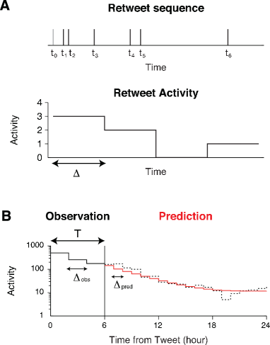
Figure 1: Predicting retweet activity. A. Top: Retweet sequence. Black (Grey) bars represent the retweet (original tweet) times. Bottom: Retweet activity. Retweet activity is defined by the number of retweet in a time window. The duration of the time bin $\Delta$ determines the temporal resolution of the analysis. B. Prediction problem. We aim to predict the future retweet activity from observed retweet times and number of followers up to time $t_{0}+T$. In general, two different types of binning, $\Delta_{\rm obs}$ and $\Delta_{\rm pred}$, can be used for the estimation of model parameters and for the prediction of future events.

The rest of the paper is organized as follows: Section 2 surveys the related work. In Section 3, we describe the data-set, describe TiDeH, and provide evidence for the circadian dependence of the model parameter. We then devise an optimization method for parameter estimation and test it on artificial data. In section 4, we present our procedure to predict the future profiles of retweet activity and compare the accuracy of different versions of TiDeH. In section 5, we thoroughly evaluate our method on empirical data and compare its performance with state-of-the-art approaches. In Section 6, we conclude and discuss future research directions.

II Related work

The study of information cascades in OSNs is an active field of research Rogers (2010). Many papers have analyzed and described the temporal and structural properties of empirical information cascades Dow et al. (2013); Kumar et al. (2010). In parallel, theoretical works have considered the design of theoretical models of cascade dynamics in networks Easley and Kleinberg (2010). Our work is at the interface between these approaches, as the prediction of the future course of a cascade is performed through a properly calibrated information diffusion model. The problem of cascade prediction is generally defined to estimate the final size of a cascade, or equivalently the total popularity of an original post. Broadly speaking, two types of methods have been developed to solve this problem. On the one hand, machine learning methods consist in collecting an exhaustive list of potentially relevant features for each cascade, including semantic content, meta-information, structural and temporal features. Learning or statistical methods are then applied in order to classify the cascades and predict their future size. Following the seminal observation that popularity on early days and later ones are high log-linear correlated Szabo and Huberman (2010), more recent works focusing on Twitter include Petrovic et al. (2011), where learning techniques are shown to achieve similar performance to humans, but also Yang and Counts (2010) showing that the number of username mentions helps predicting the speed and shape of retweet dynamics. In the case of re-shares on Facebook, let us also mention Cheng et al. (2014) where the authors observe that temporal and structural features of cascades are key predictors for their growth. Known drawbacks of this family of methods include a high sensitivity to the quality of the features, the requirement of an extensive training, and thus a limited applicability in real-time online settings Bandari et al. (2012).

A second type of predictive methods aims at calibrating models of information diffusion on time series of events during a window of observation, possibly by incorporating additional social network information. Two important ingredients of the models are the instantaneous character of events in OSNs, which are thus so-called “point processes” in the mathematical literature, and the multiplicative nature of the diffusion, as new events tend to trigger new ones. For these reasons, several works have developed models based on self-exciting point processes and, in particular, Hawkes processes. A major distinction between our model and existing ones Zaman et al. (2014); Yang and Zha (2013) is its time-dependence as we take into account circadian rhythms of online popularity and aging of information. Importantly, the infectiousness of the original tweet naturally depends on its posting time, in agreement with observations that it is an intuitive predictor for popularity Petrovic et al. (2011), and this effect is also present for later retweets. Our model can be seen as a time-dependent extension of SEISMIC Zhao et al. (2015), as our model also incorporates a partial information of the network structure, but with two additional differences. First, our goal is to predict the time evolution of the number of retweets in the future, and not simply the total number of retweets. As we show below, the incorporation of circadian patterns is particularly important to improve accuracy in this context. Second, we develop a framework for predicting future activity that is mathematically consistent with the modeling. Our model is also related to the time-dependent Poisson process model Gao et al. (2015), which we compare to TiDeH below, and to SpikeM Matsubara et al. (2012), which incorporates daily cycles and a finite population ensuring an asymptotic decay of the propagation, but differs from our approach by its deterministic and descriptive character. These two models also have the drawback of neglecting the effect of social network topology on information cascade, despite its important impact in spreading processes.

Beyond these works on information diffusion, it is important to emphasize here that Hawkes processes have been applied in a variety of settings in order to describe and to predict univariate or multivariate data. Originally defined to describe earthquake dynamics Hawkes (1971), where a power-law memory kernel was first introduced Ogata (1988), it was for instance applied to predict where and when aftershocks would occur Helmstetter and Sornette (2003). In finance, and in particular high frequency finance Bacry et al. (2015), estimations of the model parameters allow to quantify if price changes are dominated by endogenous feedback processes, as opposed to exogenous news Filimonov and Sornette (2012). Similar applications have also been developed to model popularity of online content, in particular in Youtube Crane and Sornette (2008), by estimating the different types of response after endogenous and exogenous bursts of activity. In social dynamics, Masuda et al. (2013) showed that the model can help reproduce empirical features observed in conversation event sequences, and Mohler et al. (2011) applied it in order to predict criminal events. In scientometrics, citation dynamics have been also modeled by modified Hawkes models Golosovsky and Solomon (2012), and future citations of a given paper predicted by reinforced Poisson process Shen et al. (2014). Finally, let us also note that Hawkes processes have also triggered theoretical research associated to the non-Markovian nature of their dynamics, and its impact on spreading times Delvenne et al. (2015).

III Modeling retweet activity via time-dependent Hawkes Process

III.1 Data sets

We analyzed 166,076 tweets on Twitter from October 7 to November 7, 2011, which was used in a previous study Zhao et al. (2015) and available in http://snap.stanford.edu/seismic/. For each tweet, the dataset includes tweet ID, posting time, time of retweets, and the number of followers of users for the original tweet and later retweets. The retweet times are recorded up to 7 days (168 hours) from the original post for each tweet. Note that the data contains some minimal information about the network structure (the number of followers), as it is easily available through the Twitter API, but the presence of connections between users in the Twitter network is not known. We focus on a subset of popular tweets (738 tweets) that have at least 2,000 retweets in order to calibrate our model and to evaluate the performance of our predictions.

III.2 TiDeH: Time-dependent Hawkes process

We develop a Time-Dependent Hawkes process (TiDeH) for predicting retweet activity, and extending the classical stationary Hawkes process Hawkes (1971); Zhao et al. (2015) (Fig. 2). The probability for getting a retweet in a small time interval $[t,t+\Delta t]$ is described as

$$\textrm{Prob}\left(\textrm{Getting a retweet in }\ [t,t+\Delta t]\right)=\lambda(t)\Delta t,$$ (1)

where the time-dependent rate depends on previous events as

$$\lambda(t)=p(t)\sum_{i:t_{i}<t}d_{i}\phi(t-t_{i}),$$ (2)

and where $p(t)$ is the infectious rate, $t_{i}$ is the time of $i$-th retweet. Following Zhao et al. (2015), we also incorporate the number $d_{i}$ of followers of the $i$-th retweeting person. By doing so, the model essentially generates a branching process for the diffusion, and gives more importance to highly connected nodes. This step is akin to tree-like and heterogeneous mean-field approximations popular to simplify the theoretical study of epidemic spreading on networks Newman (2010). The memory kernel $\phi(s)$ is a probability distribution for the reaction time of a follower, that is the time interval between a tweet by the followee and its retweet by the follower. This distribution has been shown to be heavily tailed in a variety of social networks Vázquez et al. (2006); Crane and Sornette (2008), and it is fitted to the empirical data by the function

$$\phi(s)=\begin{cases}0&(s<0)\\ c_{0}&(0\leq s\leq s_{0})\\ c_{0}(s/s_{0})^{-(1+\theta)}&(\textrm{Otherwise})\\ \end{cases},$$ (3)

The parameters were set to $c_{0}=6.49\times 10^{-4}$ (/seconds), $s_{0}=300$ seconds, and $\theta=0.242$ Zhao et al. (2015). As we show in the following section, $p(t)$ is observed to decrease to zero for sufficiently long times, which ensures that the predicted number of retweets does not diverge.

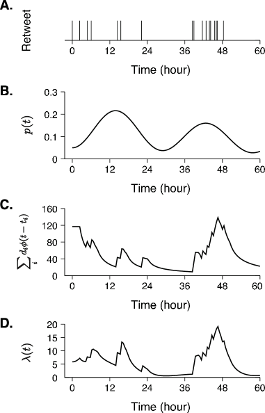
Figure 2: Time-dependent Hawkes process. A. Simulated retweet activity. The original tweet (time 0) and retweet times are represented as a bar. B. Infectious rate $p(t)$ (1st term of Eq. 2). C. Memory Effect $\sum_{i}d_{i}\phi(t-t_{i})$ (2nd term of Eq. 2). D. Instantaneous probability of a retweet $\lambda(t)$, as obtained by the product of B and C.

III.3 Modeling the infectious rate of a tweet

III.3.1 Estimating the instantaneous infectious rate.

The infectious rate $p(t)$ is estimated by using moving time windows. Assuming that the infectious rate is constant in a small time window $t\in[t_{\textrm{st}},t_{\textrm{en}}]$, $p(t)$ is calculated by the maximum likelihood method,

$$\hat{p}_{t}=\frac{\delta R}{\sum_{i}n_{i}\{\Phi(t_{\textrm{en}}-t_{i})-\Phi(t_{i}-t_{\textrm{st}})\}},$$ (4)

where $\delta R$ is the number of retweets in the time window and $\Phi(t)$ is the integral of the memory kernel, $\Phi(t)=\int_{0}^{t}\phi(s)ds$. Note that alternative methods could be applied, without the need for moving time windows, for instance by using the empirical Bayes method Koyama and Shinomoto (2005). However, our choice is motivated by its simplicity and the window size ($\Delta_{\rm obs}=t_{\textrm{en}}-t_{\textrm{st}}$) is set to 4 hours. Examples of the estimated infectious rate from a retweet sequence are shown in Figure 3.

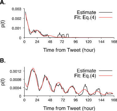
Figure 3: Estimated infectious rate from two retweet sequences. Two types of dynamics are observed, i.e., a decay (A) and a decay with circadian oscillations (B). Black lines are the rates estimated by the moving time window and red lines indicate the fit by the proposed model.

III.3.2 Modeling the infectious rate of retweets.

Infectious rates $p(t)$ from a retweet sequence (Fig. 3) clearly show two properties, a circadian cycles and a slow decay. The decay is expected due to the inevitable aging of information, whose life-cycle is known to be short in microblogging systems, but also to the decreasing number of potentially interested followers, as the cascade progresses. The oscillations are expected for cascades that remain geographically localized, within a limited number of time zones, such that daily cycles of human activity naturally translate into cycles of retweet activity. Based on this observation, we propose a minimal model for the time dependence of the infectious rate

$$p(t)=p_{0}\left\{1-r_{0}\sin\left(\frac{2\pi}{T_{m}}(t+\phi_{0})\right)\right\}e^{-(t-t_{0})/\tau_{m}}$$ (5)

where, as before, $t_{0}$ is the time of the original tweet. The period of oscillation is set to $T_{m}=1$ day. The parameters, $p_{0},r_{0},\phi_{0},\tau_{m}$ correspond to the intensity, the relative amplitude of the oscillation, its phase, and the characteristic time of popularity decay respectively. These four parameters are fitted by minimizing the least square error

$$E_{p}=\sum_{k=1}^{M}\{\hat{p}_{k}-p((k+0.5)\Delta_{\rm obs})\}^{2},$$ (6)

where $M=T/\Delta_{\rm obs}$ is the number of bins, and $\hat{p}_{k}$ is the estimate of the infectious rate in a time bin $t\in[k\Delta_{\rm obs},(k+1)\Delta_{\rm obs}]$. The Levenberg$-$Marquardt algorithm is then used to minimize the error, and the parameter range of $r$ and $\tau_{m}$ is restricted, i.e., $-1<r<1$ and $0.5<\tau_{m}<20$ days.

III.3.3 Validation of the fitting procedure on synthetic data.

We validate the fitting procedure for $(p_{0},r_{0},\phi_{0},\tau_{m})$ by analyzing synthetic data generated by TiDeH (1,2) with the time-dependent infectious rate (5). The number of followers $d_{i}$ was obtained from a retweet sequence of the empirical data. Figure 4 shows that the fitting procedure, when applied to one retweet sequence, can reconstruct the unobservable infectious rate from the simulated sequence. We evaluate the accuracy of the parameter estimation by comparing its estimates with the “ground-truth” values used to generate the synthetic data. Table 1 summarizes the mean and standard deviation of the estimates for 100 trials. The relative errors are 0.0 %, 1.9 %, 9.6%, and 1.0 %, for $p_{0}$, $r_{0}$, $\phi_{0}$, and $\tau_{m}$, respectively, suggesting that the fitting procedure accurately reconstructs the parameters for sufficiently long observation period, here set to $T=$ 2 days.

Table 1: Parameter estimation by the least square method from simulated data (observation time $T$: 2 days ).

Parameter	Estimate	True
$p_{0}$	${\bf 0.001\pm 0.00009}$	$0.001$
$r_{0}$	${\bf 0.416\pm 0.069}$	$0.424$
$\phi_{0}$	${\bf 0.113\pm 0.030}$	$0.125$
$\tau_{m}$	${\bf 2.02\pm 0.66}$	$2.00$

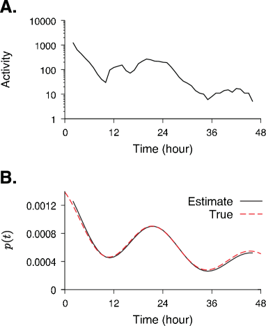
Figure 4: Estimating the infectious rate $p(t)$ from synthetic data. A. Activity of simulated data. The number of events in two hours window is counted. B. Fitted infectious rate. The rate of the model with optimized parameters (black) is compared to the true rate (red dashed).

As a next step, we examine the dependence of the estimation accuracy on the duration of the observation period. Fig. 5 shows that accuracy deteriorates for short durations. In particular, we cannot obtain reliable estimates for the phase $\phi_{0}$ and the time constant $\tau_{m}$ if the observation time is shorter than 24 hours. A possible reason for this lack of accuracy is that there are too many parameters to be estimated from limited data. To test this hypothesis, we consider the situation when only the amplitude parameter $p_{0}$ is to be fitted, while the other parameters ($r_{0},\phi_{0},\tau_{m}$) are known. In that case, $p_{0}$ can be accurately estimated, even from a very short observation window, $T=1$ hour (Fig. 6).

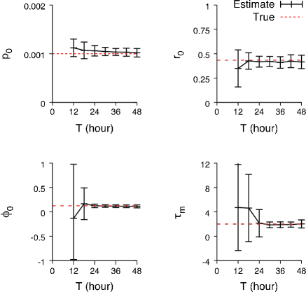
Figure 5: Dependence of the accuracy of parameter estimation on the observation time $T$. The mean and standard deviation of the estimates are calculated from 100 synthetic data.

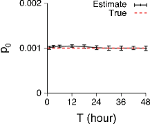
Figure 6: Dependence of the accuracy of parameter estimation on the observation time $T$: case when only $p_{0}$ is unknown.

IV Predicting future retweet activity via TiDeH

We develop a procedure to predict the future retweet activity of an original tweet based on TiDeH. It consists in two steps. First, the infectious rate $p(t)$ is calibrated. Second, the future retweet rate $\lambda(t)$ is calculated based on the infectious rate and the observed retweet sequence $\{t_{i},d_{i}\}$ $(t_{i}<T)$, and the future retweet activity is estimated.

IV.1 Step 1: Fitting the infectious rate $p(t)$

We consider three ways to identify the infectious rate $p(t)$ from a retweet sequence. In a first approach, we assume that the infectious rate is constant $p(t)=p_{0}$ and this single parameter is estimated from the observed retweet sequence by the maximum likelihood method (4). In a second approach, we consider the model (5) for the time-varying infectious rate, and all the parameters $(p_{0},r_{0},\phi_{0},\tau_{m})$ are estimated from the observed retweet sequence by using the fitting procedure developed in section III.3. In a third approach, we again adopt (5) for the time-varying infectious rate, but we now optimize the shape parameters $(r_{0},\phi_{0},\tau_{m})$ by minimizing the prediction error (Sec. IV.3) on a training data set. We used the simplex downhill method Nelder and Mead (1965) for the minimization. Then, the intensity $p_{0}$ was estimated from the retweet sequence of interest by using the fitting procedure developed in section III.3. This method with training is motivated by our observation that the prediction for $p_{0}$ is accurate when the other 3 parameters are fixed, even for short observation windows, and its performance was evaluated by using a 5-fold cross validation. From now on, we call the models associated to the three different fitting procedures standard Hawkes process, TiDeH without training and TiDeH with training respectively.

IV.2 Step 2: Evaluating the future retweet activity

The retweet activity $A_{k}$ is defined as the number of retweets in the $k$-th bin and it is determined from the retweet rate $\lambda(t)$ by (1). To calculate the retweet rate $\lambda(t)$, we need to know all the previous retweet times $t_{i}$ up to time $t$. Unfortunately, we can observe the retweet times only up to time $T$. To incorporate the impact of unobserved retweets after time $T$, we consider the expectation of the retweet rate given the $R(T)$ retweet times up to time $T$,

$$\hat{\lambda}(t)=E[\lambda(t)|t_{1},t_{2},\cdots,t_{R(T)}].$$ (7)

Taking the conditional expectation on Eq.(2), a self-consistent equation can be derived as

$$\hat{\lambda}(t)=f(t)+d_{p}p(t)\int_{T}^{t}\hat{\lambda}(t)\phi(t-s)ds,$$ (8)

where we assumed that the random variables for $d_{i}$ and $t_{i}$ are independent, and

$$f(t)=p(t)\sum_{i:t_{i}<T}d_{i}\phi(t-t_{i}).$$ (9)

$d_{p}$ is the conditional expectation of $d_{i}$ for $i>R(T)$,

$$d_{p}=E[d_{i}|t_{1},t_{2},\cdots,t_{R(T)}],$$ (10)

and it is estimated by the mean number of followers during the observation window. The first term of (8) describes the contribution of the observed retweets and the second term describes that of the self-excitation induced during the prediction period. Eq. (8) is known as a Volttera integral equation, and it can be numerically solved by evaluating the integral by the trapezoidal method Press et al. (1996). Here, we set the time step to 0.1 hour.

An alternative approach to evaluate the future retweet rate $\lambda(t)$ consists in performing Monte Carlo simulations of TiDeH for a number of realizations, and in calculating the average value of $\lambda(t)$. We did not adopt this approach, because it requires a high computational cost to generate sufficiently large samples of the stochastic process. When comparing the two approaches, we have found that at least 10,000 realizations of the Monte Carlo simulations are required to produce reasonable estimates for the retweet rate $\lambda(t)$ (Data not shown).

IV.3 Effect of the infectious rate models on prediction performance

Let us now examine how the choice of fitting procedure for the infectious rate, described in subsection IV.1, impacts the prediction performance. The quality of the prediction is evaluated by the mean and by the median of the absolute error. The absolute error per hour is defined as

$$\epsilon_{A}=\frac{1}{T_{\rm max}-T}\sum_{k}|\hat{A}_{k}-A_{k}|,$$ (11)

where $\hat{A}_{k}$ and $A_{k}$ are the predicted and actual value of the retweet activity in the $k$-th bin, and $T_{\rm max}=168$ hour is the end time of prediction period.

We first consider the effect of the observation time on prediction performance (Fig. 7). TiDeH clearly outperforms the standard Hawkes model for all values of $T$. For example, the median error of TiDeH with training is 8.2 for $T=1$ hour and 1.6 for $T=1$ day, to be compared with 12.6 and 5.6 for the standard Hawkes process respectively. As expected, longer observation windows improve the accuracy of the predictions. We also observe that training can improve the prediction performance for short observation windows ($T<24$ hours), and that the model with training provides accurate predictions, even for very short observation windows, such as $T=1$ hour. The model without training is accurate for sufficiently large values of $T$, but it cannot be applied for short observations because the quality of parameter fitting deteriorates, as we showed in Sec. III.3. Finally, we consider the effect of the time resolution $\Delta_{\rm pred}$, that is the granularity of the time dependence, on prediction performance (Fig. 8). TiDeH again performs significantly better than the standard Hawkes model, and its error is roughly independent of the time resolution. Overall, these results show that TiDeH with training is the best predictive method among the three methods, and it is thus selected for comparison to state-of-the-art methods in the next section.

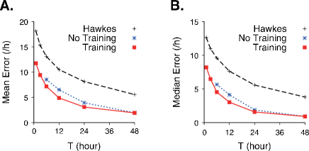
Figure 7: Dependence of the error (A: Mean, B: Median) on observation time $T$, for the three proposed models: standard Hawkes process, TiDeH without traning and TiDeH with traning. The window size $\Delta_{\rm pred}$ is set to 4 hours.

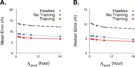
Figure 8: Dependence of the error (A: Mean, B: Median) on time resolution $\Delta_{\rm pred}$. Abbreviations of the prediction methods are the same as in Fig. 7. The observation time $T$ is fixed to 6 hours.

IV.4 Summary of TideH with training

Our selected procedure to predict future retweet activity is summarized in table 2. Given a desired value of temporal resolution $\Delta_{\rm pred}$, we proceed as follows: First, we identify the infectious rate of a tweet $p(t)$ by fitting the proposed oscillatory model. We recommend to optimize the shape parameters ($r,\phi_{0},\tau_{m}$) using a training data set, and then to estimate the intensity $p_{0}$ for the target retweet sequence. Second, we calculate the mean number of followers in the target sequence. Third, the time course of the future retweet activity $\hat{\lambda}(t)$ is evaluated by solving numerically the self-consistent equation for TiDeH (8). Finally, the retweet activity in a bin $A_{k}$ is calculated from the estimated retweet rate, $A_{k}=\int_{T+\Delta_{\rm pred}(k-1)}^{T+\Delta_{\rm pred}k}\hat{\lambda}(s)ds$. The computational cost after parameter optimization is $O(R(T)T_{\rm pred})+O(T^{2}_{\rm pred})$ where $R(T)$ is, as before, the number of observed events, and $T_{\rm pred}$ is the duration of the prediction period.

Table 2: Selected method for the prediction of future retweet activity (TiDeH with training)

1. Identify the infectious rate $p(t)$.

a) Optimize the shape parameters $(r_{0},\phi_{0},\tau_{m})$ by

minimizing the error for the training data.

b) Fit the amplitude $p_{0}$ from the retweet sequence.

2. Calculate the average number of followers.

3. Evaluate future retweet rate $\hat{\lambda}(t)$ by solving

the integral equation (8).

4. Evaluate the mean number of retweet $A_{k}$.

$A_{k}=\int_{T+(k-1)\Delta_{\rm pred}}^{T+k\Delta_{\rm pred}}\hat{\lambda}(s)ds.$

V Comparison of prediction performance with previous methods

V.1 Baseline methods for comparison

In this section, we describe four methods used as a baseline to estimate the predictive performance of our method. It should be noted that a direct comparison can not be performed because previous methods were originally designed for different prediction tasks: our work predicts the time evolution of retweet activity, whereas previous works Szabo and Huberman (2010); Zhao et al. (2015) primarily focused on predicting the final number of retweets. For this reason, we have modified three of the existing methods so that they now predict the cumulative number of retweet up to time $t$, $R(t)$. The number of retweets in the $k$-th bin $(t\in[T+(k-1)\Delta_{\rm pred},T+k\Delta_{\rm pred}])$ can then be calculated from the cumulative number of retweets by

$$A_{k}=R(T+k\Delta_{\rm pred})-R\left(T+(k-1)\Delta_{\rm pred}\right).$$

The fourth method is only used to evaluate the accuracy of TiDeH to predict the final number of retweets in the next section.

V.1.1 Linear regression (LR) Szabo and Huberman (2010).

The first method is a linear regression of the logarithm of the popularity $R(t)$ performed on a training set of $n_{\rm tr}$ tweet sequences

$$\log R(t)=\alpha_{t}+\log R(T)+\sigma_{t}\xi_{t}.$$

$\alpha_{t}$ is obtained by minimizing the squared error

$$E_{t}(\alpha_{t})=\sum_{k=1}^{n_{\rm tr}}\left\{\log R_{k}(t)-\alpha_{t}-\log R_{k}(T)\right\}^{2},$$

and $R_{k}(t)$ is the cumulative number of retweets for the $k$-th tweet in the training data and $\xi_{t}$ is a gaussian random variable with zero mean and unit variance. The variance $\sigma_{t}$ is determined by the maximum likelihood estimator $\hat{\sigma}_{t}^{2}=E_{t}(\hat{\alpha}_{t})/n_{\rm tr}$, where $\hat{\alpha}_{t}$ and $\hat{\sigma}_{t}^{2}$ are the fitted values of $\alpha_{t}$ and $\sigma_{t}^{2}$ respectively. The cumulative number of retweets $R(t)$ is predicted by the unbiased estimator

$$\hat{R}(t)=R(T)\exp(\hat{\alpha}_{t}+\hat{\sigma}^{2}_{t}/2).$$

V.1.2 Linear regression with degree (LR-N) Zhao et al. (2015).

The second method is an extension of the linear regression that incorporates the effect of the number of followers on popularity

$$\log R(t)=\alpha_{t}+\beta^{1}_{t}\log R(T)+\beta^{2}_{t}\log D(T)$$

$$+\beta^{3}_{t}\log d_{0}+\sigma_{t}\xi_{t},$$

where $D(T)=\sum_{i:t_{i}<T}d_{i}$ is the cumulative number of followers up to time $T$, $d_{0}$ is the number of followers for the original poster, and the parameters $\alpha_{t}$ and $\beta^{1,2,3}_{t}$ are obtained by minimizing the squared error

$$E_{t}(\alpha_{t},\beta^{1}_{t},\beta^{2}_{t},\beta^{3}_{t})=\sum_{k=1}^{n_{\rm tr}}(\log R_{k}(t)-\alpha_{t}$$

$$\quad-\beta^{1}_{t}\log R_{k}(T)-\beta^{2}_{t}\log D_{k}(T)-\beta^{3}_{t}\log d_{0,k})^{2}.$$

The variance $\sigma_{t}$ is then determined by the maximum likelihood estimator $\hat{\sigma}_{t}^{2}=E_{t}(\hat{\alpha}_{t},\hat{\beta}^{1}_{t},\hat{\beta}^{2}_{t},\hat{\beta}^{3}_{t})/n_{\rm tr}$, where $\hat{\alpha}_{t}$, $\hat{\beta}^{1,2,3}_{t}$, and $\hat{\sigma}_{t}^{2}$ are the fitted values of $\alpha_{t}$, $\beta^{1,2,3}_{t}$, and $\sigma_{t}^{2}$, respectively. The cumulative number of retweet $R(t)$ is predicted by the unbiased estimator

$$\hat{R}(t)=R(T)^{\hat{\beta}^{1}_{t}}D(T)^{\hat{\beta}^{2}_{t}}d_{0}^{\hat{\beta}^{3}_{t}}\exp(\hat{\alpha}_{t}+\hat{\sigma}^{2}_{t}/2).$$

V.1.3 Reinforced Poisson process (RPP) Shen et al. (2014); Gao et al. (2015).

For the third model, we adapted a recent method, which is based on a time-dependent Poisson process, where the retweet rate $\lambda(t)$ is defined as

$$\lambda(t)=cf_{\gamma}(t)r_{\alpha}(R),$$

where $f_{\gamma}(t)=t^{-\gamma}$ describes the aging effect, $r_{\alpha}(R)=\epsilon+\frac{1-e^{-\alpha(R+1)}}{1-e^{-\alpha}}$ is a reinforcement mechanism associated to the multiplicative nature of the spreading, and $R$ is the cumulative number of retweets at time $t$. The model parameters $\{c,\gamma,\alpha\}$ are determined by maximizing the likelihood function Gao et al. (2015). The log-likelihood function is maximized by the gradient descent method, and the iteration terminated when a convergence criterion is satisfied, i.e., the relative change in the parameters is lower than $10^{-4}$. The learning rate for the gradient method is set to $10^{-5}$ and the parameters are optimized in the range suggested in Gao et al. (2015), that is $1.5\leq\gamma\leq 3.5$ and $0.001\leq\alpha\leq 0.1$.

After fitting the parameters, the cumulative number of retweets is evaluated from the expectation of the Poisson process,

$$\frac{dR}{dt}=\lambda(t),$$

which can be solved exactly

$$R(t)=(\log(1+e^{x})-x-\log\tilde{\epsilon}-\alpha)/\alpha,$$

with

$$x(t)=\frac{\tilde{\epsilon}c\alpha(T^{1-\gamma}-t^{1-\gamma})}{(1-\gamma)(1-e^{-\alpha})}-(R(T)+1)\alpha$$

$$-\log(\tilde{\epsilon}-e^{-\alpha(R(T)+1)}),$$

and $\tilde{\epsilon}=1+\epsilon(1-e^{-\alpha})$. This expression is then used to predict the cumulative number of retweets.

V.1.4 SEISMIC Zhao et al. (2015).

This fourth method has recently been proposed for predicting the final number of retweets Zhao et al. (2015)

$$\hat{R}(\infty)=R(T)+\alpha_{T}\frac{\hat{p}(T)\Delta D(T)}{1-\beta_{T}\hat{p}(T)},$$

where $\hat{p}(T)$ is the infectious rate at the end of observation window $T$ and $\Delta D(T)=\sum_{i:t_{i}<T}d_{i}(1-\Phi(T-t_{i}))$. The infectious rate $\hat{p}(T)$ is estimated by a kernel estimator, and their hyper-parameters are $\alpha_{T}=0.326$, $\beta_{T}=20$ Zhao et al. (2015). Note that while the information diffusion model behind SEISMIC is a Hawkes process related to the one of TiDeH, its predictor is based on a Galton-Watson type branching process, whose parameters are fitted by the Hawkes process. In contrast, TiDeH also uses Hawkes process for the prediction of the future retweet activity. As it is designed, SEISMIC can only be applied to predict the final number of retweets, not for the future time course of retweet activity.

V.2 Prediction results

We now compare the prediction accuracy of the proposed method (TiDeH) with that of the three methods LR, LR-N and RPP. A comparison with SEISMIC is also performed when possible.

First, we have examined the dependency of the prediction performance on the observation time $T$. To do so, we have performed a 5-fold cross validation test, except for RPP as it does not require training for the prediction. As shown in Figure 9, TiDeH performs best in all the regimes, from short (1 hour) to long (48 hours) observation times, followed in order of accuracy by RPP, LR-N, and LR. In general, methods based on point processes (TiDeH and RPP) perform significantly better those based on linear regressions (LR-N and LR). We also observe that the errors increase when the observation time is decreased, and that this increase in error is minimal for TiDeH. Figure 10 is a magnified view of Figure 9 clearly showing that TiDeH outperforms RPP, with a systematic improvement of accuracy of around 20 %. On average, the error of TiDeH is 17.9 % (mean error) and 21.7 % (median error) smaller than that of RPP. Let us also note that LR-N performs much better than LR for short observation times, confirming that network information, here the number of followers, is a key ingredient for prediction improvement.

As a second step, let us consider the impact of the window size $\Delta_{\rm pred}$ on prediction performance. Figure 11 shows a similar pattern as above, with TiDeH the best predictor over all time scales, from precise (1 hour) to coarse (1 day) predictions, followed by RPP, LR-N, and LR. In general, the dependency of the error on the window size is weak, and the error slightly decreases when the window size is increased, possibly because the observation time is not sufficient to learn the retweets dynamics with a greater accuracy and/or the retweet dynamics has characteristic times larger than 1 day.

Finally, we estimate the prediction performance of TiDeH for a standard objective function, the final number of retweets. In addition to the three baseline method, we also compare its performance with the fourth baseline, SEISMIC. Figure 12 shows that TiDeH provides again the most accurate predictions for the final number of retweets. In terms of the mean and median error, we observe an improvement of around 30 % over the two runners up (SEISMIC and RPP).

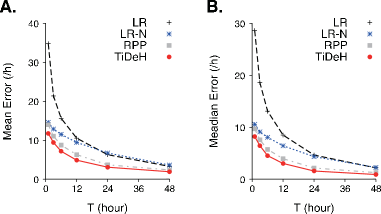
Figure 9: Comparison of prediction performance: Dependence of the error on observation time $T$. LR: Linear regression, LR-N: Linear regression with the number of followers, RPP: Reinforcement poisson process, TiDeH: proposed model. We predicted the retweet activity up to $T_{\rm max}=168$ hours from the original post with the window size $\Delta_{\rm pred}=4$ hours.

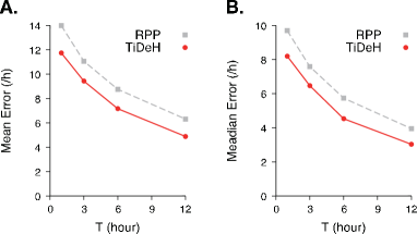
Figure 10: Magnified view of Fig. 9. Prediction performance of the best two methods (RPP and TiDeH) were shown.

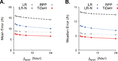
Figure 11: Comparison of prediction performance: Dependence of the error on time resolution $\Delta_{\rm pred}$. The abbreviations of the methods are the same as Fig. 9. The observation time $T$ is fixed to 6 hours.

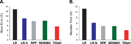
Figure 12: Comparison of prediction performance for the final number of retweets ($T=6$ hours, $T_{\rm max}=168$ hours). The abbreviations of the methods are the same as Fig. 9.

VI Conclusion and Future work

In this work, we have introduced TiDeH, a framework based on self-exciting point processes to predict the future time evolution of the popularity of a tweet. The method is based on the calibration of a model for information diffusion in social networks, which incorporates network information, circadian rhythms of online activity and aging of information. By doing so, the model provides a description based on absolute times, that is the time of the day, and relative time, that is the time since the previous triggering event, with a yet small number of parameters. As compared to previous models, our approach also has the advantage of mathematical consistency, as the modeling and the prediction tasks are performed in the same framework, and leads to a systematic improvement of accuracy in a wide range of time scales. Interestingly, our model also outperforms state-of-the-art methods to estimate the final number of retweets of a tweet, which emphasizes the importance of an appropriate modeling to solve prediction task.

Here, we have focused on the popular tweets that have more than 2,000 retweets, but the majority of information cascades on social networks are significantly shorter. It would be interesting to develop a parameter optimization technique for shorter data to overcome the limitation. Potential extensions of our work include a more detailed circadian activity by enriching the proposed model with higher harmonics and incorporating additional network information, such as correlations between number of followees and number of followers.

References

- Kwak et al. (2010) H. Kwak, C. Lee, H. Park, and S. Moon, in WWW’ 10 (2010) pp. 591–600.
- Dow et al. (2013) P. A. Dow, L. A. Adamic, and A. Friggeri, in ICWSM’ 13 (2013) pp. 145–154.
- Kumar et al. (2010) R. Kumar, M. Mahdian, and M. McGlohon, in KDD’ 10 (2010) pp. 553–562.
- Easley and Kleinberg (2010) D. Easley and J. Kleinberg, Networks, Crowds, and Markets (Cambridge university press, Cambridge, 2010).
- Goetz et al. (2009) M. Goetz, J. Leskovec, M. Mcglohon, and C. Faloutsos, in ICWSM’ 09 (2009) pp. 26–33.
- Centola (2010) D. Centola, Science 1329, 1194 (2010).
- Adar and Adamic (2005) E. Adar and L. Adamic, in 2005 IEEE/WIC/ACM International Conference on Web Intelligence (2005) pp. 207–214.
- Gruhl et al. (2004) D. Gruhl, R. Guha, D. Liben-Nowell, and A. Tomkins, in WWW’ 04 (2004) pp. 491–501.
- Salah-Brahim et al. (2012) A. Salah-Brahim, L. Tabourier, and B. Le Grand, in ICWSM’ 12 (2012) pp. 546–554.
- Weng et al. (2014) L. Weng, F. Menczer, and Y. Ahn, in ICWSM’ 14 (2014) pp. 535–544.
- Petrovic et al. (2011) S. Petrovic, M. Osborne, and V. Lavrenko, in ICWSM’ 11 (2011) pp. 586–589.
- Hong et al. (2011) L. Hong, O. Dan, and B. Davison, in WWW’ 11 (2011) pp. 57–58.
- Bao et al. (2013) P. Bao, H.-W. Shen, J. Huang, and X.-Q. Cheng, in WWW’ 13 (2013) pp. 177–178.
- Cheng et al. (2014) J. Cheng, L. Adamic, P. A. Dow, J. M. Kleinberg, and J. Leskovec, in WWW’ 14 (2014) pp. 925–936.
- Zaman et al. (2014) T. Zaman, E. B. Fox, E. T. Bradlow, et al., The Annals of Applied Statistics 8, 1583 (2014).
- Gao et al. (2015) S. Gao, J. Ma, and Z. Chen, in WSDM’ 15 (2015) pp. 107–116.
- Zhao et al. (2015) Q. Zhao, M. A. Erdogdu, H. Y. He, A. Rajaraman, and J. Leskovec, in KDD’ 15 (2015) pp. 1513–1522.
- Hawkes (1971) A. G. Hawkes, Biometrika 58, 83 (1971).
- Newman (2010) M. Newman, Networks (Oxford University Press, Oxford, 2010).
- Rogers (2010) E. M. Rogers, Diffusion of innovations (Simon and Schuster, 2010).
- Szabo and Huberman (2010) G. Szabo and B. A. Huberman, Communications of the ACM 53, 80 (2010).
- Yang and Counts (2010) J. Yang and S. Counts, in ICWSM’ 10 (2010) pp. 355–358.
- Bandari et al. (2012) R. Bandari, S. Asur, and B. Huberman, in ICWSM’ 12 (2012) pp. 26–33.
- Yang and Zha (2013) S.-H. Yang and H. Zha, in ICML’ 13 (2013).
- Matsubara et al. (2012) Y. Matsubara, Y. Sakurai, B. A. Prakash, L. Li, and C. Faloutsos, in KDD’ 12 (2012) pp. 6–14.
- Ogata (1988) Y. Ogata, Journal of the American Statistical Association 83, 9 (1988).
- Helmstetter and Sornette (2003) A. Helmstetter and D. Sornette, Journal of Geophysical Research: Solid Earth 108, 2482 (2003).
- Bacry et al. (2015) E. Bacry, I. Mastromatteo, and J.-F. Muzy, arXiv preprint arXiv:1502.04592 (2015).
- Filimonov and Sornette (2012) V. Filimonov and D. Sornette, Physical Review E 85, 056108 (2012).
- Crane and Sornette (2008) R. Crane and D. Sornette, Proceedings of the National Academy of Sciences 105, 15649 (2008).
- Masuda et al. (2013) N. Masuda, T. Takaguchi, N. Sato, and K. Yano, in Temporal Networks, Understanding Complex Systems, edited by P. Holme and J. Saramäki (Springer Berlin Heidelberg, 2013) pp. 245–264.
- Mohler et al. (2011) G. Mohler, M. Short, P. Brantingham, F. Schoenberg, and G. Tita, Journal of the American Statistical Association 106, 100 (2011).
- Golosovsky and Solomon (2012) M. Golosovsky and S. Solomon, Physical Review Letters 109, 098701 (2012).
- Shen et al. (2014) H.-W. Shen, D. Wang, C. Song, and A.-L. Barabási, in AAAI’ 14 (2014) pp. 291–297.
- Delvenne et al. (2015) J.-C. Delvenne, R. Lambiotte, and L. E. Rocha, Nature Communications 6, 7366 (2015).
- Vázquez et al. (2006) A. Vázquez, J. G. Oliveira, Z. Dezsö, K.-I. Goh, I. Kondor, and A.-L. Barabási, Physical Review E 73, 036127 (2006).
- Koyama and Shinomoto (2005) S. Koyama and S. Shinomoto, Journal of Physics A: Mathematical and General 38, L531 (2005).
- Nelder and Mead (1965) J. A. Nelder and R. Mead, The computer journal 7, 308 (1965).
- Press et al. (1996) W. H. Press, S. A. Teukolsky, W. T. Vetterling, and B. P. Flannery, Numerical recipes in C, Vol. 2 (Cambridge university press Cambridge, 1996).